Dedicated to the Global Engineering Community · FEA Information Inc. Global News & Technical...

FEA Information Inc. Global News & Technical Information

Dedicated to the Global Engineering Community

FEA Information Inc. Global News & Industry Information Issue January 2002

2____________________________________________________________________________ Livermore Software Technology Corp. www.lstc.com

FEA Information Inc. News & Technical Information

Volume 2 Issue 1-2002, January

Editorial Board: Trent Eggleston Editor Marsha Victory Feature Editor Wayne Mindle Graphics Arthur B. Shapiro Technical Writer David Benson Technical Writer Purpose:

The purpose of our free e-mailed publication is to provide technical and industry information.

New Technical Writer:

We welcome Dr. Arthur B. Shapiro as technical writer for the news and the application websites. Additionally, Dr. Shapiro will be reviewing the AVI submissions sent to FEA Information Inc. Dr. Shapiro can be reached at: [email protected]

In This Issue: 03 A New Material Model for Low Density Foams 05 Material Modeling 15 Getting Started with LS-DYNA 20 Design Space & Solid Works Help Buck Knives 23 Virtual Prototype Analysis 25 FEA Information Inc. Participant Listing 26 Website Summary Product Showcase

Welcome Participant: DYNAmore GmbH, located in Germany: www.dynamore.de Feb. Feature: Efficient and Robust Spotweld Modeling and Simulation in Crashworthiness with LS-DYNA, Karl Schweizerhof, Werner Schmid DYNAmore GmbH, Stuttgard, Germany. Additionally Karl Schweizerhof is with the Institute of Mechanics, Univ. of Karlsruhe, Germany March Feature: Post Processing

The contents of this publication is deemed to be accurate and complete. However, FEA Information Inc. doesn’t guarantee or warrant accuracy or completeness of the material contained herein. All trademarks are the property of their respective owners. This publication is published for FEA Information Inc., © Copyright. All rights reserved. Not to be reproduced in hardcopy or electronic format.

http://www.dynamore.de/


3____________________________________________________________________________ The Japan Research Institute Ltd. www.jri.co.jp

A New Material Model for Low Density Foams © Copyright FEA Information Inc. 2002

Dr. David Benson

A new material model for low density, transversely isotropic crushable foams, has been developed at DaimlerChrysler by Hirth, Du Bois, and Weimar and implemented in LS-DYNA as a user subroutine. LSTC has converted and optimized their subroutine as a new material model in LS-DYNA, and it is now generally available. Hirth, Du Bois, and Weimar determined that MAT_HONEYCOMB, which is commonly used to model foams, can systematically over estimate the stress when it is loaded off-axis. Their new material model overcomes this problem without requiring any additional input. Their new model can possibly replace the MAT_HONEYCOMB material, which is currently used in the frontal offset and side impact barriers.

Many polymers used for energy absorption are low density, crushable foams with no noticeable Poisson effect. Frequently manufactured by extrusion, they are transversely isotropic. This class of material is used to enhance automotive safety in low velocity (bumper impact) and medium velocity (interior head impact) applications. These materials require a transversely isotropic, elastoplastic material with a flow rule allowing for large permanent volumetric deformations.

The MAT_HONEYCOMB model uses a local coordinate system defined by the user. One of the axes of the local system coincides with the extrusion direction of the honeycomb in the undeformed configuration. As an element deforms, its local coordinate system rotates with its mean rigid body motion. Each of the six stress components is treated independently, and each has its own law relating its flow stress to its plastic strain.

The effect of off-axis loading on the MAT_HONEYCOMB model can be estimated by restricting our considerations to plane strain in two dimensions. Our discussion is restricted to the response of the foam before it becomes fully compacted. After compaction, its response is modeled with conventional 2J plasticity. The model reduces to

)(

)(

)(

1212

2222

1111

Vy

Vy

Vy

εσσ

εσσ

εσσ

≤

≤

≤

where Vε is the volumetric strain. For a fixed value of volumetric strain, the individual stress components respond in an elastic-perfectly plastic manner, i.e., the foam doesn’t have any strain hardening. In two dimensions, the stress tensor transforms according to

[ ] [ ] [ ][ ]

[ ]

−=

=

)cos()sin()sin()cos(

)(

)()(

θθθθ

θ

θσθσ θ

R

RR T

where θ is the angle of the local coordinate system relative to the global system. For uniaxial loading along the global 1-axis, the stress will be (accounting for the sign of the volume strain), )sgn()cos()sin(2)][sin()][cos( 1222

211

211 V

yyy εσθθσθσθσ ⋅++= assuming the strain is large enough to cause yielding in both directions.


4__________________Livermore Software T

If the shear strength is neglected, 11σ will vary smoothly between y11σ and y

22σ and never exceed the maximum of the two yield stresses. This behavior is intuitively what we would like to see. However, if the value of shear yield stress isn’t zero, 11σ will be greater than either y

11σ or y22σ . To

illustrate, if y11σ and y

22σ are equal (a nominally isotropic response) the magnitude of the stress is yy

121111 )cos()sin(2 σθθσσ ⋅+= and achieves a maximum value at 45 degrees of

yy121111 σσσ += .

For cases where there is anisotropy, the maximum occurs at a different angle and will have a different magnitude, but it will exceed the maximum uniaxial yield stress. In fact, a simple calculation using Mohr’s circle shows that the maximum value will be

( ) ( ) yyyyyy12

222112

122112

1max 4σσσσσσ +−++= .

To correct for the systematic overestimation of the off-axis strength by MAT_ HONEYCOMB, MAT_TRANSVERSELY_ISOTROPIC_CRUSHABLE_FOAM has been implemented in LS-DYNA for release in version 970 and the most recent updates of version 960. It uses a single yield surface, calculated dynamically from the six yield stresses specified by the user. The yield surface hardens and softens as a function of the volumetric strain through the yield stress functions. While the cost of the model is higher than for MAT_HONEYCOMB, its superior response off-axis makes it the model of choice for critical applications involving many types of low density foams.

Dedicated to the Engineering Community

__________________________________________________________ echnology Corp. www.lstc.com



Modeling Rigid Bodies In LS-DYNA, © Copyright Suri Bala, 2002

Livermore Software Technology Corporation

Introduction

Multi-body dynamics, i.e., the treatment of rigid bodies, in LS-DYNA is a mature capability that is used in nearly all applications. Rigid bodies are used in explicit transient calculations to represent stiff structural components that are assumed to undergo very small deformations but large translations and rotations. In crash analysis, rigid bodies are commonly used to model spot welds and engine blocks, and in manufacturing applications to model rigid tooling. Another important application is roll over simulations, where the vehicle moves freely for a significant time period without contact. During this free movement a rigid body treatment is sufficiently accurate in updating the geometry while reducing CPU time by more than order-of-magnitude. In NVH applications, the chassis can be represented by a rigid body coupled to the modal solution combined with the attachment, constraint, or inertial relief modes: this modeling technique provides a huge cost savings over explicit time integration of the degrees-of-freedom in the chassis, while providing sufficient accuracy. The rigid body treatment can also be used to impose complicated boundary conditions involving subsets of nodal points.

Defining Rigid Bodies

There are a number of ways to define rigid bodies in LS-DYNA. However, the most straightforward method is to define an accurate finite element mesh for the part and when assigning constitutive properties on the *PART card, simply use a *MAT_RIGID constitutive model. In the *MAT_RIGID definition, the mass density and elastic constants of the rigid material are given. Later, if it turns out that experimental test show significant deformations in the rigid part, the *MAT_RIGID definition can be trivially replaced by an elastic-plastic constitutive model with the same elastic constants and no other input changes will be necessary. Another advantage of an accurate finite element mesh, besides the obvious one of visualization, is that the inertia tensor, the total rigid mass, and the mass center are automatically calculated using the input mass density and do not need to be separately defined. Also, parts contacting the rigid body will transmit forces at the proper geometric locations, which would not be possible if a crude geometric representation is used for the rigid body. The contact stiffness for penalty based contact is computed from the elastic constants defined in the *MAT_RIGID input so realistic values are always recommended. In the *SECTION definition all element formulations for the different element types, i.e., beams, shells, etc., can be used for rigid bodies. Since no numerical integration is performed at the element level if the element is rigid, the number of integration points specified here is irrelevant. No storage is allocated for the integration points in the rigid materials, unless the material starts as deformable with the intent that it will be switched to rigid later in the calculation, for example, in roll over.



Frequently, the use of an accurate mesh for the rigid body is unnecessary, since the surface geometry is of interest: not the solid material beneath the surface. This is true in modeling the tooling used in manufacturing and the engine blocks used in crash modeling. In the latter case, unlike the former where all motion is prescribed, the center-of-mass, the total mass, and inertia tensor must be accurate. The *PART_INERTIA definition is used to define these quantities directly.

Rigid bodies can be defined without elements by providing a list of nodal points that are included in the rigid body definition. This is done through the following three options: *CONSTRAINED_NODAL_RIGID_BODY, *CONSTRAINED_SPOTWELD, and *CON-STRAINED_GENERALIZED_WELD. If necessary, the INERTIA option can be used with the nodal rigid body definition. The disadvantage of the nodal rigid body is that no surface exist for contact, assuming that null shells are not used, and that visualization during post-processing is difficult. However, the nodes in the nodal rigid body can be treated in the node to surface contact definitions. Rigid bodies can share nodes with deformable bodies. The mass of the shared nodes, which belongs to the deformable body, is added to the rigid body’s mass and inertia tensor. If the INERTIA option is used to define the rigid body mass and inertia tensor, then it is the responsibility of the user to include the shared mass of merged nodal points. The ability to couple rigid bodies to deformable bodies by shared nodes makes it very easy to add deformable materials to rigid body dummy models to obtain more realistic responses. To attach deformable materials to rigid bodies when the nodes are not shared is quite simple. Tied contact interfaces based on constraint equations cannot be used; rather, the interface nodes in the deformable material that should move with the rigid body should be slaved to the rigid body by the keyword, *CONSTRAINED_EXTRA_NODES, as discussed below.

Constraints on Rigid Bodies

Constraints on rigid bodies can be applied in either the global or local coordinate systems. The parameters CON1 and CON2 in the *MAT_RIGID definition are used to define the appropriate constraints on the rigid body. However, during the rigid body initialization, LS-DYNA checks all nodal constraints in the set of rigid body nodes and determines whether any of the six degrees-of-freedom of the rigid body are globally constrained: if so, CON1 and CON2 are set automatically, and this information is written into the D3HSP file. If a global constraint cannot be determined from the constraints on the rigid body nodes, a penalty method is used to impose the constraints directly on the nodes. This latter method is not always reliable due to the difficulty of determining an optimal value for the penalty. To properly tie a rigid body at a node the use of a joint with the Lagrange multiplier option is preferred since it eliminates the uncertainties of the penalty formulation. Constraints on the rigid body that apply in the local coordinate system are specified by setting the input parameter CMO to -1, CON1 to the ID of the local coordinate system, and CON2 to the desired constraint value. For example, setting CON2 to “111111” would fix all



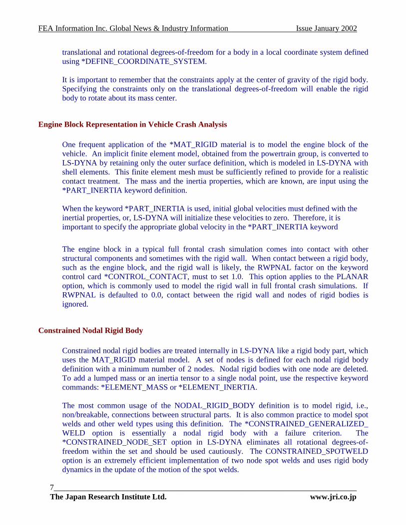
translational and rotational degrees-of-freedom for a body in a local coordinate system defined using *DEFINE_COORDINATE_SYSTEM. It is important to remember that the constraints apply at the center of gravity of the rigid body. Specifying the constraints only on the translational degrees-of-freedom will enable the rigid body to rotate about its mass center.

Engine Block Representation in Vehicle Crash Analysis

One frequent application of the *MAT_RIGID material is to model the engine block of the vehicle. An implicit finite element model, obtained from the powertrain group, is converted to LS-DYNA by retaining only the outer surface definition, which is modeled in LS-DYNA with shell elements. This finite element mesh must be sufficiently refined to provide for a realistic contact treatment. The mass and the inertia properties, which are known, are input using the *PART_INERTIA keyword definition.

When the keyword *PART_INERTIA is used, initial global velocities must defined with the inertial properties, or, LS-DYNA will initialize these velocities to zero. Therefore, it is important to specify the appropriate global velocity in the *PART_INERTIA keyword

The engine block in a typical full frontal crash simulation comes into contact with other structural components and sometimes with the rigid wall. When contact between a rigid body, such as the engine block, and the rigid wall is likely, the RWPNAL factor on the keyword control card *CONTROL_CONTACT, must to set 1.0. This option applies to the PLANAR option, which is commonly used to model the rigid wall in full frontal crash simulations. If RWPNAL is defaulted to 0.0, contact between the rigid wall and nodes of rigid bodies is ignored.

Constrained Nodal Rigid Body

Constrained nodal rigid bodies are treated internally in LS-DYNA like a rigid body part, which uses the MAT_RIGID material model. A set of nodes is defined for each nodal rigid body definition with a minimum number of 2 nodes. Nodal rigid bodies with one node are deleted. To add a lumped mass or an inertia tensor to a single nodal point, use the respective keyword commands: *ELEMENT_MASS or *ELEMENT_INERTIA. The most common usage of the NODAL_RIGID_BODY definition is to model rigid, i.e., non/breakable, connections between structural parts. It is also common practice to model spot welds and other weld types using this definition. The *CONSTRAINED_GENERALIZED_ WELD option is essentially a nodal rigid body with a failure criterion. The *CONSTRAINED_NODE_SET option in LS-DYNA eliminates all rotational degrees-of-freedom within the set and should be used cautiously. The CONSTRAINED_SPOTWELD option is an extremely efficient implementation of two node spot welds and uses rigid body dynamics in the update of the motion of the spot welds.



Merging Rigid Bodies

Components, such as an engine block, are made of an assembly of discrete parts. One way to model an entire assembly as a rigid body is to simply put all elements in the assembly of parts into one *PART keyword and assign a *MAT_RIGID material type. This works if all elements are of the same type since under the *PART definition the *SECTION ID defines the element type for the entire part. In general though, within an assembly of parts, many different element types are needed. So as an alternative, the keyword *CONSTRAINED_ RIGID_BODIES can be used to define a single rigid body that contains many different element types. The input, as shown in Figure 1.1, requires a master part ID and a slave part ID. LS-DYNA internally merges the two bodies and treat them as one. An unlimited number of slave parts can be merged to a given master part. This feature enables the user to keep the individual parts of the assembly as separate components in the pre-processor and post-processor but treat them as one internally. Plus it allows a given rigid body to be made up of all available element types.

Figure 1.1 Merging Rigid Bodies using *CONSTRAINED_RIGID_BODIES

Defining Structural Connections to A Rigid Body

To rigidly constrain an arbitrary nodal point of a deformable body to a rigid body, which is defined as a *MAT_RIGID material, use the *CONSTRAINED_EXTRA_NODE_ keyword. The required input parameters are the master part ID and the node set ID. The node set includes the nodes that are rigidly attached to the master part ID, and these nodes can be physically located anywhere in the model, i.e., they do not need to be adjacent to a rigid surface. Consequently, it is possible to add deformable materials to a rigid component of a dummy without an accurate mesh for the rigid component.

Slave Part IdMaster Part Id



Rigid Body Output

All relevant rigid body time history data is output to the ASCII file, RBDOUT (Rigid Body Data Output). The data can be output in both global and local coordinate systems. In the latter case the local system, defined in the *MAT_RIGID input, is updated each cycle to track the orientation of the rigid body. It is generally recommended to request this output for each analysis. In some cases, the file size could be very large, as it contains, by default the output for every *CONSTRAINED_NODAL_RIGID_BODY as well. Such output can be controlled in the input file.

Deformable to Rigid Material Switching

Occasionally, long duration, large rigid body motions arise that are prohibitively expensive to simulate if the elements in the model are deformable. Such a case occurs in automotive rollover where the time duration of the rollover dominates the cost relative to the post impact response that occurs much later. To permit such simulations to be efficiently handled a capability to switch a subset of materials from deformable to rigid and back to deformable is available. Such switching is done with the *DEFORMABLE_TO_RIGID keyword input. In practice, the suspension system and tires would remain deformable. If this option is active, LS-DYNA knows that all materials in the model have the potential to become rigid bodies sometime during the calculation. When this flag is set, a cost penalty is incurred on vector processors since the blocking of materials in the element loops will be based on the part ID rather than the material type ID. Normally this cost is insignificant relative to the cost reduction due to this unique feature. For rigid body switching to work properly, the choice of the shell element formulation is critical. The Hughes-Liu elements cannot be used for two reasons. Since these elements compute the strains from the rotations of the nodal fiber vectors from one cycle to the next, the nodal fiber vectors should be updated with the rigid body motions, and this is not done. Secondly, the stresses are stored in the global system as opposed to the co-rotational system.

Slave Node Set Id

Master Part



Therefore, the stresses would also need to be transformed with the rigid body motions or zeroed out. The co-rotational elements of Belytschko and co-workers do not reference nodal fibers for the strain computations, and the stresses are stored in the co-rotational coordinate system which eliminates the need for the transformations; consequently, these elements can be safely used. The membrane elements and airbag elements are closely related to the Belytschko shells and can be safely used with the switching options. The beam elements have nodal triads that are used to track the nodal rotations and calculate the deformation displacements from one cycle to the next. These nodal triads are updated every cycle with the rigid body rotations to prevent non-physical behavior when the rigid body is switched back to deformable. This applies to all beam element formulations in LS-DYNA. The Belytschko beam formulations are preferred for the switching options for like the shell elements, the Hughes-Liu beams keep the stresses in the global system . Truss elements, like the membrane elements, pose no difficulties. The brick elements store the stresses in the global system and upon switching the rigid material to deformable the element stresses are zeroed to eliminate spurious behavior. The implementation for switching addresses many potential problems and has worked well in practice. The current restrictions can be eliminated if the need arises and should pose no insurmountable problems. We will continue to improve this capability if we find that it is becoming a popular option.

Rigid Body Welds

The weld capability in LS-DYNA is based on rigid body dynamics. Each weld is defined by a set of nodal points which moves rigidly with six degrees of freedom until a failure criteria is satisfied. Five weld options are implemented including: • Spot weld. • Fillet weld • Butt weld • Cross fillet weld • General weld Welds can fail three ways: by ductile failure which is based on the effective plastic strain, by brittle failure which is based on the force resultants acting on the rigid body weld, and by a failure time, which is specified in the input. When effective plastic strain is used, the weld fails when the nodal plastic strain exceeds the input value. A least squares algorithm is used to generate the nodal values of plastic strains at the nodes from the element integration point values. The plastic strain is integrated through the element and the average value is projected to the nodes with a least square fit. In the resultant based brittle failure, the resultant forces and moments on each node of the weld are computed. These resultants are checked against a failure criterion which is expressed in terms of these resultants. The forces may be averaged over a user specified number of time steps to eliminate breakage due to spurious noise. After all nodes of a weld are released the rigid body is removed from the calculation.



Rigid Body Joints

Joints are used to join rigid bodies. A major application of joints in crashworthiness analysis is in modeling dummies. Whether a dummy is rigid or deformable, the “skeleton” is usually constructed of rigid bodies tied together by joints. The joints eliminate one or more degrees-of-freedom. For example, a spherical joint eliminates three translational degrees-of-freedom when placed between two rigid bodies leaving three translational and six rotational degrees-of-freedom. The joints are implemented using two methods in LS-DYNA: penalties and Lagrange multipliers. The penalty method is the default method. The Lagrange multiplier method can be activated for all rigid bodies on the *CONTROL_RIGID keyword or, if desired, for a subset of rigid bodies in the input for the Joint definitions. The Lagrange multiplier approach requires an iterative solution with the assembly and inversion of the rigid body inertia matrix each cycle and, consequently, it is slightly more expensive. Here we will briefly describe the penalty approach. Given a constraint equation ( ), 0i jC x x = , for nodes i and j , the penalty function added to the

Lagrangian of the system is ( )21/ 2 ,i jkC x x− . The resulting nodal forces are:

( ) ( ),, i j

i i ji

C x xf kC x x

x∂

∂= −

( ) ( ),, i j

j i jj

C x xf kC x x

x∂

∂= −

The forces acting at the nodes are converted into forces and moments acting on the rigid body The joint constraints are defined in terms of the displacements of individual nodes. Regardless of whether the node belongs to a solid element or a structural element, only its translational degrees of freedom are used in the constraint equations. A spherical joint is defined for nodes i and j by the three constraint equations: 1 1 2 2 3 30 0 0i j i j i jx x x x x x− = − = − = and a revolute joint, which requires five constraints, is defined by two spherical joints, for a total of six constraint equations. Since a penalty formulation is used, the redundancy in the joint constraint equations is unimportant. A cylindrical joint is defined by taking a revolute joint and eliminating the penalty forces along the direction defined by the two spherical joints. In a similar manner, a planar joint is defined by eliminating the penalty forces that are perpendicular to the two spherical joints. The magnitude of the penalty stiffness k is chosen automatically so that it does not control the stable time step size for the explicit solution. For the central difference method, the stable time step t∆ is restricted by the condition that,



2t∆ =Ω

where Ω is the highest frequency in the system. The six vibrational frequencies associated with each rigid body are determined by solving their eigenvalue problems assuming 1k = . For a body with m constraint equations, the linearized equations of the translational degrees of freedom are 0MX mkX+ = and the frequency is /mk M where M is the mass of the rigid body. The corresponding rotational equations are 0J Kθ θ+ = J is the inertia tensor and K is the stiffness matrix for the moment contributions from the penalty constraints. The stiffness matrix is derived by noting that the moment contribution of a constraint may be approximated by ( )x

i iF kr rθ= − × ×

cmi ir x X= −

and noting the identity,

( )A B C A C A C B× × = ⋅ − ⊗ so that

[ ]1

m

i i i ii

K k r r r r=

= ⋅ − ⊗

The rotational frequencies are the roots of the equation 2det 0K J− Ω = , which is cubic in 2Ω .

Defining the maximum frequency over all rigid bodies for k=1 as maxΩ , and introducing a time step scale factor TSSF , the equation for k is

2

max

2TSSFkt

≤ ∆ Ω

Generally, the stiffness determined in this way is quit stable; however, there always exist problems where the computed stiffness is too large or small. In these cases, a scale factor can be defined.



Built-in Rigid Body Dummies

Rigid body dummies are generated and simulated within LS-DYNA by including the appropriate *COMPONENT keyword; both the GEBOD and Hybrid III variety of dummy can be created. Accordingly the term “built-in” is used to refer to the *COMPONENT dummies for their meshes are automatically generated when the simulation is initialized. Moreover, the motion of the dummy, represented by a multi-body system of rigid segments, is governed by differential equations. These motion equations are integrated within LS-DYNA separately from the finite element model. Interaction between the finite element structure and dummy is achieved through conventional contact interfaces.

Using the keyword *COMPONENT_GEBOD either a male, female or child humanoid can be brought into the finite element model. Physical properties of these dummies draw upon the GEnerator of BODy database representing an extensive human measurement program conducted by government agencies. Size of the male and female subjects is specified as a combined height and weight percentile ranging from 0 to 100. The age of the genderless child, ranging from 24 to 240 months, is used to specify its size. Twenty-two ellipsoids comprise the GEBOD dummy and gives rise to a dynamical system possessing forty degrees of freedom. Connecting the rigid segments are joints whose properties (stiffness, damping, stop angles, etc.) are set to default values but may altered with the keyword *COMPONENT_GEBOD_JOINT. Although conventional contact interfaces (e.g., *CONTACT_SURFACE_TO_SURFACE) work well, non-faceted contact interfaces can be applied with *CONTACT_GEBOD.

A family of 5th, 50th, and 95th percentile Hybrid III dummies is available with the keyword *COMPONENT_HYBRIDIII. The detailed mesh generated by this command closely matches the topology of the industry standard Hybrid III crash test dummy. Forty-two variables suffice to describe the motion of the nineteen segments comprising this system. Although the underlying segments of the dummy are rigid it is possible to optionally specify deformable materials for the jacket, pelvis, and head skin. The user may change the default joint properties with *COMPONENT_HYBRIDIII_JOINT. Including the keyword *DATABASE_H3OUT causes joint forces and torques to be written to an ASCII output file.

Future

In version 960 of LS-DYNA the use of rigid bodies in implicit calculations is limited since key capabilities such as joint constraints are not implemented. In version 970, nearly all explicit rigid body capabilities are available including dynamics and the complete set of joints. These options are available for implicit linear and nonlinear solutions. Eigenvalue extraction is now possible in version 970 with virtually all constraint options, including rigid bodies with joint connections.



Getting Started with LS-DYNA © Copyright FEA Information Inc. 2002

Following are the first 3 chapters of the “Getting Started with LS-DYNA” user manual. As chapters are completed, they will be included in subsequent newsletters. The entire “Getting Started with LS-DYNA” manual, completed to date, will be available for downloading from the www.feainformation.com website under the link Tutorials starting February 2, 2002.

1 Introduction LS-DYNA is used to solve multi-physics problems including solid mechanics, heat transfer, and fluid dynamics either as separate phenomena or as coupled physics, e.g., thermal stress or fluid structure interaction. This manual presents “very simple” examples to be used as templates (or recipes). This manual should be used side-by-side with the “LS-DYNA Keyword User’s Manual”. The keyword input provides a flexible and logically organized database. Similar functions are grouped together under the same keyword. For example, under the keyword, *ELEMENT, are included solid, beam, and shell elements. The keywords can be entered in an arbitrary order in the input file. However, for clarity in this manual, we will conform to the following general block structure and enter the appropriate keywords in each block.

1. define solution control and output parameters 2. define model geometry and material parameters 3. define boundary conditions

2 Units LS-DYNA requires a consistent set of units to be used. All parameters in this manual are in SI units. General

• length [m] • mass [kg] • temperature [K] • time [sec]

Mechanical units • density [kg/m3] • Modulus of elasticity [Pa] • yield stress [Pa] • coefficient of expansion [m/m K]

Thermal units • heat capacity [J/kg K] • thermal conductivity [W/m K] • heat generation rate [W/ m3]

http://www.feainformation.com/


15_________________________________The Japan Research Institute Ltd.

3 Getting Started

3.1 Problem Definition Consider the deformation of an aluminum block sitting on the floor with a pressure applied to the top surface.

3.2 Input File Preparation The first step is to create a mesh and define node points. Since we are just getting started, we will define the mesh as consisting of only 1 element and 8 node points as shown in the following figure. Also, we will use default values for many of the parameters in the input file, and therefore not have to enter them. 5 8 6 7 1 4 2 3 The following steps are required to create the

The first line of the input file mcontaining the “keyword” formDYNA releases.

1m

P = 70.e+05 Pa Aluminum 1100-O density 2700 kg/m3 modulus of elasticity 70.e+09 Pa Poisson Ratio 0.3 coefficient of expansion 23.6e-06 m/m K heat capacity 900 J/kg K thermal conductivity 220 W/m K

*KEYWORD

The “LS-DYNA Keyword User’s Manual” should be read side-by-side with this manual.

___________________________________________ www.jri.co.jp

finite element model input file.

ust begin with *KEYWORD. This identifies the file as at instead of the “structured” format of older LS-



The first input block is used to define solution control and output parameters. As a minimum, the *CONTROL_TERMINATION keyword must be used to specify the problem termination time. We will apply the pressure load as a ramp from 0 Pa to 70.e+05 Pa during a time interval of 1 second. Therefore, the termination time is 1 second. Additionally, one of the many output options should be used to control the printing interval of results (e.g., *DATABASE_BINARY_D3PLOT). We will print results every 0.1 seconds. The second input block is used to define the model geometry, mesh, and material parameters. The following description and map may help to understand the data structure in this block. We have 1 part, the aluminum block, and use the *PART keyword to begin the definition of the finite element model. The *PART keyword contains data that points to other attributes of this part, e.g., material properties. Keywords for these other attributes in turn point elsewhere to additional attribute definitions. The organization of the keyword input looks like this. The LS-DYNA Keyword User Manual should be consulted at this time for a description of the keywords used above. A brief description follows: *PART We have 1 part identified by part identification (pid=1). This part has attributes

identified by section identification (sid=1) and material identification (mid=1). *SECTION_SOLID Parts identified by (sid=1) are defined as constant stress 8 node brick elements

by this keyword. *MAT_ELASTIC Parts identified by (mid=1) are defined as elastic materials with a modulus of

elasticity E and a Poisson ratio of µ by this keyword. *ELEMENT_SOLID Eight node solid brick elements identified by element identification (eid=1)

have the attributes of (pid=1) and are defined by the node list (nid)

*CONTROL TERMINATION1.

*DATABASE_BINARY_D3PLOT.1

*PART pid sid mid

*SECTION_SOLID sid

*MAT_ELASTIC mid den E µ

*ELEMENT_SOLID eid pid nid1 nid2 ..

*NODE nid1 x y z


*NODE The node identified by (nid) has coordinates x,y,z. Our finite element model consists of 1 element, 8 nodes, and 1 material. Keeping the above in mind, the data entry for this block looks like this.

The third input block is used to define boundary conditions and time dependent load curves. We are applying a load of 70.e+05 Pa to the top surface of the block defined

by nodes 5-6-7-8. We will ramp the load up from 0 Pa to 70.e+05 Pa during a time interval of 1 second.

Note that the first data entry in *LOAD_SEGMENT is a load curve identification number (lcid=1) which points to the load curve defined by the keyword *DEFINE_CURVE having that same (lcid) identification number.

3Tfs

*PARTaluminum block

1 1 1*SECTION_SOLID

1*MAT_ELASTIC

1 2700. 70.e+09 .3*ELEMENT_SOLID

1 1 1 2 3 4 5 6 7 8*NODE

1 0. 0. 0. 7 72 1. 0. 0. 5 03 1. 1. 0. 3 04 0. 1. 0. 6 05 0. 0. 1. 4 06 1. 0. 1. 2 07 1. 1. 1. 0 08 0. 1. 1. 1 0

*LOAD SEGMENT1 1. 0. 5 6 7 8

*DEFINE_CURVE1

0. 0.1. 70.e+05


The last line in the input file must have the keyword *END.

.3 LS-DYNA solution he vertical and horizontal displacement of node 7, calculated by LS-DYNA, are shown in the

ollowing 2 graphs. The solution to this simple problem can be calculated analytically. The LS-DYNA olution compares exactly with the analytical solution.

*END



The vertical displacement due to a 70.0e+05 Pa pressure load can be calculated by

( )( )( ) =

++==∆

097010570

ee

EPll

0.1e-03 m

The horizontal displacement is

( )( ) ==∆=∆ 0001.03.0llh µ 0.03e-03 m



Engineers at Buck Knives, Inc., the world's leading manufacturer of sporting knives and tools for outdoor activities, recently faced the seemingly insurmountable challenge of designing and producing a new version of the company's BuckTool™-a compact, multi-function, folding tool-in record time. The pressure was on Buck Knives' product development staff to slash the existing design/production cycle of more than one year, so the company could introduce the product to the mass-merchant market (outlets such as Wal-Mart, Kmart, etc.) in time to capitalize on the holiday buying season. Buck Knives, based in El Cajon, California, undertook the BuckLite(tm) Tool project as part of a strategic business initiative to expand beyond the company's traditional retail space of hardware stores, hunting/fishing shops, catalogs, and sporting goods outlets, into the mass-merchant space, sometimes referred to as the "marts." Introducing the new product quickly to this market was more than an engineering challenge; it was a major business opportunity and objective. Tom Gaboury, engineering designer at Buck Knives, said the BuckLite Tool, which includes a set of needle-nose pliers, a Phillips screwdriver bit, three slotted screwdriver bits, a file, an awl, a bottle opener, a wire cutter, and a knife blade, will be introduced in August 1997. The timing of the product release, in advance of the holiday buying season, has already resulted in pre-production sales of over 100,000 units and a major accomplishment for Buck Knives in securing its place in a new market.

DesignSpace Speeds Time to Market

According to Gaboury, the major factor in meeting the BuckLite Tool challenge was the acquisition and use of SolidWorks 97 and DesignSpace for SolidWorks. Implementing these software packages to drive the project helped Buck Knives produce the following results: The design/production cycle for the BuckLite Tool was cut to six months, a reduction of more than 50 percent from the company's traditional design cycle.

Design costs were dramatically reduced. Each design/prototype iteration costs Buck Knives roughly $2,000 to develop new molds and castings. Historically, several design iterations were required. Using DesignSpace for SolidWorks, engineers created a high-quality design the first time. Product performance was improved almost three-fold. The pliers on the original BuckTool design could sustain a force of 1,000 pounds before failure (that product has been redesigned and presently can sustain a

DesignSpace and SolidWorks Help Buck Knives Capture Major New Market Opportunity © Copyright ANSYS Inc.

Reprinted from the ANSYS Inc. Website www.ansys.com



force of up to 1,800 pounds). The pliers on the BuckLite Tool, which was designed using DesignSpace, can handle a force of up to 2,700 pounds.

"The DesignSpace Stress Wizard is so easy, I couldn't believe it," Gaboury said. "I've never had any finite element analysis (FEA) experience. DesignSpace makes it so easy. It's outstanding. It's what everyone's been looking for." Gaboury used the DesignSpace Stress Wizard as he created the design for the jaws on the needle-nose pliers that are a part of the BuckLite Tool. He ran several stress failure analyses as he designed, tweaking his model based on the results he received as he went along. All of the design work was completed on a Micron(r) computer with a 150 MHz Pentium processor and 64 MB of RAM. "I created the model, and the DesignSpace analysis ran in 10 minutes," Gaboury explained. " I ran a number of analyses, changing some radii, forces, and load directions along the way....DesignSpace helped me to nail the design the first time."

Gaboury pointed out that he was mostly concerned about the strength of the tool in the lug area, where the tool handle attaches to the jaw of the pliers, and that as a design engineer, he did not need the specialization of a traditional FEA package to obtain answers to his design questions. "All we want to know is will the part break or not," he added. "DesignSpace fits my needs, exactly."

Getting Up to Speed Quickly The most surprising part of the project, according to Gaboury, was how quickly he was able to use SolidWorks and DesignSpace for SolidWorks, both of which were purchased from Digital Dimensions, Inc., the SolidWorks and DesignSpace VAR for Southern California. Gaboury completed the proj ect after using SolidWorks for just eight weeks and after using DesignSpace for just two weeks.

Will It Break? Like many mainstream product manufacturers, Buck Knives' top priority, even more important than time to market, was product performance. Making the deadline did not supersede continuing the standard of high-quality products that Buck Knives is known for. In the past, the company would design a part, then send it on to Hitchiner Manufacturing Company, Inc., a ferrous and nonferrous investment casting firm based in Milford, N.H., for mold development and casting. The prototypes are then sent back to Buck Knives for pull and pressure testing on hydraulic-driven mechanisms equipped with strain gauges.



Without DesignSpace software, Buck Knives would have made design changes via prototype testing, which could have required numerous castings. Gaboury noted that the cost of the castings was not the primary concern for the BuckLite Tool project team. Time was of the essence. They had to be ready in time for the holiday buying season. "How much money has this one analysis saved? That's hard to say because we don't really know how many design iterations would have been required without it," Gaboury explained. "What you really lose is time. We're looking at five-to-six weeks to redesign and test each time. This software (DesignSpace) got us past that. How do you put a value on that? I don't know, but for this project, I can tell you it's big. It's real big." In addition to the time savings afforded by using DesignSpace software, additional time was saved simply by using SolidWorks 97 for solid modeling, which in and of itself eliminated three or four sets of prototypes. The combination of SolidWorks 97 and the DesignSpace Stress Wizard for SolidWorks helped Buck Knives engineers produce a higher quality product, at lower cost, and within the confines of a very tight deadline. The software not only satisfied a technical need. It met a business challenge; just in time for the holidays. April 22-24, 2002 USA

ANSYS Users Conference & Exhibition 2002 - Pittsburgh Hilton, Pittsburgh, PA. For information visit:

2002 Events/Conferences

Feb 22-23 Gisseta India Pvt. Ltd: 1st National Conference on CAD/CAE (Feb 22-23, 2002) The Conference will be held at "GRT Grand Days", Chennai, India - Hosted by GissEta, Co-hosted by LSTC and ETA

April 08-10 FRANCE

MSC.Software Worldwide Aerospace Conference & Technology Showcase, Toulouse, France

May 19-21, USA

LSTC & ETA: 7th International LS-DYNA User's Conference at the Hyatt Regency Hotel & Conference Center - Fairlane Town Center, Dearborn, MI 48126

Oct. 9-11

CAD-FEM Users Meeting - International Congress on FEM Technology: Kultur- und Congress-Centrum "Graf-Zeppelin-Haus", Friedrichshafen, Lake Constance, Germany. For information contact Barbara Leichtenstern. Information will be available soon on the CAD-FEM website

http://www.hyatt.com/usa/detroit/hotels/hotel_dttrd.html



Virtual Prototype Analysis,

© Copyright OASYS, Ltd. – The full article can be viewed on www.arup.com/dyna

(applications) Vehicles and other manufactured products have to be durable. They are commonly subjected to tests involving repeated loads and one-off extreme loads to assess their durability performance. The tests are sometimes modelled using linear finite element analysis, in which the loading is estimated from experience. This technique gives poor results, because the stiffness and strength of the structure often controls the applied force, so design changes intended to reduce deformation can instead lead to unexpected failures. In the vehicle industry, durability tests may be modelled by a multi-step analysis process involving simplifying assumptions at each stage. The errors that arise from this type of analysis process are becoming unacceptable in today’s shorter product development cycles, because there is no longer time to find and correct problems by testing. Many advantages can be obtained by simulating the tests as they are done in practice, including all the dynamic and nonlinear effects, in a single simulation. LS-DYNA is ideally suited to simulate many of these tests.

An example is the modelling of events from accelerated durability tests and suspension abuse loads on cars. The loading is determined by tyre behaviour, suspension response, and the flexibility of the suspension members, bushes, and body. By including all of these items in the calculation, a potentially more accurate simulation can be achieved. In the abuse load cases, damage to the body and suspension can be predicted.



The modelling techniques are very similar to those for crash analysis, except that the suspension and tyres are modelled more accurately. The tyres each contain around 1500 orthotropic shell elements; often, solid elements are added to represent the tread. The LS-DYNA airbag feature is used to control the internal pressure.

The analyses shown in the pictures on this page were all run using standard LS-DYNA 940 on a 64-bit Cray computer. It is recommended that a double precision version of LS-DYNA should be used for this type of calculation if the solver normally uses 32-bit word length, as is the case with most unix workstations



FEA Information Inc. Participants Headquarters Company website

Australia Leading Engineering Analysis Providers www.leapaust.com.au Belgium LMS, International www.lmsintl.com Canada Metal Forming Analysis Corp. www.mfac.com China ANSYS Bejing www.ansys.com (link on international) France Dynalis www.dynalis.fr Germany DYNAmore www.dynamore.de Germany CAD-FEM www.cadfem.de India GissEta www.gisseta.com Japan The Japan Research Institute, Ltd www.jri.co.jp Japan Fujitsu Ltd. www.fujitsu.com Korea THEME Engineering www.lsdyna.co.kr Korea Korean Simulation Technologies www.kostech.co.kr Russia State Unitary Enterprise - STRELA www.ls-dynarussia.com Sweden Engineering Research AB www.erab.se Taiwan Flotrend Corporation www.flotrend.com UK OASYS, Ltd www.arup.com /dyna USA Livermore Software Technology www.lstc.com USA Engineering Technology Associates www.eta.com USA ANSYS, Inc www.ansys.com USA Hewlett Packard www.hp.com USA SGI www.sgi.com USA MSC Software www.mscsoftware.com USA EASi Engineering www.easiusa.com USA DYNAMAX www.dynamax-inc.com

FEA Information Educational Participants Dr. T. Belytschko

Northwestern U. - USA Dr. D. Benson UCSD - USA

Dr. Bhavin V. Mehta Ohio Univ. - USA

Dr. Taylan Altan

The Ohio State U. – ERC/NSM - USA

Prof. Ala Tabiei U. of Cincinnati - USA

Dr. Alexey I. Borovkov St. Petersburg State Technical.

Univ. Russia



FEA Information News Showcased in November Archived on the site on the News Page

December 3rd

Software LSTC LS-OPT Software MSC NASTRAN Distributor THEME Located in Korea

December 10th

Software LMS Virtual .Lab Software JRI J-STAMP Distributor Dynalis Located in France

December 24th

Software: EASI Engineering EASi-Crash Application Oasys, Ltd. Heart Valve Analysis Distributor GissEta Located in India

December 31st

Year End Participant Showcase: Livermore Software Technology Corp.

FEA Information welcomes readers’ letters, articles, and papers for publication in the International News. FEA Information is particularly interested in learning how the reader is using FEA Information Inc. Participant’s software and hardware in solving their engineering problems. Submissions should be approximately 5 pages (including graphics) and as a word doc not more than 150KB (including graphics). The author of any item selected for publication will be required to release their copyright in favor of FEA Information Inc. Due to legal reasons and editorial policy, articles comparing products and services are ineligible for publication. Unless the author requests anonymity, FEA Information Inc. will be pleased to include his or her name and country of residence.

Questions should be sent to [email protected] - We will be pleased to discuss your article and/or ideas for an article.

mailto:[email protected]


News Showcase

ApEle l Rec

Fea e time dom

For

Livermore Software Technology Corporation

[www.ls-dyna.com] [www.lstc.com]

The Japan Research Institute Limited

www.jri.co.jp

plications: Antennas, Electronic Devices, PCBs, Strip Lines, EMC, Wave Absorbers, ctromagnetic Shields, Waveguides, Resonators, Plasma, Optical Pickups, Magneto-Opticaording, Cellular Phones, Microwave Ovens

tures: Analysis selectable either in the frequency domain (Finite Element Method) or thain (Finite Difference Time Domain) depending on the problem.

• Both dielectric and magnetic material properties may be frequency dependent. • Coupled thermal analysis

For More InformationAvailability

26____________________________________________Livermore Software Technology Corp.

Complete Information on JMAG-Studio: http://www.jri.co

on

________________________________ www.lstc.com

.jp/pro-eng/jmag/e/jmg/index.html

Dedicated to the Global Engineering Community · FEA Information Inc. Global News & Technical...

Documents

Transcript of Dedicated to the Global Engineering Community · FEA Information Inc. Global News & Technical...