Decorrelated Variable ImportanceIsabella Verdinelli and Larry Wasserman

November 19 2021

Because of the widespread use of black box prediction methods such as random forests and neural nets, thereis renewed interest in developing methods for quantifying variable importance as part of the broader goalof interpretable prediction. A popular approach is to define a variable importance parameter — known asLOCO (Leave Out COvariates) — based on dropping covariates from a regression model. This is essentiallya nonparametric version of R2. This parameter is very general and can be estimated nonparametrically,but it can be hard to interpret because it is affected by correlation between covariates. We propose a methodfor mitigating the effect of correlation by defining a modified version of LOCO. This new parameter isdifficult to estimate nonparametrically, but we show how to estimate it using semiparametric models.

1. Introduction

Due to the increasing popularity of black box prediction methods like random forests and neu-ral nets, there has been renewed interest in the problem of quantifying variable importance inregression. Consider predicting Y ∈ R from covariates (X,Z) where X ∈ Rg and Z ∈ Rh. Wehave separated the covariates into X and Z where X represents the covariates whose impor-tance we wish to assess. In what follows, we let U = (X,Z, Y ) denote all the variables. Defineµ(x, z) = E[Y |X = x, Z = z] so that

Y = µ(X,Z) + ε

where E[ε|X,Z] = 0.

A popular measure of the importance of X is

ψL = E[(µ(Z)− µ(X,Z))2] = E[(Y − µ(Z))2]− E[(Y − µ(X,Z))2]. (1)

where µ(Z) = E[Y |Z = z]. Up to scaling, ψL is a nonparametric version of the usual R2 fromstandard regression. This was called LOCO (Leave Out COvariates) in Lei et al. (2018) andRinaldo, Wasserman and G’Sell (2019) and has been further studied recently in Williamson et al.(2021), Williamson et al. (2020) and Zhang and Janson (2020). The parameter ψL is appealingbecause it is very general and easy to interpret. But it suffers from some problems. In particular,the value of ψL depends on the correlation between X and Z. When X and Z are highly correlated,ψ will be near 0 since removing X has little effect. In some applications, this might be undesirableas it obscures interpretability. We refer to this problem as correlation bias. Another, more technicalproblem with LOCO, is its quadratic nature which causes some issues when constructing confidenceintervals.

In this paper, we define a modified version of ψL denoted by ψ0 that is invariant to the correlationbetween X and Z. There is a tradeoff: the modified parameter ψ0 is free from correlation bias butit is more difficult to estimate than ψL. In a sense, we remove the correlation from the estimandat the expense of larger confidence intervals. This is similar to estimating a coefficient in a linearregression where the value of the regression coefficient does not depend on the correlation betweenX and Z while the width of the confidence interval does. To reduce the difficulties in estimatingψ0, we approximate µ(x, z) with the semiparametric model µ(x, z) = β(z)Tx+ f(z).

1

arX

iv:2

111.

1085

3v1

[st

at.M

E]

21

Nov

202

1

Related Work. Assessing variable importance is an active area of research. Recent papers onLOCO include Lei et al. (2018); Rinaldo, Wasserman and G’Sell (2019); Williamson et al. (2021,2020); Zhang and Janson (2020). Another approach is to use derivatives of the regression function assuggested in Samarov (1993), and has received renewed attention in the machine learning literature(Ribeiro, Singh and Guestrin, 2016). There has been a surge of interest in an approach basedon Shapley values, see for example, Messalas, Kanellopoulos and Makris (2019); Aas, Jullum andLøland (2019); Lundberg and Lee (2016); Covert, Lundberg and Lee (2020); Fryer, Strumke andNguyen (2020); Covert and Lee (2020); Israeli (2007); Benard et al. (2021). We discuss derivativesand Shapley values in Section 5. Another paper that uses semiparametric models for intepretabilityis Sani et al. (2020) but that paper does not focus on variable importance.

Paper Outline. In Section 2 we describe some issues related to LOCO and this leads us to definea few modified versions of the parameter. In Section 3 we discuss inference for the parameters.Section 4 contains some simulation studies. Section 5 discusses other issues and other measures ofvariable importance. In Section, 6 we introduce a different approach based on covariate balancing.A concluding discussion is in Section 7. Technical details and proofs are in an appendix.

2. Issues With LOCO

The parameter ψL is general and it is easy to obtain point estimates for it; see Section 3.1. But itdoes have two shortcomings which we now discuss.

2.1. Issue 1: Inference For Quadratic Functionals

The first, and less serious issue, is that ψL is a quadratic parameter and it is difficult to get confidenceintervals for quadratic parameters because their limiting distribution and rate of convergence changeas ψL approaches 0. This is actually a common problem but it receives little attention. Many otherparameters have this problem, including distance correlation (Szekely, Rizzo and Bakirov, 2007),RKHS correlations (Sejdinovic et al., 2013) and kernel two-sample statistics (Gretton et al., 2012)among others.

To illustrate, consider the following toy example. Let Y1, . . . , Yn ∼ N(µ, σ2) and consider estimating

ψ = µ2 with ψ = Y2n. When µ 6= 0, we have

√n(ψ − ψ) N(0, τ2) for some τ2. When µ = 0,

ψ ∼ σ2χ21/n. When µ is close to 0, its distribution is neither Normal nor chi-squared, and the rate

of convergence can be anything between 1/n and 1/√n.

More generally, when dealing with a quadratic functional ψ, it is often the case that an estimatorψ converges to a Normal at a n−1/2 rate when ψ 6= 0 but at the null, where ψ = 0, the influencefunction for the parameter vanishes, the rate becomes n−1 and the limiting distribution is typicallya combination of χ2 random variables. Near the null, we get behavior in between these two cases.A valid confidence interval Cn should satisfy P (ψn ∈ Cn)→ 1− α even if ψn is allowed to changewith n. In particular, we want to allow ψn → 0. Finding a confidence interval with this uniformlycorrect coverage, with length n−1/2 away from the null and length n−1 at the null is, to the best of

2

our knowledge, an unsolved problem.

Our proposal is to construct a conservative confidence interval that does not have length O(1/n)at the null. We replace the standard error se of ψ with

√se2 + c2/n where c is a constant. We take

c = (Var[Y ])2 to put the quantity on the right scale, but other constants could be used. This leadsto valid confidence intervals but they are conservative near the null as they shrink at rate n−1/2

instead of n−1.

We are only aware of two other attempts to address this issue. Both involve expanding the width ofthe confidence interval to be O(n−1/2). Dai, Shen and Pan (2021) added noise of the form cZ/

√n

to the estimator, where Z ∼ N(0, 1). They choose c by permuting the data many times and findinga c that gives good coverage under the simulated permutations. However, this is computationallyexpensive and adding noise seems unnecessary. Williamson et al. (2020) deal with this problem bywriting ψ as a sum of two parameters ψ = ψ1 +ψ2 such that neither ψ1 nor ψ2 vanish when ψ = 0.Then, they estimate ψ1 and ψ2 on separate splits of the data. This again amounts to adding noiseof size O(1/

√n).

All three approaches are basically the same; they have the effect of expanding the confidence intervalby O(n−1/2) which maintains validity at the expense of efficiency at the null. Our approach hasthe virtue of being simple and fast. It does not require adding noise, extra calculations or doing anextra split of the data.

To see that expanding the standard error does lead to an interval with correct coverage, let ψdenote an estimator of a parameter ψn which we allow to change with n. We are concerned withthe case were the bias bn satisfies bn = o(n−1/2) and the variance vn satisfies vn = o(1/n). (Thevariance would be of order 1/n in the non-degenerating case.) Then, by Markov’s inequality, thenon-coverage of the interval ψn ± zα/2

√se2 + c2/n is

P(|ψn − ψn| > zα/2

√se2 + c2/n

)≤ P

(|ψn − ψn| > zα/2

√c2/n

)≤ n

cz2α/2

E[|ψn − ψn|2] =n

cz2α/2

(b2n + vn) = o(1).

2.2. Issue 2: Correlation Bias

The second and more pernicious problem is that ψL depends on the correlation between X and Z.In particular, if X and Z are highly correlated, then ψL will typically be close to 0. We call this,correlation bias. There may be applications where this is acceptable. But in some cases we maywant to alleviate this bias and that is the focus of this paper.

To appreciate the effect of correlation bias, consider the linear model Y = βX+θZ+ε. In this case,a natural measure of variable importance is β which is unaffected by correlation between X and Z.The standard error of the estimate β is affected by the correlation but the estimand itself is not.For this model, ψL = β2γ2 where γ2 = E[(X − ν(Z))2] and ν(z) = E[X|Z = z]. This makes it clearthat ψL → 0 as X and Z become more correlated. The same fate befalls the partial correlation ρ

between Y and X which in this model is ρ = (1 + β2σ2

γ2)−1/2 where σ2 = Var[ε]. Again, ρ → 0 as

γ → 0.

3

To deal with this problem, we define a modified LOCO parameter ψ0 which is unaffected by thedependence between X and Z. Let p0(x, y, z) = p(y|x, z)p(x)p(z). Then p0 is the distribution thatis closest to p in Kullback-Leibler distance subject to making X and Z independent. We define

ψ0 = E0[(µ0(X,Z)− µ0(Z))2]. (2)

A simple calculation shows that µ0(z) = E0[Y |Z = z] =∫µ(x, z)p(x)dx and so

ψ0 =

∫(µ0(x, z)− µ0(z))2p(x)p(z)dxdz. (3)

We can think of ψ0 as a counterfactual quantity answering the question: what would the change inµ(X,Z) be if we dropped X and had X and Z been independent.

This parameter completely eliminates the correlation bias but, as we show in our simulations, itcan be hard to get an accurate estimate of ψ0. In particular, nonparametric confidence intervalsare wide. A simple, but somewhat ad-hoc solution, is to first remove Z ′js that are highly correlated

with X. That is, define ψ1 = E[(µ(V ) − µ(X,V ))2] where V = (Zj : |ρ(X,Zj)| ≤ t) for some twhere ρ is a measure of dependence.

The main solution we propose is to use the semiparametric model µ(x, z) = xTβ(z) + f(z). Underthis model, one can show that ψ0 takes the form tr

(ΣXE[β(Z)β(Z)T ]

)where ΣX = Var[X]. (See

appendix 8.4 for details). However, this parameter is still difficult to estimate so we propose thefollowing two simpler models. First, let µ(x, z) = βTx+ f(z). Then ψ0 becomes

ψ2 = βTΣXβ. (4)

The second model isµ(x, z) = βTx+

∑j

∑j

γjkxjzk + f(z). (5)

In Section 3.5 we show that ψ0 then becomes

ψ3 = θTΩθ (6)

where

θ =

E[ZZT ⊗ (X − ν(Z))(X − ν(Z))T

]−1

E

[(Y − µ(Z)

) (Z ⊗ (X − ν(Z))

)].

ν(z) = E[X|Z = z], Z = (1, Z) and

Ω = ΣX ⊗ E[ZZT ] = ΣX ⊗(

1 mTZ

mZ ΣZ +mZmTZ

),

mZ = E[Z] and ΣZ = Var[Z]. Table 1 summarizes the expressions for the parameters.

Remark: In all the above definitions, we can replace X with b(X) = (b1(X), . . . , bk(X)) for agiven set of basis functions b1, . . . , bk to make the model more flexible. For example, we can takeb(X) = (X,X2, X3) or an orthogonalized version of the polynomials, which is what we use in severalof our examples.

In these semiparametric models, we can estimate the nuisance functions ν(z) = E[X|Z = z] andµ(z) either nonparametrically or parametrically.

4

ψ0 =∫ ∫

(µ(x, z)− µ0(z))2p(x)p(z)dxdz ψ1 = E[(µ(X,V )− µ(V ))2]ψ2 = βT ΣXβ ψ3 = θT Ωθ

µ0(z) =∫µ(x, z)p(x)dx V = (Zj : |ρ(X,Zj)| ≤ t)

ZT = (1, ZT ) Ω = ΣX ⊗[

1 mTZ

mZ ΣZ +mZmTZ

]β = E[(Y − µ(Z))(X − ν(Z))]/E[(X − ν(Z))2]

θ =

E[ZZT ⊗ (X − ν(Z))(X − ν(Z))T ]

−1

E

[(Y − µ(Z)

) (Z ⊗ (X − ν(Z))

)]

Table 1Summary of Decorrelated Parameters

.

3. Inference

In this section we discuss estimation of ψ ∈ ψL, ψ0, ψ1, ψ2, ψ3. For ψ0, ψ2 and ψ3 we use one-stepestimation which we now briefly review. See Hines et al. (2021) for a recent tutorial on one-stepestimators. Let ψ(γ) be a parameter with efficient influence function φ(u, γ, ψ) where γ denotesnuisance functions. We split the data into two groups D0 and D1 and we estimate γ from D0. Theone-step estimator is

ψ = ψpi +1

n

∑i

φ(Ui, γ, ψpi)

where ψpi = ψ(γ) is the plug-in estimator and the average is over D1. This estimator comes fromthe von Mises expansion of ψ(γ) around a point γ given by ψ(γ) = ψ(γ) +

∫φ(u, γ)dP (u) + R

where R is the remainder. Alternatively, we can define ψ as the solution to the estimating equationn−1

∑i φ(Ui, γ, ψ) = 0.

Both estimators have second order bias ||γ − γ||2. Under appropriate conditions, both estimatorssatisfy

√n(ψ − ψ) N(0, τ2) where τ2 = E[φ2(U, γ, ψ)]. The key condition for this central limit

theorem to hold is that ||γ−γ||2 = oP (n−1/2) which holds under standard smoothness assumptions.For example, if γ is in a Holder class of smoothness s, then an optimal estimator γ satisfies ||γ−γ||2 =OP (n−2s/(2s+d)) = oP (n−1/2) when s > d/2. The plugin estimator has first order bias ||γ−γ|| whichwill never be oP (n−1/2).

The usual confidence interval is ψ±zα/2se where se2 = τ2/n and τ2 = n−1∑

i φ2(Ui, γ). But we find

that this often underestimates the standard error. Instead, we use a different approach describedin Section 3.6. We consider three different estimators for the nuisance functions µ(z) and ν(z): (i)linear, (ii) additive and (iii) random forests.

3.1. Estimating ψL

Williamson et al. (2021) found the efficient influence function for ψL. However, in Williamson et al.

5

(2020) the authors note that one can avoid having to use the influence function by rewriting ψL as

ψL = E[(Y − µ(Z))2]− E[(Y − µ(X,Z))2].

It is easy to check that the corresponding plugin estimator

ψL =1

n

∑i

(Yi − µ(Zi))2 − 1

n

∑i

(Yi − µ(Xi, Zi))2

already has second order bias O(||µ− µ||2) so that using the influence function is unnecessary.

3.2. Estimating ψ0

We first derive the efficient, nonparametric estimator of ψ0 and then we discuss some issues. Recallthat U = (X,Y, Z).

Theorem 1 Let ψ0 = ψ0(µ, p) =∫ ∫

(µ(x, z)− µ0(z))2p(x)p(z)dxdz. The efficient influence func-tion is

φ(U, µ, p) =

∫(µ(x, Z)− µ0(Z))2p(x)dx+

∫(µ(X, z)− µ0(z))2p(z)dz

+ 2p(X)p(Z)

p(X,Z)(µ(X,Z)− µ0(Z))(Y − µ(X,Z))− 2ψ(p).

In particular, we have the following von Mises expansion. Let (µ, p) be arbitrary and let (µ, p) denotethe true functions. Then

ψ0(µ, p) = ψ0(µ, p) +

∫ ∫φ(u, µ, p)dP (u) +R

where the remainder R satisfies

R = O(||pX − pX || × ||δ − δ||) +O(||pZ − pZ || × ||δ − δ||) +O(||pX − pX || × ||pZ − pZ ||) +O(||δ − δ||2)

and δ = µ(x, z) − µ0(z). Hence, if ||pX − pX || = oP (n−1/4), ||pZ − pZ || = oP (n−1/4), ||δ − δ|| =oP (n−1/4) then

√nR = oP (1).

The one-step estimator is

ψ0 = ψ0(µ, p) +1

n

∑i

φ(Ui, µ, p).

The estimator from solving the estimating equation is ψ = (2n)−1∑

i L(Ui, µ, p) where

L(U, µ, p) =

∫(µ(x, Z)− µ0(Z))2p(x)dx+

∫(µ(X, z)− µ0(z))2p(z)dz

+ 2p(X)p(Z)

p(X,Z)(µ(X,Z)− µ0(Z))(Y − µ(X,Z)). (7)

6

Corollary 2 Suppose that ||p−p|| = oP (n−1/4) and ||µ−µ|| = oP (n−1/4). When ψ0 6= 0, for eitherof the two estimators above, √

n(ψ0 − ψ0) N(0, σ2)

where σ2 = E[φ2(U, µ, p)].

In our implementation, we estimate p(x, z), p(x), p(z) with kernel density estimators. We estimateintegrals with respect to the densities by sampling from the kernel estimators. Specifically,

µ∗(z) =1

N

N∑j=1

µ(X∗j , z) where X∗1 , . . . , X∗N ∼ p(x).

Similarly,∫

(µ(X, z)− µ0(z))2p(z) is estimated by

1

N

∑j

(µ(X,Z∗j )− µ0(Z∗j ))2 where Z∗1 , . . . , Z∗N ∼ p(z)

and∫

(µ(x, Z)− µ0(Z))2p(x) is estimated by N−1∑

j(µ(X∗j , z)− µ0(z))2. Thus

ψ0 =1

2n

∑i

L(Ui, µ, p)

=1

nN

∑i

∑j

(µ(X∗j , Zi)−

1

N

N∑s=1

µ(X∗s , z)

)2

+1

nN

∑i

∑j

(µ(Xi, Z

∗j )− 1

N

N∑s=1

µ(Xi, Z∗s )

)2

+2

n

∑i

p(Xi)p(Zi)

p(Xi, Zi)

µ(Xi, Zi)−1

N

∑j

µ(X∗j , Zi)

(Yi − µ(Xi, Zi)).

Finite Sample Problems. In principle, ψ0 is fully efficient. In practice, ψ0 can behave poorly aswe now explain. One of the terms in the von Mises remainder is ||µ0(z) − µ0(z)||2. Now µ0(z) =∫µ(x, z)p(x)dx. When X and Z are highly correlated, there will be a large set Az of x values,

where there are no observed data and so µ0(z) will be quite far from µ0(z) because µ(x, z) mustsuffer large bias or variance (or both) over that region. This is known as extrapolation error. Forthis reason we now consider alternative versions of ψ0.1

3.3. Estimating ψ1

Recall that ψ1 = E[(µ(X,V ) − µ(V ))2] where V = (Zj : |ρ(X,Zj)| ≤ t) for some t. We takeρ(X,Zj) =

∑gi=1 |ρ(Xi, Zj)| where ρ(Xi, Zj) is the Pearson correlation. We use t = .5 in our

examples. For simplicity we assume that the values ρ(X,Zj) are distinct. In this case P (V = V )→ 1

as n→∞ where V = (Zj : |ρ(X,Zj)| ≤ t) and the randomness of V can be ignored asymptotically

and ψ1 can be estimated in the same way as ψL with V replacing Z.

1Readers familiar with causal inference will recognize that, formally, µ0(z) is the average treatment effect if wethink of Z as a treatment and X as a confounder. But the role of treatment and confounder is switched with thetreatment being the multivariate vector Z. The difficulty in estimating µ0(z) when X and Z are highly correlated isknown as the overlap problem in causal inference (D’Amour et al., 2021).

7

Lemma 3 If ||µ(x, v)− µ(x, v)|| = oP (n−1/4) and ψ1 6= 0 then√n(ψ1 − ψ1) N(0, τ2).

3.4. Estimating ψ2

Consider the partially linear model Y = βTX+f(Z)+ ε. Then µ0(z) =∫µ(x, z)p(x)dx = βTmX +

f(z) where mX = E[X] and so

ψ2 ≡∫ ∫

(µ(x, z)− µ0(z))2p(x)p(z)dxdz = βTΣXβ

and β = E[(Y − µ(Z))(X − ν(Z))]/E[(X − ν(Z))2].

The efficient influence function for ψ2 is

φ = 2βTΣXφβ + βT ((X −mX)(X −mX)T )β − ψ2

whereφβ = Σ−1

X (X − ν(Z))

(Y − µ(Z))− (X − ν(Z))Tβ)

and we have the von Mises expansion ψ2(µ, ν, β,ΣX) = ψ2(µ, ν, β,ΣX) +∫φ(u, µ, ν, β,ΣX)dP +R

where the remainder R satisfies

R = O(||µ(P )− µ(P )|| × ||ν(P )− ν(P )||) +O(||vec(ΣX(P ))− vec(ΣX(P ))||2)

+O(||β(P )− β(P )||2) +O(||β(P )− β(P )|| × ||vec(ΣX(P ))− vec(ΣX(P ))||).

We omit the calcuation of the influence function and remainder as they are standard. Hence, if||µ(P ) − µ(P )|| × ||ν(P ) − ν(P )||) = o(n−1/2), ||β(P ) − β(P )|| = o(n−1/4), and ||vec(ΣX(P )) −vec(ΣX(P ))|| = o(n−1/4), then

√nR = o(1). It is easy to verify that ||β(P )− β(P )|| = O(||µ(P )−

µ(P )|| × ||ν(P )− ν(P )||) and so ψ2 satisfies the double robustness property, namely, that the biasinvolves the product of two quantities. It suffices to estimate either µ or ν accurately to get aconsistent estimator.

The one-step estimator is given by

ψ2 =1

n

∑i

βT (Xi − µ(Zi))(Xi − µ(Zi))T β +

2

n

∑i

βT ΣXφβ(Xi, Zi)

where

β =

1

n

∑i

(Xi − ν(Zi))(Xi − ν(Zi))T

−11

n

∑i

(Xi − ν(Zi))(Yi − µ(Zi))

and the sums are over D1.

3.5. Estimating ψ3

Consider the partially linear model with interactions:

Y = βTX +

g∑j=1

h∑k=1

γjkXjZk + f(Z) + ε.

8

Define

Θ =

β1 γ11 · · · γ1h...

......

...βg γg1 · · · γgh

, W =

X1 X1Z1 · · · X1Zh...

......

...Xg XgZ1 · · · XgZh

= X ZT

where ZT = (1, ZT ). Then we can write

Y = θTW + f(Z) + ε

where θ = vec(Θ) and W = vec(W) = vec(XZT ) = Z ⊗X.

Lemma 4 We have

θ =

E[ZZT ⊗ (X − ν(Z))(X − ν(Z))T

]−1

E

[(Y − µ(Z)

) (Z ⊗ (X − ν(Z))

)]and under this model, ψ0 is equal to ψ3 = θTΩθ where

Ω = ΣX ⊗ E[ZZT ] = ΣX ⊗(

1 mTZ

mZ ΣZ +mZmTZ

),

mZ = E[Z] and ΣZ = Var[Z]. The efficient influence function for ψ3 is

φ = 2θTΩφθ + θT Ωθ − ψ3 (8)

where

φθ =E[RXZR

TXZ ]

−1RXZ(RY −RTXZθ),

RY = Y − µ(Z), RXZ = vec[(X − ν(Z))ZT ],

Ω =

[(X −mX)(X −mX)T − ΣX ]⊗

[1 mT

Z

mZ Γ

]+

ΣX ⊗

[0 (Z −mZ)T

Z −mZ Γ

],

(the influence function of Ω) Γ = ΣZ +mZmTZ , and

Γ = (Z −mZ)(Z −mZ)T − ΣZ +mZ(Z −mZ)T + (Z −mZ)mTZ

(the influence function of Γ).

Then ψ3(u, θ,Ω) = ψ3(u, θ,Ω) +∫φ(u, θ,Ω)dP (u) +R where the remainder R satisfies

R = O(||θ(P )− θ(P )||2) +O(||vec(Ω(P ))− vec(Ω(P ))||2)

+O(||θ(P )− θ(P )|| × ||vec(Ω(P ))− vec(Ω(P ))||).

Thus if ||θ(P ) − θ(P )|| = o(n−1/4) and ||vec(Ω(P )) − vec(Ω(P ))|| = o(n−1/4) then√nR = o(1).

Again, we have the double robustness property.

The sample estimate of θ is θ = (RTXZRXZ)−1RTXZRY where the ith row of RXZ is vec[(Xi −ν(Zi))Z

Ti ] and RY (i) = Yi − µ(Zi). Let Ω be the sample version of Ω. The one-step estimator is

ψ3 =1

n

∑i

θT φΩ(Ui)θ +2

n

∑i

θT Ωφθ(Ui)

where the sums are over D1.

9

3.6. Confidence Intervals

Now we describe the construction of the confidence intervals using a method we refer to as t-Cross.Let ψ denote a generic parameter. We combine two ideas: cross-fitting (Newey and Robins, 2018)and t-inference (Ibragimov and Muller, 2010). Here are the steps:

1. Divide the data into B disjoint sets D1, . . . ,DB; we take B = 5 in the examples.2. Estimate the nuisance functions using all the data except Dj and compute ψj on Dj .3. Let ψ = B−1

∑Bj=1 ψj . When ψ 6= 0, each ψj is asymptotically Normal so that ψ is asymp-

totically tB−1.4. The confidence interval is

θ ± tB−1,α/2 se

where se2 = (s2/B + c2/n) where s2 = (B − 1)−1∑B

j=1(θj − θ)2.

Note that s2 is an unbiased estimate of the variance of ψ which does not depend on the accuracyof the estimated influence function.

4. Simulations

In this section, we compare the behavior of the different parameters in some synthetic examples.For each example, we estimate all the parameters ψL, ψ0, ψ1, ψ2, ψ3. To estimate the parameterswe need to estimate the nuisance functions µ(z) and ν(z). As mentioned above, we consider threeapproaches to estimating these functions: linear models, additive models and random forests. Forthe additive models we use the R package mgcv. For random forests we use the R package grf. Wealways use the default settings making no attempt to tune the methods to achieve good coverage.

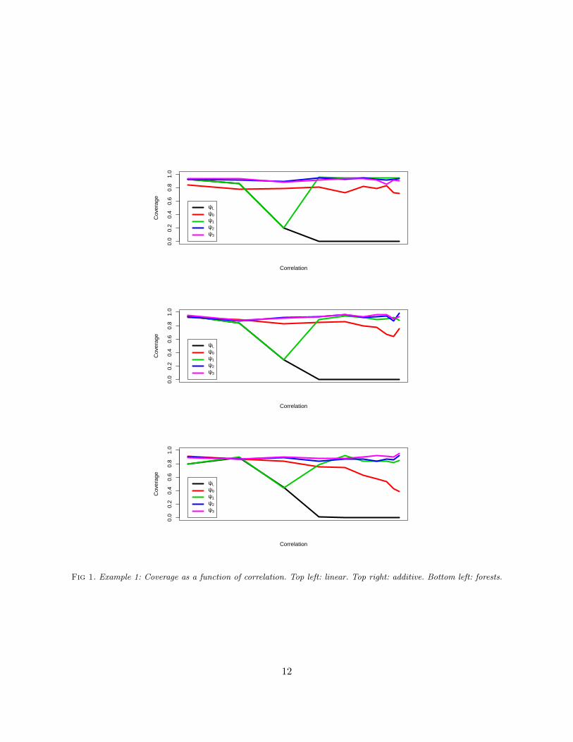
Example 1. We start with a very simple scenario where Y = 2X + ε, ε ∼ N(0, 1), Z1 = δX + ξ,ξ ∼ N(0, 1), and (Z2, . . . , Z5) ∼ N(0, I). Figure 1 shows the coverage as a function of the correlationbetween X and Z1. As expected, ψL has poor coverage as the correlation increases. The parameterψ0 partially corrects the correlation bias while the other parameters do a much better job.

Examples 2-5. Now we consider four multivariate examples. In each case, n = 10, 000, h = 5 andε ∼ N(0, 1). The distributions are defined as follows:

Example 2: X is standard Normal, Z1 = X + N(0, .42), (Z2, . . . , Zh) is standard multivariateNormal. The regression function is Y = 2X3 + ε.

Example 3: Here, Z ∼ N(0, I), X1 = 2Z1 + ε1, X2 = 2Z2 + ε2, Y = 2X1X2 + ε where ε, ε1, ε2 ∼N(0, 1).

Example 4: Let X ∼ Unif(−1, 1), Z ∼ Unif(−1, 1), and Y = X2(X + (7/5)) + (25/9)Z2 + ε. Thisexample is from Williamson et al. (2021). Our coverage for ψL is similar but slightly less than thatin Williamson et al. (2021) but we are using a different nonparametric estimator.

10

Linear Additive ForestψL ψ0 ψ1 ψ2 ψ3 ψL ψ0 ψ1 ψ2 ψ3 ψL ψ0 ψ1 ψ2 ψ3

Example 2 1 0.84 1 1 1.00 0.00 0.79 1.00 1.00 0.97 0.00 0.75 1.00 0.99 0.30Example 3 0 0.00 0 0 0.99 0.00 0.88 0.00 0.00 0.92 0.00 0.00 0.00 0.00 0.91Example 4 1 0.87 1 1 1.00 0.98 0.20 0.98 0.98 0.98 0.00 0.21 0.00 0.86 0.85Example 5 0 0.01 0 0 0.00 0.00 0.83 0.00 0.00 0.85 0.00 0.05 0.00 0.00 1.00

Table 2Coverage results for Examples 2,3,4 and 5. Overall, ψ3 performs best in these examples. But when linear regressions

are used, ψ3 fails. For random forests, ψ3 does poorly in Example 2. The most robust behavior is given by theadditive model.

Example 5: X ∼ N(0, 1), Z1 = X +N(0, .42) (Z2, . . . , Zd) ∼ N(0, I) and Y = 2X2 +XZ1 + ε.

In examples 2,4 and 5, we replaced X with orthogonal polynomials b1(X), b2(X), b3(X).

The results from 100 simulations are summarized in Table 2. Figure 2 shows the average of the leftand right endpoints of the confidence intervals. The first thing to notice is that no method doesuniformly well. Estimating variable importance well is surprisingly difficult. Generally, we find thatψ3 works best. However, it does poorly in two cases: in Example 5, with linear regressions, andin Example 2 using random forests. ψ0 rarely does well. Apparently, the functional is too difficultto estimate nonparametrically. ψ1 works well in a few cases, but is not reliable enough in general.Similar behavior occurs for ψ2. Except for a few cases, ψL never does well. This is not unexpecteddue to the correlation bias. However, it should be noted that these methods are likely all doingwell in the sense of covering the value of ψ in the projected model. For example, when using linearmodels for µ and ν, we are really estimating the value of ψ for the projection of the distributiononto the space of linear models. The parameter estimate may capture useful information even if itis not estimating ψ0.

5. Other Issues

In this section we discuss two further topics: other variable importance parameters, and Shapleyvalues.

5.1. Other Parameters

We have focused on LOCO in this paper but there are many other variable importance parametersall of which can be estimated in a manner similar to the methods in this paper. Samarov (1993)suggested ψ =

∫(∂µ(x, z)/∂x)T (∂µ(x, z)/∂x)dP . This parameter is not subject to correlation bias.

Estimating derivatives can be difficult but in the semiparametric case, ψ takes a simple form. Inthe partially linear model we have ψ = ||β||2 and in the partially linear model with interactions (5)we have

ψ = ||β||2 + 2βGTmZ +GTΣZG

where Gjk = γjk.

11

0.0

0.2

0.4

0.6

0.8

1.0

Correlation

Cov

erag

e

ψL

ψ0

ψ1

ψ2

ψ3

0.0

0.2

0.4

0.6

0.8

1.0

Correlation

Cov

erag

e

ψL

ψ0

ψ1

ψ2

ψ3

0.0

0.2

0.4

0.6

0.8

1.0

Correlation

Cov

erag

e

ψL

ψ0

ψ1

ψ2

ψ3

Fig 1. Example 1: Coverage as a function of correlation. Top left: linear. Top right: additive. Bottom left: forests.

12

0 1 2 3 4 5

0 1 2 3 4 5 6

1.0 1.2 1.4 1.6 1.8 2.0

0 1 2 3 4

ψ3

ψ2

ψ1

ψ0

ψL

Fig 2. The average of the left and right endpoints of the confidence intervals over 100 simulations for Examples2,3,4,5. For each group of three line segments, the top is based on linear models, the middle is based on additivemodels and the bottom is based on random forests.

13

Another parameter is inspired by causal inference. If we viewed X as a treatment and Z as con-founding variables, then (under some conditions) the causal effect, that is the mean of Y had Xbeen set to x, is given by Robins’ g-formula g(x) =

∫µ(x, z)dP (z). We could then define ψ as

the variance Var[g(X)] or the average squared derivative of∫

(∂g(x)/∂x)T (∂g(x)/∂x)dP . Theseparameters do not suffer from correlation bias. Now Var[g(X)] equals βTΣXβ under the partiallylinear model and is (β + ΓmZ)TΣX(β + ΓmZ) under the partially linear model with interactions.Using the derivative, in the partially linear model we get ψ = ||β||2 and in partially linear modelwith interactions we get

ψ = ||β||2 + 2βΓTmZ + ΓTmZmTZΓ.

The nonparametric partial correlation is defined by

ρ =E[(Y − µ(Z))(X − ν(Z))]√E(Y − µ(Z))2E(X − ν(Z))2

.

Under p0 we get a decorrelated version

ρ0 =E0[(Y − µ0(Z))(X − ν0(Z))]√E0(Y − µ0(Z))2E0(X − ν0(Z))2

=

∫ ∫(µ(x, z)− µ0(z))(x−mX)p(x)p(z)dxdz

σX

√∫ ∫ ∫(y − µ0(z))2p(y|x, z)p(x)p(z)

.

More detail about ρ0 are in the appendix.

5.2. Shapley Values

A method for defining variable importance that has attracted much attention lately is based onShapley values (Messalas, Kanellopoulos and Makris, 2019; Aas, Jullum and Løland, 2019; Lundbergand Lee, 2016; Covert, Lundberg and Lee, 2020; Fryer, Strumke and Nguyen, 2020; Covert and Lee,2020; Israeli, 2007; Mase, Owen and Seiler, 2019; Benard et al., 2021). This is an idea from gametheory where the goal is to define the importance of each player in a cooperative game. WhileShapley values can be useful in some settings, for example, computer experiments (Owen andPrieur, 2017) we argue here that Shapley values do not solve the decorrelation issue and LOCO ordecorrelated LOCO may be preferable for routine regression problems. However, this is an activearea of research and the issue is far from settled. Shapley values may indeed have some otheradvantages.

The Shapley value is defined as follows. Suppose we have covariates (Z1, . . . , Zd) and that we wantto measure the importance of Zj . For any subset S ⊂ 1, . . . , d let ZS = (Zj : j ∈ S) and letµ(S) = E[Y |ZS ]. The Shapley value for Zj is

sj =1

d!

∑π

[V (S+j (π))− V (Sj(π))]

where the sum is over of permutations of (Z1, . . . , Zd), Sj(π) denotes all variables before Zj inpermutation π, S+

j (π) = Sj(π)⋃j and V (S) is some measure of fit the regression model with

variables S. If V (S) = −E[(Y − µ(S))2], then

sj =1

d!

∑π

E[(µ(Sj)− µ(S+j ))2].

14

This is just the LOCO parameter averaged over all possible submodels. The Shapley value for agroup of variables can be defined similarly.

It is clear that this parameter is difficult to compute and inference, while possible (Williamson andFeng, 2020) is very challenging. The appeal of the Shapley value is that it has the following niceproperties:

(A1):∑

j sj = E[(Y − µ(Z))2].

(A2) If E[(Y − µ(S⋃i))2] = E[(Y − µ(S

⋃j))2] for every S not containing i or j, then si = sj .

(A3) If we treat Zj , Zk as one variable, then its Shapley value sjk satisfies sjk = sj + sk.

(A4) If E[(Y − µ(S⋃j))2] = E[(Y − µ(S))2] for all S then sj = 0.

However, we see two problems with Shapley values in regression problems. First, it defines variableimportance with respect to all submodels. But most of those submodels are not of interest. Indeed,most of them would be a bad fit to the data and are not relevant. So it is not clear why we shouldinvolve them in any definition of variable importance or in the axioms. (An intriguing idea might beto weight the submodels according to their predictive value.) Second, they succumb to correlationbias. To see this, suppose that Y = βZ1 + ε, that the Zj ’s have variance 1 and that they areperfectly correlated, that is, P (Zj = Zk) = 1 for every j and k. The Shapley value for Z1 turnsout to be s1 = β2/d which is close to 0 when d is large. In contrast, ψ0 = β2 which seems moreappropriate. The confidence interval for ψ0 would have infinite length since the design is singularwhich also seems appropriate since estimating the importance of a single variable among a set ofperfectly correlated variables should be an impossible inferential task. For these reasons, we feelthat decorrelated LOCO may have some advantages over Shapley values.

6. A Balancing Approach

In this section, we briefly outline a different approach to decorrelation based on the idea of balancingfrom causal inference (Imai and Ratkovic, 2014; Fong, Hazlett and Imai, 2018; Ning, Sida and Imai,2020). The idea is to write the decorrelated density as p(x)p(z) = w(x, z)p(x, z) where w(x, z) =p(z)/p(z|x). If we knew w, we could simply apply LOCO using weights Wi = w(Xi, Zi). Now letH = h1, . . . , hk be a set of functions where hj(x, z) = fj(x)gj(z). Then

µj ≡ E[fj(X)]E[gj(Z)] =

∫ ∫hj(x, z)p(x)p(z)dxdz =

∫ ∫w(x, z)dP (x, z).

Now we estimate µj by

µj =1

n

∑i

fj(Xi)1

n

∑i

gj(Zi)

and we estimate∫ ∫

w(x, z)dP (x, z) by

1

n

∑i

Wihj(Xi, Zi).

15

This leads to the set of equations

µj =1

n

∑i

Wihj(Xi, Zi), j = 1, . . . , k.

This does not completely specify W1, . . . ,Wn but we can proceed as follows. We choose W tominimize ||W − W ||2 subject to n−1

∑i Wi = 1 and the above moment constraints. We define

h1(x, z) = 1 so that the constraint n−1∑

i Wi = 1 is included in the moment constraints. Thesolution is

W = 1−Hλ

where 1 = (1, . . . , 1), H is the n× k matrix with Hij = hj(Xi, Zi),

λ = (n−1HTH)−1(h− µ)

and h = n−1(∑

i h1(Xi, Zi), . . . ,∑

i hk(Xi, Zi)). The LOCO parameter and the regressions µ(x, z)and µ(z) are all estimated using the weights. Space does not permit a full examination of thisapproach; we will report more details elsewhere.

7. Conclusion

We showed that correlation bias can be removed from LOCO by modifying the definition appropri-ately. This leads to the parameter ψ0. As we have seen, getting valid inferences for ψ0 nonparamet-rically is difficult even in fairly simple examples. This is mainly because the parameter involves thefunction µ0(z) =

∫µ(x, z)p(x)dx which requires estimating µ(x, z) in regions where there is little

data due to the dependence between x and z.

The easiest remedy is to remove correlated variables as we did for ψ1 but this led to disappointingbehavior. The other remedy was to use a semiparametric model for µ(x, z) which led to ψ2 andψ3. This appears to be the best approach. We emphasize that even when the coverage for ψ2 andψ3 is low, (when the semiparametric model is misspecified), these parameters are still useful ifwe interpret them as projections. For example, ψ2 measures the variable importance of X in theregression function of the form βx + f(z) that best approximates µ(x, z). In the sense ψ2 stillcaptures part of the variable importance. Graham and de Xavier Pinto (2021) discuss in detail theinterpretation of misspecified semiparametric models.

We only dealt with low dimensional models. The methods extends to high dimensional models byusing the usual sparsity based estimators for the nuisance functions µ(z) and ν(z). We plan toexplore this in future work.

Finally, we briefly discussed the role of Shapley values which have become popular in the literatureon variable importance. The motivation for using Shapley values appears to be correlation bias.Indeed, if the variables were independent, Shapley values would probably not be considered. Butwe argued that they do not adequately address the problem. Instead, we believe that some form ofdecorrelation might be preferred.

16

8. Appendix

In this appendix we have proofs and details for a few other parameters.

8.1. Proofs

Theorem 1. Let ψ0(µ, p) =∫ ∫

(µ(x, z)− µ0(z))2p(x)p(z)dxdz. The efficient influence function is

φ(X,Y, Z, µ, p) =

∫(µ(x, Z)− µ0(Z))2p(x)dx+

∫(µ(X, z)− µ0(z))2p(z)dz

+ 2p(X)p(Z)

p(X,Z)(µ(X,Z)− µ0(Z))(Y − µ(X,Z))− 2ψ(p).

In particular, we have the following von Mises expansion

ψ0(µ, p) = ψ0(µ, p) +

∫ ∫φ(x, y, z, µ, p)dP (x, y, z) +R

where the remainder R satisfies

||R|| = O(||p(x, z)− p(x, z)||2) +O(||µ(x, z)− µ(x, z)||2)

+O(||p(x, z)− p(x, z)|| × ||µ(x, z)− µ(x, z)||).

Proof. To show that φ(X,Y, Z, µ, p) is the efficient influence function we verify that φ(X,Y, Z, µ, p)is the Gateuax derivative of ψ and that it has the claimed second order remainder. We will use thesymbol ′ to denote the Gateuax derivative defined by

limε→0

ψ0((1− ε)P + εδXY Z)− ψ0(P )

ε

where δXY Z is a point mass at (X,Y, Z). Also, let δX denote a point mass at X, δXY a point massat (X,Y ) etc. Let w(x, z) = p(x)p(z). Then ψ0 =

∫ ∫(µ(x, z)− µ0(z))2w(x, z)dxdz. Now

ψ′ =

∫ ∫(µ(x, z)− µ0(z))2w′(x, z)dxdz + 2

∫ ∫w(x, z)(µ(x, z)− µ0(z))(µ′(x, z)− µ′0(z))dxdz

First, note that w′(x, z) = p(x)(δZ(z)− p(z)) + p(z)(δX(x)− p(x)). Next

µ(x, z) =

∫yp(y|x, z)dy =

∫yp(x, y, z)

p(x, z)dy

and

µε(x, z) =

∫yp(x, y, z) + ε(δXY Z − p(x, y, z))p(x, z) + ε(δXZ − p(x, z))

dy

17

So

µ′(x, z) =

∫y

p(x, z)(δXY Z − p(x, y, z))− p(x, y, z)(δXZ − p(x, z))

p2(x, z)

dy

=Y

p(X,Z)I(x = X, z = Z)− µ(x, z)− µ(x, z)I(x = X, z = Z)

p(x, z)+ µ(x, z)

=(Y − µ(x, z))

p(x, z)I(x = X, z = Z)

Now µ0(z) =∫µ(x, z)p(x)dx so

µ′0(z) =

∫µ(x, z)(δX(x)− p(x))dx+

∫p(x)µ′(x, z)dx

= µ(X, z)− µ0(z) +(Y − µ(X, z))p(X)

p(X, z)I(z = Z)

so

φ(X,Y, Z, µ, p) =

∫(µ(x, Z)− µ0(Z))2p(x)dx− ψ +

∫(µ(X, z)− µ0(z))2p(z)dz − ψ

+ 2w(X,Z)(µ(X,Z)− µ0(Z))(Y − µ(X,Z))

p(X,Z)

− 2

∫ ∫w(x, z)(µ(x, z)− µ0(z))(µ(X, z)− µ0(z))dxdz

− 2(Y − µ(X,Z))p(X)

p(X,Z)

∫w(x, Z)(µ(x, Z)− µ0(Z))dx

=

∫(µ(x, Z)− µ0(Z))2p(x)dx+

∫(µ(X, z)− µ0(z))2p(z)dz − 2ψ

+ 2w(X,Z)(µ(X,Z)− µ0(Z))(Y − µ(X,Z))

p(X,Z)

− 2

∫ ∫w(x, z)(µ(x, z)− µ0(z))(µ(X, z)− µ0(z))dxdz

− 2(Y − µ(X,Z))p(X)p(Z)

p(X,Z)

∫p(x)(µ(x, Z)− µ0(Z))dx

=

∫(µ(x, Z)− µ0(Z))2p(x)dx+

∫(µ(X, z)− µ0(z))2p(z)dz

+ 2p(X)p(Z)

p(X,Z)(µ(X,Z)− µ0(Z))(Y − µ(X,Z))− 2ψ(p)

which has the claimed form.

Now we consider the von Mises remainder. The remainder at (p, µ) in the direction of (p, µ) is

R = ψ(p, µ)− ψ(p, µ)−∫φ(u, µ, p)dP (u).

18

Now

−R = ψ(p, µ)− ψ(p, µ)

+

∫ ∫p(x)p(z)(µ(x, z)− µ0(z))2dxdz +

∫ ∫p(x)p(z)(µ(x, z)− µ0(z))2dxdz

+ 2

∫ ∫ ∫p(x, y, z)

p(x)p(z)

p(x, z)(µ(x, z)− µ0(z))(y − µ(x, z))dxdydz − 2ψ(p)

=

∫ ∫p(x)p(z)(µ(x, z)− µ0(z))2dxdz +

∫ ∫p(x)p(z)(µ(x, z)− µ0(z))2dxdz

+ 2

∫ ∫ ∫p(x, y, z)

p(x)p(z)

p(x, z)(µ(x, z)− µ0(z))(y − µ(x, z))dxdydz

− ψ(p, µ)− ψ(p, µ)

=

∫ ∫p(x)p(z)(µ(x, z)− µ0(z))2dxdz +

∫ ∫p(x)p(z)(µ(x, z)− µ0(z))2dxdz

+ 2

∫ ∫p(x, z)

p(x)p(z)

p(x, z)(µ(x, z)− µ0(z))(µ(x, z)− µ(x, z))dxdz

− ψ(p, µ)− ψ(p, µ)

=

∫ ∫p(x)p(z)(µ(x, z)− µ0(z))2dxdz +

∫ ∫p(x)p(z)(µ(x, z)− µ0(z))2dxdz

+ 2

∫ ∫p(x)p(z)(µ(x, z)− µ0(z))(µ(x, z)− µ(x, z))dxdz

−∫ ∫

p(x)p(z)(µ(x, z)− µ0(z))2dxdz −∫ ∫

p(x)p(z)(µ− µ0)2dxdz + 2S

where

S = 2

∫ ∫(p(x, z)− p(x, z))(µ(x, z)− µ(x, z))p(x)p(z)(µ(x, z)− µ0(z))dxdz.

Now consider the term m =∫ ∫

p(x)p(z)(µ(x, z)− µ0(z))(µ(x, z)− µ(x, z))dxdz. We have

m =

∫ ∫p(x)p(z)(µ(x, z)− µ0(z))(µ(x, z)− µ(x, z))dxdz

=

∫ ∫p(x)p(z)(µ(x, z)− µ0(z))(µ(x, z)− µ0(z) + µ0(z)− µ0(z) + µ0(z)− µ(x, z))dxdz

=

∫ ∫p(x)p(z)(µ(x, z)− µ0(z))(µ(x, z)− µ0(z))dxdz +

∫ ∫p(x)p(z)(µ(x, z)− µ0(z))(µ0(z)− µ0(z))dxdz

+

∫ ∫p(x)p(z)(µ(x, z)− µ0(z))(µ0(z)− µ(x, z))dxdz

=

∫ ∫p(x)p(z)

√δ√δdxdz + 0−

∫ ∫p(x)p(z)δdxdz

19

where δ = µ(x, z)− µ0(z) and δ = µ(x, z)− µ0(z). Hence,

−R =

∫ ∫p(x)p(z)δdxdz +

∫ ∫p(x)p(z)δdxdz + 2

∫ ∫p(x)p(z)

√δ√δdxdz

− 2

∫ ∫p(x)p(z)δdxdz −

∫ ∫p(x)p(z)δdxdz

−∫ ∫

p(x)p(z)δdxdz −∫ ∫

p(x)p(z)δdxdz +

∫ ∫p(x)p(z)δdxdz

=

∫ ∫p(x)p(z)δdxdz +

∫ ∫p(x)p(z)δdxdz −

∫ ∫p(x)p(z)(

√δ −√δ)2dxdz

− 2

∫ ∫p(x)p(z)δdxdz −

∫ ∫p(x)p(z)δdxdz +

∫ ∫p(x)p(z)δdxdz

=

∫ ∫(p(x)− p(x))p(z)(δ − δ)dxdz +

∫ ∫p(x)(p(z)− p(z))(δ − δ)dxdz

+

∫ ∫(p(x)− p(x))(p(z)− p(z))δdxdz −

∫ ∫p(x)p(z)(

√δ −√δ)2dxdz.

And hence

||R|| = O(||p(x)− p(x)|| ||δ − δ||) +O(||p(z)− p(z)|| ||δ − δ||)+O(||p(x)− p(x)|| ||p(z)− p(z)||) +O(||δ − δ||2)

= O(||p(x, z)− p(x, z)||2) +O(||µ(x, z)− µ(x, z)||2)

+O(||p(x, z)− p(x, z)|| × ||µ(x, z)− µ(x, z)||).

Lemma 3. Suppose that ||µ(x, v) − µ(x, v)|| = oP (n−1/4). Then, when ψ1 6= 0, we have that√n(ψ1 − ψ1) N(0, τ2) for some τ2.

Proof. We have

Yi − µ(Vi) = (Yi − µ(Vi)) + (µ(Vi)− µ(Vi)) + (µ(Vi)− µ(Vi))

= (Yi − µ(Vi))− (Vi − Vi)T∇µ(Vi) + (µ(Vi)− µ(Vi))

for some Vi between Vi and Vi. Squaring, summing and letting εi = Yi − µ(Vi),

1

n

∑i

(Yi − µ(Vi))2 =

1

n

∑i

ε2i +1

n

∑i

((Vi − Vi)T∇µ(Vi))2 +

1

n

∑i

(µ(Vi)− µ(Vi))

+2

n

∑i

εi(Vi − Vi)T∇µ(Vi)2 +

2

n

∑i

εi(µ(Vi)− µ(Vi))

+2

n(Vi − Vi)T∇µ(Vi)(µ(Vi)− µ(Vi))

=1

n

∑i

ε2i +2

n

∑i

εi(Vi − Vi)T∇µ(Vi) +2

n

∑i

εi(µ(Vi)− µ(Vi)) +Rn

20

where Rn = O(||δ− δ||2) +O(||µ− µ||2) +O(||δ− δ|| ||µ− µ||2) = oP (n−1/2). The mean of the firstthree terms is E[(Y − µ(V ))2]. By a similar argument,

1

n

∑i

(Yi − µ(Xi, Vi))2 =

1

n

∑i

ε2i +2

n

∑i

εi(Vi − Vi)T∇µ(Xi, Vi)

+2

n

∑i

εi(µ(Xi, Vi)− µ(Xi, Vi)) + Rn

where εi = Yi − µ(Xi, Vi), Rn = O(||δ − δ||2) + O(||µ − µ||2) + O(||δ − δ|| ||µ − µ||2) = oP (n−1/2)and the mean of the first three terms is E[(Y − µ(X,V ))2]. The result follows from the CLT andthe fact that

√n(Rn + Rn) = oP (1).

Lemma 4. We have that ψ0 under the partially linear model with interactions, is equal to ψ3 =θTΩθ where

Ω = ΣX ⊗(

1 mTZ

mZ ΣZ

).

Proof. Let us write

µ(x, z) = θTW ≡ θT0 X +

h∑j=1

θTj XZj

where we have written θ = (θ0, θ1, . . . , θh) and so µ0(z) = θT0 mX +∑h

j=1 θTj mXZj . Thus

(µ(x, z)− µ0(z))2 = θT0 (X −mX)(X −mX)T θ0 +h∑j=1

θTj (X −mX)(X −mX)TZ2j θj

+ 2h∑j=1

θT0 (X −mX)(X −mX)TZjθj + 2∑j 6=k

θTj (X −mX)(X −mX)TZjZkθk

and so

E0[(µ(x, z)− µ0(z))2] = θTΣXθ0 +h∑j=1

θTj ΣX(ΣZ(j, j) +m2Z(j))θj

+ 2

h∑j=1

θT0 ΣXmZ(j)θj + 2∑j 6=k

θTj θk(ΣZ(j, k) +mZ(j)mZ(k))

= θTΩθ.

8.2. ψL Under the Semiparametric Model

Here we give the form that ψL takes under the semiparametric model. Under the model µ(x, z) =f(z) + xTβ(z), we have ψL = E[βT (Z)(X − ν(Z))(X − ν(Z))Tβ(Z)] which has efficient influencefunction

φ = 2β(Z)T (X − ν(Z))(X − ν(Z))TV −1(Z)XY

− 2β(Z)T (X − ν(Z))(X − ν(Z))TV −1(Z)(X − ν(Z))(X − ν(Z))Tβ

− βT (X − ν(Z))(X − ν(Z))Tβ − ψL.21

When µ(x, z) = βTx+∑

jk γjkxjzk + f(z) then

ψL = θT (Ω11 + Ω12 + Ω21 + Ω22)

where

Ω11 =

(1 mT

Z

mZ ΣZ +mZmTZ

)⊗ ΣX ,

Ω12 =

(1 mT

Z

mZ ΣZ +mZmTZ

)⊗ E[(X −mX)(mX − ν(Z))T ],

Ω21 =

(1 mT

Z

mZ ΣZ +mZmTZ

)⊗ E[(X −mX)(mX − ν(Z))T ],

Ω12 =

(1 mT

Z

mZ ΣZ +mZmTZ

)⊗ E[(mX − ν(Z))(X −mX)T ],

Ω22 =

(1 mT

Z

mZ ΣZ +mZmTZ

)⊗ E[(mX − ν(Z))(mX − ν(Z))T ].

We omit the expression for influence function.

8.3. Partial Correlation

In this section, we give the decorrelated version of the partial correlation. Recall that

ρ0 =E0[(Y − µ0(Z))(X − ν0(Z))]√E0(Y − µ0(Z))2E0(X − ν0(Z))2

=

∫ ∫(µ(x, z)− µ0(z))(x−mX)p(x)p(z)dxdz

σX

√∫ ∫ ∫(y − µ ∗ (z))2p(y|x, z)p(x)p(z)

.

Theorem 5 The efficient influence function for ρ0 is

φ =1√φ2φ3

φ1 −

ψ1

2ψ2φ2 −

ψ2

2ψ3φ3

where, in this section, we define

ψ1 =

∫ ∫(µ(x, z)− µ0(z))(x−mX)p(x)p(z)dxdz

ψ2 = σ2X

ψ3 =

∫ ∫ ∫(y − µ0(z))2p(y|x, z)p(x)p(z)dxdzdy

and

φ1 = µ0(X)(X −m) + (X −m)Y − µ(X,Z)

p(X,Z)p(X)p(Z) + (X −m)p(X)µ(X,Z)− µ0(z)− 2ψ1

φ2 = (X −m)2 − σ2X

φ3 = (Y − v(Z))2 − ψ3 − 2p(X)p(Z)

p(X,Z)(Y − µ(X,Z)).

22

Proof. Let us write ρ0 = f(ψ1, ψ2, ψ3) where f(a, b, c) = a/√bc and

ψ1 = E0[(Y − µ0(Z))(X − ν0(Z))]

ψ2 = σ2X

ψ3 =

∫ ∫ ∫(y − µ ∗ (z))2p(y|x, z)p(x)p(z).

So the influence function is

f1(ψ1, ψ2, ψ3)φ1 + f2(ψ1, ψ2, ψ3)φ2 + f3(ψ1, ψ2, ψ3)φ3

where fj = ∂f/∂ψj and φj is the influence function for ψj . Hence,

φ =1√φ2φ3

φ1 −

ψ1

2ψ2φ2 −

ψ2

2ψ3φ3

.

Now

ψ1 =

∫(µ0(x)− ψ0)(x−mX)p(x)dx =

∫µ0(x)(x−mX)p(x)dx

where µ0(x) =∫µ(x, z)p(z). So

φ1 =

∫µ0(x)′(x−mX)p(x)dx−

∫µ0(x)m′Xp(x)dx+

∫µ0(x)(x−mX)p(x)′dx

=

∫µ0(x)′(x−mX)p(x)dx−

∫µ0(x)(X −mX)p(x)dx+ µ0(X)(X −mX)− ψ1

= µ0(X)(X −mX) +

∫µ0(x)′(x−mX)p(x)dx− 2ψ1.

Now

µ0(x)′ =

∫µ′(x, z)p(z)dz + µ(x, Z)− µ0(z)

=

∫Y − µ(x, z)

p(x, z)I(X = x, Z = z)p(z)dz + µ(x, Z)− µ0(z)

= I(x = X)Y − µ(x, Z)

p(x, Z)p(Z) + µ(x, Z)− µ0(z).

Thus ∫(x−m)p(x)

I(x = X)

Y − µ(x, Z)

p(x, Z)p(Z) + µ(x, Z)− µ0(z)

(X −m)Y − µ(X,Z)

p(X,Z)p(X)p(Z) + (X −m)p(X)µ(X,Z)− µ0(z)

So

φ1 = µ0(X)(X −m) + (X −m)Y − µ(X,Z)

p(X,Z)p(X)p(Z) + (X −m)p(X)µ(X,Z)− µ0(z)− 2ψ1.

23

Alsoφ2 = (X −m)2 − σ2.

Now we turn to ψ3 =∫ ∫ ∫

(y − µ ∗ (z))2p(x, y, z). Then

φ3 = (Y − v(Z))2 − ψ3 − 2

∫p(x, y, z)(y − v(z))v′(z)dz

= (Y − v(Z))2 − ψ3 − 2

∫p(x, z)(µ− v(z))v′(z)dz

and

v′(z) = µ(X, z)− v(z) + I(z = Z)p(X)(Y − µ(X, z))

p(X, z)

so that

φ3 = (Y − v(Z))2 − ψ3 − 2

∫p(x, z)(µ− v(z))v′(z)dz

= (Y − v(Z))2 − ψ3 − 2p(X)p(Z)

p(X,Z)(Y − µ(X,Z)).

The remainder can be shown to be second order in a similar way to ψ0. We omit the details.

8.4. Varying Coefficient Model

Let µ(x, z) = xTβ(z) + f(z). In this case ψ0 becomes ψ4 = tr(ΣXH). Define

V (z) = Var[X|Z = z] C(z) = Cov[X,Y |Z = z] f(z) = µ(z)− ν(z)Tβ(z)

β(z) = V −1(Z)C(z) M = E[β(Z)] S = Var[β(Z)].

Lemma 6 The efficient influence function for ψ4 is

φ = tr(ΣXφH) + (X −mX)TH(X −m)− ψ4

where H = E[β(Z)β(Z)T ],

φH = β(Z)β(Z)T −H + β(Z)[Y XT − β(Z)T (X − ν(Z))(X − ν(Z))T ]V −1(Z)

+ V −1(Z)[XY − (X − ν(Z))(X − ν(Z))Tβ(Z)]β(Z)T .

Hence, the estimator is

ψ4 =1

n

∑i

tr(ΣX φH(Ui)) +1

n

∑i

(Xi −X)TH(Ui)(Xi −X).

24

References

Aas, K., Jullum, M. and Løland, A. (2019). Explaining individual predictions when features aredependent: More accurate approximations to Shapley values. arXiv preprint arXiv:1903.10464.

Benard, C., Biau, G., Da Veiga, S. and Scornet, E. (2021). SHAFF: Fast and consistentSHApley eFfect estimates via random Forests. arXiv preprint arXiv:2105.11724.

Covert, I. and Lee, S.-I. (2020). Improving kernelshap: Practical shapley value estimation vialinear regression. arXiv preprint arXiv:2012.01536.

Covert, I., Lundberg, S. and Lee, S.-I. (2020). Understanding global feature contributionswith additive importance measures. arXiv preprint arXiv:2004.00668.

Dai, B., Shen, X. and Pan, W. (2021). Significance tests of feature relevance for a blackboxlearner. arXiv preprint arXiv:2103.04985.

D’Amour, A., Ding, P., Feller, A., Lei, L. and Sekhon, J. (2021). Overlap in observationalstudies with high-dimensional covariates. Journal of Econometrics 221 644–654.

Fong, C., Hazlett, C. and Imai, K. (2018). Covariate balancing propensity score for a continuoustreatment: Application to the efficacy of political advertisements. The Annals of Applied Statistics12 156–177.

Fryer, D., Strumke, I. and Nguyen, H. (2020). Shapley value confidence intervals for variableselection in regression models.

Graham, B. S. and de Xavier Pinto, C. C. (2021). Semiparametrically efficient estimation ofthe average linear regression function. Journal of Econometrics.

Gretton, A., Borgwardt, K. M., Rasch, M. J., Scholkopf, B. and Smola, A. (2012). Akernel two-sample test. The Journal of Machine Learning Research 13 723–773.

Hines, O., Dukes, O., Diaz-Ordaz, K. and Vansteelandt, S. (2021). Demystifying statisticallearning based on efficient influence functions. arXiv preprint arXiv:2107.00681.

Ibragimov, R. and Muller, U. K. (2010). t-Statistic based correlation and heterogeneity robustinference. Journal of Business & Economic Statistics 28 453–468.

Imai, K. and Ratkovic, M. (2014). Covariate balancing propensity score. Journal of the RoyalStatistical Society: Series B (Statistical Methodology) 76 243–263.

Israeli, O. (2007). A Shapley-based decomposition of the R-square of a linear regression. TheJournal of Economic Inequality 5 199–212.

Lei, J., G’Sell, M., Rinaldo, A., Tibshirani, R. J. and Wasserman, L. (2018). Distribution-free predictive inference for regression. Journal of the American Statistical Association 113 1094–1111.

Lundberg, S. and Lee, S.-I. (2016). An unexpected unity among methods for interpreting modelpredictions. arXiv preprint arXiv:1611.07478.

Mase, M., Owen, A. B. and Seiler, B. (2019). Explaining black box decisions by shapley cohortrefinement. arXiv preprint arXiv:1911.00467.

Messalas, A., Kanellopoulos, Y. and Makris, C. (2019). Model-agnostic interpretability withshapley values. In 2019 10th International Conference on Information, Intelligence, Systems andApplications (IISA) 1–7. IEEE.

Newey, W. K. and Robins, J. R. (2018). Cross-fitting and fast remainder rates for semiparametricestimation. arXiv preprint arXiv:1801.09138.

Ning, Y., Sida, P. and Imai, K. (2020). Robust estimation of causal effects via a high-dimensionalcovariate balancing propensity score. Biometrika 107 533–554.

Owen, A. B. and Prieur, C. (2017). On Shapley value for measuring importance of dependentinputs. SIAM/ASA Journal on Uncertainty Quantification 5 986–1002.

25

Ribeiro, M. T., Singh, S. and Guestrin, C. (2016). Model-agnostic interpretability of machinelearning. arXiv preprint arXiv:1606.05386.

Rinaldo, A., Wasserman, L. and G’Sell, M. (2019). Bootstrapping and sample splitting forhigh-dimensional, assumption-lean inference. The Annals of Statistics 47 3438–3469.

Samarov, A. M. (1993). Exploring regression structure using nonparametric functional estimation.Journal of the American Statistical Association 88 836–847.

Sani, N., Lee, J., Nabi, R. and Shpitser, I. (2020). A Semiparametric Approach to InterpretableMachine Learning. arXiv preprint arXiv:2006.04732.

Sejdinovic, D., Sriperumbudur, B., Gretton, A. and Fukumizu, K. (2013). Equivalence ofdistance-based and RKHS-based statistics in hypothesis testing. The Annals of Statistics 2263–2291.

Szekely, G. J., Rizzo, M. L. and Bakirov, N. K. (2007). Measuring and testing dependenceby correlation of distances. The annals of statistics 35 2769–2794.

Williamson, B. and Feng, J. (2020). Efficient nonparametric statistical inference on popula-tion feature importance using Shapley values. In International Conference on Machine Learning10282–10291. PMLR.

Williamson, B. D., Gilbert, P. B., Simon, N. R. and Carone, M. (2020). A unified approachfor inference on algorithm-agnostic variable importance. arXiv preprint arXiv:2004.03683.

Williamson, B. D., Gilbert, P. B., Carone, M. and Simon, N. (2021). Nonparametric variableimportance assessment using machine learning techniques. Biometrics 77 9–22.

Zhang, L. and Janson, L. (2020). Floodgate: inference for model-free variable importance. arXivpreprint arXiv:2007.01283.

26