Deconvolution of Images and Spectra - Robert...

Deconvolutionof Images and Spectra

Second Edition

Edited by

Peter A. JanssonE. I. DU PONT DE NEMOURS AND COMPANY (INC.)

EXPERIMENTAL STATION

WILMINGTON, DELAWARE

0APACADEMIC PRESS

San Diego London BostonNew York Sydney Tokyo Toronto

To my father,the late John H. Jansson,remembered for devotion to his family,and to the advancment of science and education

This book is printed on acid-free paper. @

Copyright 0 1997,1984 by Academic Press, Inc.

All rights reserved.No part of this publication may be reproduced ortransmitted in any form or by any means, electronic ormechanical, including photocopy, recording, or anyinformation storage and retrieval system, withoutpermission in writing from the publisher.

Couer image: See Chapter 7, Figure 14 (page 253). Used with permission.

ACADEMIC PRESS, INC.525 B Street, Suite 1900, San Diego, CA 92101-4495, USA1300 Boylston Street, Chestnut Hill, MA 02167, USAhttp://www.apnet.com

ACADEMIC PRESS, LIMITED24-28 Oval Road, London NW1 7DXhttp://www.hbuk.co.uk/ap/

Library of Congress Cataloging-in-Publication Data

Deconvolution of images and spectra/ edited by Peter A. Jansson.-2nd ed.p. cm.

Rev. ed. of: Deconvolution. 1984.Includes bibliographical references and index.ISBN o-12-380222-9 (alk. paper)1. Spectrum analysis-Deconvolution. I. Jansson, Peter A. II. Deconvolution.

QC4.51.6.D45 1997621.36’ l-dc20

96-27097CIP

Printed in the United States of America96 97 98 99 00 EB 9 8 7 6 5 4 3 2 I

Chapter 14 Alternating Projections ontoConvex Sets

Robert J. Marks II

Depaflment of Elechical Engineering,The University of WashingtonSeattle, Washington

I.II.

III.

IV.

V.VI.

Introduction 478Geometrical POCS 478A. Convex Sets 479B. Projecting onto a Convex Set 480c . POCS 482Convex Sets of Signals 484A. The Signal Space 484B. Some Commonly Used Convex Sets of Signals 486Examples 490A. Von Neumann’s Alternating Projection Theorem 490B. The Papoulis-Gerchberg Algorithm 490C. Howard’s~Minimum-Negativity-Constraint Algorithm 494D. Restoration of Linear Degradation 494Notes 497Conclusions 498References 499

List of Symbols

A,B,C,D,A,,A,,A3Eii,,Z,,&2'-+ +uA, ‘Bu(x), u(x), u,(x), u,(x), w(x), z(x)

m(x)U(w), V(w)POSBEBS

sets of vectors or functionsthe universal setmultidimensional vectorsvectors in the sets A and Bfunctions of a continuous variablethe middle of a signalthe Fourier transforms of u(x) and u(x)positivebounded energybounded signals

476

DECONVOLUTION OF IMAGES AND SPECTRASECOND EDITION

Copyright 0 1997 by Academic Press, Inc.All rights of reproduction in any form reserved.

ISBN: O-12-380222-9

14. Alternating Projections onto Convex Sets 477

CACPLVPPsP,PIIMMBSTTLnXd(x)

a

o(x)

o(qX)

9x projection operator onto a set A,._&) a function in a subspace 9L2 a Hilbert space with continuous variables12 a Hilbert space with discrete variablesu[nl element IZ in a sequence u

constant areaconstant phaselinear varietya projection matrixprojection onto a set Sprojection onto set mpseudo-inversesignals with identical middlesnumber of setsan operatora degradation matrixmatrix transposition (used as a superscript)time limitedbandwidthduration limita displacement function used to define linearvarieties(a) 0 I (Y I 1 parameterizes the line connect-ing two vectors; (b) (Y > 0 is used to define acone in a Hilbert spacerelaxation parameterfinite real numbers used to define a subspacecoordinates on a two-dimensional planeimage and object vectorsthe result of iteration IZ on the restoration of adiscrete objectthe result of iteration k on restoration of anobject, o[ n]an object that is a function of a continuousvariablethe result of iteration N on restoration of anobject of a conea Hilbert spacethe imaginary part ofa subspace (or linear manifold) in a Hilbertspacea projection operatorthe real part ofthe subspace that is the orthogonal comple-ment of 9

478 Robert J. Marks II

P

an identity operatorsetin set notation, read “such that”intersectionis an element of1, or L, normperpendicularthe area of a signal

I. Introduction

Alternating projections onto convex sets (POCS)* [ll is a powerful tool forsignal and image restoration and synthesis. The desirable properties of areconstructed signal may be defined by several convex signal sets, whichmay be further defined by a convex set of constraint parameters. Itera-tively projecting onto these convex constraint sets may result in a signalthat contains all desired properties. Convex signal sets are frequentlyencountered in practice and include the sets of band-limited signals,duration-limited signals, signals that are the same (e.g., zero) on somegiven interval, bounded signals, signals of a given area, and complex signalswith a specified phase.

POCS was initially introduced by Bregman [2] and Gubin et al. [3] andwas later popularized by Youla and Webb [4] and Sezan and Stark [5].POCS has been applied to such topics as sampling theory [6], signalrecovery [7], deconvolution and extrapolation 181, artificial neural networks[9, 10, 11, 12, 131, tomography [l, 14, 151, and time-frequency analysis[16, 171. A superb overview of POCS with other applications is in the bookby Stark [l] and the monograph by Combette [X3].

II. Geometrical POCS

Although signal processing applications of POCS use sets of signals, POCSis best visualized viewing the operations on sets of points. In this section,POCS is introduced geometrically.

*The alternating term is implicit in the POCS paradigm, but traditionally is not includedin the acronym.

14. Alternating Projections onto Convex Sets

Figure 1 The set A is convex. The set B is not. A set is convex if every linesegment with end points in the set is totally subsumed in the set.

A. COiWEX SETS

A set, A, is convex if for every vector ii1 E A and every i& E A, it followsthat (~2~ + (1 - a)Z2 E A for all 0 5 (Y 5 1. In other words, the linesegment connecting iZ1 and iZ2 is totally subsumed in A. If any portion ofthe cord connecting two points lies outside of the set, the set is not convex.This is illustrated in Fig. 1. Examples of geometrical convex sets includeballs, boxes, lines, line segments, cones, and planes.

Closed convex sets are those that contain their boundaries. In twodimensions, for example, the set of points

A, = 1(x, y)lx’ + y2 < 1)

is not closed because the points on the circle x2 + y* = 1 are not in theset. The set

A = {(x,y)lx* +Y* 5 l)

is a closed convex set. A is referred to as the closure of A,. Henceforth, allconvex sets will be considered closed.

Sttictly convex sets are those that do not contain any flat boundaries. Aball is strictly convex whereas a box is not. Neither is a line.’

‘Rigorously, a set A is strictly convex if for any distinct Z1, Zz E A, (Z1 + L&)/2 is aninterior point of A. A vector Z is called an i&e&r point of closed set A if Z E A andZ G Closure[E - A], where E is the universal set. In other words, an interior point does notlie on the boundary of a closed convex set.


Figure 2 The set A is convex. The projection of C onto A is the unique elementin A closest to C.

B. PROJECTING ONTO A CONFEX SET

The projection onto a convex set is illustrated in Fig. 2. For a given v’ P A,the projection onto A is the unique vector ii E A such that the distancebetween ii and u’ is minimum. If v’ E A, then the projection onto A is 5.In other words, the projection and the vector are the same.

Figure 3 Alternating projection between two or more convex sets with nonemptyintersection results in convergence to a fixed point in the intersection. Here, sets A(a Iine segment) and B are convex. InitiaIizing the iteration at $‘) results inconvergence to ZCrn) E A n B.

14. Alternating Projections onto Convex Sets

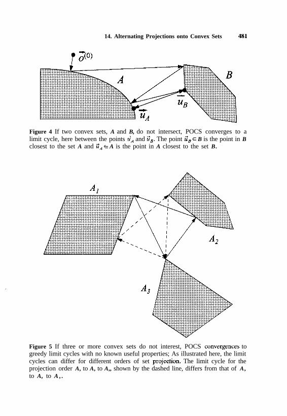
Figure 4 If two convex sets, A and B, do not intersect, POCS converges to alimit cycle, here between the points 7;A and iiB. The point iiB E B is the point in Bclosest to the set A and GA E A is the point in A closest to the set B.

............................................:::::):.):.:.:.:.:.:.:.:.:.:.~:.:.:,:.:.:,: . . . . . . . . . . . . . . . . . . . . . . . . . . . . . . . . . . . . . . . .:.......................................................................................:.:.:.:.:.:.:.:.:.:.:.:.:.:.:.:.:.:.:.:.:.:,:.:.:.:.:.:.:.:.:.:.:.:.:.:.:.:.:.:.:.:.:.:..............................................................................................................................................................................................................................................:::::i::::::::::::::::::::::::::::::::::~::::~...........................................................................................................................................................................................................................................................................................................................................................................................................................................................................................................................................................................................................................................................................................................................................................................................................................................................................................................................................................................................................................................................................................................................................................................................................................................................................................................................................................................................................................................................................................................................................................................................................................................................................................................................................................................................................................................................................................................................................................................................................................................................................................................................................................................................................................................................................................................................................................................................................................................................................................................................................................................................................................................................................................

Figure 5 If three or more convex sets do not interest, POCS convergences togreedy limit cycles with no known useful properties; As illustrated here, the limitcycles can differ for different orders of set proje@on. The limit cycle for theprojection order A, to A, to A,, shown by the dashed line, differs from that of A,to A, to A , .


c. POCS

There are three outcomes in the application of POCS. Each depends onthe various ways that the convex sets intersect.

1. The remarkable primary result of POCS is that, given two or moreconvex sets with nonempty intersection, alternately projecting amongthe sets will converge to a point included in the intersection [l, 41.This is illustrated in Fig. 3. The actual point of convergence willdepend on the initialization unless the intersection is a single point.

2. If two convex sets do not intersect, convergence is to a limit cyclethat is a mean square solution to the problem. Specifically, the cycleis between points in each set that are closest in the mean-squaresense to the other set [19]. This is illustrated in Fig. 4.

3. Conventional POCS breaks down in the important case where threeor more convex sets do not intersect [21]. POCS converges to greedylimit cycles that are dependent on the ordering of the projections anddo not display any desirable optimal&y properties. This is illustratedin Fig. 5.

Figure 6 Here, the sets A and B intersect as do the sets C and D. Shown is oneof the possible greedy limit cycles resulting from application of POCS. The order ofprojection is A to B to C to D. The (convex) intersections, A n B and C n D, areshown shaded. Note, though, a greedy limit cycle between the convex sets A n Band C fl D is also possible when using the projection order A to D to C to B. Theresult is shown by a dashed line. In this case, the limit cycle is akin to that obtainedby application of POCS to two nonintersecting convex sets.


Figure 7 Conventional convex sets can be enlarged (or fuzzified) into fuzzyconvex sets. Here, the three shaded ellipses correspond to nonintersecting convexsets. Each of the three sets is enlarged to the ellipses shown with the long dashedlines. Enlargement can be done by mathematical morphological dilation of theoriginal convex sets. There is still no intersection among these larger sets, so thesets are enlarged again. Intersection now occurs. The resulting dashed lines arecontours, or a-cuts, of fuzzy convex sets. Any group of nonintersecting convex setscan be enlarged sufficiently in this manner so that the enlarged sets (cu-cuts) have afinite intersection. Ideally, the minimum enlargement that produces a nonemptyintersection is used. A point in that intersection is deemed to be “near” each of theconvex sets. In this figure, the point is o cm). This point can be obtained by applyingconventional POCS to the enlarged sets.

This greedy limit cycle can also occur when some of the convex setsintersect and others do not. This is illustrated in Fig. 6.

Oh and Marks [22] have applied Zadeh’s ideas on fuzzy convex sets 1241to the case where the convex sets do not intersect. The idea is to find apoint that is “near” each of the sets.* Three nonintersecting convex setsare shown in Fig. 7. Each of the convex sets is “enlarged” sufficiently sothat the resulting convex sets intersect. + There always exists a degree of

*The term “near” is referred to as a fuzzy linguistic variable.‘The enlargement of the set is obtained by morphological dilution with a convex dilation

kernel set. If the kernel is a circle, dilation can be geometrically viewed as the result of rollingthe circle on the boundary of the convex set. The larger the diameter of the circle, the greaterthe dilation. If both A and the dilation kernel set are convex, then so is the dilation. In Fig. 7,enlargement eventually results in the unique intersection point, oCm). Description of thedetails of this process is beyond the scope of this chapter. Details are in the papers by Oh andMarks (22, 23).


enlargement that results in a nonempty intersection of all of the sets.* Thesmallest enlargement that results in a nonempty intersection is sought. Apoint in the resulting intersection is then “near” each of the convex sets.Conventional POCS is applied to these sets to find such a point.

III. Convex Sets of Signals

The geometrical view introduced in the previous section allows powerfulinterpretation of POCS applied in a signal space, Z? For our notation, wewill use continuous functions, although the concepts can be easily ex-tended to functions in discrete time.”

A. THE SIGNAL SPACE

An image, u(x), is the 2 if**

IMx)ll < a,

where the norm of U(X) is

Ilu(x>ll = {/” lu(x)12 fix.-cc

*Proof: Enlarge each set to fill the whole space.‘More properly, a Hilbert or L, space (20).“That is, from an L, to an 1, space. One advantage of discrete time is the guaranteed

strong convergence of POCS. Denote the nth element of a sequence u by z&r] and let @[n]be the kth POCS iteration. Let o[n] be the point of convergence and u[n] is any point(including the origin) in I,, then

lim I]u[n] - &+[n]]l* = I]u[n] - o[n]]]’k+m

for all u[n]. The square of the I, norm of a sequence u[n] is

llu[n1112 = 2 lu[n112.a= --m

In continuous time, only weak convergence can generally be assured [4]. Specifically,

for all u(x) is L,. Strong convergence assures weak convergence.**Signals in a Hilbert space are also required to be Lebesgue measurable, although this

will not be of concern in our treatment.


The energy of u(x) is

E = llu(x)l12. (1)The signal space thus consists of all finite energy signals. Geometrically,x’ = u(x) can be visualized as a point in the signal space a distance ofIlu(x from the origin, u(x) = 0. Similarly, the (mean square) distancebetween two points U(X) and v(x) is simply Ilu(x> - u(x>ll.

Two objects, W(X) and z(x), are said to be orthogonal if

/m W(X)z*(x> dx = 0, (2)--m

where the superscript asterisk denotes complex conjugation.Some examples of signal sets follow.

1. Convex Sets

Analogous to the definition given for sets of vectors, a set of signals, A, isconvex if, for 0 I (Y I 1, the signal

au,(x) + (1 - a>u,(x> EA (3)

when z+(x), U,(X) E A.

2. Subspaces

Subspaces (also called linear manifolds) can be visualized as hyperplanesin the signal space. A set of signals, 9, is a subspace if

PUi(X) + yu,(x) E9 (4)

when U&K), u,(x) ~9, and p, y are any finite real numbers. ComparingEq. (4) with Eq. (3) reveals that, in the same sense that lines and planesare geometrically convex, so are subspaces convex in signal space. Theorigin, u(x) = 0, is an element of all subspaces.*

3. Linear Varieties

A linear variety [20] is any hyperplane in the signal space. It need not gothrough the origin. All subspaces are linear varieties. A linear variety, 9,can always be defined as

_Y= {U(X) = U,(X) + d(x)lu,(x) E9,

*If u(x) E_P, then, with U,(X) = u(x) = -u,(x) and P = Y = 1, we have, from Eq. (41,

that 0 = u(x) - u(x) EP.


Figure 8 The subspace, 9, is shown here as a line. The function d(x), assumednot to lie in the subspace, 9, is a displacement vector. The tail of the vector, d(x),is at the origin [u(x) = 01. The set of all points in 9 added to d(x) forms thelinear variety, 9’.

where 9 is a subspace and d(x) G9 is a displacement vector. Theformation of a linear variety from a subspace is illustrated in Fig. 8.

4. Cones

A cone with its vertex at the origin is a convex set. If u(x) E cone, thenau(x) E cone for all (Y > 0. Orthants* and line segments drawn from theorigin to infinity in any direction are examples of cones.

B. SOME COMMONLY USED CONVEX SETS OF SIGNALS

A number of commonly used signal classes are convex. In this section,examples of these sets and their projection operators are given. Projectionoperators will be denoted by a 9. The notation

U(X) = 9’,U(X)

is read “u(x) is the projection of U(X) onto the convex set Ax.” Note, if

u(x) E A,, then 9xu(x) = u(x). Also, projection operators are idempo-tent in that

In other words, once one projects onto a convex set, an additionalprojection onto the same convex set results in no change. Most projections

*In two dimensions, an orthant is a quadrant; in three, an octant.


are intuitively straightforward. In many instances, the projection is ob-tained simply by forcing the signal to conform with the constraint in themost obvious way.

In the definition of some sets and projections, the Fourier transform ofa signal is used. It is defined by

U(w) = /_:, U(XWjWX dx.

The inverse Fourier transform is

1. Band-Limited Signal

The set of band-limited signals with bandwidth R is

A BJ_ = MxW(w> = 0 f o r IwI > a}. (5)

The set, ABL, is a subspace because /~u,(x> + yu,(x) is band limitedwhen both u,(x) and u,(x) are band limited. To project an arbitrary signal,U(X), onto ABL, the Fourier transform, V(o), is first evaluated:

u(x) =9$&x)

1/o=-

2rr -nV( w)ejWx dw. (6)

In other words, u(x) is obtained by passing U(X) through a low-pass filter.

2. Duration Limited

The convex set of duration-limited signals is, for a given X > 0,

A y-L = b4(xMx> = 0 f o r 1x1 > X1. (7)

Because the weighted sum of any two duration-limited signals is durationlimited, the set A,, is recognized as a subspace. To project an arbitraryU(X) onto this set, the portion of U(X) for 1x1 > X is simply set to zero.

4x1 =90,&)

i

u(x), I-4 I x,=0, 1x1 > x. (8)


3. Real Transform Positivity

The set of signals with real and positive Fourier transform is

A pas = b(xN5m(w) 2 01, (9)

with ~3’ denotes “the real part of.” The set A,,, is a cone. To project ontothis set, the Fourier transform of U(X) is first evaluated. The projectionfollows as

4x1 =~~o,v(x)

2: /I jYV( w)[POS L&W w)]ejwx do.=-m

(10)

where POS performs a positive value operation and 9 denotes the“imaginary part of.” In other words, the Fourier transform is made to bereal and positive and is then inverse transformed to find the projectiononto A,,,.

4. Constant Area

Over a given interval, 2~2, the set of signals with given area, p, is

aA (-* = u(x)1i 1 u(x) dx = p .

--a i

This is a linear variety. The subspace that is displaced to form A,, is thatcorresponding to p = 0. For 1x1 I a, a displacement vector is d(x) =p/(2a).

5. Bounded Energy

The set of signals with bounded energy, for a given bound 7, is

A JjE = Mx>lE I VI,

where E is defined in Eq. (1). The set A,, is a ball. The projection followsas

u(x) = Y&(X)

f v(x), lldx>l12 I 77,= &4x>

i Il~(X>ll ’ll~wl12 > 7.


6. Constant Phase

The convex set of signals whose Fourier transform has a specific phase,q(w), is

A (yp = Iu(x>le(o> = cp(w)l,

where arg U(o) = e(w).*

7. Bounded Signals

For a given real signal, a(x), the set of bounded signals

A BS = {u(x>l9u(x> I a(x))

is convex. If a(x) = constant, then A,, is a box. As in other cases, thechoice of projection is obvious. The signal is set to WU(X) = a(x) if S’U(X>is too large. Otherwise, the signal remains as is.

u(x) =9$&w

i

u(x); 9Pv(x> I a(x)= a(x) + p%(x); 9v(x) > a(x).

8. Signals With Identical Middles

Let u(x) be a given signal on the interval 1x1 I X. Define

A I&$ = b4(xMx> = u(x) for 1x1 5 X; anything for 1x1 > X1.

(11)

This set is a linear variety. The parallel subspace corresponds to u(x) = 0and the displacement vector is d(x) = u(x). To project onto AIM, onemerely inserts the desired signal, u(x), into the appropriate interval.

u(x) =9’,,v(x)

ia(x), 1x1 5x9

= v(x), 1x1 > x.

*In other words, the transform can be written in polar form as U(o) = A(w)e@(“‘).


IV. Examples

A number of commonly used reconstruction and synthesis algorithms arespecial cases of POCS. In this section, we look at some specific examples.

A. VON NEUMANN’S ALTERNATING PROJECTION THEOREM

When all of the convex sets are linear varieties, POCS is equivalent to VonNeumann’s alternating projection theorem (2.5).

B. THE PAPOULIS-GERCHBERG ALGORITHM

The Papoulis-Gerchberg algorithm is a method to restore band-limitedsignals when only a portion of the signal is known. It is a special case ofPOCS.

Given an analytic (entire) function on the complex plane, knowledge ofthe function within an arbitrarily small interval is sufficient to perform ananalytic continuation of the function to the entire complex plane. The valueof the function and all of its derivatives can be evaluated at some pointinterior to the interval and extension performed using a Taylor series. Inpractice, noise and measurement uncertainty prohibit evaluation of allderivatives. If the measurement of only the first three derivatives can bedone with some degree of certainty, for example, only a cubic polynomialcould be fitted to the point.

A Taylor series expansion at a point does not use all of the knownvalues of the function within the interval. Slepian and Pollak [26, 271 werethe first to explore analytically the possibility of reconstructing a band-limited signal* using all of the known portion of the signal. Using prolatespheroidal wave function analysis, Slepian was able to show that therestoration problem is ill-posed.

Papoulis [28-301 and later Gerchberg [31] formulated a more straight-forward, intuitive, and simple technique [27] for the same problem consid-ered by Slepian. Assume we are given a portion of a band-limited object,o(x):

i(x) = 1 o(x), I-4 5x30, 1x1 > x.

*All bandlimited signals are analytic (entire) everywhere on the finite complex plane.


We further assume we know the bandwidth, a, of o(x). ThePapoulis-Gerchberg algorithm simply alternatingly imposes the require-ments that the signal (a) is band-limited and (b) matches the knownportion of the signal. It consists of the following steps.

1. Initiate iteration N = 0 and ocN)(x) = i(x).2. Pass ocN)(~> through a low-pass filter with bandwidth R.+3. Set the result of the filtered signal to zero in the interval 1x1 IX.

4. Add the known portion of the signal, i(x), over the interval 1x1 IX.5. The new signal, o (N+1)(t), is no longer band limited. Therefore, set

N = N + 1 and go to step 2. Repeat the process until desiredconvergence.

This is illustrated in Fig. 9. The numbers in Fig. 9 correspond to thenumbered steps above. In the absence of noise, the Papoulis-Gerchbergalgorithm has been shown to converge (32) in the sense that

l im I]o(X> - OcN’(x)ll = 0.N-m

Restoration of a band-limited signal knowing only a finite portion of thesignal and the signal’s bandwidth is ill-posed. In other words, a smallbounded perturbation on i(x) cannot guarantee a bounded error on therestoration. However, (1) additional, possibly nonlinear, constraints can bestraightforwardly added to the iteration to improve the problem’s posed-ness; (2) numerical results are typically good “near” where the signal isknown-the restoration is known to be band limited and therefore smooth;and (3) the problem described is one of extrapolat ion. T h ePapoulis-Gerchberg algorithm can also be applied to interpolation, i.e.,finding o(x) from o(x) - i(x); interpolation is well posed (32).

Youla [33] was the first to recognize the Papoulis-Gerchberg algorithmas a special case of POCS between a subspace and a linear variety. Thereare two convex sets:

1. The set of all signals equal to o(x) on the interval Ix] IX”:

A IM = {u(x)lu(x> = i(x), IXI~X~.

‘That is, Fourier transform O(~)(X), set the transform equal to zero for IwI > R and

inverse transform.‘Equivalent to the definition in Eq. 7 with middle m(x) = i(x).


Figure 9 Illustration of the Papoulis-Gerchberg algorithm. Because no signalthat is time limited can be band limited, the first estimate, oCN)(x) = i(x) (N = 0),is incorrect. It is made band limited by the process of low-pass filtering. Thebandwidth of the filter is R. The new signal no longer matches o(x) in the middle.Thus, the signal is set to zero on the interval 1x1 I X and the known portion of thesignal is added. The result, ocNi ‘)(x), is no longer band limited. The sharpdiscontinuities at the edges prohibit it from being so. Therefore, it is made bandlimited by the process of low-pass filtering. The process is repeated until thedesired accuracy is achieved.

2. The set of all band-limited signals, AaL, with a bandwidth 1R or less.This set is defined in Eq. (5).

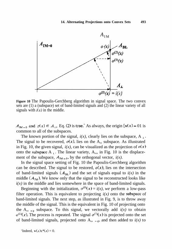
The geometry of the Papoulis-Gerchberg algorithm in a signal space isillustrated in Fig. 10. Shown is the subspace, Anr, consisting of allband-limited signals with a bandwidth not exceeding R. Also shown is thesubspace A,, = 0 consisting of all signals that are identically zero in theinterval 1x1 I X. Consider the set

A, = {U(X>lU(X) = 0, I.4 > XI.The subspace A I is orthogonal* to AIM-a because, for every w(x) E

*A i is said to be the orthogonal complement of AIMzO. Note that, if 9’,, projects ontoA,, =,, then 1 -9$, projects onto A i where 1 is an identity operator.


A I M

o(O)(x) = i(x)

Figure 10 The Papoulis-Gerchberg algorithm in signal space. The two convexsets are (1) a (subspace) set of band-limited signals and (2) the linear variety of allsignals with i(x) in the middle.

A,,=, and z(x) E A I , Eq. (2) is true.+ As always, the origin [U(X) = 01 iscommon to all of the subspaces.

The known portion of the signal, i(x), clearly lies on the subspace, A I .The signal to be recovered, o(x), lies on the A,, subspace. As illustratedin Fig. 10, the given signal, i(x), can be visualized as the projection of o(x)onto the subspace A I . The linear variety, A,,, in Fig. 10 is the displace-ment of the subspace, A,,=,, by the orthogonal vector, i(x).

In the signal space setting of Fig. 10 the Papoulis-Gerchberg algorithmcan be described. The signal to be restored, o(x), lies on the intersectionof band-limited signals (ABL) and the set of signals equal to i(x) in themiddle (AIM). We know only that the signal to be reconstructed looks likei(x) in the middle and lies somewhere in the space of band-limited signals.

Beginning with the initialization, o(‘)(x) = i(x), we perform a low-passfilter operation. This is equivalent to projecting i(x) onto the subspace ofband-limited signals. The next step, as illustrated in Fig. 9, is to throw awaythe middle of the signal. This is the equivalent in Fig. 10 of projecting ontothe A,, =. subspace. To this signal, we vectorally add i(x) to obtaino(l)(x). The process is repeated. The signal o(l)(x) is projected onto the setof band-limited signals, projected onto A,, = o, and then added to i(x) to

‘Indeed, w(x)z*(x) = 0.


form O(~)(X), etc. Clearly, the iteration is working its way along the set A,,toward the desired result, o(x).

The alternating projections in the Papoulis-Gerchberg algorithm areperformed between the subspace A,, and the linear variety A,,. Inspec-tion of Section 1V.A reveals the Papoulis-Gerchberg algorithm as aspecial case of Von Neumann’s alternating projection theorem.

C. HOWARD’S MINIMUM-NEGATMTY-CONSTRAINT ALGORITHM

Howard [34, 351 proposed a procedure for extrapolation of a interferomet-ric signal known in a specified interval when the spectrum of the signal wasknown (or desired) to be real and nonnegative. The technique was appliedto experimental inteferometric data and performs quite well.

As shown by Cheung et al. (361, Howard’s procedure was a special caseof POCS. Iteration is between the cone of signals with non-negativeFourier transforms defined by A,,, in Eq. (9) and the set of signals withidentical middles, A,, , as defined in Eq. (11). As with thePapoulis-Gerchberg algorithm, the middle is equal to the known portionof the signal.

The geometrical interpretation of Howard’s minimum-negativity-constraint algorithm is similar to that of the Papoulis-Gerchberg algo-rithm pictured in Fig. 10, except that the subspace A,, is replaced by acone corresponding to A,,,.

D. RESTORATION OF LINEAR DEGRADATION

In this section, POCS is applied to a linear degradation of a discrete timesignal. Denote the degradation operator by the matrix S and the degrada-tion by

i”= so’. (12)If the degradation matrix, S, is not full rank, a popular estimate of 0’ is thepseudo-inverse *

fsp, = [s%-&.

The projection matri.qt Ps, projects onto the column space of S.

Ps = s[sTs]-lsT (13)

*The solution, ZPI, is also referred to as the minimum norm solution.‘As is necessary for a projection operator, the projection matrix is idempotent: Pi = Ps.


AA

w-LD

II

-

II

d AD

I

OPIFigure 11 Illustration of restoration of a linear degradation. The signal to bereconstructed, 3, lies both on the linear variety A Is and on the convex set A,.

Consider the signal space illustrated in Fig. 11. The pseudo-inversesolution of Eq. (12) lies on the subspace A, onto which P, projects.Denote the orthogonal complement of A, by A I s. The projection opera-tor onto this space is simply

P I S = 1 - P,,

where 1 is an identity matrix. If the projection onto the orthogonalcomplement is

we are assured that

z=f3pI +o’, .

Define the linear variety

(14)

A LV = iilu'=i'+P,s~)t >

where u’ is any vector in the space.The pseudo-inverse solution can be improved using POCS if 0’ is also

known to satisfy one or more convex constraints. In other words


where {A,11 5 m i M} is the set of constraint sets and M is the numberof constraints. A set of corresponding projection operators can be defined:

{pm11 I m I Ml. (15)

In other words, gm projects an arbitrary signal onto A,.* Because thedesired solution, Z, is known to lie in each of the constraint sets, it followsthat

gmo’= o’, llmlM, (16)

and

o’=q&Y&i .*.p*.JY’,o’

=Y&, (17)

where

Tg ‘,YMYM-l ... .YD,L%dD,. (18)

Correspondingly, define the (nonempty) convex set

A, =A, nA,_, n ... nA, nA,,where n denotes intersection. Note that Yg does not project onto A,.As illustrated in Fig. 11, the desired signal to be reconstructed, o’, is knownto lie both in the convex set A, and the set A,,. A point in theintersection of these sets can be found using POCS. We have the POCSiteration

%N+i) =~L”~M%-* ‘..~az~J&)

‘~IJ~&‘V)

= T+ (I - Ps)~d.g~(N) (19)

The iteration is guaranteed to converge to a point on a solution set,

A solution = A, n ALV*

The solution will, in general, be nearer to 5 in the mean-square sense thanwas the pseudo-inverse. If Asolution consists of a single point, the solutionwill be unique.

The restoration in Eq. (19) is a generalization of (1) thePapoulis-Gerchberg algorithm for 9, =,~?a~ in Eq. (6) and (2) Howard’salgorithm for Td, =??ros in Eq. (10).

*When A, is a subspace, the projection operator is a matrix. That is, L?‘~ = P,.


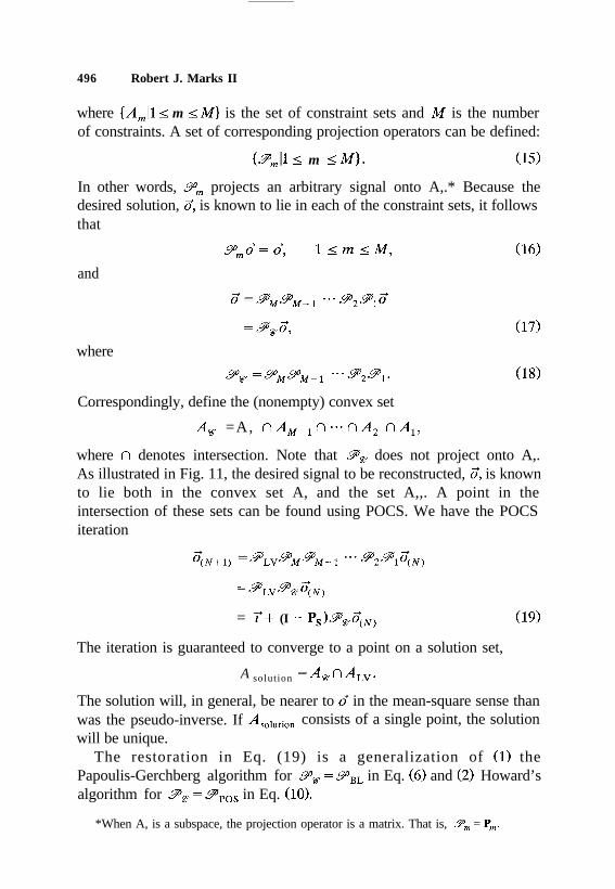
Figure 12 A geometrical example of slowly converging POCS. The intersection ofthe two linear varieties, far to the right, is the ultimate fixed point of the iteration.

V. Notes

In certain instances, POCS can converge painfully slowly. An example isshown in Fig. 12. One technique to accelerate convergence is relaxing theprojection operation by using a relaxed projection with parameter h [4]:

9relaxed = A9 + (I - /oz.

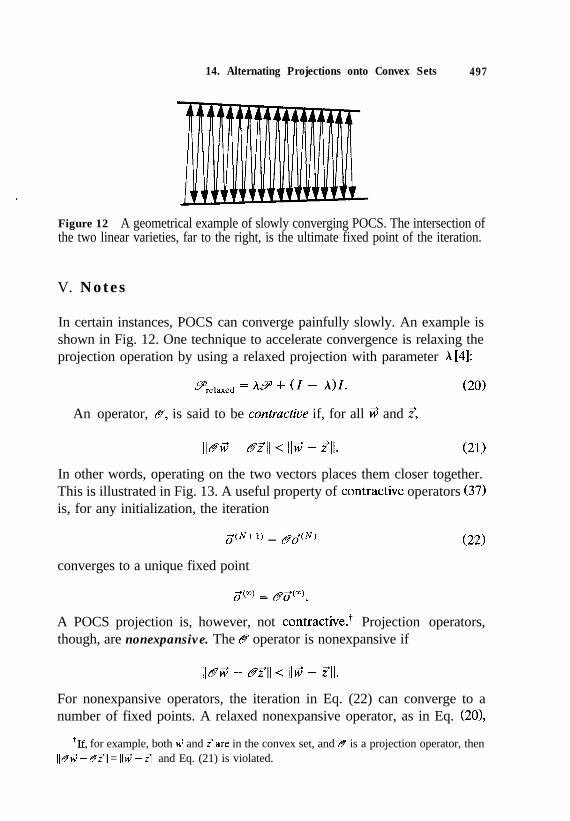
An operator, b, is said to be contra&e if, for all w’ and 2’,

(20)

Ilaw’ - myI < Ilw’ - z’ll. (21)

In other words, operating on the two vectors places them closer together.This is illustrated in Fig. 13. A useful property of contractive operators (37)is, for any initialization, the iteration

$N+i) = &?$W

converges to a unique fixed point

(221

$9 = @o”“‘.

A POCS projection is, however, not contractive.+ Projection operators,though, are nonexpansive. The B operator is nonexpansive if

Ilaw’ - &II 4 Ilw’ - z’ll.

For nonexpansive operators, the iteration in Eq. (22) can converge to anumber of fixed points. A relaxed nonexpansive operator, as in Eq. (201,

‘If, for example, both w’ and Zare in the convex set, and B is a projection operator, thenIl@w - 841 = Ilw’ - 31 and Eq. (21) is violated.


Figure 13 A geometrical example of slowly converging POCS. The intersection ofthe two linear varieties, far to the right, is the ultimate fixed point of the iteration.

however, is contractive (19). Applications of contractive operators do nothave the elegant geometrical interpretation of POCS.

VI. Conclusions

Restoration of degraded signals can, in many cases, be posed as a specialcase of alternating projection onto convex sets, or POCS. The object to berestored is known to lie in two or more convex constraint sets. Restorationcan be achieved by projecting alternately on each of the sets. If the setshave a nonempty intersection, then the projection will approach a fixedpoint lying in the intersection of the sets. If there are two sets that do notintersect, POCS will converge to a minimum mean-square error solution.If there are three or more sets with empty intersection, POCS yieldsresults that are not generally useful. Fuzzy POCS, however, can be used toobtain a result that is “close” to each of the constraint sets.

POCS is particularly useful in ill-posed deconvolution problems. Theproblem is regularized by imposing possibly nonlinear convex constraintson the solution set. Using the projection onto to the column space of theconvolution kernel as one of the constraints, POCS can be used, in manycases, to craft a desired result.


References

1. H. Stark, editor, “Image Recovery: Theory and Application.” Academic Press,Orlando, Florida, 1987.

2. L. M. Bregman, Finding the common point of convex sets by the method ofsuccessive projections. Dokl. Akud. Nauk. SSSR, 162 (No. 31, 487-490 (1965).

3. L. G. Gubin, B. T. Polyak, and E. V. Raik, The method of projections forfinding the common point if convex sets. USSR Comput. Math. Math. Phys.(Engl. Transl.) 7 (No. 61, l-24 (1967).

4. D. C. Youla and H. Webb, Image restoration by method of convex setprojections: Part I-Theory. IEEE Transactions on Medical Imaging MI-l,81-94 (1982).

5. M. I. Sezan and H. Stark, Image restoration by method of convex set projec-tions: Part II-Applications and Numerical Results. IEEE Transactions onMedical Imaging MI-l, 95-101 (1982).

6. S. J. Yen and H. Stark, Iterative and one-step reconstruction from nonuniformsamples by convex projections. J. Opt. Sot. Am. A 7, 491-499 (1990).

7. Hui Peng and H. Stark, Signal recovery with similarity constraints. J. Opt. Sot.Am. A 6 (No. 6), 844-851 (1989).

8. R. J. Marks II and D. K. Smith, Gerchberg-type linear deconvolution andextrapolation algorithms. In “Transformations in Optical Signal Processing”(W. T. Rhodes, J. R. Fienup, and B. E. A. Saleh, eds.), SPIE 373, pp. 161-178(1984).

9. M. Ibrahim Sezan, H. Stark, and Shu-Jen Yeh, Projection method formulationsof Hopfield-type associative memory neural networks. Appl. Opt. 29 (No. 17)2616-2622 (1990).

10. Shu-jeh Yeh and H. Stark, Learning in neural nets using projection methods.Optical Computing and Processing 1 (No. l), 47-59 (1991).

11. R. J. Marks II, A class of continuous level associative memory neural nets.Appl. Opt. 26, 2005-2009 (1987).

12. R. J. Marks II, S. Oh, and L. E. Atlas, Alternating projection neural networks.IEEE Trans. Circuits Syst. 36, 846-857 (1989).

13. S. Oh, R. J. Marks II, and D. Sarr, Homogeneous alternating projection neuralnetworks. Neurocomputing 3, 69-95 (1991).

14. R. J. Marks II, (ed.) “Advanced Topics in Shannon Sampling and InterpolationTheory.” Springer-Verlag, Berlin, 1993.

15. S. Oh, C. Ramon, M. G. Meyer, and R. J. Marks II, Resolution enhancementof biomagnetic images using the method of alternating projections. IEEETrans. Biomed. Ens. 40 (No. 41, 323-328 (1993).

16. S. Oh, R. J. Marks II, L. E. Atlas, and J. W. Pitton, Kernel synthesis forgeneralized time-frequency distributions using the method of projection ontoconvex sets. SPIE Proc. Znt. Sot. Opt. Eng. 1348, 197-207, (1990).


17. S. Oh, R. J. Marks II, and L. E. Atlas, Kernel synthesis for generalizedtime-frequency distributions using the method of alternating projections ontoconvex sets. IEEE Transactions on Signal Processing 42 (No. 71, 1653-1661(1994).

18. P. L. Combettes, The Foundation of Set Theoretic Estimation. Proc. IEEE 81,182-208 (19931.

19. M. H. Goldburg and R. J. Marks II, Signal synthesis in the presence of aninconsistent set of constraints. IEEE Trans. Circuits Syst. CAS-32 647-663(1985).

20. D. G. Luenberger, “Optimization by Vector Space Methods.” Wiley, NewYork, 1969.

21. D. C. Youla and V. Velasco, Extensions of a result on the synthesis of signalsin the presence of inconsistent constraints. IEEE Trans. Circuits Syst. CAS-33(No. 4), 465-468 (1986).

22.

23.

24.

25.

S. Oh and R. J. Marks II, Alternating projections onto fuzzy convex sets.Proceedings of the Second IEEE International Conference on Fuzzy Systems,(FUZZ-IEEE ‘93), San Francisco, March 1993 1, 148-155 (1993).R. J. Marks II, L. Laybourn, S. Lee, and S. Oh, Fuzzy and extra-crispalternating projection onto convex sets (POCS). Proceedings of the InternationalConference on Fuzzy Systems (FUZZ-IEEE), Yokohama, Japan, March, 20-24,1995, pp. 427-435 (1995).L. A. Zadeh, Fuzzy sets. Information and Control 8, 338-353 (1965); reprintedin J. C. Bezdek, (ed.) “Fuzzy Models for Pattern Recognition” IEEE Press,1992.J. Von Neumann, “The Geometry of Orthogonal Spaces.” Princeton Univ.Press, Princeton, New Jersey, 1950.

26.

27.

D. Slepian and H. 0. Pollak. Prolate spheroidal wave function Fourier analysisand uncertainty I. Bell Syst. Tech. J. 40, 43-63 (1961).R. J. Marks II, “Introduction to Shannon Sampling and Interpolation Theory.”Springer-Verlag, Berlin, 1991.

28. A. Papoulis, A new method of image restoration. Joint Services TechnicalActivity Report 39 (1973-1974).

29.

30.31.

32.

33.

A. Papoulis, A new algorithm in spectral analysis and bandlimited signalextrapolation. IEEE Trans. Circuits Syst. CAS-22, 735-742 (1975).A. Papoulis, “Signal Analysis.” McGraw-Hill, New York, 1977.R. W. Gerchberg, Super-resolution through error energy reduction. Opt. Acta21, 709-720 (1974).R. J. Marks II. “Introduction to Shannon Sampling and Interpolation Theory.”Springer-Verlag, Berlin, 1991.D. C. Youla, Generalized image restoration by method of alternating orthogo-nal projections. IEEE Trans. Circuits Syst. CAS-25, 694-702 (1978).


34. S. J. Howard, Fast algorithm for implementing the minimum-negativity con-straint for Fourier spectrum extrapolation. A@. Opt. 25, 1670-1675 (1986).

35. S. J. Howard, Continuation of discrete Fourier spectra using minimum-negativity constraint. J. Opt. Sot. Am. 71, 819-824 (1981).

36. K. F. Cheung, R. J. Marks II, and L. E. Atlas, Convergence of Howard’sminimum negativity constraint extrapolation algorithm. J. Opt. Sot. Am. A 5,2008-2009 (1988).

37. A. W. Naylor and G. R. Sell, “Linear Operator Theory in Engineering andScience.” Springer-Verlag, New York, 1982.

Deconvolutionof Images and Spectra

Second Edition

Edited by

Peter A. JanssonE. I. DU PONT DE NEMOURS AND COMPANY (INC.)

EXPERIMENTAL STATION

WILMINGTON, DELAWARE

0APACADEMIC PRESS

San Diego London BostonNew York Sydney Tokyo Toronto

Deconvolution of Images and Spectra - Robert...

Documents

Transcript of Deconvolution of Images and Spectra - Robert...