Decoding productivity:Business cycle properties of labor

productivity growth,by Arturo Estrella, FRB of NY

Presented and DiscussedBy Robert J. Gordon,

Northwestern University and NBER,CRIW Conference, July 27, 2004

The “Rainbow Connection”

• This is Arturo’s Powerpoint• This is Bob’s TITLE and text• Arturo’s Powerpoint is quite terse, so I’ve

expanded it quite a bit as part of the exposition– ANYTHING PURPLE IS DIRECTLY FROM

ARTURO’s PAPER

• The “New Economy” invades CRIW in technicolor!

Presenting vs. Discussing

• Two possibilities– #1, present first, discuss at end– #2, divide paper into blocks, discuss each in

sequence

• This paper deserves to be presented intact, discussion at end

• Insertions consist only of short previews of issues taken up later (watch the color!)

Overview

• Study behavior of labor productivity growth (BLS non-farm) at business cycle frequencies– (Note: no discussion of productivity trend, which is of

great interest to this audience, this is easily fixed)• Test hypotheses related to 3 issues from the

literature• Use frequency domain techniques, including

definition of business cycle– Important contribution of paper, contrast with time

domain that has previously dominated this literature– “only clear after decoding in frequency domain”

Issues

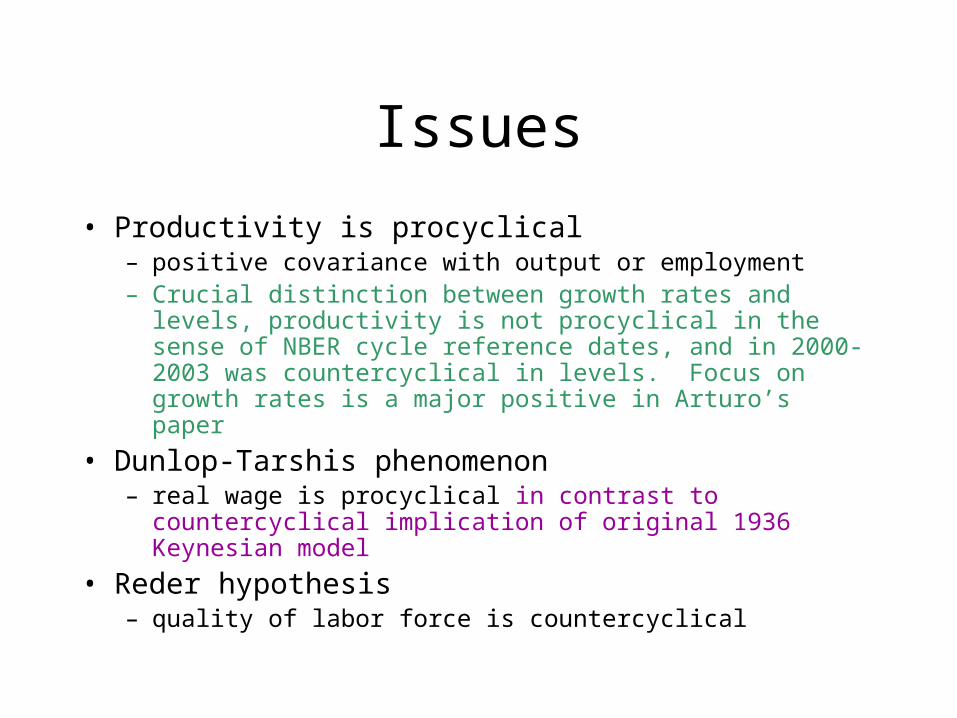
• Productivity is procyclical– positive covariance with output or employment– Crucial distinction between growth rates and levels, productivity is

not procyclical in the sense of NBER cycle reference dates, and in 2000-2003 was countercyclical in levels. Focus on growth rates is a major positive in Arturo’s paper

• Dunlop-Tarshis phenomenon– real wage is procyclical in contrast to countercyclical implication

of original 1936 Keynesian model

• Reder hypothesis– quality of labor force is countercyclical

Procyclical productivity

• Output and employment benchmarks• Output: Bernanke & Powell (1986), Gali (1999), Basu &

Fernald (2000)– All of these cites remark on the close positive correlation of

productivity GROWTH with output GROWTH, which is very different from the NBER cycle.

• Employment: Bernanke & Parkinson (1991), Christiano & Eichenbaum (1992), Basu (1996), Gali (1999)– This literature is about productivity vs. employment growth, not

different if employment and output growth are highly correlated.– Conventional literature doesn’t treat lags adequately as does

Arturo

Reasons for Procyclical Productivity

• Labor hoarding– Bernanke-Parkinson (1991) reject technology shocks,

adopt a combo of labor hoarding (variable labor utilization) and increasing returns to scale

– Basu (1996) mix of exogenous technology shocks and variable factor utilization.

– Basu-Fernald (2000) downplay tech shocks and emph variable factor utilz and resource reallocation.

• Oops, no cites to Oi, Okun, Hultgren (1960-62). Okun’s Law, Labor as a “quasi-fixed factor”

Why the y-n, n Correlation Should be Surprising

Covariances

cov( , )var( )yn

y nb

n

cov( , ) var( ) 1xn yn

c y n n n b

var( )cov( , ) var( )

var( )xy yn

yc y n y n b

n

Explanation of Equations

• The signs of the two covariances, y-n with n and y-n with y, are completely determined by the value of the regression coefficient byn.

• Productivity is procyclical with employment only if byn > 1

• Productivity is procyclical with output if byn < v (where v = var(y)/var(n)) which we should assume is > 1.Range of values 1 < byn < v for which both covars may be positive

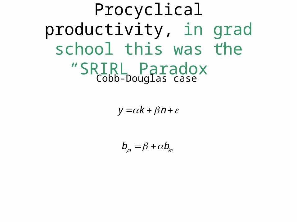
Procyclical productivity, in grad school this was the “SRIRL

Paradox” Cobb-Douglas case

y k n

yn knb b

Interpretation

• CRS, α+β = 1• byn = β + αbkn

– Assuming k,n positively correlated, that means estimator of β is upward biased, so that theoretical value of β < 1 is compatible with byn

> 1. (should distinguish between K stock and utilized K, link to Eichenbaum, Basu, etc.)

• If K and N used in fixed prop and CRS, then implied byn = 1 and cxn = 0 and cxy>1 if v>1

Hypotheses for Empirical Research

• x positively correlated with y?

• x positively correlated with n?

• y positively correlated with n?

• These questions will be addressed at the frequency domain so the crucial issue of leads and lags will be implicitly addressed

Dunlop-Tarshis

• Keynes (1936): real wage countercyclical– agreed with classics– labor demand curve– “. . . In general, an increase in the employment

can only occur to the accompaniment of a decline in the rate of real wages” (1936, p. 17)

Cyclical Productivity in theOriginal Keynesian Model

• Competitive factor pricing and Cobb-Douglas implication for labor’s share (S)

N

Y

P

W

N

Y

N

Y

NY

YN

PY

WNS

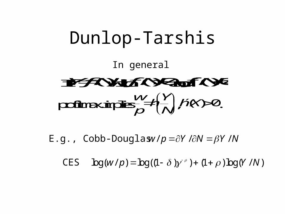
Dunlop-Tarshis

E.g., Cobb-Douglas

CES

/ / /w p Y N Y N

In general

If ()YfN with ()0fN and ()0fN ,

profit max. implies w Y

hp N

, ( ) 0hX .

log( / ) log((1 ) ) (1 ) log( / )w p Y N

Alternative with CES

• Real wage is a simple power function of productivity

• Relation is linear in logs and correlation is perfect• Further Hypotheses based on interpretation of

Keynes (1936) directly contradictory to #1, #2, and #3– #4: Δ(y-n) negatively correlated with Δy

– #5: Δ(y-n) negatively correlated with Δn

The Countercyclical Real Wage Hypothesis

• Dunlop (1938) and Tarshis (1939) found contrary evidence

• Preponderance of collected evidence still favours Dunlop-Tarshis– Abraham & Haltiwanger (1995) JEL review

• How can these guys cite macro from 1936 to 1939 without citing anything written from 1956 to 1981??– The “Missing Link” in American macro graduate

education!

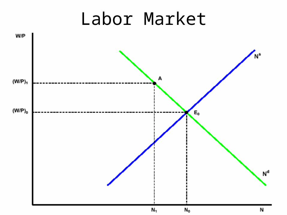
Labor Market

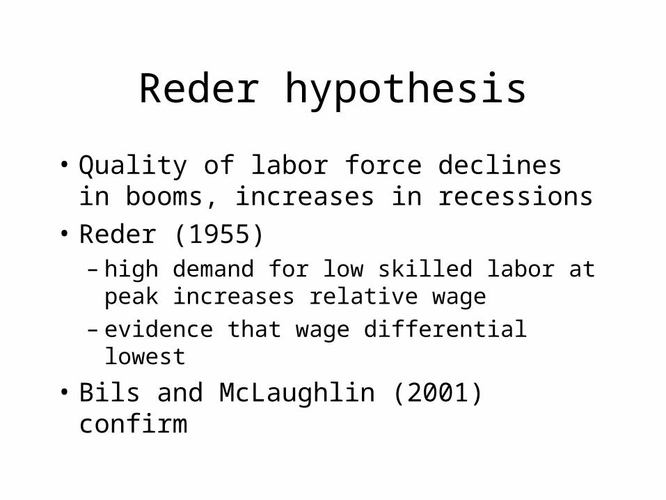
Reder hypothesis

• Quality of labor force declines in booms, increases in recessions

• Reder (1955)– high demand for low skilled labor at peak

increases relative wage– evidence that wage differential lowest

• Bils and McLaughlin (2001) confirm

Relation of Reder Hypothesis to Rest of Paper is Obscure

• First, problem, Reder hypothesis involves cyclical wage behavior across groups, but no relative wage data are included in paper

• McLaughlin and Bils (2001) find high wage industries have more cyclical employment and less cyclical wages.– No evidence in paper, could be unions, any

other source of wage rigidity. Let’s drop it, that’s another paper.

Suddenly the U Rate Appears

• Table 1 shows U a better predictor of NBER-defined recessions than either output or hours

• But the author forgets here the distinction between levels and rates of change. All the rest of the paper is about the rate of change of productivity, so the correlation between the LEVEL of U and the NBER dates is irrelevant.

Dropping into the Cauldron of Irrelevancy

• Hyp #6. Productivity is pos correlated with U rate

• Hyp #7. Productivity GROWTH is pos correlated with the U rate.

• Failure to relate U rate to basic economic variables y, n, y-n. Ignores the output identity that ties all these variables together.

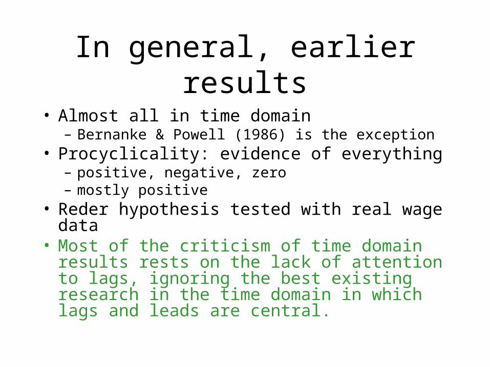
In general, earlier results

• Almost all in time domain– Bernanke & Powell (1986) is the exception

• Procyclicality: evidence of everything– positive, negative, zero– mostly positive

• Reder hypothesis tested with real wage data• Most of the criticism of time domain results rests

on the lack of attention to lags, ignoring the best existing research in the time domain in which lags and leads are central.

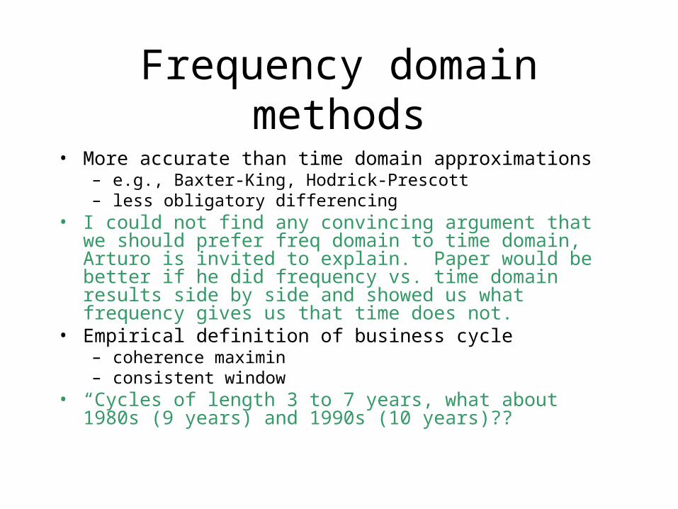
Frequency domain methods

• More accurate than time domain approximations– e.g., Baxter-King, Hodrick-Prescott– less obligatory differencing

• I could not find any convincing argument that we should prefer freq domain to time domain, Arturo is invited to explain. Paper would be better if he did frequency vs. time domain results side by side and showed us what frequency gives us that time does not.

• Empirical definition of business cycle– coherence maximin– consistent window

• “Cycles of length 3 to 7 years, what about 1980s (9 years) and 1990s (10 years)??

Frequency domain measures

• Reference frequency (-ies)• Coherence• In-phase correlation

– cf., dynamic correlation, Croux et al. (2001)

• In-phase regression– coefficient, R squared

• Phase lead• Sample period 1954:Q1 to 2003:Q1, similar to

Gordon (BPEA, 2003).

Productivity growth, low frequency and business cycle frequency components

Productivity Prod. growth

1954 1957 1960 1963 1966 1969 1972 1975 1978 1981 1984 1987 1990 1993 1996 1999 2002-7.5

-5.0

-2.5

0.0

2.5

5.0

7.5

10.0

12.5

15.0

Low freqs. Prod. growth

1954 1957 1960 1963 1966 1969 1972 1975 1978 1981 1984 1987 1990 1993 1996 1999 2002-7.5

-5.0

-2.5

0.0

2.5

5.0

7.5

10.0

12.5

15.0

The Paper’s Explanation of Figure 1

• The business cycle frequency (solid line) accounts for 9% of the variance of the series.

• The frequency domain analysis indicates correlations among variables at cyclical frequencies that automatically takes account of lags and leads (which has to be done consciously in time domain).

Alternative H-P trendsTTB and H-P methods

0.00

1.00

2.00

3.00

4.00

1955 1960 1965 1970 1975 1980 1985 1990 1995 2000

TTB

HP 1600

HP 6400

HP 25600

H-P 1,600

TTB

H-P 6,400

H-P 25,600

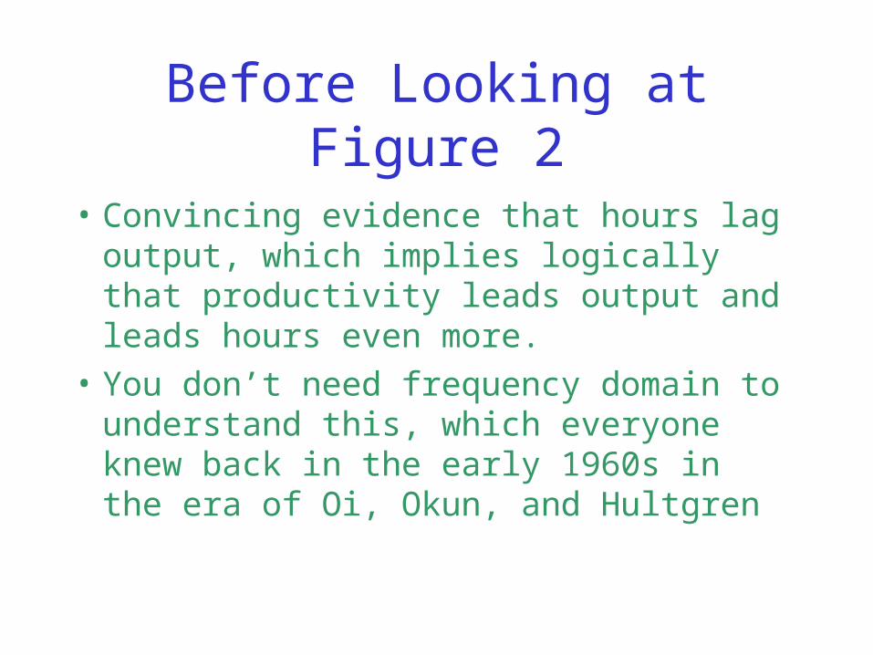
Before Looking at Figure 2

• Convincing evidence that hours lag output, which implies logically that productivity leads output and leads hours even more.

• You don’t need frequency domain to understand this, which everyone knew back in the early 1960s in the era of Oi, Okun, and Hultgren

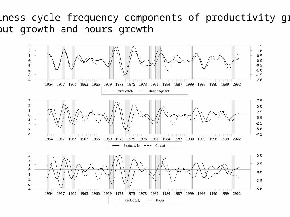
Business cycle frequency components of productivity growth,output growth and hours growth

Productivity Unemployment

1954 1957 1960 1963 1966 1969 1972 1975 1978 1981 1984 1987 1990 1993 1996 1999 2002-4-3-2-10123

-2.0-1.5-1.0-0.50.00.51.01.5

Productivity Output

1954 1957 1960 1963 1966 1969 1972 1975 1978 1981 1984 1987 1990 1993 1996 1999 2002-4-3-2-10123

-7.5

-5.0

-2.5

0.0

2.5

5.0

7.5

Productivity Hours

1954 1957 1960 1963 1966 1969 1972 1975 1978 1981 1984 1987 1990 1993 1996 1999 2002-4-3-2-10123

-5.0

-2.5

0.0

2.5

5.0

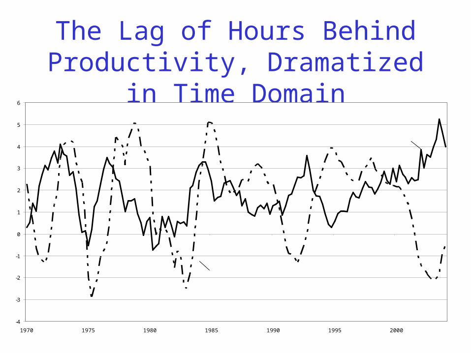
The Lag of Hours Behind Productivity, Dramatized in Time

Domain

-4

-3

-2

-1

0

1

2

3

4

5

6

1970 1975 1980 1985 1990 1995 2000

Productivity

Aggregate Hours

Table 2, Everything is Correlated with Everything

Look at all those high coherences, this says that everything is correlated with everything at the business cycle frequency in the frequency domain, which automatically allows for the obvious lags.

What about 2002-2003, really unusual, not mentioned in paper

Table 2. Coherences1954 Q1 to 2003 Q1

Var. 2Var. 1 x y n u

y .878(6.42)

-

n .839(5.71)

.972(9.99)

-

u .852(5.93)

.947(8.44)

.941(8.20)

-

u .848(5.86)

.960(9.15)

.977(10.48)

.946(8.39)

Table 3. In-phase correlation, proportion in-phase1954 Q1 to 2003 Q1

Var. 2Var. 1 x y n u

y .481(.300)

-

n .055(.004)

.902(.860)

-

u .805(.892)

.180(.036)

-.192(.042)

-

u -.044(.003)

-.876(.833)

-.977(.999)

.224(.056)

As We Would Expect, Zero In-phase Correlation of productivity with

hours• Look at next slide with results of Table 3

• Notice very small in-phase (contemporaneous) correlation of productivity with labor market variables

• Why is this interesting? Some naïve investigator could claim no positive, or even negative relation between y-n and n

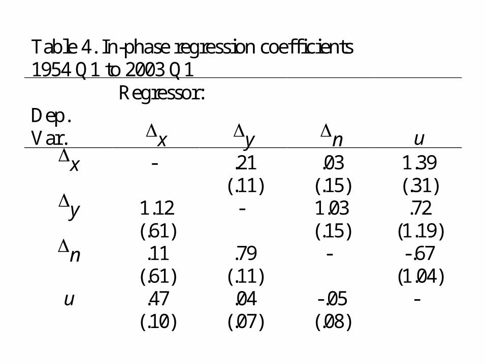
Table 4. In-phase regression coefficients1954 Q1 to 2003 Q1

Dep.Regressor:

Var. x y n ux - .21

(.11).03

(.15)1.39(.31)

y 1.12(.61)

- 1.03(.15)

.72(1.19)

n .11(.61)

.79(.11)

- -.67(1.04)

u .47(.10)

.04(.07)

-.05(.08)

-

Table 5. Phase: number of periods by which variable 1leads variable 21954 Q1 to 2003 Q1

Var. 2Var. 1 x y n u

y -2.60(.96)

-

n -3.95(1.14)

-1.01(.43)

-

u .88(1.08)

3.62(.60)

4.67(.63)

-

u 4.26(1.10)

7.14(.51)

8.17(.38)

3.50(.61)

Best Part of Empirical Results:Phase Leads and Lags

• Everything looks plausible and sensible – Lead of output ahead of hours– Lead of productivity ahead of output– (Double) lead of productivity ahead of hours

• Go back to my graph

The Lag of Hours Behind Productivity, Dramatized in Time

Domain

-4

-3

-2

-1

0

1

2

3

4

5

6

1970 1975 1980 1985 1990 1995 2000

Productivity

Aggregate Hours

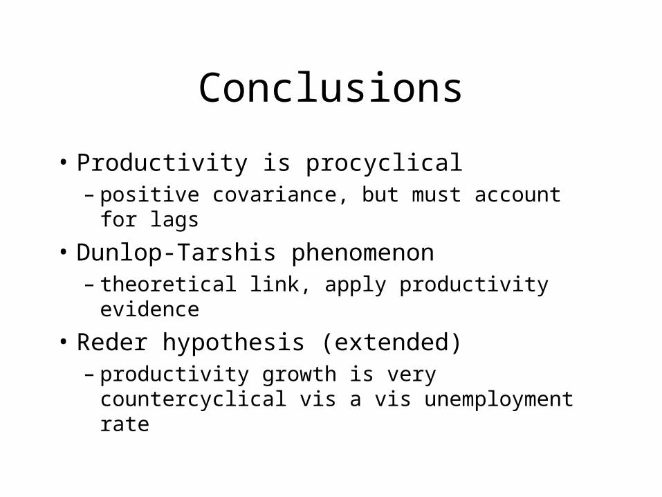
Conclusions

• Productivity is procyclical– positive covariance, but must account for lags

• Dunlop-Tarshis phenomenon– theoretical link, apply productivity evidence

• Reder hypothesis (extended)– productivity growth is very countercyclical vis

a vis unemployment rate

Discussion: Praise

• Cyclical Behavior of Productivity depends on getting the phase right

• Positive correlation of productivity with output is in RATES OF CHANGE not in LEVELS

• Phase discussion exactly right, productivity change leads output change leads hours change

• Not clear what frequency domain adds to ample evidence in time domain– Gordon (2003, Table 5) has Δn regressed on current

and lagged Δy AND Δ(y-n) regressed on LEADS of Δy

The “Output Identity” Organizational Tool for

Trends, Cycles, and Residuals

• The Output Identity• In its Simplest Form Makes Output (Q) Equal to the product of:

– Productivity (Q/A)– Hours per Employee (A/E)– Employment Rate (E/L), that’s just (1 – U/L)– Labor-force Participation Rate (L/N)– Working-age Population (N)

• Hiding Inside the Output Identity are Numerous Useful Trend and Cyclical Relationships, including

• OKUN’s Law. Recall the original 1962 breakdown. For every three percentage points of change in detrended output, 1 point for E/L, 1 point for productivity, ½ point for A/E, and ½ point for L/N.

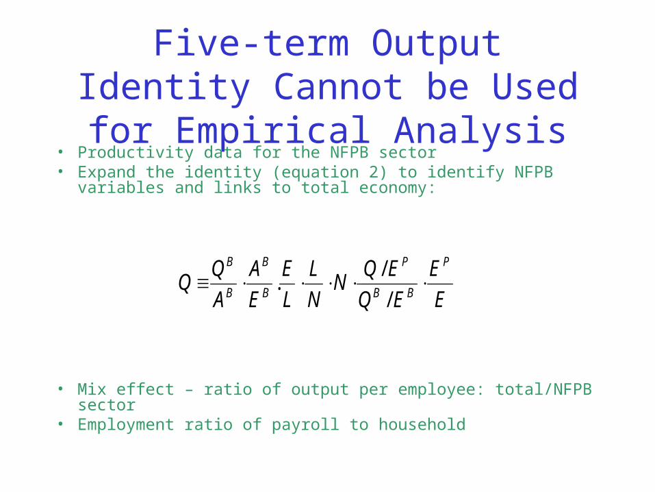
Five-term Output Identity Cannot be Used for Empirical Analysis

• Productivity data for the NFPB sector• Expand the identity (equation 2) to identify NFPB variables and links

to total economy:

• Mix effect – ratio of output per employee: total/NFPB sector• Employment ratio of payroll to household

E

E

EQ

EQN

N

L

L

E

E

A

A

QQ

P

BB

P

B

B

B

B

/

/.

Keynes, Dunlop, Tarshis, Arturo’s Astonish Literature Lapse

• Holy Grail, RJG “Output Fluctuations and Gradual Price Adjustment,” JEL, June 1981, pp. 502-03

• #1 Keynes rejected countercyclical interpretation in EJ March 1939– “. . . Short-period changes in real wages are usually so

small compared with the changes in other factors that we shall not often go far wrong if we treat real wages as substantially constant in the short period” (Keynes, 1939, pp. 42-43)

What is Left Out of Graduate Macro Education Today, but not in 1980?

• Non-market-clearing models

• Patinkin (1956, chapter 13)– Firms recognize a sales constraint on output at

a given level of W/P that forces them to operate off their classical Labor Demand curve

• The central non-market-clearing question. Are firms able to sell all they want at the market real wage? NO!!

Patinkin did the labor market, Clower did the expenditure market

• Clower coined the “effective demand curve” to describe firms which were unable to obtain their preferred combination of wage and employment in the labor market

• Patinkin (1956) and Clower (1965) were synthesized by Barro-Grossman (1971).

• The graph: why there is no presumption in Keynesian economics of a negative correlation between employment and the real wage

Labor Market 2

Going Beyond Paper, What About Labor’s Share?

• Assumed in false-Keynesian interpretation to be constant over the cycle

• A start at an interpretation

• Unique about price: partial adjustment to productivity

*

*/*

*/*

*/**

X

PW

NY

PWS

ZX

XPP )

*(*

)1(1 )*

(*)/*)(/(

*/

*

X

XZ

XXPP

WW

S

S

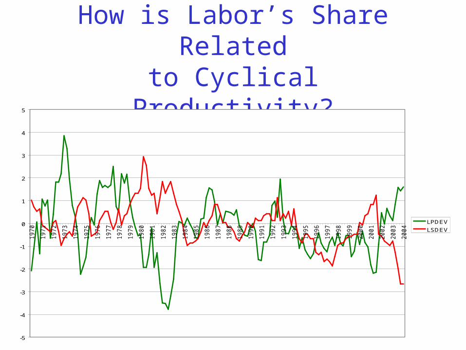
How is Labor’s Share Relatedto Cyclical Productivity?

-5

-4

-3

-2

-1

0

1

2

3

4

5

1970

1971

1972

1973

1974

1975

1976

1977

1978

1979

1980

1981

1982

1983

1984

1985

1986

1987

1988

1989

1990

1991

1992

1993

1994

1995

1996

1997

1998

1999

2000

2001

2002

2003

2004

LPDEV

LSDEV

Regression Results• ** drop lags• Linear Regression - Estimation by Least Squares• Dependent Variable C1LSHR• Quarterly Data From 1970:01 To 2004:01• Usable Observations 137 Degrees of Freedom 133• Centered R**2 0.264691 R Bar **2 0.248105• Uncentered R**2 0.264693 T x R**2 36.263• Mean of Dependent Variable 0.0007299270• Std Error of Dependent Variable 0.4330969784• Standard Error of Estimate 0.3755465201• Sum of Squared Residuals 18.757680107• Regression F(3,133) 15.9588• Significance Level of F 0.00000001• Durbin-Watson Statistic 2.072539

• Variable Coeff Std Error T-Stat Signif• *******************************************************************************• 1. Constant -0.000579057 0.032086045 -0.01805 0.98562839• 2. C1LPDEV -0.272623889 0.040989557 -6.65106 0.00000000• 3. CC1FAE 0.006115405 0.002978082 2.05347 0.04198668• 4. CC1RELIMP 0.013260474 0.004978166 2.66373 0.00868337

Conclusions

• Empirical analysis has it exactly right, study relation of changes to changes, not levels to levels

• Need to compare frequency to time domain to provide more convincing case of payoff to frequency domain

• Reder hypothesis can’t be tested without micro data

• Read Patinkin (1956) Chapter 13 and/or Barro-Grossman AER (1971). Keynesian model has NO implications for cyclical behavior of real wage or productivity