
DECLARATION - Latest News in Humanities and Social...
136
RELATIONSHIP BETWEEN ILLIQUIDITY AND STOCK RETURNS OF COMPANIES LISTED ATTHE NAIROBI SECURITIES EXCHANGE BY ARNOLD ADEM OKANGA D63/76511/2012 A RESEARCH PROJECT SUBMITTED IN PARTIAL FULFILMENT OF THE REQUIREMENT FOR THE AWARD OF THE DEGREE OF MASTER OF SCIENCE IN FINANCE, SCHOOL OF BUSINESS, UNIVERSITY OF NAIROBI 0
Transcript of DECLARATION - Latest News in Humanities and Social...
RELATIONSHIP BETWEEN ILLIQUIDITY AND STOCK
RETURNS OF COMPANIES LISTED ATTHE NAIROBI
SECURITIES EXCHANGE
BY
ARNOLD ADEM OKANGA
D63/76511/2012
A RESEARCH PROJECT SUBMITTED IN PARTIAL FULFILMENT
OF THE REQUIREMENT FOR THE AWARD OF THE DEGREE OF
MASTER OF SCIENCE IN FINANCE, SCHOOL OF BUSINESS,
UNIVERSITY OF NAIROBI
NOVEMBER 2014
0

DECLARATION
This research project is my original work and has not been submitted for the award of a
degree at the University of Nairobi or any other university.
Signature
ARNOLD A OKANGA
D63/76511/2012
Date
BY SUPERVISOR
This researchproject has been submitted for the examination with my approval as the
candidate’s Supervisor;
Signature
CYRUS IRAYA MWANGI
Supervisor
Department of Finance and Accounting
Date
ii

ACKNOWLEGEMENTS
I am grateful to the almighty God for giving me this opportunity to pursue Master of
Science degree in Finance degree at The University of Nairobi.
I thank my supervisor, Cyrus IrayaMwangi whose guidance and support enabled me
to complete this research.
I acknowledge all previous works that I have cited in this research document, for the
enlightenment they gave me, and the methodological approach to the research they
conducted.
iii

DEDICATION
To my family for their continued support in my life’s pursuits, to the University of
Nairobi, The University of Witwatersrand Johannesburg, St. Johns Emerald Hill Harare,
Allan Wilson Boys High School Harare and Sony Sugar Primary School for molding me
to whom I am to date. I would like to make a special dedication to my wife Joan Oracha
for her strategic objective view of life and her influence to the pursuit of my goals, thank
you for being the rock in my life. To my father, Mr. O.C. Okanga, who always has faith
in my abilities and all my accomplishments, thank you for always being around and
ensuring that my abilities are realised. And a special thanks to my mother, Mrs G. A.
Okanga, who always preached of living me to my vices for an educated out come and
independent thoughts.
iv

TABLE OF CONTENTS
DECLARATION.................................................................................................................ii
ACKNOWLEGEMENTS..................................................................................................iii
DEDICATION....................................................................................................................iv
TABLE OF CONTENTS.....................................................................................................v
LIST OF TABLES..............................................................................................................ix
ABBREVIATIONS...........................................................................................................xii
ABSTRACT.....................................................................................................................xiii
CHAPTER ONE: INTRODUCTION..................................................................................1
1.1 Background of the Study...................................................................................1
1.1.1 Stock Illiquidity.................................................................................................2
1.1.2 Stock Returns.....................................................................................................4
1.1.3 Relationship between Illiquidity and Stock Returns.........................................5
1.1.4 Nairobi Securities Exchange..............................................................................6
1.2 Research Problem..............................................................................................7
1.3 Research Objective............................................................................................8
1.4 Value of this Study............................................................................................9
CHAPTER TWO: LITERATURE REVIEW....................................................................10
v

2.1 Introduction......................................................................................................10
2.2 Theoretical Review..........................................................................................10
2.2.1 The Bid-Ask Spread Theory............................................................................10
2.2.2 The Classic Stock Pricing Theory...................................................................11
2.2.3 The Capital Asset Pricing Theory....................................................................11
2.2.4 Arbitrage Pricing Theory.................................................................................12
2.2.5 The Clientele Effect.........................................................................................12
2.2.6 The Trading Volume Theory...........................................................................13
2.3 Determinant of Stock Returns.........................................................................13
2.3.1 Risk Free Rate..................................................................................................14
2.3.2 Market Return..................................................................................................14
2.3.3 Risk Premium..................................................................................................14
2.3.4 Illiquidity.........................................................................................................15
2.4 Review of Empirical Studies...........................................................................15
2.5 Summary of Literature Review.......................................................................21
CHAPTER THREE: RESEARCH METHODOLOGY....................................................22
3.1 Introduction......................................................................................................22
3.2 Research Design..............................................................................................22
3.3 Population of Study.........................................................................................22
vi

3.4 Sample and Sampling Design..........................................................................23
3.5 Data Collection Techniques.............................................................................23
3.6 Data Analysis...................................................................................................24
3.6.1 Illiquidity Calculations....................................................................................24
3.6.2 Determining Relationship between Illiquidity and Stock Returns..................25
3.7 Test of Significance.........................................................................................26
CHAPTER FOUR: DATA ANALYSIS, RESULTS AND DISCUSSION......................27
4.1 Introduction......................................................................................................27
4.2 Portfolio Formation Process............................................................................27
4.3 Descriptive Statistics.......................................................................................28
4.4 Illiquidity Measure...........................................................................................28
4.2.1 First Liquidity Proxy: Return to Volume Ratio...............................................29
4.2.2 Second Liquidity Proxy: Reversal Measure of Illiquidity...............................29
4.5 Beta Estimation Process..................................................................................30
4.6 Cross-sectional Testing Process......................................................................30
4.7 Interpretation of Findings................................................................................38
CHAPTER FIVE: SUMMARY, CONCLUSION AND RECOMMENDATIONS.........40
5.1 Introduction......................................................................................................40
5.2 Summary of Findings......................................................................................40
vii

5.3 Conclusion.......................................................................................................41
5.4 Recommendations............................................................................................42
5.5 Limitation of Study..........................................................................................43
5.6 Suggestion for Further Research.....................................................................43
REFERENCES..................................................................................................................45
APPENDICES...................................................................................................................50
APPENDIX I: List of Stocks at the NSE as at December 2013........................................50
APPENDIX II: Portfolio formation...................................................................................54
APPENDIX III: Cross-sectional testing results under 2nd ILLQ measure.........................64
viii

LIST OF TABLES
Table 4.1a: Descriptive Statistic on deals, volume and turnover 28
Table 4.1b: Descriptive Statistic on deals, volume and turnover 28
Table 4.2: Calculated Illiquidity x10^-9 for portfolios, 1st Illiquidity Measure 29
Table 4.3: Calculated Illiquidity x10^-9 for portfolios, 2nd Illiquidity Measure 29
Table 4.4: Calculated Beta for portfolios under study 30
Table 4.5: Summary output of Cross-sectional testing under 1st ILLQ measure 31
Table 4.6 a: ANOVA of Cross-sectional testing under 1st ILLQ measure, P1 to P15..32
Table 4.6 b: ANOVA of Cross-sectional testing under 1st ILLQ measure, P16 to P30..33
Table 4.7 a: Result of Coefficients, for Cross-sectional testing under 1st ILLQ measure,
P1 to P10 34
Table 4.7 b: Result of Coefficients, for Cross-sectional testing under 1st ILLQ measure,
P11 to P20 35
Table 4.7 c: Result of Coefficients, for Cross-sectional testing under 1st ILLQ measure,
P21 to P30 36
Table A.1: P1, Portfolio of Largest Size (Deals) at Jan 2009 54
Table A.2: P2, Portfolio of Smallest Size (Deals) at Jan 2009 54
Table A.3: P3, Portfolio of Largest Volume at Jan 2009 54
Table A.4: P4, Portfolio of Smallest Volume at Jan 2009 55
ix

Table A.5: P5, Portfolio of Largest Turnover at Jan 2009 55
Table A.6: P6, Portfolio of Smallest Turnover at Jan 2009 55
Table A.7: P7, Portfolio of Largest Size (Deals) at Jan 2010 56
Table A.8: P8, Portfolio of Smallest Size (Deals) at Jan 2010 56
Table A.9: P9, Portfolio of Largest Volume at Jan 2010 56
Table A.10: P10, Portfolio of Smallest Volume at Jan 2010 57
Table A.11: P11, Portfolio of Largest Turnover at Jan 2010 57
Table A.12: P12, Portfolio of Smallest Turnover at Jan 2010 57
Table A.13: P13, Portfolio of Largest Size (Deals) at Jan 2011 58
Table A.14: P14, Portfolio of Smallest Size (Deals) at Jan 2011 58
Table A.15: P15, Portfolio of Largest Volume at Jan 2011 58
Table A.16: P16, Portfolio of Smallest Volume at Jan 2011 59
Table A.17: P17, Portfolio of Largest Turnover at Jan 2011 59
Table A.18: P18, Portfolio of Smallest Turnover at Jan 2011 59
Table A.19: P19, Portfolio of Largest Size (Deals) at Jan 2012 60
Table A.20: P20, Portfolio of Smallest Size (Deals) at Jan 2012 60
Table A.21: P21, Portfolio of Largest Volume at Jan 2012 60
Table A.22: P22, Portfolio of Smallest Volume at Jan 2012 61
Table A.23: P23, Portfolio of Largest Turnover at Jan 2012 61
x
Table A.24: P24, Portfolio of Smallest Turnover at Jan 2012 61
Table A.25: P25, Portfolio of Largest Size (Deals) at Jan 2013 62
Table A.26: P26, Portfolio of Smallest Size (Deals) at Jan 2013 62
Table A.27: P27, Portfolio of Largest Volume at Jan 2013 62
Table A.28: P28, Portfolio of Smallest Volume at Jan 2013 63
Table A.29: P29, Portfolio of Largest Turnover at Jan 2013 63
Table A.30: P30, Portfolio of Smallest Turnover at Jan 2013 63
Table A31: Summary output of Cross-sectional testing under 2nd ILLQ measure 64
Table A32 a: ANOVA of Cross-sectional testing under 2nd ILLQ measure, P1 to P15..65
Table A32 b: ANOVA of Cross-sectional testing under 2nd ILLQ measure, P16 to P30..66
Table A33 a: Result of Coefficients, for Cross-sectional testing under 2nd ILLQ measure,
P1 to P10 67
Table A33 b: Result of Coefficients, for Cross-sectional testing under 2nd ILLQ measure,
P11 to P20 68
Table A33 c: Result of Coefficients, for Cross-sectional testing under 2nd ILLQ measure,
P21 to P30 69
xi

ABBREVIATIONS
AMEX – American Stock Exchange
APT – ArbitragePricing Theory
ATS - Automated Trading Systems
CAPM – CapitalAsset Pricing Model
CMA - Capital Markets Authority
DASS - Delivery and Settlement System
FISD - Financial Information Services Division
HPY - Holding Periods Yield
ILLIQ - Illiquidity Measure
LIQ- Liquidity Measure
LVW - Lori Van Dusen
NSE - Nairobi Securities Exchange formally Nairobi Stock Exchange
NYSE - New York Stock Exchange
OLS - Ordinary Least Square
OTC - Over the Counter Markets
SIIA - Software and Information Industry Association
US$ - United States Dollar/s
xii

ABSTRACT
The objective of this study was to determine the relationship between illiquidity and stock returns of companies listed at the Nairobi Securities Exchange. The research design was descriptive using two proxies to Illiquidity, the return to volume ratio which was proposed by Amihud (2002) and reversal measure of illiquidity advocated by Pastor and Stambaugh (2003), in a cross-sectional framework of Fama and Macbeth (1973), the study was undertaken to ascertain the nature of this relationship at the NSE for a5 year period 2009- 2013.The data was obtained from the Nairobi Securities exchange in a daily format, which was then converted to a monthly format to fit with the research design, the Sample comprised of portfolios created from stocks that were continuously traded during this period. The Illiquid test carried out using the two proxies to illiquidity showed significantly high Illiquidity for portfolios that had stocks whose characteristics had either fewer deals at the exchange, lowest volume, or lowest turnover respectively. Portfolio of stocks which bore high trade deals, high volume and highest turnover had low illiquidity.Illiquidity portfolio return relationship was established using the three variables, volume, illiquidity and market premium. Test of the Fama and Macbeth (1973) models significance, F-test, revealed a p-value well below 0.5% for a 99% confidence interval, showing strong significance level for all the 30 portfolios. This was an indicator that illiquidity positively affects stock returns at the Nairobi Securities Exchange, a relationship such that higher illiquidity would translate to above the market returns. This is consistent with major study findings that, since illiquidity is persistent, illiquidity predicts future returns and illiquidity co-moves with contemporaneous returns, this is as positive shock to illiquidity predicts high future illiquidity
xiii
CHAPTER ONE: INTRODUCTION
1.1 Background of the Study
The nature of stock illiquidity or liquidity thereof has prompted vast amount of research
and is still a challenging issue in finance, due to the many facets of liquidity. Literature
on liquidity as a systematic risk factor that can help explain the nature of stock returns
has evolved in the recent years with major studies focused on the developed markets were
the issue was first recognized as a contributing factor to stock returns: Amihud and
Mendelson (1986); Datar, Naik, and Radcliffe (1998), just to mention a few.
Kim, Farmer and Lo (2007) identified two facets of liquidity: execution time and
probability of execution of limit orders; and price impact of market orders. Amihud,
Mandelson and Perdesen (2005)argue that, liquidity has many facets, and that a major
problem in estimating the effect of liquidity on asset returns is how to measure liquidity
since there is hardly any single measures used that captures all its aspects.
How returns at the Nairobi Security Exchange fairs on with its current illiquidity, and
liquidity conditions in meeting different stock investor objectives, in line with similar
investor objectives in well establish exchanges becomes of interest to most equity
analysts and investors, and is a motivating factor that has lead to this study. Note that in
this study Liquidity and Illiquidity will be used interchangeably but with specific
reference, since both measure the same factor but from different ends of liquidity-
illiquidity spectrum.
1
1.1.1 Stock Illiquidity
Liquidity refers to the ease by which an asset can be sold immediately after purchase
without lowering the price and without incurring transaction cost (Dalgaard, 2009).
Liquidity is a broad and elusive concept that generally denotes the ability to trade large
quantities quickly, at low cost, and without moving the price (Pastor and Stambaugh,
2003). Illiquidity is the converse of liquidity as per the definitions above, and the main
source of illiquidity normally are:exogenous transaction costs, which include brokerage
fees, stocks buy or sell order processing cost, transaction taxes and the likes;Demand
pressure and inventory risk, which is caused by the availability of buying and selling
agents on demand;Information Asymmetry or Private information, these are material
information about the fundamentals of a company or order flow;Search friction, these are
opportunity costs linked to the difficulty of locating a counterparty, this is particularly
relevant in the over the counter (OTC) markets(Amihud et al, 2005).Illiquidity in this
context refers to the degree of friction in a given exchange market, where there is a
measurable extent of cost of exchange, agents price distortion and movements.
Illiquidity has wide ranging effects on financial markets,in a look at its converse,
liquidity can explain cross-section of assets with different liquidity, after controlling for
other assets characteristics such as risk, and time series relationship between liquidity and
security return. Liquidity explains why certain hard-to-trade securities are relatively
cheap, the pricing of stock and corporate bonds, the return on hedge funds, and the
valuation of closed-end funds. It follows that liquidity can help explain a number of
2

puzzles, such as why equities commanding high required returns (the equity premium
puzzle), why liquid risk-free treasuries have low required returns (the risk-free rate
puzzle), and why small stocks that are typically illiquid earn high returns (the small firm
effect) (Amihud et al, 2005).
Illiquidity can be measure by measuring the sources of elements of illiquidity,as
mentioned above, the Exogenous Transaction Costs, Demand Pressure and Inventory
risk, Information Asymmetry or Private information, Search friction. Noting
thatspecifically the cost of illiquidity can be measured in the following ways: Trading
volume, which measures volumes, traded in a given day. Its advantage is that it is simple
and available. It’s down side is in the volumes-volatility relation, as volatility can impede
market liquidity; Trading frequency, which measures the number of trades executed
within a specific interval, without regards to size. But it too can be associated with; using
the bid – ask spread, which is the difference between bid price (stocks sales price) and
ask price (stocks purchase price), measures the cost of executing a small trade; Quote
size, which is the quantity of securities tradable at the bid and offer prices, it accounts for
the market depth and complements the bid-ask spread; Trade size, which is the quantities
of securities traded at bid and offer prices, reflecting any negotiation over quantity. It’s an
alternative depth measure; Price impact coefficient,considers the rise and fall in prices
that typically occurs with a buyer initiated or a seller initiated trade (Pastor and
Stambaugh, 2003).
3

1.1.2 Stock Returns
Investors invest to earn returns from savings due to their differed consumption (Reilly
and Brown, 2012). One can then deduce from this that a return is a compensation an
investor receives for the period of investment in which they are exposed to expected
inflation and uncertainty of future cash flow. Stock returns are the returns that the
investors generate out of the stock market either in the form of profits through trading or
from dividends given by the company to its shareholders from time to time. Stock returns
are not fixed ensured returns, and are subjected to market risk, they are not homogeneous
and may change from investor to investor depending on the amount of risk one is
prepared to take and the quality of his stock market analysis.
Most investors require higher rates of return on investment if they perceive there is any
uncertainty about the expected rate of return. This increase in the required rate of return
over the nominal risk-free rate is the risk premium. Most prominent sources of this
uncertainty are: business risk; financial risk (leverage); liquidity risk; exchange rate risk
and country (political) risk (Reilly and Brown, 2012). The uncertainty of how fast an
investment can be bought or sold,or the existence of uncertainty about its price, increases
liquidity risk. Liquidity risk can be a significant consideration when investing in foreign
securities depending on the country and the liquidity of its stock and bond markets
(Reilly and Brown, 2012).
Returns are measured in two ways, the historical rate of return and the expected rate of
return, this paper depends on the use of the first measure. The historical rate of return is
the return on an investment over the time period the investment is held (the holding
4

period) (Reilly and Brown, 2012). The holding period return as a percentage term in
annual basis and is a measure referred to as the holding periods yield (HPY). For a
portfolio of investment, the mean historical rate of return (HPY) for a portfolio of
investments is measured as the average of the HPYs for the individual investmentsin the
portfolio
1.1.3 Relationship betweenIlliquidity and Stock Returns
If Illiquidity affects asset prices, it stands that changes in liquidity should change asset
prices (ceteris paribus). This hypothesis was examined by Amihud et al. (1990). Liquidity
asset pricing theory implies that, a downward revision in liquidity should cause a decline
in stock price. Further, theoretically expected returns are an increasing function of
illiquidity cost, and that their relationship is concave due to the clientele effect.
Empirically, studies that investigate the relationship between Illiquidity/liquidity and
asset prices include Amihud and Mendelson (1986), Brennan and Subrahmanyan (1996),
Datar, Naik, and Radcliffe (1998), Brennan, Chordia, and Subrahmanyan (1998), Fiori
(2000), Chan and Faff (2005), Acharya and Pedersen (2005), among others using a
variety of liquidity measures, these studies generally find that less liquid stocks have a
higher average returns (Pastor and Stambaugh, 2003). Chordia et al. (2001) found a
significance cross-sectional relation between stock returns and the variability of liquidity
(Pastor and Stambaugh, 2003).In Kenya Njiinu (2007) found significant changes in
liquidity in the NSE for the period under study, Gacheru (2007)findings revealed that,
there was no significant association between the trading volume and security market
5

prices at the NSE. Koech (2012)concluded that there was a non-liner relationship
between liquidity and returns of listed firms in the NSE.
1.1.4 Nairobi Securities Exchange
In 1951, an Estate Agent by the name of Francis Drummond established the first
professional stock broking firm. In 1954 the Nairobi Stock Exchange was then
constituted as a voluntary association of stockbrokers registered under the Societies Act.
In July 1994 a computerized delivery and settlement system (DASS) came into effect. In
September 2006 live trading on the automated trading systems (ATS) of the Nairobi
Stock Exchange was implementedtrading hours increased to three hours (10:00 am – 1:00
pm). In February 2007 NSE upgraded its website to enhance easy and faster access of
accurate, factual and timely trading information. In July 2011, the Nairobi Stock
Exchange Limited changed its name to the Nairobi Securities Exchange Limited. The
change of name reflected the strategic plan of the Nairobi Securities Exchange to evolve
into a full service securities exchange which supports trading, clearing and settlement of
equities, debt, derivatives and other associated instruments. In March 2012, the Nairobi
Securities Exchange became a member of the Financial Information Services Division
(FISD) of the Software and Information Industry Association (SIIA). (2014, July 15)
https://www.nse.co.ke/about-nse/history-of-organisation.html
The Nairobi Securities Exchange is licensed and regulated by the Capital Markets
Authority (CMA). It has the mandate of providing a trading platform for listed securities
and overseeing its Member Firms.The Capital Markets Authority is the Government
Regulator charged with licensing and regulating the capital markets in Kenya. It also
6

approves public offers and listings of securities traded at the Nairobi Securities
Exchange.The Central Depository and Settlement Corporation provides clearing, delivery
and settlement services for securities traded at the Nairobi Stock Exchange. It oversees
the conduct of Central Depository Agents comprised of stockbrokers and investments
banks which are members of NSE and Custodians. Nairobi Security exchange (2014, July
15) https://www.nse.co.ke/regulatory-framework.html
The volume traded in the NSE has increased as at the 20 th January 2012, volume of US$
1,164,034 was traded and at the 6th July 2013, a volume of US$ 4,323,391 was traded a
271% change(LVW advisors. Aug 2013)
Studies of stock returns at the NSE has had a mix and enriching information source,
including the following: There was no significant association between trading volume
and security market prices at the NSE, this study however indicated that large
capitalization portfolio of securities exhibited high price-to-volume correlation as
opposed to small capitalization portfolio of stocks (Gacheru, 2007); Volatility of stocks
return in Kenya listed companies’ increase around general elections (Lusinde, 2012); the
returns of companies quoted at the NSE are determined byfactors other than size and ratio
of book to market value (Oliech, 2002); there is a non-liner relationship between liquidity
and the returns of listed firms at the Nairobi Securities Exchange (Koech, 2012).
1.2 Research Problem
A security’s required return depends on its expected liquidity as well as on the
covariances of its own return and liquidity with the market return and liquidity. In
addition, a persistent negative shock to a security’s liquidity results in low
7
contemporaneous returns and high predicted future returns (Acharya and Pedersen,
2005). Studies as to whether expected returns are related to the level of liquidity reveal
that illiquid stocks have higher average returns.
As noted in the last section research on NSE illiquidity/liquidity has had a mix of results,
from works that find no significant association between trading volume and security
market prices at the NSE, while at the same time security prices of high price to volume
correlation for large capitalization as opposed to small capitalization portfolios (Njiinu,
2007).
Further in the Kenyan context, Songole (2012) studied the relationship between selected
macroeconomic variables and stock return in the NSE, Lusinde (2012) in his paper
volatility in stock returns of NSE listed companies around general elections in Kenya
studied the cyclic behavior of stock returns around election period, Koech(2012) in his
paper looked at the relationship between Liquidity and return of stocks at the Nairobi
securities exchange, based on the correlation of 57 listed firms in the NSE, during the
period between 2007 to 2011, using turnover rate as a proxy to liquidity, Wanjiru (2013)
in his paper looked at the relationship between liquidity and cross listing of shares cross
listed in the East Africa Security exchanges. This study seeks to ascertain the following
questions:Is liquidity incorporated on stock prices at the NSE? And if so, is the
relationship between liquidity and stock returns at the NSE convex?
1.3 Research Objective
Todetermining the relationship between illiquidity and stock returns of companies listed
at the Nairobi Securities Exchange.
8

1.4 Value of this Study
To the world of finance, this study will extend and apply the knowledge of the
relationship between liquidity and returns by testing this relationship in the Nairobi
securities exchange. The findings are expected to further contribute to the understanding
of frontier market liquidity and aid in investment strategies that relate to the Nairobi
Securities Exchange.
To the Nairobi Securities Exchange, this study will enhance the understanding of
liquidity of companies listed at the exchange, increasing the knowledge of the nature of
the exchange to current and potential investors.
To portfolio managers, the study will enhance the understanding of the liquidity nature of
stocks at the Nairobi Securities Exchange, improving on their investment strategies with
the aim of outperforming the returns of Nairobi Securities Exchange related benchmarks.
To foreign investors, this study will provide the much needed information on the liquidity
of stocks at the Nairobi Securities Exchange,in relation to including or extending their
portfolio exposure to include NSE stocks for diversification purposes.
9

CHAPTER TWO: LITERATURE REVIEW
2.1 Introduction
Thischapter highlights major theories and seeks to evaluate previous studies in relation to
Illiquidity or liquidity and asset returns:Section 2.2Presents theoretical review of liquidity
and asset returns; Sections 2.3Presents determinants of stock returns; Section 2.4Presents
a review of selected major studies on liquidity in relation to asset returns and ends with
review oflocal studies that have captured aspects of liquidity, asset returns or both.The
review presents objective, methodology findings and implications of these
studies;Section 2.5 Containsa summary of the literature review.
2.2 Theoretical Review
Studies of Market Microstructure have looked at the processes and outcome of
exchanging assets under explicit trading rules, such studies test the Efficient Market
Hypothesis. Some important theories that relate stock return to liquidity are: The Bid-ask
spread theory; The Classic Stock Pricing Theory; The Capital Asset Pricing Theory;
Arbitrage Pricing Theory;The Clientele Effect; and The Trading Volume Theory to
mention a few.
2.2.1 The Bid-Ask Spread Theory
Bid-ask spread theory by Thomas, Copeland and Galai (1983), theories that an individual
who chooses to serve as a market-maker is assumed to optimize his position by setting a
bid-ask spread which maximizes the difference between expected revenues received from
10

liquidity-motivated traders and expected losses to information-motivated traders. By
characterizing the cost of supplying quotes, as writing a put and a call option to an
information-motivated trader, it is shown that the bid-ask spread is a positive function of
the price level and return variance, a negative function of measures of market activity,
depth, and continuity, and negatively correlated with the degree of competition.
2.2.2 The Classic Stock Pricing Theory
The classic stock pricing theory states that the basic Idea behind the dividend based stock
valuation is that the value of a stock is the present value of all future dividends (Williams,
1938). In the financial markets therefore, the maximum price that investors are willing to
pay for a financial asset is actually the current value of future cash payments that are
discounted at a higher rate to compensate for the uncertainty in the cash flow projections.
2.2.3 The Capital Asset Pricing Theory
The Capital Asset Pricing Model (CAPM) was introduced by Treynor (1961, 1962),
Sharpe (1964), Lintner (1965) and Mossin (1966) independently building on the work of
Markowits. Itpostulates that the variation in stock returns is solely determined by the
market beta. (CAPM) for general equilibrium relationship in capital markets captures the
return of an asset as directly equal to the risk free rate and market risk factor, beta,
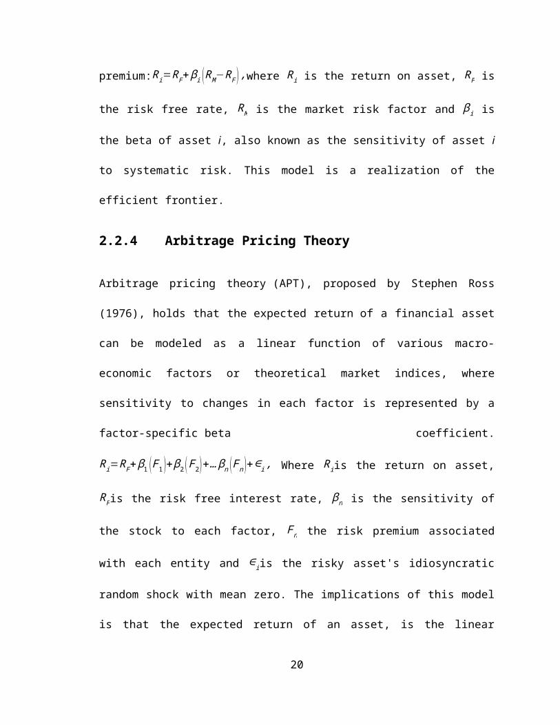
multiplied by the risk premium:Ri=RF+ βi ( RM−RF ) ,where Ri is the return on asset, RF is
the risk free rate, RM is the market risk factor and β i is the beta of asset i, also known as
the sensitivity of asset i to systematic risk. This model is a realization of the efficient
frontier.
11

2.2.4 Arbitrage Pricing Theory
Arbitrage pricing theory (APT), proposed by Stephen Ross (1976), holds that
the expected return of a financial asset can be modeled as a linear function of various
macro-economic factors or theoretical market indices, where sensitivity to changes in
each factor is represented by a factor-specific beta coefficient.
Ri=RF+ β1 ( F1 )+β2 ( F2 )+…βn ( Fn )+∈i , Where Riis the return on asset, RFis the risk free
interest rate, βn is the sensitivity of the stock to each factor, Fn the risk premium
associated with each entity and ∈iis the risky asset's idiosyncratic random shock with
mean zero. The implications of this model is that the expected return of an asset, is the
linear function of the assets sensitivity to the factors associated with it.
2.2.5 The Clientele Effect
Advanced by Pettit (1977), the clientele effect is the idea that the set of investors attracted
to a particular kind of security will affect the price of the security when policies or
circumstances change.Investor preference to stocks of companies of specific dividend
policies, thus, companies with high dividends will attract investors with low marginal tax
rates and strong desires for current income, conversely, companies with low dividends
will attract investors with high marginal tax rates and little need for current income. That
is securities with higher transaction cost are allocated to agents with longer (or identical)
investment horizon. If a company changes its dividend policy substantially, investors
will adjust their stock holdings accordingly, the company is said to be subject to a
clientele. When investors face different dividend and capital gains tax rates, they have
different after-tax valuations for the same asset. Miller and Modigliani hypothesize that
12

such difference lead to the formation of what they termed “dividend clienteles,” in which
investors have tax-based preferences over equities that differ only in their dividend
policies (Miller and Modigliani 1961).Clientele Effect can create a sudden source of
market liquidity.
2.2.6 The Trading Volume Theory
A theory of trading volume by Karpoff (1986)is developed on assumption that market
agents frequently revise their demand price and randomly encounter potential trading
partners. Karpoff in this theory came up with the positive relationship between volume
and the magnitude of price change, his model describes two distinct ways informational
events affect trading volume. One is consistent with conjectures made by empirical
researchers that investor disagreement leads to increased trading. But the observation of
abnormal trading volume does not necessarily imply disagreement, and volumes can
increase even if investors interpret the information identically, if they have also had
divergent prior expectation. Simulation test support the model and are used to contrast
random pairing environment with costless market clearing. Volume is lower in the costly
market, and volume increases caused by an informational event period, this is consistent
with existing empirical evidence and suggest that markets do not immediately clear all
orders or that investors have demands to re-contract (Karpoff, 1986).
2.3 Determinant of Stock Returns
Stock Market returns are the returns that the investors generate out of the stock market
either in the form of profits through trading or from dividends given by the company to
its shareholders from time to time. Therefore determinants of the stock returns are factors
13

whose nature, or changes in their nature directly or by proxy affect the returns or
expected returns of stock, the main determinants of stock returns are as follows:
2.3.1 Risk Free Rate
Risk free rate RFis the theoretical rate of return of an investment with zero risk. The risk-
free rate represents the interest an investor would expect from an absolutely risk-free
investment (such as Treasury bills, money market fund, or the bank) over a specified
period of time. Another interpretation is that the risk free rate is the compensation that
would be demanded by a representative investor holding a representative market
portfolio, comprising all the assets in the economy.
2.3.2 Market Return
Market Return RM in Markowitz Portfolio theory is the return on a theoretical portfolio of
all assets in the world where the portfolio is weighted for value, taking care of all
systematic risks; Stock Beta β i the beta of asset, also known as the sensitivity of asset to
systematic risk measures the risk arising from exposure to general market movements as
opposed to idiosyncratic factors. Market Beta βM The market portfolio of all
investable assets has a beta of exactly one. In this research liquidity risk is beta specific to
the asset return
2.3.3 Risk Premium
Risk Premiumthis is the difference between the risk free rate and the market risk, it is the
minimum amount of money by which the expected return on a risky asset must exceed
14

the known return on a risk-free asset, or the expected return on a less risky asset, in order
to induce an individual to hold the risky asset rather than the risk-free asset
2.3.4 Illiquidity
Illiquidity is a risk factor in determining returns. Risk factors are all the factors that
contribute to a given degree to the stocks returns, their effect are beta specific. The main
risk factors in determining stock returns are business risk, financial risk (leverage),
liquidity (Illiquidity) risk, exchange rate risk, and country (political risk) (Reilly and
Brown, 2013).
In this paper all the other risk factors are held constant other than liquidity (Illiquidity)
risk. Illiquidity is determined by and comprises several dimensions: Spread, in a quote
driven market, the bid-ask spread is obviously determined by the bid and ask prices that
are set by the dealer; Price and depth,Kavajecz and Odders-White (2001) find that dealers
revise their prices and depth in response to different events. Depths are revised in
response to transaction of any size, while prices are revised only when transaction size
exceeds quoted depth; Resiliency how fast prices revert to former levels after they
changed in response to large order flow imbalances initiated by uninformed traders;
Immediacy, trading costs and prices obtained can be considered as one dimension of the
execution quality of orders, another dimension is the speed of execution(Wuyts, 2007).
2.4 Review of Empirical Studies
Asset pricing and the bid-ask spread, the relationship between liquidity (Illiquidity) and
asset returns or prices was first studied by Amihud and Mandelson (1986), resulting in
15

two major predictions that, Expected returns is an increasing function of illiquidity cost,
and that their relationship is concave due to the clientele effect. Using the methodology
of Fama and MacBeth (1973) to test the hypotheses, in estimating the cross-sectional
relationship between return, market risk and spread for portfolios of stocks, with the
cross-sectional analysis carried out on portfolios of stocks rather than individual
stocks.They found a positive slope coefficient of the spreads and generally decreasing in
the spread. This meant that the results implied that there is an increasing and concave
connection between returns and spreads.
Brennan and Subrahmanyam (1996), study on market microstructure and asset pricing,
more specifically investigated the compensation of illiquidity on stocks returns.Models of
price information in security markets suggest that privately informed investors create
significant illiquidity cost for uninformed investors, which implied that the required rates
of return should be higher for securities that are relatively illiquid,theyused intraday data
and the methods of Glosten and Harris (1988) and Hasbrouk (1991) to decompose
estimated trading cost into variable and fixed components. The basic data consisting of
the monthly returns on portfolios sorted by the estimated Kyle (inverse) measure of
market depth and the firm size for the period 1984-1991. Their findingswere that there
was a significant return premium associated with both the fixed and varied elements of
the cost transaction. The relation between premium and the variable cost was concave,
which was consistent with the clientele effect. There was no evidence of seasonality in
the premiums associated with cost of transaction variables. Finally, their finding that
controlling from the firm size, there appeared to be a negative relation between variables
and fixed cost of transacting.
16

Datar, Naik and Radcliffe (1998), studiedLiquidity and stock returns with an alternative
test, theytested the role of liquidity in stock pricing using the turnover rate as a new proxy
for liquidity, given by the number of shares traded as a fraction of the number of shares
out-standing. They basically applied the same methodological framework as Amihud and
Mendelson (1986) but with the addition of the book-to-market ratio of the stocks. An
important difference between this study and most other empirical studies of stock returns
is that the analysis was based on of individual stocks rather than portfolios of stocks. The
econometrical framework was the Litzenberger and Ramaswamy (1979) refinement of
the Fama and Macbeth methodology. First of all, they found that there is a significantly
negative relationship between liquidity and stock returns. They also provided evidence of
the effect of the turn-over rate on stock returns as robust to the presence of the control
variables the natural log of firm size (market value of equity) and book-to-market value.
Their findings implied that, across stocks, a 1% decrease in the in the turnover rate would
result in a higher return of 4.5bp
Amihud's (2002) ILLIQ-measure, Showed that over time, expected market liquidity
positively affects ex ante stock expected returns, suggesting that expected stock returns
partly represented an illiquidity premium, this complements the cross-sectional positive
return-illiquidity relationship. Also, stock returns are negatively related over time to
contemporaneous unexpected liquidity.The measure of illiquidity employed in this study
is ILLIQ, the ratio of a stock absolute daily return to its daily dollar volume, average over
some period.
Taking departure in the Fama and French (1993) three-factor model, Chan and Faff
(2005) investigated the role of liquidity in stock pricing by adding the return on a
17

mimicking liquidity portfolio to the model. Liquidity proxywas by the share turnover
rate. Chan and Faff tested the four-factor model for over-identifying restrictions and
rejectedit, their findings support for adding a liquidity factor to the Fama and French
(1993) three-factor model. Just as the approach of Amihud and Mendelson (1986), the
dependent variables of their analysis were excess returns of portfolios of stocks rather
than individual stocks. Their portfolios are based on size, book-to-market and liquidity.
The independent/explanatory variables in their study were mimicking portfolios. This
approach is known from the influential study of Fama and French (1992).Following a
mimicking portfolio approach means to form different kinds of portfolios to replicate
effects of different factors that could explain returns. This idea followed the no-arbitrage
arguments - the returns of risky investments would be possible to replicate by investing in
assets that as a whole had the same expected future cash flows. The mimicking portfolios
for size and book-to-market were formed in the exact same way as Fama and French
(1993). Findings, the majority of the liquidity betas estimated were statistically
significant, meaning that the share turnover seemed to have an effect on stock returns. In
addition to this, they found that there was a tendency towards less liquid stock portfolios
having significantly positive liquidity betas and the more liquid stock portfolios had
significantly negative liquidity betas. The main result of their study was that they found
support for adding the liquidity factor to the Fama and French (1993) model. Their
findings provide strong evidence of the pricing of liquidity in the Australian equity
market.
Archarya and Pedersen's (2005) liquidity-adjusted CAPM, basically followed from this
model that the expected return on a stock depends on their expected liquidity, the
18

covariance between stocks own return and market liquidity, the covariance between
stocks own liquidity and market liquidity, and the covariance between stocks own
liquidity and market returns. This model enabled the possibility of understanding the
different sources of liquidity risk and their effect on stock returns. Using Amihud's
(2002) ILLIQ-measure, they conducted an empirical test of this model. The data sample
for the study consisted of daily return and volume data for all common stocks listed on
the NYSE and AMEX for the period from July 1962 to through 1999. Their findings
regarding the liquidity risk was that relatively illiquid stocks generally had high volatility
of returns, low turnover, a low market value of the equity and, most importantly, a high
liquidity risk. This was an indication of the "flight-to-liquidity" phenomenon. Through
the cross-sectional tests they found strong and robust evidence of a pricing of both the
level of liquidity and the liquidity risk.
Pastor and Stambaugh (2003), investigated whether expected returns are related to
systematic risk in returns, as opposed to level of liquidity.They found that stocks’
“liquidity betas,” their sensitivity to innovations in aggregate liquidity, played a
significant role in asset pricing. Stocks with higher liquidity beta exhibited higher
expected returns.
Njiinu (2007)studied Liquidity in the emerging markets,a study which was to assess the
changes in liquidity at the NSE during the period between January 2000 and December
2005, the specific objectives were; to determine the liquidity status of the NSE during
that period; and to determine if there was any significant change in liquidity over the
period. Using three models to study liquidity in the NSE, these were: liquidity Ratio 1;
19

liquidity Ratio 2; and the flow ratio. The findings were that there had been significant
change in liquidity as proxied by both liquidity ratio 2 and the flow rate.
Gacheru(2007) in his paper on trading volume behavior and its effect on stock price
movements at the NSE did a study on the relationship between trading volume and stock
price movement at the NSE. His research was conducted on 20 securities for the
companies that constituted the NSE 20 share index that remained listed at the NSE and
traded over 5 year period. The study used the T-test, F-test, and correlation coefficient to
determine whether there was a relationship and the degree of association between trading
volume and stock price movements. His findings revealed that, there was no significant
association between the trading volume and security market prices at the NSE. The study
also indicated that large capitalization portfolios of securities exhibited higher price to
volume correlation as opposed to small capitalization portfolioof stocks constituting the
NSE share index. Statistical tests performed also indicated that this association was not
significant enough to imply that any stock market inefficiencies are as a result of stock
illiquidity and/or excess liquidity. However, correlation coefficients reveal that the
association has been strengthening over the years. Which he concluded that could be
explained by the exponential business activity at the NSE and increased demand for
shares may be exerting pressure on stock prices.
Koech(2012) in his paper looked at the relationship between Liquidity and return of
stocks at the Nairobi securities exchange. His research design was corellational and the
turnover rate was used as proxy to liquidity. The correlation coefficient ‘r’ value for
liquidity and returns of stock was found to be small, which showed that there was very
week correlation between liquidity and stock return of firms listed at the NSE. He
20

concludes that there was a non-liner relationship between liquidity and returns of listed
firms in the NSE.
2.5 Summary of Literature Review
Findings that illiquid stocks have higher average returns are prominent among the above
studies.Since liquidity is persistent, liquidity predicts future returns and liquidity co-
moves with contemporaneous returns, this is because a positive shock to illiquidity
predicts high future illiquidity, which raises the required return and lowers
contemporaneous prices, this may help explain the empirical findings of Amihud et al.
(1990), Amihud (2002), Chordia et al. (2001a), Jones (2001), and Pastor and
Stambaugh(2003) in the U.S. stock market, (Archarya and Pedersen 2005).Most study
findingsare that the higher the illiquidity the higher the returns, conversely high liquidity
aresynonymous with low stock returns.
On the other hand Koech (2012) found a very week correlation between liquidity and
return of stocks listed at the NSE, which was a contrary result, this was most likely as a
result of the methodology he used in his research, to note research papers on liquidly-
return develop a relationship argument from research methodology specific to this
relation. Koech (2012) further stated the need of using a different research methodology
to determine if his findings on the relationship between liquidity and stock return at the
NSE hold? A casing point of thisproposal.
21

CHAPTER THREE: RESEARCH METHODOLOGY
3.1 Introduction
This chapter highlights the research methods and techniques to be employed to carry out
the study:Section 3.2Presents the research design; Section 3.3Presents the population of
the study; Section 3.4Presents the sample and sampling design; Section 3.5Presentsdata
collection techniques; Section 3.6Presents data analysis; finally Section 3.7 Presents
Robust Test of Illiquidity-Return Relationship
3.2 Research Design
This is a descriptive study to show the relationship between illiquidity and stock returns
of companies listed at the Nairobi Securities Exchange, the study uses two proxies, the
return to volume ratio which was proposed by Amihud (2002) and reversal measure of
illiquidity advocated by Pastor and Stambaugh (2003). In a cross-sectional framework of
Fama and Macbeth (1973), the relationship between liquidity risk and stock pricing is
studied. More importantly the study is conducted to determine liquidity and asset returns
at the NSEfor the 5 year period starting 2009- 2013.
3.3 Population of Study
The population is all the sixty one listed firms at the Nairobi Securities exchange as at
December 2013 (See Appendix I), and whose stock have traded at the exchange in the
period 1stJanuary 2009 to 31st of December 2013. This is because the study seeks to
22

maintain continuity in observations of data of securities that constitute the various
portfolios used in the study.
3.4 Sample and Sampling Design
The Sample comprises of portfolios created from the 61 stocks in the Nairobi Securities
Exchange, between the periods of January 2009 to December 2013. To be included in the
sample the stock must have traded continuously from January 2009 to December
2013.Allowing stocks to shift in and out of any given portfolio upon meeting continuity
status, and top ten criterion of a given portfolios primary factor characteristics,
shiftingfrom one portfolio in to another is based on changing factor exposure. Randomly
selecting stocks is avoided as this would create portfolios which are similar to the market
portfolio.
The Sampling Designcomprisesthirty stock portfolios on a monthly frequency for a
period of five years, monthly portfolioreturns are subjected to illiquidity testing usingtwo
illiquidity proxies, and then using Fama and Macbeth (1973) regression test, and the
effect on thereturns ofthe six portfolios is worked out.Portfolio stock level analysis has
the benefit to control the problem that stems from white noise associated with estimating
betas and other factor sensitivities for individual stocks
3.5 Data Collection Techniques
Data will be obtained from secondary sources, which are the various stock data that is
available from the Nairobi Stock Exchange. The data set includesa portfolio of selected
23

stocks from specific market sector strata,and the study employs monthly data for opening
and closing stock prices.
3.6 Data Analysis
Analysis, using two illiquidity proxies, the return to volume ratio and reversal measure of
illiquidity, in a cross-sectional framework of Fama and Macbeth (1973) we compute
predicted beta to determine the relationship between liquidity and stock return.
3.6.1 Illiquidity Calculations
The Turnover Rate as the first proxy given by:
ILLIQ=1d∑j=1
d
¿r i , j∨¿
Voli , j¿
Whered is the total number of valid observations daysin month t,¿ r i , j∨¿is the absolute
daily return for a specified month, Voli , j is the daily volume in shillings for a specified
month. This is return to volume ratio proposed by Amihud (2002).
The second illiquidity indicator is the reversal measure of illiquidity advocated by Pastor
and Stambaugh (2003), is defined as:
r p , m+1 , y−r M ,m+1 , y=α p , y+ βi , t r p, m , y+γ p , y sign (r p , m, y−rM , d , y ) mVolp , m, y+∈p ,m, y
Where r p , m+1 , y is the return on portfolio p of month m at yearly, r M ,m+1 , yis the market
return (NSE-All share value-weighted index return) on month m at yearly, and mVol p ,m, y
is the shilling trading volume, γ p , ythe coefficient of signed shilling trading volume. To
24

convert this measure into an illiquidity proxy, it is multiplied by−12, and for a
liquidityproxy, it is multiplied by−11. Therefore, this measure is:
PSp , y=γ p , y ×(−12)
PSp , y=r p ,m+1 , y−rM , m+1 , y−α p , y−βi , t r p ,m , y−∈p , m, y
( r p ,m, y−r M ,d , y ) mVolp ,m, y×(−12)
3.6.2 Determining Relationship between Illiquidity and Stock Returns
Using Fama and Macbeth (1973), we compute predicted beta to determine the cross-
sectional relationship between illiquidity and stock returns. The monthly returns on six
portfolios with equal weighting of individual securities are computed using daily data for
a 5year period from 2009 to end of 2013. Specifically, a three-factor CAPM/APT is run,
consisting of two risk factors and a measure of illiquidity. As such the direct effect of
illiquidity on stock returns is determined.The risk factors will be those of Fama and
French (1993) three factor CAPM/APT where in addition to the excess return on market
portfolio, a return on a specifically structured portfolio as well as the measure of
illiquidity is as follows:
The two factor sensitivity are estimated in the following OLS regression framework
Rp , t−R f , t=α p+β p(RM ,t−R f ,t)+sp P+ε ¿
For each portfolio p, for each time period t.where α p is a constant, β p is beta of portfolio,
(RM ,t−Rf ,t)is the risk premium consisting market return less risk-free return,
25
(Rp , t−R f , t ¿is the overall portfolio return less the risk-free rate, which represents
portfolios specific returnsspis the factor sensitivity for portfolio. Next:
Rp , t−R f , t=γ 0t +γ 1 ,t β p+γ 2 ,t sp+γ3 , t I LLIQi+up ,t
Where ILLIQi is either the 1stIlliquidity or the 2ndIlliquidity proxy, p=1,2 , …, 6
Andt=1,2 , …,60
The portfolio parameter estimates/ factor sensitive (β p∧sp ¿are used in the first step OLS
regression of the Fama-MacBeth methodology together with the liquidity of each
portfolio P calculated as an average liquidity proxy over the preceding period (t-1).The
first gamma,γ0 t, does not theoretically represent anything and should thus be zero, the
next two gammas ( γ1 ,t&γ2 ,t ¿represents the risk premium estimates and should therefore
be positive, While the forth gamma, γ3 ,t , represents the cross-sectional effect of illiquidity
on excess returns.
3.7 Test of Significance
After introducing the econometric frameworks, some hypothesis regarding the estimated
gammas in the regression above will be tested using the confidence interval approach
oftesting hypothesis, at 5% level of significance as follows
As theory predicts a certain relationship between illiquidity and stock returns, the applied
t-tests will be one-sided.
The significance of the model is subjected to an F-test, with the p-values marked for
significance at either of 1%, 5%, or 10% level of significance.
26

CHAPTER FOUR: DATA ANALYSIS, RESULTSAND DISCUSSION
4.1 Introduction
This chapter gives the study analysis which includes results, findings and interpretation
of the analyzed data: Section 4.2 Presents Portfolio Formation Process; Section
4.3Presents Descriptive Statistics; Section 4.4 Presents Illiquidity Measure; Section 4.5
Presents Beta Estimation Process; Section 4.6 Presents Cross-sectional Testing Process;
Section 4.7 Presents Interpretation of Findings.
4.2 Portfolio Formation Process
Six portfolios of ten securities each, is formed based on the following characteristics:
Size of stocks in a portfolio in relation to number of deals in a given opening month of a
given year; Value of stocks in a portfolio in relation to volumes of stocks traded per
opening month trade session; Turnover of stocks in a portfolio in relation to price
performance of stocks (See Appendix II for size, Value and Turnoverranks of the largest
ten and smallest ten in given portfolio compositions respectively).These portfolios are
rebalances each year to reflect any changes of stocks rankings with these characteristics
The resulting portfolio compositions is determined as follows: Portfolio One, comprising
of ten largest size stocks; Portfolio Two, comprising of ten smallest size stocks; Portfolio
Three, comprising of ten largest value stocks; PortfolioFour, comprising of ten smallest
value stocks; Portfolio Five, comprising of ten highest turnover stocks; Portfolio Six,
comprising of ten lowest turnover stocks (See Appendix IIfor composition of Portfolios
one, two, three, four, five and six, for the years 2009, 2010, 2011, 2012 and 2013).
27
4.3 Descriptive Statistics
The descriptive statistics on the number of deal, volume of deals and turnover used in the
portfolio generation is as per the table below
Table 4.1a: Descriptive Statistic on deals, volume and turnover
Mean Median Minimum Maximum total data points
Deal 769.46 273.00 1.00 17,724.00 2515Volume 10,645,154.81 694,132.00 48.00 738,509,674.00 2515Turnover 169,758,503.13 33,092,394.00 2,072.00 6,115,601,811.00 2515
Table 4.1b: Descriptive Statistic on deals, volume and turnover
standard deviation
Correlation with deal
Correlation with Volume
Correlation with Turnover
total data points
Deal 1,380.77 1.00 2515.00Volume 43,483,772.65 0.68 1.00 2515.00Turnover 407,930,315.28 0.51 0.62 1.00 2515.00
The variables used to generate the six portfolios show positive correlation with one
another but none showed a strong positive correlation with its pairs.
Total data points taken into account in this research were 2,515 based on the number of
valid stocks in the sample that were continually representative during the study period.
4.4 Illiquidity Measure
The 30 portfolios formed were subjected to the selected two illiquidity measurement
techniques to determine the illiquidity nature of these portfolios
28

4.2.1 First Liquidity Proxy: Return to Volume Ratio.
The Turnover Rate given by:ILLIQ=1d∑j=1
d
¿ r i , j∨¿
Voli , j¿
Where d is the total number of valid observations days in month t, ¿ r i , j∨¿is the absolute
daily return for a specified month, Voli , j is the daily volume in shillings for a specified
month. For the selected portfolios, the illiquidity results using the 1st illiquidity measure
is as shown on the table below:
Table 4.2: Calculated Illiquidity x10^-9 for portfolios, 1st Illiquidity Measure
Portfolio Illiquidity
Portfolio Illiquidity
Portfolio Illiquidity
Portfolio Illiquidity
Portfolio Illiquidity
Portfolio Illiquidity
P1 = 2.29 P2 = 2107.46 P3 = 3.62 P4 = 2107.46 P5 = 4.61 P6 = 283.84P7 = 2.28 P8 = 503.44 P9 = 2.42 P10 = 644.52 P11 = 5.54 P12 = 363.79P13 = 3.12 P14 = 2691.78 P15 = 3.51 P16 = 3009.8 P17 = 5.43 P18 = 364.56P19 = 3.49 P20 = 1361.55 P21 = 4.82 P22 = 665.9 P23 = 5.67 P24 = 263.43P25 = 3.25 P26 = 2106.16 P27 = 4.82 P28 = 2106.16 P29 = 7.94 P30 = 263.43
4.2.2 Second Liquidity Proxy: Reversal Measure of Illiquidity
The reversal measure of illiquidity advocated by Pastor and Stambaugh (2003), give an
illiquidity approximation as follows:
PSp , y=r p ,m+1 , y−rM , m+1 , y−α p , y−βi , t r p ,m , y−∈p , m, y
( r p ,m, y−r M ,d , y ) mVolp ,m, y×(−12)
For the selected portfolios, the illiquidity results using the 2nd illiquidity measure is as
shown on the table below:
29
Table 4.3: Calculated Illiquidity x10^-9 for portfolios, 2nd Illiquidity Measure
Portfolio Illiquidity
Portfolio Illiquidity
Portfolio Illiquidity
Portfolio Illiquidity
Portfolio Illiquidity
Portfolio Illiquidity
P1 = 2.84 P2 = 1709.75 P3 = 2.69 P4 = 1709.75 P5 = 2.6 P6 = 402.47P7 = 2.84 P8 = 495.6 P9 = 3.11 P10 = 528.52 P11 = 2.46 P12 = 517.64P13 = 2.74 P14 = 1443.73 P15 = 3.04 P16 = 2424.18 P17 = 2.7 P18 = 543.12P19 = 2.67 P20 = 1193.44 P21 = 2.59 P22 = 655.07 P23 = 2.43 P24 = 510.79P25 = 2.7 P26 = 1504.6 P27 = 2.59 P28 = 1504.6 P29 = 2.65 P30 = 510.79
4.5 Beta Estimation Process
Portfolio beta was calculated by first deriving the NSE all share index monthlyreturn,
then deriving the monthly returns of the various portfolios in excel and finally using the
slop formula to derive the beta of each portfolio.
As shown in the table below, the beta for eachportfolio formed is:
Table 4.4: Calculated Beta for portfolios under study
Portfolio Beta Portfolio Beta Portfolio Beta Portfolio Beta Portfolio Beta Portfolio Beta
P1 = 0.55 P2 = 0.59 P3 = 0.51 P4 = 0.59 P5 = 0.39 P6 = 0.35P7 = 0.58 P8 = 0.34 P9 = 0.58 P10 = 0.29 P11 = 0.43 P12 = 0.34P13 = 0.61 P14 = 0.5 P15 = 0.6 P16 = 0.59 P17 = 0.56 P18 = 0.29P19 = 0.61 P20 = 0.43 P21 = 0.57 P22 = 0.35 P23 = 0.43 P24 = 0.23P25 = 0.65 P26 = 0.6 P27 = 0.57 P28 = 0.6 P29 = 0.41 P30 = 0.23
4.6 Cross-sectional Testing Process
In Kenya the risk free rate R f ,tfor 2009, 2010, 2011, 2012 and 2013 were 7.4%, 10.8%,
6.3%, 7.1% and 8.4% respectively.(2014, October22)
http://data.worldbank.org/indicator/FR.INR.RISK
The two factor sensitivity are estimated in the following OLS regression framework
30

Rp , t−R f , t=α p+β p(RM ,t−R f ,t)+sp P+ε ¿
For each portfolio p, for each time period t.where α p is a constant, β p is beta of portfolio
see calculated beta on table 4.4 above, (RM ,t−Rf ,t) is the risk premium consisting market
return less risk-free return, spis the factor sensitivity for portfolio. Next:
Rp , t−R f , t=γ 0t +γ 1 ,t β p+γ 2 ,t sp+γ3 , t ILLIQ1+up ,t Where ILLIQ1 is the 1st Illiquidity proxy.
Table 4.5: Summary output of Cross-sectional testing under 1st ILLQ measure
Regression Statistics Multiple R R Square Adjusted R
SquareStandard
Error Observations
P1 0.78 0.62 0.59 0.08 60.00 P2 0.81 0.65 0.62 0.06 60.00 P3 0.79 0.63 0.60 0.07 60.00 P4 0.81 0.65 0.62 0.06 60.00 P5 0.80 0.63 0.60 0.06 60.00 P6 0.81 0.66 0.63 0.06 60.00 P7 0.79 0.62 0.59 0.08 60.00 P8 0.87 0.75 0.72 0.05 60.00 P9 0.78 0.61 0.58 0.08 60.00
P10 0.78 0.61 0.58 0.06 60.00 P11 0.79 0.62 0.59 0.06 60.00 P12 0.81 0.65 0.62 0.06 60.00 P13 0.73 0.53 0.50 0.10 60.00 P14 0.83 0.70 0.67 0.05 60.00 P15 0.74 0.55 0.52 0.10 60.00 P16 0.82 0.68 0.65 0.06 60.00 P17 0.81 0.65 0.62 0.07 60.00 P18 0.83 0.69 0.66 0.05 60.00 P19 0.76 0.58 0.55 0.09 60.00 P20 0.74 0.54 0.51 0.07 60.00 P21 0.78 0.61 0.58 0.08 60.00 P22 0.83 0.69 0.67 0.05 60.00 P23 0.79 0.62 0.59 0.06 60.00 P24 0.85 0.73 0.70 0.05 60.00 P25 0.75 0.57 0.53 0.09 60.00 P26 0.82 0.66 0.64 0.06 60.00 P27 0.78 0.61 0.58 0.08 60.00 P28 0.82 0.66 0.64 0.06 60.00 P29 0.82 0.67 0.65 0.06 60.00 P30 0.85 0.73 0.70 0.05 60.00
31

Number of data points per portfolio is 60; Standard Error is less or equal to 0.1 for
majority of the portfolios; R-squared for the 30 portfolios are greater than 50% under the
1st Illiquidity measure; Adjusted R-squared are also greater than 50%.
32

Table 4.6 a:ANOVA of Cross-sectional testing under 1st ILLQ measure, P1 to P15df SS MS F Significance F
Regression 3.00 0.56 0.19 30.49 0.00 Residual 57.00 0.35 0.01 Total 60.00 0.92 Regression 3.00 0.40 0.13 35.76 0.00 Residual 57.00 0.21 0.00 Total 60.00 0.61 Regression 3.00 0.45 0.15 32.52 0.00 Residual 57.00 0.27 0.00 Total 60.00 0.72 Regression 3.00 0.40 0.13 35.76 0.00 Residual 57.00 0.21 0.00 Total 60.00 0.61 Regression 3.00 0.33 0.11 32.76 0.00 Residual 57.00 0.19 0.00 Total 60.00 0.52 Regression 3.00 0.36 0.12 37.03 0.00 Residual 57.00 0.18 0.00 Total 60.00 0.54 Regression 3.00 0.58 0.19 30.56 0.00 Residual 57.00 0.36 0.01 Total 60.00 0.94 Regression 3.00 0.37 0.12 56.87 0.00 Residual 57.00 0.12 0.00 Total 60.00 0.49 Regression 3.00 0.57 0.19 29.58 0.00 Residual 57.00 0.37 0.01 Total 60.00 0.94 Regression 3.00 0.32 0.11 30.16 0.00 Residual 57.00 0.20 0.00 Total 60.00 0.52 Regression 3.00 0.38 0.13 31.57 0.00 Residual 57.00 0.23 0.00 Total 60.00 0.61 Regression 3.00 0.35 0.12 35.03 0.00 Residual 57.00 0.19 0.00 Total 60.00 0.54 Regression 3.00 0.64 0.21 21.49 0.00 Residual 57.00 0.56 0.01 Total 60.00 1.20 Regression 3.00 0.33 0.11 43.72 0.00 Residual 57.00 0.14 0.00 Total 60.00 0.47 Regression 3.00 0.64 0.21 23.26 0.00 Residual 57.00 0.52 0.01 Total 60.00 1.16
P13
P14
P15
P7
P8
P9
P10
P11
P12
P1
P2
P3
P4
P5
P6
These portfolios have 3 degrees of freedom; regression sum squared and residual sum squared are for the majority of the cases less than 0.5; the F-test reveals p-values well below 0.5%.
33

Table 4.6 b:ANOVA of Cross-sectional testing under 1st ILLQ measure, P16 to P30df SS MS F Significance F
Regression 3.00 0.42 0.14 40.09 0.00 Residual 57.00 0.20 0.00 Total 60.00 0.61 Regression 3.00 0.49 0.16 35.39 0.00 Residual 57.00 0.26 0.00 Total 60.00 0.75 Regression 3.00 0.38 0.13 41.63 0.00 Residual 57.00 0.17 0.00 Total 60.00 0.55 Regression 3.00 0.67 0.22 26.30 0.00 Residual 57.00 0.49 0.01 Total 60.00 1.16 Regression 3.00 0.35 0.12 22.64 0.00 Residual 57.00 0.30 0.01 Total 60.00 0.65 Regression 3.00 0.54 0.18 29.94 0.00 Residual 57.00 0.35 0.01 Total 60.00 0.89 Regression 3.00 0.35 0.12 43.14 0.00 Residual 57.00 0.16 0.00 Total 60.00 0.51 Regression 3.00 0.37 0.12 30.84 0.00 Residual 57.00 0.23 0.00 Total 60.00 0.60 Regression 3.00 0.39 0.13 50.52 0.00 Residual 57.00 0.15 0.00 Total 60.00 0.54 Regression 3.00 0.63 0.21 24.82 0.00 Residual 57.00 0.48 0.01 Total 60.00 1.12 Regression 3.00 0.41 0.14 37.70 0.00 Residual 57.00 0.21 0.00 Total 60.00 0.62 Regression 3.00 0.54 0.18 29.94 0.00 Residual 57.00 0.35 0.01 Total 60.00 0.89 Regression 3.00 0.41 0.14 37.70 0.00 Residual 57.00 0.21 0.00 Total 60.00 0.62 Regression 3.00 0.37 0.12 39.35 0.00 Residual 57.00 0.18 0.00 Total 60.00 0.55 Regression 3.00 0.39 0.13 50.52 0.00 Residual 57.00 0.15 0.00 Total 60.00 0.54
P25
P26
P27
P28
P29
P30
P19
P20
P21
P22
P23
P24
P16
P17
P18
These portfolios have 3 degrees of freedom; regression sum squared and residual sum squared are for the majority of the cases less than 0.5; the F-test reveals p-values well below 0.5%.
34

Table 4.7 a:Result of Coefficients, for Cross-sectional testing under 1st ILLQ measure, P1 to P10
Coefficients Standard Error t Stat P-value Lower
95%Upper 95%
Intercept - RM-RFR 0.47 0.12 3.75 0.00 0.22 0.72 Volume 0.00 0.00 1.88 0.07 (0.00) 0.00 1st Illiquidity measure x10^-9 (0.05) 0.01 (3.29) 0.00 (0.07) (0.02) Intercept - RM-RFR 0.59 0.10 5.84 0.00 0.39 0.79 Volume (0.00) 0.00 (0.12) 0.90 (0.00) 0.00 1st Illiquidity measure x10^-9 (0.00) 0.00 (1.41) 0.16 (0.00) 0.00 Intercept - RM-RFR 0.48 0.11 4.40 0.00 0.26 0.69 Volume 0.00 0.00 0.53 0.60 (0.00) 0.00 1st Illiquidity measure x10^-9 (0.02) 0.01 (2.13) 0.04 (0.03) (0.00) Intercept - RM-RFR 0.59 0.10 5.84 0.00 0.39 0.79 Volume (0.00) 0.00 (0.12) 0.90 (0.00) 0.00 1st Illiquidity measure x10^-9 (0.00) 0.00 (1.41) 0.16 (0.00) 0.00 Intercept - RM-RFR 0.37 0.09 4.06 0.00 0.19 0.56 Volume 0.00 0.00 0.25 0.80 (0.00) 0.00 1st Illiquidity measure x10^-9 (0.01) 0.01 (1.96) 0.05 (0.02) 0.00 Intercept - RM-RFR 0.26 0.09 2.80 0.01 0.07 0.45 Volume 0.00 0.00 1.99 0.05 (0.00) 0.00 1st Illiquidity measure x10^-9 (0.00) 0.00 (4.39) 0.00 (0.00) (0.00) Intercept - RM-RFR 0.49 0.13 3.89 0.00 0.24 0.74 Volume 0.00 0.00 2.15 0.04 0.00 0.00 1st Illiquidity measure x10^-9 (0.05) 0.01 (3.45) 0.00 (0.08) (0.02) Intercept - RM-RFR 0.32 0.08 4.28 0.00 0.17 0.47 Volume (0.00) 0.00 (0.19) 0.85 (0.00) 0.00 2nd Illiquidity measure (0.00) 0.00 (3.44) 0.00 (0.00) (0.00) Intercept - RM-RFR 0.50 0.13 3.94 0.00 0.25 0.76 Volume 0.00 0.00 1.85 0.07 (0.00) 0.00 1st Illiquidity measure x10^-9 (0.04) 0.01 (3.23) 0.00 (0.07) (0.02) Intercept - RM-RFR 0.26 0.09 2.73 0.01 0.07 0.45 Volume (0.00) 0.00 (0.41) 0.69 (0.00) 0.00 1st Illiquidity measure x10^-9 (0.00) 0.00 (3.01) 0.00 (0.00) (0.00)
P6
P7
P8
P9
P10
P1
P2
P3
P4
P5
For the tested portfolios, the intercept for the regression run is taken to be zero, variables under observations are 1st illiquidity measure, volume traded and market returns.
35

Table 4.7 b:Result of Coefficients, for Cross-sectional testing under 1st ILLQ measure, P11 to P20
Coefficients Standard Error t Stat P-value Lower
95%Upper 95%
Intercept - RM-RFR 0.44 0.10 4.40 0.00 0.24 0.64 Volume 0.00 0.00 0.02 0.98 (0.00) 0.00 1st Illiquidity measure x10^-9 (0.01) 0.00 (1.58) 0.12 (0.02) 0.00 Intercept - RM-RFR 0.29 0.09 3.12 0.00 0.10 0.47 Volume 0.00 0.00 1.30 0.20 (0.00) 0.00 1st Illiquidity measure x10^-9 (0.00) 0.00 (3.85) 0.00 (0.00) (0.00) Intercept - RM-RFR 0.60 0.16 3.83 0.00 0.29 0.92 Volume 0.00 0.00 1.22 0.23 (0.00) 0.00 1st Illiquidity measure x10^-9 (0.03) 0.01 (2.22) 0.03 (0.05) (0.00) Intercept - RM-RFR 0.47 0.08 5.75 0.00 0.31 0.64 Volume 0.00 0.00 0.87 0.39 (0.00) 0.00 2nd Illiquidity measure x10^-9 (0.00) 0.00 (2.66) 0.01 (0.00) (0.00) Intercept - RM-RFR 0.59 0.15 3.88 0.00 0.28 0.89 Volume 0.00 0.00 1.09 0.28 (0.00) 0.00 1st Illiquidity measure x10^-9 (0.02) 0.01 (2.28) 0.03 (0.04) (0.00) Intercept - RM-RFR 0.56 0.09 5.99 0.00 0.37 0.75 Volume 0.00 0.00 2.13 0.04 0.00 0.00 1st Illiquidity measure x10^-9 (0.00) 0.00 (3.26) 0.00 (0.00) (0.00) Intercept - RM-RFR 0.56 0.11 5.19 0.00 0.34 0.77 Volume 0.00 0.00 0.41 0.69 (0.00) 0.00 1st Illiquidity measure x10^-9 (0.01) 0.01 (1.76) 0.08 (0.02) 0.00 Intercept - RM-RFR 0.24 0.09 2.72 0.01 0.06 0.42 Volume 0.00 0.00 1.35 0.18 (0.00) 0.00 1st Illiquidity measure x10^-9 (0.00) 0.00 (4.46) 0.00 (0.00) (0.00) Intercept - RM-RFR 0.58 0.15 4.00 0.00 0.29 0.88 Volume 0.00 0.00 1.21 0.23 (0.00) 0.00 1st Illiquidity measure x10^-9 (0.03) 0.01 (2.44) 0.02 (0.05) (0.00) Intercept - RM-RFR 0.42 0.11 3.73 0.00 0.20 0.65 Volume 0.00 0.00 0.50 0.62 (0.00) 0.00 2nd Illiquidity measure x10^-9 (0.00) 0.00 (3.05) 0.00 (0.00) (0.00)
P18
P19
P20
P12
P13
P14
P15
P16
P17
P11
For the tested portfolios, the intercept for the regression run is taken to be zero, variables under observations are 1st illiquidity measure, volume traded and market returns.
36

Table 4.7c:Result of Coefficients, for Cross-sectional testing under 1st ILLQ measure, P21 to P30
Coefficients Standard Error t Stat P-value Lower
95%Upper 95%
Intercept - RM-RFR 0.58 0.12 4.69 0.00 0.33 0.82 Volume 0.00 0.00 0.49 0.62 (0.00) 0.00 1st Illiquidity measure x10^-9 (0.01) 0.01 (1.84) 0.07 (0.02) 0.00 Intercept - RM-RFR 0.33 0.08 4.00 0.00 0.17 0.50 Volume (0.00) 0.00 (0.99) 0.33 (0.00) 0.00 1st Illiquidity measure x10^-9 (0.00) 0.00 (4.32) 0.00 (0.00) (0.00) Intercept - RM-RFR 0.43 0.10 4.33 0.00 0.23 0.63 Volume 0.00 0.00 0.03 0.98 (0.00) 0.00 1st Illiquidity measure x10^-9 (0.01) 0.00 (1.57) 0.12 (0.02) 0.00 Intercept - RM-RFR 0.20 0.08 2.46 0.02 0.04 0.36 Volume 0.00 0.00 2.40 0.02 0.00 0.00 1st Illiquidity measure x10^-9 (0.00) 0.00 (5.76) 0.00 (0.00) (0.00) Intercept - RM-RFR 0.62 0.15 4.28 0.00 0.33 0.92 Volume 0.00 0.00 1.14 0.26 (0.00) 0.00 1st Illiquidity measure x10^-9 (0.03) 0.01 (2.15) 0.04 (0.05) (0.00) Intercept - RM-RFR 0.57 0.10 5.96 0.00 0.38 0.76 Volume 0.00 0.00 1.97 0.05 (0.00) 0.00 2nd Illiquidity measure x10^-9 (0.00) 0.00 (3.01) 0.00 (0.00) (0.00) Intercept - RM-RFR 0.58 0.12 4.69 0.00 0.33 0.82 Volume 0.00 0.00 0.49 0.62 (0.00) 0.00 1st Illiquidity measure x10^-9 (0.01) 0.01 (1.84) 0.07 (0.02) 0.00 Intercept - RM-RFR 0.57 0.10 5.96 0.00 0.38 0.76 Volume 0.00 0.00 1.97 0.05 (0.00) 0.00 1st Illiquidity measure x10^-9 (0.00) 0.00 (3.01) 0.00 (0.00) (0.00) Intercept - RM-RFR 0.41 0.09 4.63 0.00 0.23 0.59 Volume 0.00 0.00 0.15 0.88 (0.00) 0.00 1st Illiquidity measure x10^-9 (0.01) 0.00 (2.10) 0.04 (0.01) (0.00) Intercept - RM-RFR 0.20 0.08 2.46 0.02 0.04 0.36 Volume 0.00 0.00 2.40 0.02 0.00 0.00 1st Illiquidity measure x10^-9 (0.00) 0.00 (5.76) 0.00 (0.00) (0.00)
P30
P24
P25
P26
P27
P28
P29
P21
P22
P23
For the tested portfolios, the intercept for the regression run is taken to be zero, variables under observations are 1st illiquidity measure, volume traded and market returns.
37

These regressions are also run for all the 30 portfolios using the 2ndproxy to illiquidity
(See Appendix III for results).
Rp , t−R f , t=γ 0t +γ 1 ,t β p+γ 2 ,t sp+γ3 , t ILLIQ2+up ,t Where ILLIQ2 is the 2nd Illiquidity proxy.
4.7 Interpretation of Findings
As was observed in the illiquidity proxies, a downward revision in liquidity was observed
on stocks that had low deal rate, low volume and low turnover.This is in line with
Liquidity asset pricing theory implies that, a downward revision in liquidity should cause
a decline in stock price.
R-squared for the 30 portfolios are greater than 50%, which implies that the three
variables, volume, illiquidity and market premium, used to determine the relationship:
Rp , t−R f , t=γ 0t +γ 1 ,t β p+γ 2 ,t sp+γ3 , t ILLIQ i+up ,t , explain portfolio returns Rp , t−R f , t.Test
of the models significance (F-test) reveals a p-value well below 0.5% for a 99%
confidence interval, which is a show of very strong significance level for all the 30
portfolios. The three independent variable, volume, illiquidity and market premium, have
are significant as was revealed by their p-values across all portfolios, with illiquidity and
market premium having 99% confidence interval and volume being with 95% confidence
interval.
The coefficients of regression revealed that a unit change portfolios returns, is explained
by a less than a unit change in market premium across all the portfolios, and by extremely
little changes in market illiquidity and volume.
38

These findings are consistent with the findings that, illiquid stocks have higher average
returns, which was prominent among studies by the following by: Amihud and
Mandelson (1986), which resulted in two major predictions, that, Expected returns is an
increasing function of illiquidity cost, and that their relationship is concave due to the
clientele effect; Brennan and Subrahmanyam (1996), study on market microstructure and
asset pricing, more specifically investigated the compensation of illiquidity on stocks
returns with models of price information in suggesting that privately informed investors
create significant illiquidity cost for uninformed investors, which implied that the
required rates of return should be higher for securities that are relatively illiquid; Datar,
Naik and Radcliffe (1998),their findings implied that, across stocks, a 1% decrease in the
in the turnover rate would result in a higher return;Amihud's (2002) ILLIQ-measure,
Showed that over time, expected market liquidity positively affects ex ante stock
expected returns; Pastor and Stambaugh (2003), investigated whether expected returns
are related to systematic risk in returns, as opposed to level of liquidity. They found that
stocks’ “liquidity betas,” their sensitivity to innovations in aggregate liquidity, played a
significant role in asset pricing. Stocks with higher liquidity beta exhibited higher
expected returns.
Prominent studies show that since liquidity is persistent, liquidity predicts future returns
and liquidity co-moves with contemporaneous returns, this is because a positive shock to
illiquidity predicts high future illiquidity, which raises the required return and lowers
contemporaneous prices, which are consistent with the findings of this.
39

CHAPTER FIVE: SUMMARY, CONCLUSION AND
RECOMMENDATIONS
5.1 Introduction
This chapter gives the Summary, Conclusion and Recommendations based on the
research findings as carried out: Section 5.2 Presents Summary of findings; Section 5.3
Presents Conclusion of this Study; Section 5.4 Presents Recommendations; Section 5.5
Looks at Limitation of Study; and finally Section 5.6 Presents Suggestion for Further
Research.
5.2 Summary of Findings
This study was done with the objective of determining the relationship between illiquidity
and stock returns of companies listed at the Nairobi Securities Exchange.The Illiquid test
carried out using the two proxies to illiquidity showed significantly high Illiquidity for
portfolios that had stocks whose characteristics had either fewer deals at the exchange,
lowest volume, or lowest turnover respectively. Portfolio of stocks which had high trade
deals, high volume and highest turnover had low illiquidity, (illiquidity tables 4.2 and
4.3.). Stocks that had a mix of characteristics from high deals, to high volume to high
turnover were few of all the stocks in the exchange, which is an indicator of high
liquidity of few stocks in the exchange, with less than ten companies having illiquidity
level of less than 10x10^-9 which renders the whole exchange to be highly illiquid. This
was also observed as the case for very illiquid stocks at the exchange with illiquid of over
40

1,500x10^-9. This is consistent with prior studies that illiquidity and illiquidity risk are
priced in stock markets, as is also the case for Nairobi securities exchange.
In the cross-section estimations, Illiquidity has a positive effect on excess stock return,
which is consistent with earlier studies on this illiquidity, stock return relationship.
5.3 Conclusion
Models of price information in security markets suggest that privately informed investors
create significant illiquidity cost for uninformed investors, which implied that the
required rates of return should be higher for securities that are relatively illiquid. The
results in this study demonstrate that, illiquidity is a risk factor in determining returns at
the Nairobi Securities Exchange. The illiquidity effect is beta specific, and illiquidity has
wide ranging effects on financial markets, as per earlier research and also as per this
research,Illiquidity and Liquidity help explains why certain hard-to-trade securities are
relatively cheap at the NSE, the pricing of stocks, and the return on portfolios. It follows
that illiquidity and liquidity can help explain a number of puzzles, such as why equities
commanding high required returns compared to other assets, why liquid risk-free
treasuries have low required returns, and why small stocks that are typically illiquid earn
high returns
The two proxies to liquidity, captured the volumetric characteristic of stocksilliquidity,
which in turn capture the effect of exogenous transaction cost of liquidity, the demand
pressure and inventory risk, further research needed to be conducted to show the effects
of information asymmetry on illiquidity of the stocks and also search friction which was
not present on the two proxies used.
41

This research captured the historical returns based on a holding period between 2009
January to December 2013, concluding that during that period illiquidity was factored in
the stock prices, as is demonstrated by the positive effect of liquidity on portfolio returns
5.4 Recommendations
Illiquidity or liquidity, just like size, value/growth, and momentum is an indicator of
stock returns, given a varied investment strategies from: No strategy; buy and hold
strategy; value investment strategy and growth investing strategy, when investing at the
NSE, No strategy could yield a varied return as was observed for the period with most
stocks moving generallyin the same direction as the all share index. A buy and hold
strategy would work very well for the highly Illiquid stocks and stock portfolios as these
in the long run yield high returns. Value investment strategy would need further analysis
into specific companies’ fundamentals which has been suggested in any future research
of this nature. Growth investment strategy would work very well in the NSE as most of
the listed companies don’t have mature company characteristics as can be observed by
the high volatility of the stock price from the raw data obtained.
With a given proxy measure to illiquidity, and results of this study indicating that
illiquidity positively affects stock returns, an investor would have to gauge a given
companies stock liquidity or illiquidity status as a compliment to the calculations of
expected returns on stock investments at the NSE.
42

5.5 Limitation of Study
The portfolio in this study was only limited to monthly stock deals, volumes traded and
turnover, based on the portfolio approach taken. However an approach which is more
firm specific could measure the fundamental aspects that drive stock illiquidity such as
firm size, growth prospects, capitalization and actual firm performance such as specific
firm turnover.
The study was limited by the lack of bid as spread data of the Nairobi Securities
Exchange, and the lack of a significant number of stocks that were continuous throughout
the period of study, of a population of 61 stocks, only 43 qualified to be set in the
research portfolios, which limited the diversification aspects of portfolios used in the
study.
This study was also limited by the fact that it based on historical liquidity of the Nairobi
securities exchange rather than having a futuristic aspect of returns and illiquidity
relationship. In this aspect a study by Amihud and Mandelson (1986), based on expected
returns to illiquidity cost relationship is one such approach which is insightful, and
futuristic in nature.
5.6 Suggestion for Further Research
The study finally suggests a future study to be carried out on stock return to liquidity or
illiquidity relationship, through the use of bid ask spread as a proxy to illiquidity instead
of the two proxies utilized in this study.This will act as a reaffirmation of the outcome in
this study with a better precision or an alternative approach.
43

The study also recommends that future studies should consider a time period of 10 years
to 20 years, since currently the Nairobi Securities Exchange data greater than 5 years
lacks an element of continuity which is needed for Illiquidity measure.
Another direction for future research would be to investigate the Illiquidity to expected
returns relationship at the Nairobi Securities Exchange. In an international setup,an
investigation by Pastor and Stambaugh (2003), found that expected stock returns are
related cross-sectionally to the sensitivities of returns to fluctuations in aggregate
liquidity. Such an investigation on the expected returns of NSE to investors would further
extend the understanding of the nature of Illiquidity and Liquidity thereof of the NSE.
44

REFERENCES
Amihud, Y. (2002).Illiquidity and stock returns: Cross-section and time series effects.
Journal ofFinancial Markets, 5, 31-56.
Amihud, Y. & Mendelson,H. (1986).Asset pricing and the bid-ask spread. Journal of
Financial Economics, 17, 223-249.
Amihud, Y., Mendelson, H., & Wood, R. (1990).Liquidity and the 1987 stock market
crash.Journal of Portfolio Management, 16, 65–69.
Amihud, Y., MendelsonH. & Pedersen,L. H. (2005). Liquidity and asset prices.
Foundations and Trends in Finance, 1, 269-364.
Archarya, V. V., & Pedersen,L. H. (2005). Asset pricing with liquidity risk.Journal of
Financial Economics, 77, 375-410.
Brennan, M.J., & Subrahmanyam, A., (1996). Market microstructure and asset pricing:
on the compensation for illiquidity in stock returns. Journal of Financial
Economics, 41,441–464.
Brennan, M.J., Chordia, T.,&Subrahmanyam, A. (1998). Alternative factor
specifications, security characteristics, and the cross-section of expected stock
returns. Journal of Financial Economics 49, 345–373
Chan, H. W. & Faff R. W. (2005). Asset pricing and the illiquidity premium. The
Financial Review, 40, 429-458.
Chen, J. & Sherif, M. (2013). Illiquidity Premium and Asset Pricing Models: An
Alternative Test.Unpublishedproject,Herriot-Watt University.
45

Chordia, T., SubrahmanyamA. & Anshuman, V. R. (2001). Trading activity and
expected stock returns. Journal of Financial Economics, 59, 3-32.
Cochrane, J.H. (2001). Asset Pricing.Journal of Economic Behavior & Organization, 60,
603-608
Dalgaard, R. (2009). Liquidity and stock returns: Evidence from Denmark.Unpublished
MSc project,Copenhagen Business School
Datar, V. T., Naik, N. Y., & Radcliffe,R. (1998). Liquidity and stock returns: An
alternative test.Journal of Financial Markets, 1, 205-219.
Duffie, D.,& Kan, R. (1996). A yield-factor model of interest rates.Journal of
Mathematical Finance, 6, 379 -406.
Fama, E. F.,& MacBeth, J. D. (1973). Risk, return and equilibrium: Empirical tests.
Journal of Political Economy, 81, 607-636.
Fama, E. F.,& French, K. R. (1992). The cross-section of expected stock returns. Journal
of Finance, 47, 427-465.
Fiori, F.(2000). Liquidity premia in the equity markets: An investigation into the
characteristics of liquidity and trading activity.Working paper, University of
Chicago.
Gacheru, M.D. (2007). Trading volume behavior and its effect on stock pricemovements
at the Nairobi Stock Exchange.Unpublished MBA project, University of Nairobi.
Glosten, L.,& Harris, L. (1988), Estimating the components of the bid–ask
spread.Journal of Financial Economics, 21, 123–142.
46

Hasbrouck, J. (1991). Measuring the information content of stock trades. Journal of
Finance, 46, 179–207.
Kavajecz, K. A., & Elizabeth R. O. (2001). An examination of changes in specialists'
posted price schedules. Review of Financial Studies, 14, 681-704
Kim, A., FarmerJ.D.,& Lo, A. (2007).
Karpoff, J.M. (1986). A theory of trading volume.The Journal of Finance, 41, 1069-1087
Koech, P. (2012). Relationship between Liquidity and Return of Stock at the Nairobi
Securities Exchange. Unpublished MBA project, University of Nairobi.
Litzenberger, R. & Ramaswamy, K. (1979). The effect of Personal Taxes and Dividends
on Capital Asset Prices: The Theory and Empirical Evidence. Journal of
Financial Economics, 7(2), 163 – 195.
Lusinde, M.M. (2012). Volatility in stock returns of NSE listed companies around
general elections in Kenya.Unpublished MBA project, University of Nairobi.
Miller, M. H. & Modigliani, F. (1961). Dividend Policy, Growth and the Valuation of
Shares.Journal of Business, 34, 411-33.
Njiinu, C.G. (2007). Liquidity in the Emerging Markets: The Case of Nairobi Stock
Exchange Equities Market.Unpublished MBA project, University of Nairobi.
Oliech, J.M. (2002). The relationship between size, book to market value and returns of
Nairobi Stock Exchange common stocks.Unpublished MBA project, University of
Nairobi.
47

Pastor, L.,& Stambaugh, R.F.(2003). Liquidity risk and expected stock returns.Journal of
Political Economy, 111, 642–685.
Pettit, R.R. (1977). Taxes, Transaction Costs and the Clientele Effect of Dividends.
Journal of Financial Economics, 5, 419-436.
Reilly F. K. &Brown K. C. (2012). Investment Analysis and Portfolio Management, 10th
Edition.
Sitienei, K.H (2005). The relationship between liquidity and stock ownership patterns at
the Nairobi Stock Exchange.Unpublished MBA project, University of Nairobi.
Songole, R.K. (2012). The relationship between selected microeconomic variables and
stock return at the Nairobi Securities Exchange.Unpublished MBA project,
University of Nairobi.
Ross, S. (1976). The arbitrage theory of capital asset pricing. Journal of Economic
Theory, 13, 341- 360
Thomas, E., Copeland & Galai D. (1983). Information Effects on the Bid-Ask Spread.The
Journal of Finance, 38, 1457-1469
Wanjiru, C.K. (2013). The relationship between cross listing and liquidity: A Study of
shares cross listed in the East African Securities exchanges.Unpublished MSc
project, University of Nairobi.
Williams, J. B. (1938). The theory of investment value.Harvard University Press.
Wuyts, G. (2008). Limit Order Book Slopes, CFS Working Paper 2008/53
(2014, July 15) https://www.nse.co.ke/about-nse/history-of-organisation.html
48
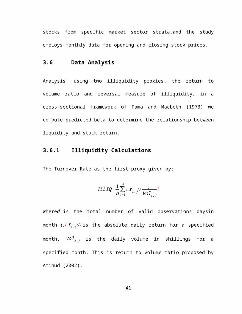
(2014, July 15) https://www.nse.co.ke/regulatory-framework.html
(LVW advisors. Aug 2013) http://www.lvwadvisors.com/wp-content/uploads/2013/09/
(2014, October22) http://data.worldbank.org/indicator/FR.INR.RISK
49

APPENDICES
APPENDIX I: List of Stocks at the NSE as at December 2013
Agricultural Sector
1. Eaagads Limited (EGAD)
2. Kakuzi Limited (KUKZ)
3. Kapchorua Tea Company Limited (KAPC)
4. Limuru Tea Company Limited (LIMT)
5. Rea Vipingo Sisal Estate (REA)
6. Sasini Tea and Coffee (SASN)
7. Williamson Tea Kenya Limited (WTK)
Automobiles and Accessories
8. Car and General Kenya (C&G)
9. CMC Holdings (CMC)
10. Marshalls East Africa (MASH)
11. Sameer Africa Limited (FIRE)
Banking
12. Barclays Bank (Kenya) (BBK)
13. CFC Stanbic Holdings (CFC)
14. Cooperative Bank of Kenya (COOP)
50

15. Diamond Trust Bank Group (DTK)
16. Equity Bank Group (EQTY)
17. Housing Finance Company of Kenya (HFCK)
18. I&M Holdings Limited (I&M)
19. Kenya Commercial Bank Group (KCB)
20. National Bank of Kenya Limited (NBK)
21. National Industrial Credit Bank (NIC)
22. Standard Chartered Kenya(SCBK)
Commercial and Services
23. Express Kenya Limited (XPRS)
24. Kenya Airways Limited (KQ)
25. Longhorn Kenya Limited (LKL)
26. Nation Media Group (NMG)
27. Scangroup (SCAN)
28. Standard Group Limited (SGL)
29. TPS Serena (TPSE)
30. Uchumi Supermarkets (UCHM)
31. Hutchings Biemer Limited (HBL)
Construction and Allied Sector
32. Athi River Mining Limited (ARM)
51

33. Bamburi Cement Limited (BAMB)
34. Crown-Berger(Kenya) (BERG)
35. East African Cables Limited (CABL)
36. East African Portland Cement Company (PORT)
Energy and Petroleum
37. KenolKobil (KENO)
38. Kengen (KEGN)
39. Kenya Power and Lighting Company (KPLC)
40. Total Kenya Limited (TOTL)
41. Umeme (UMME)
Insurance
42. British-America Investment Company (BRIT)
43. CIC Insurance Group (CIC)
44. Jubilee Holdings Limited (JUB)
45. Kenya Reinsurance Corporation (KNRE)
46. Liberty Kenya Holdings (CFCI)
47. Pan Africa Insurance Holdings (PAFR)
Investment
48. Centum Investment Company (ICDC)
52

49. Olympia Capital Holdings (OCH)
50. TransCentury Investments (TCL)
Manufacturing and Allied
51. B.O.C Kenya Limited (BOC)
52. British American Tobacco Limited (BAT)
53. Carbacid Investments Limited (CIL)
54. East African Breweries (EABL)
55. Eveready East Africa (EVRD)
56. Mumias Sugar Company Limited (MSC)
57. Unga Group Limited (UNGA)
58. Kenya Orchards Limited(ORCH)
59. A. Baumann and Company (BAUM)
Telecommunication andTechnology
60. Safaricom (SCOM)
Growth Enterprise Market Segment
61. Home Africa (HAFR)
53

APPENDIX II: Portfolio formation
Table A.1: P1, Portfolio of Largest Size (Deals) at Jan 2009
Month Issuer Deal Volume Turnover Opening Price
Closing Price
Jan SCOM 9,753.00 88,342,944.00 294,244,964.80 3.62 3.20 Jan KCB 3,916.00 22,969,970.00 484,287,059.30 23.77 20.48 Jan COOP 3,430.00 8,743,900.00 81,906,400.00 9.95 8.47 Jan MSC 2,744.00 13,162,978.00 81,494,014.60 6.84 5.02 Jan KEGN 2,067.00 11,636,800.00 183,403,446.60 16.24 14.05 Jan KNRE 1,810.00 4,669,334.00 57,175,006.85 12.80 11.64 Jan EQTY 1,428.00 1,860,004.00 307,303,312.00 188.33 157.32 Jan BBK 1,160.00 1,575,907.00 80,019,789.00 50.83 48.64 Jan KQ 744.00 680,057.00 19,467,209.75 28.78 27.85 Jan HFCK 655.00 905,881.00 15,514,845.15 18.68 16.46
Table A.2: P2, Portfolio of Smallest Size (Deals) at Jan 2009
Month Issuer Deal Volume Turnover Opening Price
Closing Price
Jan KAPC 2.00 300.00 19,800.00 62.00 68.00 Jan C&G 4.00 3,900.00 169,400.00 42.50 40.00 Jan EGAD 10.00 14,200.00 511,850.00 36.44 36.50 Jan PAFR 18.00 11,910.00 671,230.00 62.00 53.25 Jan KUKZ 21.00 19,060.00 439,106.25 23.00 22.00 Jan WTK 30.00 36,150.00 1,881,925.00 52.00 54.00 Jan XPRS 43.00 51,120.00 645,245.00 13.00 11.50 Jan JUB 66.00 32,115.00 3,932,390.00 121.00 130.00 Jan SGL 73.00 85,391.00 4,217,109.00 50.00 45.75 Jan BERG 76.00 41,595.00 1,020,415.00 25.00 22.50
P2 2009 Portfolio of Smallest Size (Deals) at Jan 2009
Table A.3: P3, Portfolio of Largest Volume at Jan 2009
54

Month Issuer Deal Volume Turnover Opening Price
Closing Price
Jan SCOM 9,753.00 88,342,944.00 294,244,964.80 3.62 3.20 Jan KCB 3,916.00 22,969,970.00 484,287,059.30 23.77 20.48 Jan MSC 2,744.00 13,162,978.00 81,494,014.60 6.84 5.02 Jan KEGN 2,067.00 11,636,800.00 183,403,446.60 16.24 14.05 Jan COOP 3,430.00 8,743,900.00 81,906,400.00 9.95 8.47 Jan KNRE 1,810.00 4,669,334.00 57,175,006.85 12.80 11.64 Jan EABL 649.00 2,459,013.00 349,054,354.00 145.33 136.38 Jan EQTY 1,428.00 1,860,004.00 307,303,312.00 188.33 157.32 Jan BBK 1,160.00 1,575,907.00 80,019,789.00 50.83 48.64 Jan HFCK 655.00 905,881.00 15,514,845.15 18.68 16.46
Table A.4: P4, Portfolio of Smallest Volume at Jan 2009
Month Issuer Deal Volume Turnover Opening Price
Closing Price
Jan KAPC 2.00 300.00 19,800.00 62.00 68.00 Jan C&G 4.00 3,900.00 169,400.00 42.50 40.00 Jan PAFR 18.00 11,910.00 671,230.00 62.00 53.25 Jan EGAD 10.00 14,200.00 511,850.00 36.44 36.50 Jan KUKZ 21.00 19,060.00 439,106.25 23.00 22.00 Jan JUB 66.00 32,115.00 3,932,390.00 121.00 130.00 Jan WTK 30.00 36,150.00 1,881,925.00 52.00 54.00 Jan BERG 76.00 41,595.00 1,020,415.00 25.00 22.50 Jan XPRS 43.00 51,120.00 645,245.00 13.00 11.50 Jan SGL 73.00 85,391.00 4,217,109.00 50.00 45.75
P4 2009 Portfolio of Smallest volume at Jan 2009
Table A.5: P5, Portfolio of Largest Turnover at Jan 2009
Month Issuer Deal Volume Turnover Opening Price
Closing Price
Jan KCB 3,916.00 22,969,970.00 484,287,059.30 23.77 20.48 Jan EABL 649.00 2,459,013.00 349,054,354.00 145.33 136.38 Jan EQTY 1,428.00 1,860,004.00 307,303,312.00 188.33 157.32 Jan SCOM 9,753.00 88,342,944.00 294,244,964.80 3.62 3.20 Jan KEGN 2,067.00 11,636,800.00 183,403,446.60 16.24 14.05 Jan COOP 3,430.00 8,743,900.00 81,906,400.00 9.95 8.47 Jan MSC 2,744.00 13,162,978.00 81,494,014.60 6.84 5.02 Jan BAT 114.00 577,326.00 80,189,939.00 131.50 136.25 Jan BBK 1,160.00 1,575,907.00 80,019,789.00 50.83 48.64 Jan KNRE 1,810.00 4,669,334.00 57,175,006.85 12.80 11.64
55

Table A.6: P6, Portfolio of Smallest Turnover at Jan 2009
Month Issuer Deal Volume Turnover Opening Price
Closing Price
Jan KAPC 2.00 300.00 19,800.00 62.00 68.00 Jan C&G 4.00 3,900.00 169,400.00 42.50 40.00 Jan KUKZ 21.00 19,060.00 439,106.25 23.00 22.00 Jan EGAD 10.00 14,200.00 511,850.00 36.44 36.50 Jan XPRS 43.00 51,120.00 645,245.00 13.00 11.50 Jan PAFR 18.00 11,910.00 671,230.00 62.00 53.25 Jan BERG 76.00 41,595.00 1,020,415.00 25.00 22.50 Jan FIRE 185.00 184,375.00 1,093,059.50 5.74 5.91 Jan OCH 86.00 133,300.00 1,296,790.00 9.60 9.03 Jan EVRD 437.00 455,100.00 1,530,315.00 3.53 3.21
P6 2009 Portfolio of Smallest Turnover at Jan 2009
Table A.7:P7, Portfolio of Largest Size (Deals) at Jan 2010
Month Issuer Deal Volume Turnover Opening Price
Closing Price
Jan SCOM 11,496.00 430,267,186.00 2,363,152,327.85 4.57 5.34 Jan MSC 3,268.00 25,967,546.00 224,907,814.85 6.92 8.97 Jan EQTY 3,157.00 66,028,659.00 1,098,417,596.90 14.32 16.02 Jan COOP 3,005.00 16,939,400.00 163,207,030.00 9.03 9.76 Jan KCB 2,277.00 15,559,934.00 345,071,017.75 20.46 22.14 Jan KEGN 1,915.00 4,753,822.00 68,921,977.15 13.01 14.30 Jan KNRE 1,846.00 3,245,032.00 42,636,562.50 11.69 12.52 Jan KQ 1,650.00 9,238,995.00 484,773,925.50 35.93 50.38 Jan BBK 1,055.00 2,560,536.00 128,527,820.25 45.65 49.58 Jan ICDC 593.00 3,345,713.00 43,447,464.65 11.35 13.22
Table A.8:P8, Portfolio of Smallest Size (Deals) at Jan 2010
Month Issuer Deal Volume Turnover Opening Price
Closing Price
Jan EGAD 2.00 200.00 4,200.00 21.00 21.00 Jan KAPC 2.00 460.00 42,960.00 94.50 86.00 Jan C&G 8.00 13,282.00 464,978.50 31.75 34.94 Jan KUKZ 9.00 14,182.00 457,646.00 32.00 34.00 Jan PAFR 21.00 26,192.00 1,202,748.00 45.00 48.00 Jan BERG 43.00 34,800.00 877,125.00 24.00 25.50 Jan XPRS 63.00 72,717.00 633,253.25 7.25 9.00 Jan BAMB 80.00 390,713.00 62,431,349.00 158.00 155.00 Jan SGL 80.00 85,887.00 3,167,058.75 37.00 38.08 Jan OCH 87.00 161,800.00 1,103,980.00 6.20 7.40
Table A.9:P9, Portfolio of Largest Volume at Jan 2010
56

Month Issuer Deal Volume Turnover Opening Price
Closing Price
Jan SCOM 11,496.00 430,267,186.00 2,363,152,327.85 4.57 5.34 Jan EQTY 3,157.00 66,028,659.00 1,098,417,596.90 14.32 16.02 Jan MSC 3,268.00 25,967,546.00 224,907,814.85 6.92 8.97 Jan COOP 3,005.00 16,939,400.00 163,207,030.00 9.03 9.76 Jan KCB 2,277.00 15,559,934.00 345,071,017.75 20.46 22.14 Jan KQ 1,650.00 9,238,995.00 484,773,925.50 35.93 50.38 Jan KEGN 1,915.00 4,753,822.00 68,921,977.15 13.01 14.30 Jan ICDC 593.00 3,345,713.00 43,447,464.65 11.35 13.22 Jan KNRE 1,846.00 3,245,032.00 42,636,562.50 11.69 12.52 Jan BBK 1,055.00 2,560,536.00 128,527,820.25 45.65 49.58
57

Table A.10:P10, Portfolio of Smallest Volume at Jan 2010
Month Issuer Deal Volume Turnover Opening Price
Closing Price
Jan EGAD 2.00 200.00 4,200.00 21.00 21.00 Jan KAPC 2.00 460.00 42,960.00 94.50 86.00 Jan C&G 8.00 13,282.00 464,978.50 31.75 34.94 Jan KUKZ 9.00 14,182.00 457,646.00 32.00 34.00 Jan PAFR 21.00 26,192.00 1,202,748.00 45.00 48.00 Jan BERG 43.00 34,800.00 877,125.00 24.00 25.50 Jan XPRS 63.00 72,717.00 633,253.25 7.25 9.00 Jan SGL 80.00 85,887.00 3,167,058.75 37.00 38.08 Jan DTK 125.00 131,856.00 9,485,769.50 65.00 71.50 Jan UNGA 80.00 141,243.00 1,295,240.50 9.11 9.10
P4 2010 Portfolio of Smallest volume at Jan 2010
Table A.11:P11, Portfolio of Largest Turnover at Jan 2010
Month Issuer Deal Volume Turnover Opening Price
Closing Price
Jan SCOM 11,496.00 430,267,186.00 2,363,152,327.85 4.57 5.34 Jan EQTY 3,157.00 66,028,659.00 1,098,417,596.90 14.32 16.02 Jan KQ 1,650.00 9,238,995.00 484,773,925.50 35.93 50.38 Jan KCB 2,277.00 15,559,934.00 345,071,017.75 20.46 22.14 Jan BAT 207.00 1,877,301.00 328,791,952.00 175.43 175.50 Jan EABL 476.00 1,814,642.00 274,030,403.00 145.60 150.43 Jan MSC 3,268.00 25,967,546.00 224,907,814.85 6.92 8.97 Jan COOP 3,005.00 16,939,400.00 163,207,030.00 9.03 9.76 Jan BBK 1,055.00 2,560,536.00 128,527,820.25 45.65 49.58 Jan KPLC 310.00 602,226.00 88,964,069.00 140.88 149.00
Table A.12:P12, Portfolio of Smallest Turnover at Jan 2010
Month Issuer Deal Volume Turnover Opening Price
Closing Price
Jan EGAD 2.00 200.00 4,200.00 21.00 21.00 Jan KAPC 2.00 460.00 42,960.00 94.50 86.00 Jan KUKZ 9.00 14,182.00 457,646.00 32.00 34.00 Jan C&G 8.00 13,282.00 464,978.50 31.75 34.94 Jan XPRS 63.00 72,717.00 633,253.25 7.25 9.00 Jan BERG 43.00 34,800.00 877,125.00 24.00 25.50 Jan OCH 87.00 161,800.00 1,103,980.00 6.20 7.40 Jan PAFR 21.00 26,192.00 1,202,748.00 45.00 48.00 Jan UNGA 80.00 141,243.00 1,295,240.50 9.11 9.10 Jan EVRD 556.00 825,488.00 3,099,034.80 2.90 3.78
58

Table A.13: P13, Portfolio of Largest Size (Deals) at Jan 2011
Month Issuer Deal Volume Turnover Opening Price
Closing Price
Jan SCOM 6,233.00 470,963,632.00 2,183,587,572.60 4.70 4.48 Jan KPLC 5,276.00 44,570,864.00 1,021,608,775.00 25.73 24.15 Jan COOP 4,948.00 35,034,743.00 706,968,366.30 19.38 20.44 Jan EQTY 3,555.00 40,521,198.00 1,180,470,747.25 27.17 29.07 Jan KCB 3,405.00 39,308,650.00 932,261,778.00 22.05 23.10 Jan MSC 2,560.00 17,681,830.00 175,134,300.70 9.64 8.83 Jan KEGN 2,165.00 9,543,438.00 160,356,806.15 16.87 16.46 Jan KNRE 1,465.00 2,553,672.00 29,014,924.30 10.84 11.06 Jan ICDC 1,338.00 4,156,951.00 99,368,446.50 23.18 23.72 Jan KENO 1,288.00 13,575,950.00 136,563,450.00 10.06 9.99
Table A.14:P14, Portfolio of Smallest Size (Deals) at Jan 2011
Month Issuer Deal Volume Turnover Opening Price
Closing Price
Jan KAPC 14.00 7,000.00 904,800.00 110.00 130.00 Jan PAFR 31.00 26,000.00 1,758,650.00 72.00 63.50 Jan EGAD 41.00 18,800.00 999,800.00 52.33 57.00 Jan C&G 46.00 95,900.00 4,868,700.00 45.50 54.50 Jan WTK 49.00 95,800.00 20,112,200.00 185.00 200.00 Jan KUKZ 66.00 131,266.00 10,808,500.00 81.50 81.00 Jan XPRS 76.00 166,081.00 1,337,787.50 7.75 8.02 Jan BERG 76.00 88,800.00 2,937,800.00 33.00 34.57 Jan BAT 80.00 517,029.00 144,110,564.00 277.00 276.50 Jan JUB 107.00 106,150.00 20,995,236.00 191.33 195.25
Table A.15:P15, Portfolio of Largest Volume at Jan 2011
Month Issuer Deal Volume Turnover Opening Price
Closing Price
Jan SCOM 6,233.00 470,963,632.00 2,183,587,572.60 4.70 4.48 Jan KPLC 5,276.00 44,570,864.00 1,021,608,775.00 25.73 24.15 Jan EQTY 3,555.00 40,521,198.00 1,180,470,747.25 27.17 29.07 Jan KCB 3,405.00 39,308,650.00 932,261,778.00 22.05 23.10 Jan COOP 4,948.00 35,034,743.00 706,968,366.30 19.38 20.44 Jan MSC 2,560.00 17,681,830.00 175,134,300.70 9.64 8.83 Jan KENO 1,288.00 13,575,950.00 136,563,450.00 10.06 9.99 Jan KEGN 2,165.00 9,543,438.00 160,356,806.15 16.87 16.46 Jan KQ 978.00 5,113,439.00 236,127,182.00 46.94 45.76 Jan ICDC 1,338.00 4,156,951.00 99,368,446.50 23.18 23.72
P3 2011 Portfolio of Largest volume at Jan 2011
59

Table A.16:P16, Portfolio of Smallest Volume at Jan 2011
Month Issuer Deal Volume Turnover Opening Price
Closing Price
Jan KAPC 14.00 7,000.00 904,800.00 110.00 130.00 Jan EGAD 41.00 18,800.00 999,800.00 52.33 57.00 Jan PAFR 31.00 26,000.00 1,758,650.00 72.00 63.50 Jan SGL 87.00 56,981.00 2,480,779.75 45.25 42.25 Jan BERG 76.00 88,800.00 2,937,800.00 33.00 34.57 Jan WTK 49.00 95,800.00 20,112,200.00 185.00 200.00 Jan C&G 46.00 95,900.00 4,868,700.00 45.50 54.50 Jan JUB 107.00 106,150.00 20,995,236.00 191.33 195.25 Jan KUKZ 66.00 131,266.00 10,808,500.00 81.50 81.00 Jan XPRS 76.00 166,081.00 1,337,787.50 7.75 8.02
Table A.17:P17, Portfolio of Largest Turnover at Jan 2011
Month Issuer Deal Volume Turnover Opening Price
Closing Price
Jan SCOM 6,233.00 470,963,632.00 2,183,587,572.60 4.70 4.48 Jan EQTY 3,555.00 40,521,198.00 1,180,470,747.25 27.17 29.07 Jan KPLC 5,276.00 44,570,864.00 1,021,608,775.00 25.73 24.15 Jan KCB 3,405.00 39,308,650.00 932,261,778.00 22.05 23.10 Jan COOP 4,948.00 35,034,743.00 706,968,366.30 19.38 20.44 Jan EABL 651.00 2,922,484.00 615,721,377.00 207.11 184.98 Jan NMG 382.00 2,006,078.00 347,644,751.00 161.00 168.42 Jan BBK 1,269.00 4,080,137.00 265,901,786.50 64.02 63.05 Jan KQ 978.00 5,113,439.00 236,127,182.00 46.94 45.76 Jan MSC 2,560.00 17,681,830.00 175,134,300.70 9.64 8.83
Table A.18:P18, Portfolio of Smallest Turnover at Jan 2011
Month Issuer Deal Volume Turnover Opening Price
Closing Price
Jan KAPC 14.00 7,000.00 904,800.00 110.00 130.00 Jan EGAD 41.00 18,800.00 999,800.00 52.33 57.00 Jan XPRS 76.00 166,081.00 1,337,787.50 7.75 8.02 Jan PAFR 31.00 26,000.00 1,758,650.00 72.00 63.50 Jan EVRD 600.00 705,000.00 2,108,230.00 3.17 2.80 Jan SGL 87.00 56,981.00 2,480,779.75 45.25 42.25 Jan OCH 158.00 435,800.00 2,603,460.00 5.97 5.87 Jan BERG 76.00 88,800.00 2,937,800.00 33.00 34.57 Jan UNGA 153.00 406,761.00 4,495,382.75 10.72 11.03 Jan C&G 46.00 95,900.00 4,868,700.00 45.50 54.50
60

Table A.19: P19, Portfolio of Largest Size (Deals) at Jan 2012
Month Issuer Deal Volume Turnover Opening Price
Closing Price
Jan SCOM 2,574.00 201,053,543.00 645,727,030.70 2.97 3.22 Jan EQTY 2,119.00 65,811,930.00 1,075,366,128.45 16.73 17.74 Jan BBK 1,940.00 14,343,283.00 179,004,969.00 13.11 12.37 Jan KCB 1,875.00 10,390,896.00 182,897,214.75 16.74 19.04 Jan MSC 1,376.00 12,598,050.00 63,790,937.15 5.28 5.03 Jan COOP 1,358.00 11,846,629.00 152,546,306.45 12.51 12.98 Jan KPLC 1,027.00 5,022,351.00 80,629,682.05 17.46 15.50 Jan KEGN 899.00 2,882,392.00 23,500,387.00 8.82 7.97 Jan KQ 739.00 997,558.00 20,136,917.60 20.78 19.59 Jan KENO 516.00 3,768,962.00 37,650,521.10 9.84 10.02
Table A.20: P20, Portfolio of Smallest Size (Deals) at Jan 2012
Month Issuer Deal Volume Turnover Opening Price
Closing Price
Jan KAPC 11.00 4,800.00 571,900.00 118.33 114.00 Jan EGAD 15.00 9,700.00 310,400.00 32.00 32.00 Jan C&G 18.00 13,867.00 341,707.25 22.75 25.00 Jan SGL 29.00 28,158.00 756,335.50 24.75 25.88 Jan BERG 35.00 37,620.00 847,265.00 21.33 26.00 Jan KUKZ 37.00 664,350.00 47,280,525.00 68.17 70.00 Jan WTK 39.00 144,830.00 37,193,260.00 273.33 255.00 Jan XPRS 40.00 106,100.00 401,100.00 4.00 4.00 Jan CFC 52.00 92,870.00 3,785,555.00 40.00 40.13 Jan ARM 61.00 197,475.00 30,874,003.00 157.00 151.00
Table A.21:P21, Portfolio of Largest Volume at Jan 2012
Month Issuer Deal Volume Turnover Opening Price
Closing Price
Jan SCOM 2,574.00 201,053,543.00 645,727,030.70 2.97 3.22 Jan EQTY 2,119.00 65,811,930.00 1,075,366,128.45 16.73 17.74 Jan BBK 1,940.00 14,343,283.00 179,004,969.00 13.11 12.37 Jan MSC 1,376.00 12,598,050.00 63,790,937.15 5.28 5.03 Jan COOP 1,358.00 11,846,629.00 152,546,306.45 12.51 12.98 Jan KCB 1,875.00 10,390,896.00 182,897,214.75 16.74 19.04 Jan KPLC 1,027.00 5,022,351.00 80,629,682.05 17.46 15.50 Jan KENO 516.00 3,768,962.00 37,650,521.10 9.84 10.02 Jan KEGN 899.00 2,882,392.00 23,500,387.00 8.82 7.97 Jan EABL 369.00 2,428,039.00 418,971,155.00 174.69 165.73
P3 2012 Portfolio of Largest volume at Jan 2012
61

Table A.22:P22, Portfolio of Smallest Volume at Jan 2012
Month Issuer Deal Volume Turnover Opening Price
Closing Price
Jan KAPC 11.00 4,800.00 571,900.00 118.33 114.00 Jan EGAD 15.00 9,700.00 310,400.00 32.00 32.00 Jan C&G 18.00 13,867.00 341,707.25 22.75 25.00 Jan SGL 29.00 28,158.00 756,335.50 24.75 25.88 Jan BERG 35.00 37,620.00 847,265.00 21.33 26.00 Jan JUB 74.00 49,949.00 7,686,763.00 153.00 149.80 Jan OCH 70.00 72,000.00 245,350.00 3.38 3.35 Jan UNGA 83.00 85,140.00 788,048.00 9.50 9.10 Jan CFC 52.00 92,870.00 3,785,555.00 40.00 40.13 Jan XPRS 40.00 106,100.00 401,100.00 4.00 4.00
P4 2012 Portfolio of Smallest volume at Jan 2012
Table A.23:P23, Portfolio of Largest Turnover at Jan 2012
Month Issuer Deal Volume Turnover Opening Price
Closing Price
Jan EQTY 2,119.00 65,811,930.00 1,075,366,128.45 16.73 17.74 Jan SCOM 2,574.00 201,053,543.00 645,727,030.70 2.97 3.22 Jan EABL 369.00 2,428,039.00 418,971,155.00 174.69 165.73 Jan KCB 1,875.00 10,390,896.00 182,897,214.75 16.74 19.04 Jan BBK 1,940.00 14,343,283.00 179,004,969.00 13.11 12.37 Jan COOP 1,358.00 11,846,629.00 152,546,306.45 12.51 12.98 Jan BAT 65.00 461,513.00 119,123,534.00 247.00 260.00 Jan SCAN 257.00 2,408,499.00 97,283,343.50 41.71 39.50 Jan KPLC 1,027.00 5,022,351.00 80,629,682.05 17.46 15.50 Jan MSC 1,376.00 12,598,050.00 63,790,937.15 5.28 5.03
P5 2012 Portfolio of Largest Turnover at Jan 2012
Table A.24:P24, Portfolio of Smallest Turnover at Jan 2012
Month Issuer Deal Volume Turnover Opening Price
Closing Price
Jan OCH 70.00 72,000.00 245,350.00 3.38 3.35 Jan EGAD 15.00 9,700.00 310,400.00 32.00 32.00 Jan C&G 18.00 13,867.00 341,707.25 22.75 25.00 Jan XPRS 40.00 106,100.00 401,100.00 4.00 4.00 Jan KAPC 11.00 4,800.00 571,900.00 118.33 114.00 Jan SGL 29.00 28,158.00 756,335.50 24.75 25.88 Jan UNGA 83.00 85,140.00 788,048.00 9.50 9.10 Jan BERG 35.00 37,620.00 847,265.00 21.33 26.00 Jan EVRD 263.00 595,200.00 1,014,915.00 1.79 1.66 Jan TOTL 115.00 130,680.00 2,021,030.00 14.63 16.20
62

Table A.25:P25, Portfolio of Largest Size (Deals) at Jan 2013
Month Issuer Deal Volume Turnover Opening Price
Closing Price
Jan SCOM 5,255.00 264,272,995.00 1,479,296,290.90 5.08 5.45 Jan KCB 2,882.00 34,100,049.00 1,115,507,090.00 30.04 33.42 Jan KEGN 2,284.00 21,491,381.00 253,656,293.05 8.76 11.75 Jan BBK 1,956.00 17,230,731.00 275,153,028.15 15.68 16.13 Jan MSC 1,949.00 33,309,463.00 167,803,126.70 4.91 5.04 Jan COOP 1,842.00 15,942,891.00 206,956,039.35 12.74 12.84 Jan EQTY 1,418.00 15,216,305.00 396,700,013.75 23.88 26.33 Jan KPLC 947.00 12,387,233.00 215,920,869.50 17.03 17.44 Jan KNRE 911.00 3,157,677.00 37,215,248.00 10.54 11.73 Jan NIC 792.00 3,183,834.00 138,216,026.00 38.54 41.94
P1 2013 Portfolio of Largest Size (Deals) at Jan 2013
Table A.26:P26, Portfolio of Smallest Size (Deals) at Jan 2013
Month Issuer Deal Volume Turnover Opening Price
Closing Price
Jan KUKZ 18.00 109,358.00 7,683,687.00 67.50 71.00 Jan KAPC 19.00 6,200.00 724,900.00 118.00 112.50 Jan C&G 26.00 26,581.00 649,007.00 24.25 24.00 Jan XPRS 35.00 40,210.00 135,694.50 3.47 3.50 Jan OCH 40.00 90,800.00 328,965.00 3.70 3.60 Jan WTK 43.00 32,662.00 6,527,260.00 200.00 200.00 Jan BERG 46.00 128,900.00 5,461,175.00 41.91 42.50 Jan SGL 67.00 102,560.00 2,382,450.75 22.50 21.85 Jan EGAD 72.00 84,600.00 1,990,625.00 23.75 24.00 Jan JUB 103.00 161,644.00 30,609,442.00 174.75 187.00
Table A.27:P27, Portfolio of Largest Volume at Jan 2013
Month Issuer Deal Volume Turnover Opening Price
Closing Price
Jan SCOM 5,255.00 264,272,995.00 1,479,296,290.90 5.08 5.45 Jan KCB 2,882.00 34,100,049.00 1,115,507,090.00 30.04 33.42 Jan MSC 1,949.00 33,309,463.00 167,803,126.70 4.91 5.04 Jan KEGN 2,284.00 21,491,381.00 253,656,293.05 8.76 11.75 Jan BBK 1,956.00 17,230,731.00 275,153,028.15 15.68 16.13 Jan COOP 1,842.00 15,942,891.00 206,956,039.35 12.74 12.84 Jan EQTY 1,418.00 15,216,305.00 396,700,013.75 23.88 26.33 Jan KPLC 947.00 12,387,233.00 215,920,869.50 17.03 17.44 Jan KENO 381.00 12,113,131.00 165,994,496.20 13.57 13.63 Jan EABL 678.00 5,029,203.00 1,493,760,265.00 267.00 301.20
63

Table A.28:P28, Portfolio of Smallest Volume at Jan 2013
Month Issuer Deal Volume Turnover Opening Price
Closing Price
Jan KAPC 19.00 6,200.00 724,900.00 118.00 112.50 Jan C&G 26.00 26,581.00 649,007.00 24.25 24.00 Jan WTK 43.00 32,662.00 6,527,260.00 200.00 200.00 Jan XPRS 35.00 40,210.00 135,694.50 3.47 3.50 Jan EGAD 72.00 84,600.00 1,990,625.00 23.75 24.00 Jan OCH 40.00 90,800.00 328,965.00 3.70 3.60 Jan SGL 67.00 102,560.00 2,382,450.75 22.50 21.85 Jan KUKZ 18.00 109,358.00 7,683,687.00 67.50 71.00 Jan BERG 46.00 128,900.00 5,461,175.00 41.91 42.50 Jan JUB 103.00 161,644.00 30,609,442.00 174.75 187.00
Table A.29:P29, Portfolio of Largest Turnover at Jan 2013
Month Issuer Deal Volume Turnover Opening Price
Closing Price
Jan EABL 678.00 5,029,203.00 1,493,760,265.00 267.00 301.20 Jan SCOM 5,255.00 264,272,995.00 1,479,296,290.90 5.08 5.45 Jan KCB 2,882.00 34,100,049.00 1,115,507,090.00 30.04 33.42 Jan EQTY 1,418.00 15,216,305.00 396,700,013.75 23.88 26.33 Jan BAT 182.00 732,385.00 386,419,443.00 500.00 515.86 Jan BBK 1,956.00 17,230,731.00 275,153,028.15 15.68 16.13 Jan KEGN 2,284.00 21,491,381.00 253,656,293.05 8.76 11.75 Jan ARM 551.00 4,287,831.00 231,284,806.00 49.93 52.15 Jan NMG 317.00 888,689.00 221,656,392.00 220.75 259.30 Jan KPLC 947.00 12,387,233.00 215,920,869.50 17.03 17.44
P5 2013 Portfolio of Largest Turnover at Jan 2013
Table A.30: P30, Portfolio of Smallest Turnover at Jan 2013
64

Month Issuer Deal Volume Turnover Opening Price
Closing Price
Jan XPRS 35.00 40,210.00 135,694.50 3.47 3.50 Jan OCH 40.00 90,800.00 328,965.00 3.70 3.60 Jan C&G 26.00 26,581.00 649,007.00 24.25 24.00 Jan KAPC 19.00 6,200.00 724,900.00 118.00 112.50 Jan EVRD 368.00 565,511.00 1,107,185.40 2.04 1.96 Jan EGAD 72.00 84,600.00 1,990,625.00 23.75 24.00 Jan SGL 67.00 102,560.00 2,382,450.75 22.50 21.85 Jan UNGA 118.00 346,413.00 4,753,317.30 13.05 13.67 Jan BERG 46.00 128,900.00 5,461,175.00 41.91 42.50 Jan TOTL 155.00 423,551.00 5,880,333.00 13.86 13.82
P6 2013 Portfolio of Smallest Turnover at Jan 2013
APPENDIX III: Cross-sectional testing results under 2ndILLQ measure
65

Table A 31: Summary output of Cross-sectional testing under 2nd ILLQ measure
Regression Statistics Multiple R R Square Adjusted R
SquareStandard
Error Observations
P1 0.78 0.62 0.59 0.08 60.00 P2 0.81 0.65 0.62 0.06 60.00 P3 0.79 0.63 0.60 0.07 60.00 P4 0.81 0.65 0.62 0.06 60.00 P5 0.80 0.63 0.60 0.06 60.00 P6 0.81 0.65 0.62 0.06 60.00 P7 0.79 0.62 0.59 0.08 60.00 P8 0.87 0.75 0.72 0.05 60.00 P9 0.78 0.61 0.58 0.08 60.00 P10 0.78 0.61 0.58 0.06 60.00 P11 0.79 0.62 0.59 0.06 60.00 P12 0.81 0.65 0.62 0.06 60.00 P13 0.73 0.53 0.50 0.10 60.00 P14 0.83 0.70 0.67 0.05 60.00 P15 0.74 0.55 0.52 0.10 60.00 P16 0.82 0.68 0.65 0.06 60.00 P17 0.81 0.65 0.62 0.07 60.00 P18 0.83 0.69 0.66 0.05 60.00 P19 0.76 0.58 0.55 0.09 60.00 P20 0.74 0.54 0.51 0.07 60.00 P21 0.78 0.61 0.58 0.08 60.00 P22 0.83 0.69 0.67 0.05 60.00 P23 0.79 0.62 0.59 0.06 60.00 P24 0.85 0.73 0.70 0.05 60.00 P25 0.75 0.57 0.53 0.09 60.00 P26 0.82 0.66 0.64 0.06 60.00 P27 0.78 0.61 0.58 0.08 60.00 P28 0.82 0.66 0.64 0.06 60.00 P29 0.82 0.67 0.65 0.06 60.00 P30 0.85 0.73 0.70 0.05 60.00
Number of data points per portfolio is 60; Standard Error is less or equal to 0.1 for
majority of the portfolios; R-squared for the 30 portfolios are greater than 50% under the
2nd Illiquidity measure; Adjusted R-squared are also greater than 50%.
66

Table A32 a:ANOVA of Cross-sectional testing under 2nd ILLQ measure, P1 to P15
df SS MS F Significance FRegression 3.00 0.56 0.19 30.49 0.00 Residual 57.00 0.35 0.01 Total 60.00 0.92 Regression 3.00 0.40 0.13 35.76 0.00 Residual 57.00 0.21 0.00 Total 60.00 0.61 Regression 3.00 0.45 0.15 32.52 0.00 Residual 57.00 0.27 0.00 Total 60.00 0.72 Regression 3.00 0.40 0.13 35.76 0.00 Residual 57.00 0.21 0.00 Total 60.00 0.61 Regression 3.00 0.33 0.11 32.76 0.00 Residual 57.00 0.19 0.00 Total 60.00 0.52 Regression 3.00 0.36 0.12 37.03 0.00 Residual 57.00 0.18 0.00 Total 60.00 0.54 Regression 3.00 0.58 0.19 30.56 0.00 Residual 57.00 0.36 0.01 Total 60.00 0.94 Regression 3.00 0.37 0.12 56.87 0.00 Residual 57.00 0.12 0.00 Total 60.00 0.49 Regression 3.00 0.57 0.19 29.58 0.00 Residual 57.00 0.37 0.01 Total 60.00 0.94 Regression 3.00 0.32 0.11 30.16 0.00 Residual 57.00 0.20 0.00 Total 60.00 0.52 Regression 3.00 0.38 0.13 31.57 0.00 Residual 57.00 0.23 0.00 Total 60.00 0.61 Regression 3.00 0.35 0.12 35.03 0.00 Residual 57.00 0.19 0.00 Total 60.00 0.54 Regression 3.00 0.64 0.21 21.49 0.00 Residual 57.00 0.56 0.01 Total 60.00 1.20 Regression 3.00 0.33 0.11 43.72 0.00 Residual 57.00 0.14 0.00 Total 60.00 0.47 Regression 3.00 0.64 0.21 23.26 0.00 Residual 57.00 0.52 0.01 Total 60.00 1.16
P13
P14
P15
P7
P8
P9
P10
P11
P12
P1
P2
P3
P4
P5
P6
These portfolios have 3 degrees of freedom; regression sum squared and residual sum squared are for the majority of the cases less than 0.5; the F-test reveals p-values well below 0.5%.
67

Table A32 b:ANOVA of Cross-sectional testing under 2nd ILLQ measure, P16 to
P30
df SS MS F Significance FRegression 3.00 0.42 0.14 40.09 0.00 Residual 57.00 0.20 0.00 Total 60.00 0.61 Regression 3.00 0.49 0.16 35.39 0.00 Residual 57.00 0.26 0.00 Total 60.00 0.75 Regression 3.00 0.38 0.13 41.63 0.00 Residual 57.00 0.17 0.00 Total 60.00 0.55 Regression 3.00 0.67 0.22 26.30 0.00 Residual 57.00 0.49 0.01 Total 60.00 1.16 Regression 3.00 0.35 0.12 22.64 0.00 Residual 57.00 0.30 0.01 Total 60.00 0.65 Regression 3.00 0.54 0.18 29.94 0.00 Residual 57.00 0.35 0.01 Total 60.00 0.89 Regression 3.00 0.35 0.12 43.14 0.00 Residual 57.00 0.16 0.00 Total 60.00 0.51 Regression 3.00 0.37 0.12 30.84 0.00 Residual 57.00 0.23 0.00 Total 60.00 0.60 Regression 3.00 0.39 0.13 50.52 0.00 Residual 57.00 0.15 0.00 Total 60.00 0.54 Regression 3.00 0.63 0.21 24.82 0.00 Residual 57.00 0.48 0.01 Total 60.00 1.12 Regression 3.00 0.41 0.14 37.70 0.00 Residual 57.00 0.21 0.00 Total 60.00 0.62 Regression 3.00 0.54 0.18 29.94 0.00 Residual 57.00 0.35 0.01 Total 60.00 0.89 Regression 3.00 0.41 0.14 37.70 0.00 Residual 57.00 0.21 0.00 Total 60.00 0.62 Regression 3.00 0.37 0.12 39.35 0.00 Residual 57.00 0.18 0.00 Total 60.00 0.55 Regression 3.00 0.39 0.13 50.52 0.00 Residual 57.00 0.15 0.00 Total 60.00 0.54
P25
P26
P27
P28
P29
P30
P19
P20
P21
P22
P23
P24
P16
P17
P18
These portfolios have 3 degrees of freedom; regression sum squared and residual sum squared are for the majority of the cases less than 0.5; the F-test reveals p-values well below 0.5%.
68

Table A33 a:Result of Coefficients, for Cross-sectional testing under 2nd ILLQ
measure, P1 to P10
Coefficients Standard Error t Stat P-value Lower
95%Upper 95%
Intercept - RM-RFR 0.47 0.12 3.75 0.00 0.22 0.72 Volume 0.00 0.00 1.88 0.07 (0.00) 0.00 2ndIlliquidity measure x10^-9 (0.05) 0.01 (3.29) 0.00 (0.07) (0.02) Intercept - RM-RFR 0.59 0.10 5.84 0.00 0.39 0.79 Volume (0.00) 0.00 (0.12) 0.90 (0.00) 0.00 2ndIlliquidity measure x10^-9 (0.00) 0.00 (1.41) 0.16 (0.00) 0.00 Intercept - RM-RFR 0.48 0.11 4.40 0.00 0.26 0.69 Volume 0.00 0.00 0.53 0.60 (0.00) 0.00 2ndIlliquidity measure x10^-9 (0.02) 0.01 (2.13) 0.04 (0.03) (0.00) Intercept - RM-RFR 0.59 0.10 5.84 0.00 0.39 0.79 Volume (0.00) 0.00 (0.12) 0.90 (0.00) 0.00 2ndIlliquidity measure x10^-9 (0.00) 0.00 (1.41) 0.16 (0.00) 0.00 Intercept - RM-RFR 0.37 0.09 4.06 0.00 0.19 0.56 Volume 0.00 0.00 0.25 0.80 (0.00) 0.00 2ndIlliquidity measure x10^-9 (0.01) 0.01 (1.96) 0.05 (0.02) 0.00 Intercept - RM-RFR 0.26 0.09 2.80 0.01 0.07 0.45 Volume 0.00 0.00 1.99 0.05 (0.00) 0.00 2ndIlliquidity measure x10^-9 (0.00) 0.00 (4.39) 0.00 (0.00) (0.00) Intercept - RM-RFR 0.49 0.13 3.89 0.00 0.24 0.74 Volume 0.00 0.00 2.15 0.04 0.00 0.00 2ndIlliquidity measure x10^-9 (0.05) 0.01 (3.45) 0.00 (0.08) (0.02) Intercept - RM-RFR 0.32 0.08 4.28 0.00 0.17 0.47 Volume (0.00) 0.00 (0.19) 0.85 (0.00) 0.00 2nd Illiquidity measure (0.00) 0.00 (3.44) 0.00 (0.00) (0.00) Intercept - RM-RFR 0.50 0.13 3.94 0.00 0.25 0.76 Volume 0.00 0.00 1.85 0.07 (0.00) 0.00 2ndIlliquidity measure x10^-9 (0.04) 0.01 (3.23) 0.00 (0.07) (0.02) Intercept - RM-RFR 0.26 0.09 2.73 0.01 0.07 0.45 Volume (0.00) 0.00 (0.41) 0.69 (0.00) 0.00 2ndIlliquidity measure x10^-9 (0.00) 0.00 (3.01) 0.00 (0.00) (0.00)
P7
P8
P9
P10
P1
P2
P3
P4
P5
P6
For the tested portfolios, the intercept for the regression run is taken to be zero, variables under observations are 2ndilliquidity measure, volume traded and market returns.
69

Table A33 b:Result of Coefficients, for Cross-sectional testing under 2nd ILLQ measure, P11 to P20
Coefficients Standard Error t Stat P-value Lower
95%Upper 95%
Intercept - RM-RFR 0.44 0.10 4.40 0.00 0.24 0.64 Volume 0.00 0.00 0.02 0.98 (0.00) 0.00 2ndIlliquidity measure x10^-9 (0.01) 0.00 (1.58) 0.12 (0.02) 0.00 Intercept - RM-RFR 0.29 0.09 3.12 0.00 0.10 0.47 Volume 0.00 0.00 1.30 0.20 (0.00) 0.00 2ndIlliquidity measure x10^-9 (0.00) 0.00 (3.85) 0.00 (0.00) (0.00) Intercept - RM-RFR 0.60 0.16 3.83 0.00 0.29 0.92 Volume 0.00 0.00 1.22 0.23 (0.00) 0.00 2ndIlliquidity measure x10^-9 (0.03) 0.01 (2.22) 0.03 (0.05) (0.00) Intercept - RM-RFR 0.47 0.08 5.75 0.00 0.31 0.64 Volume 0.00 0.00 0.87 0.39 (0.00) 0.00 2nd Illiquidity measure x10^-9 (0.00) 0.00 (2.66) 0.01 (0.00) (0.00) Intercept - RM-RFR 0.59 0.15 3.88 0.00 0.28 0.89 Volume 0.00 0.00 1.09 0.28 (0.00) 0.00 2ndIlliquidity measure x10^-9 (0.02) 0.01 (2.28) 0.03 (0.04) (0.00) Intercept - RM-RFR 0.56 0.09 5.99 0.00 0.37 0.75 Volume 0.00 0.00 2.13 0.04 0.00 0.00 2ndIlliquidity measure x10^-9 (0.00) 0.00 (3.26) 0.00 (0.00) (0.00) Intercept - RM-RFR 0.56 0.11 5.19 0.00 0.34 0.77 Volume 0.00 0.00 0.41 0.69 (0.00) 0.00 2ndIlliquidity measure x10^-9 (0.01) 0.01 (1.76) 0.08 (0.02) 0.00 Intercept - RM-RFR 0.24 0.09 2.72 0.01 0.06 0.42 Volume 0.00 0.00 1.35 0.18 (0.00) 0.00 2ndIlliquidity measure x10^-9 (0.00) 0.00 (4.46) 0.00 (0.00) (0.00) Intercept - RM-RFR 0.58 0.15 4.00 0.00 0.29 0.88 Volume 0.00 0.00 1.21 0.23 (0.00) 0.00 2ndIlliquidity measure x10^-9 (0.03) 0.01 (2.44) 0.02 (0.05) (0.00) Intercept - RM-RFR 0.42 0.11 3.73 0.00 0.20 0.65 Volume 0.00 0.00 0.50 0.62 (0.00) 0.00 2nd Illiquidity measure x10^-9 (0.00) 0.00 (3.05) 0.00 (0.00) (0.00)
P19
P20
P13
P14
P15
P16
P17
P18
P11
P12
For the tested portfolios, the intercept for the regression run is taken to be zero, variables under observations are 2nd illiquidity measure, volume traded and market returns.
70

Table A33 c:Result of Coefficients, for Cross-sectional testing under 2nd ILLQ
measure, P21 to P30
Coefficients Standard Error t Stat P-value Lower
95%Upper 95%
Intercept - RM-RFR 0.58 0.12 4.69 0.00 0.33 0.82 Volume 0.00 0.00 0.49 0.62 (0.00) 0.00 2ndIlliquidity measure x10^-9 (0.01) 0.01 (1.84) 0.07 (0.02) 0.00 Intercept - RM-RFR 0.33 0.08 4.00 0.00 0.17 0.50 Volume (0.00) 0.00 (0.99) 0.33 (0.00) 0.00 2ndIlliquidity measure x10^-9 (0.00) 0.00 (4.32) 0.00 (0.00) (0.00) Intercept - RM-RFR 0.43 0.10 4.33 0.00 0.23 0.63 Volume 0.00 0.00 0.03 0.98 (0.00) 0.00 2ndIlliquidity measure x10^-9 (0.01) 0.00 (1.57) 0.12 (0.02) 0.00 Intercept - RM-RFR 0.20 0.08 2.46 0.02 0.04 0.36 Volume 0.00 0.00 2.40 0.02 0.00 0.00 2ndIlliquidity measure x10^-9 (0.00) 0.00 (5.76) 0.00 (0.00) (0.00) Intercept - RM-RFR 0.62 0.15 4.28 0.00 0.33 0.92 Volume 0.00 0.00 1.14 0.26 (0.00) 0.00 2ndIlliquidity measure x10^-9 (0.03) 0.01 (2.15) 0.04 (0.05) (0.00) Intercept - RM-RFR 0.57 0.10 5.96 0.00 0.38 0.76 Volume 0.00 0.00 1.97 0.05 (0.00) 0.00 2nd Illiquidity measure x10^-9 (0.00) 0.00 (3.01) 0.00 (0.00) (0.00) Intercept - RM-RFR 0.58 0.12 4.69 0.00 0.33 0.82 Volume 0.00 0.00 0.49 0.62 (0.00) 0.00 2ndIlliquidity measure x10^-9 (0.01) 0.01 (1.84) 0.07 (0.02) 0.00 Intercept - RM-RFR 0.57 0.10 5.96 0.00 0.38 0.76 Volume 0.00 0.00 1.97 0.05 (0.00) 0.00 2ndIlliquidity measure x10^-9 (0.00) 0.00 (3.01) 0.00 (0.00) (0.00) Intercept - RM-RFR 0.41 0.09 4.63 0.00 0.23 0.59 Volume 0.00 0.00 0.15 0.88 (0.00) 0.00 2ndIlliquidity measure x10^-9 (0.01) 0.00 (2.10) 0.04 (0.01) (0.00) Intercept - RM-RFR 0.20 0.08 2.46 0.02 0.04 0.36 Volume 0.00 0.00 2.40 0.02 0.00 0.00 2ndIlliquidity measure x10^-9 (0.00) 0.00 (5.76) 0.00 (0.00) (0.00)
P25
P26
P27
P28
P29
P30
P21
P22
P23
P24
For the tested portfolios, the intercept for the regression run is taken to be zero, variables
under observations are 2nd illiquidity measure, volume traded and market returns.
71