DecisionTreeClassificationand ...746332/FULLTEXT01.pdf · DecisionTreeClassificationand...
79
Decision Tree Classification and Forecasting of Pricing Time Series Data EMIL LUNDKVIST Master’s Degree Project Stockholm, Sweden July 2014 TRITA-XR-EE-RT 2014:017
-
Upload
trinhthuan -
Category
Documents
-
view
220 -
download
0
Transcript of DecisionTreeClassificationand ...746332/FULLTEXT01.pdf · DecisionTreeClassificationand...

Decision Tree Classification andForecasting of Pricing Time Series Data
EMIL LUNDKVIST
Master’s Degree ProjectStockholm, Sweden July 2014
TRITA-XR-EE-RT 2014:017


AbstractMany companies today, in different fields of operations and sizes, have accessto a vast amount of data which was not available only a couple of years ago.This situation gives rise to questions regarding how to organize and use thedata in the best way possible.
In this thesis a large database of pricing data for products within various marketsegments is analysed. The pricing data is from both external and internalsources and is therefore confidential. Because of the confidentiality, the labelsfrom the database are in this thesis substituted with generic ones and thecompany is not referred to by name, but the analysis is carried out on thereal data set. The data is from the beginning unstructured and difficult tooverlook. Therefore, it is first classified. This is performed by feeding somemanual training data into an algorithm which builds a decision tree. Thedecision tree is used to divide the rest of the products in the database intoclasses. Then, for each class, a multivariate time series model is built and eachproduct’s future price within the class can be predicted. In order to interactwith the classification and price prediction, a front end is also developed.
The results show that the classification algorithm both is fast enough to operatein real time and performs well. The time series analysis shows that it is possibleto use the information within each class to do predictions, and a simple vectorautoregressive model used to perform it shows good predictive results.


Acknowledgements
I would like to express my very great appreciation to Daniel Antonsson for giv-ing the opportunity to work with his group and the valuable information he hasshared.
I would also like to extend my thanks to Patricio Valenzuela who has acted as mysupervisor at KTH and provided important knowledge and advice. My gratefulthanks are also extended to Professor Cristian Rojas who is my examiner at KTHand has given his time to help me.
Finally I would like to thank my family for their support during the thesis.

Contents
Glossary
1 Introduction 11.1 Background . . . . . . . . . . . . . . . . . . . . . . . . . . . . . . . . 11.2 Problem Definition and Requirements . . . . . . . . . . . . . . . . . 2
1.2.1 Requirements on the Classification Algorithm . . . . . . . . . 41.2.2 Requirements on the Time Series Analysis . . . . . . . . . . . 41.2.3 Requirements on the Front End Application . . . . . . . . . . 5
1.3 Previous Work . . . . . . . . . . . . . . . . . . . . . . . . . . . . . . 51.4 Outline of the Report . . . . . . . . . . . . . . . . . . . . . . . . . . 6
2 Theory 72.1 Data Structure . . . . . . . . . . . . . . . . . . . . . . . . . . . . . . 72.2 Classification . . . . . . . . . . . . . . . . . . . . . . . . . . . . . . . 9
2.2.1 Choice of Method . . . . . . . . . . . . . . . . . . . . . . . . 102.2.2 Classifying With an Existing Decision Tree . . . . . . . . . . 122.2.3 Building a Decision Tree . . . . . . . . . . . . . . . . . . . . . 13
2.3 Time Series Analysis . . . . . . . . . . . . . . . . . . . . . . . . . . . 182.3.1 Introduction . . . . . . . . . . . . . . . . . . . . . . . . . . . 192.3.2 A Classic Approach . . . . . . . . . . . . . . . . . . . . . . . 25
3 Analysis and Implementation 273.1 Implementation Tools . . . . . . . . . . . . . . . . . . . . . . . . . . 273.2 Classification . . . . . . . . . . . . . . . . . . . . . . . . . . . . . . . 28
3.2.1 Creating a Decision Tree . . . . . . . . . . . . . . . . . . . . . 283.2.2 Storing a Decision Tree . . . . . . . . . . . . . . . . . . . . . 303.2.3 Classifying With a Decision Tree . . . . . . . . . . . . . . . . 30
3.3 Time Series Analysis . . . . . . . . . . . . . . . . . . . . . . . . . . . 313.3.1 Analysis . . . . . . . . . . . . . . . . . . . . . . . . . . . . . . 313.3.2 Implementation . . . . . . . . . . . . . . . . . . . . . . . . . . 36
3.4 Front End . . . . . . . . . . . . . . . . . . . . . . . . . . . . . . . . . 38
4 Results 394.1 Classification . . . . . . . . . . . . . . . . . . . . . . . . . . . . . . . 39

4.1.1 Creating a Decision Tree . . . . . . . . . . . . . . . . . . . . . 394.1.2 Storing a Decision Tree . . . . . . . . . . . . . . . . . . . . . 404.1.3 Classifying With a Decision Tree . . . . . . . . . . . . . . . . 414.1.4 Quality of the Classification . . . . . . . . . . . . . . . . . . . 42
4.2 Time Series Analysis . . . . . . . . . . . . . . . . . . . . . . . . . . . 434.3 Front End . . . . . . . . . . . . . . . . . . . . . . . . . . . . . . . . . 49
4.3.1 Pricing Data . . . . . . . . . . . . . . . . . . . . . . . . . . . 494.3.2 Plot Data . . . . . . . . . . . . . . . . . . . . . . . . . . . . . 49
5 Conclusions 515.1 Future Work . . . . . . . . . . . . . . . . . . . . . . . . . . . . . . . 51
5.1.1 Classification . . . . . . . . . . . . . . . . . . . . . . . . . . . 525.1.2 Time Series Analysis . . . . . . . . . . . . . . . . . . . . . . . 52
Appendices 53
A Front End Manual 55A.1 Introduction . . . . . . . . . . . . . . . . . . . . . . . . . . . . . . . . 55A.2 Interface . . . . . . . . . . . . . . . . . . . . . . . . . . . . . . . . . . 55
A.2.1 Pricing Data . . . . . . . . . . . . . . . . . . . . . . . . . . . 55A.2.2 Plot Data . . . . . . . . . . . . . . . . . . . . . . . . . . . . . 59
A.3 Functions . . . . . . . . . . . . . . . . . . . . . . . . . . . . . . . . . 61A.3.1 Pricing Data . . . . . . . . . . . . . . . . . . . . . . . . . . . 61A.3.2 Plot Data . . . . . . . . . . . . . . . . . . . . . . . . . . . . . 62
Bibliography 65

List of Figures
1.1 Johann Gottfried Galle - A great predictor. . . . . . . . . . . . . . . . . 21.2 Decca Records - A not so great predictor. . . . . . . . . . . . . . . . . . 21.3 Overview of the process. . . . . . . . . . . . . . . . . . . . . . . . . . . . 4
2.1 The structure of the data in the database. . . . . . . . . . . . . . . . . . 72.2 Unsupervised learning. . . . . . . . . . . . . . . . . . . . . . . . . . . . . 92.3 Supervised learning. . . . . . . . . . . . . . . . . . . . . . . . . . . . . . 102.4 Decision tree example. . . . . . . . . . . . . . . . . . . . . . . . . . . . . 132.5 Entropy as a function of the probability of heads for a coin toss. . . . . 162.6 C4.5 example decision tree. . . . . . . . . . . . . . . . . . . . . . . . . . 182.7 Original data and trend. . . . . . . . . . . . . . . . . . . . . . . . . . . . 262.8 Data without trend and seasonal components. . . . . . . . . . . . . . . . 262.9 Autocorrelation of residuals for an AR(9) model. . . . . . . . . . . . . . 262.10 Forecast. . . . . . . . . . . . . . . . . . . . . . . . . . . . . . . . . . . . . 26
3.1 Implementation overview. . . . . . . . . . . . . . . . . . . . . . . . . . . 273.2 Codebook example. . . . . . . . . . . . . . . . . . . . . . . . . . . . . . . 303.3 Table to store decision trees in the database. . . . . . . . . . . . . . . . 303.4 Example price evolution for three products. . . . . . . . . . . . . . . . . 323.5 The ACF of the differentiated example products. . . . . . . . . . . . . . 333.6 Prediction of the example products. . . . . . . . . . . . . . . . . . . . . 343.7 Price evolution for product and mean. . . . . . . . . . . . . . . . . . . . 353.8 The ACF of the differentiated products and mean. . . . . . . . . . . . . 353.9 Prediction of the product and mean. . . . . . . . . . . . . . . . . . . . . 363.10 Time window selection. . . . . . . . . . . . . . . . . . . . . . . . . . . . 38
4.1 Tree build time for different number of products. . . . . . . . . . . . . . 404.2 Tree build time for different number of decision variables. . . . . . . . . 414.3 Classification time for different number of classification products. . . . . 424.4 Classification time for different number of decision variables. . . . . . . 424.5 Model and validation part for product and mean price evolution. . . . . 444.6 Residuals for the mean price with the VAR and simple model. . . . . . 454.7 Residuals for the mean price with the VAR and simple model using a
moving model part. . . . . . . . . . . . . . . . . . . . . . . . . . . . . . . 464.8 Histogram of the absolute residuals for the VAR and simple model. . . . 47

4.9 Resulting p-values for the Granger causality test for 12 test classes with5 products in each class. . . . . . . . . . . . . . . . . . . . . . . . . . . . 47
4.10 Resulting p-value histogram for the Granger causality test for 12 testclasses with 5 products in each class. . . . . . . . . . . . . . . . . . . . . 48
4.11 Front end pricing data. . . . . . . . . . . . . . . . . . . . . . . . . . . . 504.12 Front end plot data. . . . . . . . . . . . . . . . . . . . . . . . . . . . . . 50
A.1 Pricing Data tab. . . . . . . . . . . . . . . . . . . . . . . . . . . . . . . . 56A.2 Plot Data tab. . . . . . . . . . . . . . . . . . . . . . . . . . . . . . . . . 59

List of Tables
2.1 Example of a couple of entries in the database. . . . . . . . . . . . . . . 82.2 Data types in the database. . . . . . . . . . . . . . . . . . . . . . . . . . 92.3 Overview of classification algorithms [14, 20]. . . . . . . . . . . . . . . . 112.4 Description of data type properties. . . . . . . . . . . . . . . . . . . . . 112.5 Decision tree algorithms. . . . . . . . . . . . . . . . . . . . . . . . . . . . 122.6 C4.5 example training data. . . . . . . . . . . . . . . . . . . . . . . . . . 172.7 C4.5 example measures. . . . . . . . . . . . . . . . . . . . . . . . . . . . 18
4.1 Test computer specifications. . . . . . . . . . . . . . . . . . . . . . . . . 404.2 Result of the classification quality test. . . . . . . . . . . . . . . . . . . . 43
A.1 Description of control elements in the Pricing Data tab. . . . . . . . . . 57A.2 Column information in the results view. . . . . . . . . . . . . . . . . . . 58A.3 Description of control elements in the Plot Data tab. . . . . . . . . . . . 60A.4 Navigation in the graph view. . . . . . . . . . . . . . . . . . . . . . . . . 61

Glossary
G(X) The gain criterion of a test X. 14
I(D) The entropy of the training data D. 15
γX(r, s) The covariance function. 19
µX(t) The mean function. 19
θ The number of model parameters. 23
{Xt} A time series. t = 0, . . . , n. 19
{Zt} A time series, usually representing white noise. t = 0, . . . , n. 20
pv The p-value. 44
ACF, ρX(h) The autocorrelation function. 21
ACVF, γX(h) The autocovariance function. 20
AR(p) Autoregressive model of order p. 22
ARMA(p,q) Autoregressive moving average model of order p+ q. 22
MA(q) Moving average model of order q. 22
PACF, αX(h) The partial autocorrelation function. 21
VAR(p) Vector autoregressive model of order p. 22
WN(0, σ2) White noise with mean 0 and variance σ2. 20


Chapter 1
Introduction
1.1 Background
Humans have always been and always will be curious about the future. We have forinstance tried to predict small things such as the outcome of tomorrow’s big soccergame or the upcoming election, and more complex scenarios like what the fate ofour planet and the universe will be in the next couple of billion years.
A famous example of a successful prediction is by the German astronomer JohannGottfried Galle (Figure 1.1), who predicted the existence of the previously unknownplanet Neptune by calculations based on Sir Isaac Newton’s law of gravity. A morerecent example of the same kind is the prediction of the Higgs boson by FrançoisEnglert and Peter Higgs, which only recently was measured to be correct [29].
Other predictions have become famous because of their extreme lack of accuracy.One example is when Thomas Watson, chairman of IBM, in 1943 (supposedly)made the following prediction: “I think there is a world market for maybe fivecomputers.” Another example is the reason why Decca Records Ltd. (Figure 1.2)rejected the Beatles in 1962: “We don’t like their sound, and guitar music is on theway out.”
The last example clearly highlights the value of predictions in economic situations.If a company always knew everything about the coming market trends and thecompetitors products, it would of course be easier to adapt to the market andoptimize the company’s strategy. Even if only partial information were available, itwould be of high value.
Many companies sell products in a highly competitive market. Therefore, knowl-edge about the current pricing and predictions of future market prices in differentsegments are very important. With this information the companies can set the priceof their own products in a manner that they sell at a price that is low enough to
1

CHAPTER 1. INTRODUCTION
©T
his
logo
isth
epr
oper
tyof
Uni
vers
alM
usic
Grou
p
Figure 1.1: Johann Gottfried Galle -A great predictor.
Figure 1.2: Decca Records - A not sogreat predictor.
get a high sell-out, but at the same time is high enough to get a sufficient margin.This balancing act is made significantly easier if:
1. The current pricing information for the whole market is easy to retrieve anddisplay.
2. Predictions about future prices in the market are available.
Previous projects at the company in this area have focused on building a back-end for collection, storage and distribution of current product pricing information.These projects have so far collected more than 2 million pricing data points that canbe retrieved and displayed at request. This thesis is dedicated to develop a solutionfor the previously mentioned points by classifying the available pricing informationand applying time series analysis to do predictions. The problem definition is furtherdescribed in the next section.
1.2 Problem Definition and Requirements
As introduced in Section 1.1 it is of high importance for a company to be ableto both get an understanding of current and future prices to position its productscompetitive with respect to similar products in the market. The current situationat the company is that the pricing information is available as a large database,which is difficult to analyse and visualise. This pricing information consists of a listof products, each with properties corresponding to the product, and also pricing
2

1.2. PROBLEM DEFINITION AND REQUIREMENTS
information for the product over time (the structure of the data is further explainedin Section 2.1).
The main goal of this thesis is to make the available information more valuable tothe employees that use it for pricing decisions. In order to do this, two main stepshave been identified:
1. Classification of the products into logical classes.
2. Prediction of the price evolution of each product, in relation to its classes.
The need for classification of the products into classes comes from the fact that theemployees analyse different market segments separately. All products in one groupwill have some properties that are common within the group. These groups couldbe manually assigned by the employees, but this would be very time consuming.Therefore, a classification algorithm that takes a few training examples and thensorts the rest of the products into suitable classes would be preferable. When theproducts are classified it is a simple task to display their pricing relative to the otherproducts in the same class.
The classification is also important for the prediction of each product’s future price.Within each class it is likely that the prices vary together. For instance, if oneproduct in a class drops its price well below the competition, the probability that theother products in the same class adjust their prices accordingly is high, preventingloss of sell out and market share in the segment. If one would consider the wholemarket when predicting a single product’s future price, the prediction would likelynot be as accurate. For example, if one day the price of a specific toaster woulddrop, it is not very likely that the price of cameras will change accordingly. Evenif on one occasion, a change in one toaster’s price would affect a specific camera’sprice, it would most certainly be a coincidence and this information would not bevaluable for future prediction of the camera’s price.
The employees also need a way of interacting with the classification and forecastingsystems by entering information and validating the results. This gives rise to theneed of a front end application that can handle the tasks of entering and displayingdata and analysis.
Figure 1.3 shows an overview of the whole process. The available data is unstruc-tured from the start. With input from the employees and a classification algorithmthe data is classified. Using information from each class and applying time seriesanalysis, forecasts for each product in the class can be obtained. In the three follow-ing sections the requirements on the classification algorithm, the time series analysisand the front end application respectively are further described.
3

CHAPTER 1. INTRODUCTION
Unstructured data Data with classesaaabbc
Forecasts
Classification algorithm Time series analysisFigure 1.3: Overview of the process.
1.2.1 Requirements on the Classification Algorithm
As explained above, the most important advantage of using a classification algorithmis that it helps the employees classify the data faster and better than they would beable to do manually. The most important requirements of the algorithm are:
• It should be able to make use of training samples that employees enter to thealgorithm.
• It should almost correctly classify all the products in the database, accordingto the employees that use the classification.
• It should be fast enough to work in real time so that the employees can updatethe classes and make new analysis when working with the program.
• It is preferable if the algorithm is easy for the employees to interpret, so theemployees know why a specific product is classified in a certain class.
1.2.2 Requirements on the Time Series Analysis
The time series analysis aims at making predictions within each specified classfrom the classification to create a better insight of how the pricing will change inthe market for the employees. The most important requirements of the analysisare:
• It should be able to make predictions of each product within a class, based onthe price evolution of all the products in the same class.
• The prediction should contribute to a better understanding of the future priceevolution of the products, than what is possible to achieve for an employeethat simply looks at the data.
• It should be fast enough to work in real time so that the employees can analyseproducts in different classes when working with the program.
4

1.3. PREVIOUS WORK
1.2.3 Requirements on the Front End Application
The front end enables the employees to interact with the classification algorithmand the time series analysis. The most important requirements of the front endapplication are:
• The employees should be able to enter classification training data.
• The employees should be able to view the outcome of the classification algo-rithm.
• The employees should be able to view predictions for a given class.
• The application should operate fast enough for the employees to be able towork in real time.
The last requirement corresponds to that no operations should take longer than 10seconds, since that approximately is the time for keeping a users attention beforebeing distracted by other tasks [28].
1.3 Previous Work
The previous work at the company in this area has mainly consisted of collectingthe necessary data for further analysis. This has resulted in a database with morethan 2 million unclassified pricing data points and the number grows for each day.Manual classification and analysis have then been carried out on a subset of thedata.
Both in the field of classification and time series analysis there are a large numberof results. Common methods in machine learning are decision tree learning, neuralnetworks, support vector machines and Bayesian networks [4]. The difficulty of thisproject is to find and understand what information is relevant to solve the problemdefined in Section 1.2, and then implement and evaluate it.
There are many software solutions that at different levels help users with bothclassification and time series analysis separately. Some examples for time seriesanalysis are Zaitun Time Series [41], Strategico [40] and Ipredict [15]. Examplesfor classification include Salford Systems Cart [36] and the Attivo ClassificationEngine [5]. However, all of the found solutions handle very general data sets. Thisthesis aims at building a solution that is tightly integrated with the existing productinformation from the database and the work flow of the company’s employees. Italso tries to evaluate if this kind of analysis has value for the employees or if theirordinary work flow is better suited for the task.
5

CHAPTER 1. INTRODUCTION
1.4 Outline of the Report
In this first chapter an introduction to the thesis has been given. In Chapter 2,the theory needed for understanding the problem is presented. Then, the analysisand implementation are described in Chapter 3. The results for the classification,the time series analysis and the front end are shown in Chapter 4. Lastly, theconclusions and future work are presented in Chapter 5.
6
Chapter 2
Theory
In this chapter the theory needed for understanding the analysis, implementationand results is introduced. Only a brief overview of the used concepts are given. Fora more detailed theory, please refer to the references given in the sections.
First, the data structure of the database is explained in Section 2.1. Then, inSection 2.2, the choice of classification method is motivated, and a theoretical foun-dation is presented. Section 2.3 begins by introducing time series analysis notations.Then, time series theory is presented and a short example of a time series is ex-plained as an introduction to the field.
2.1 Data Structure
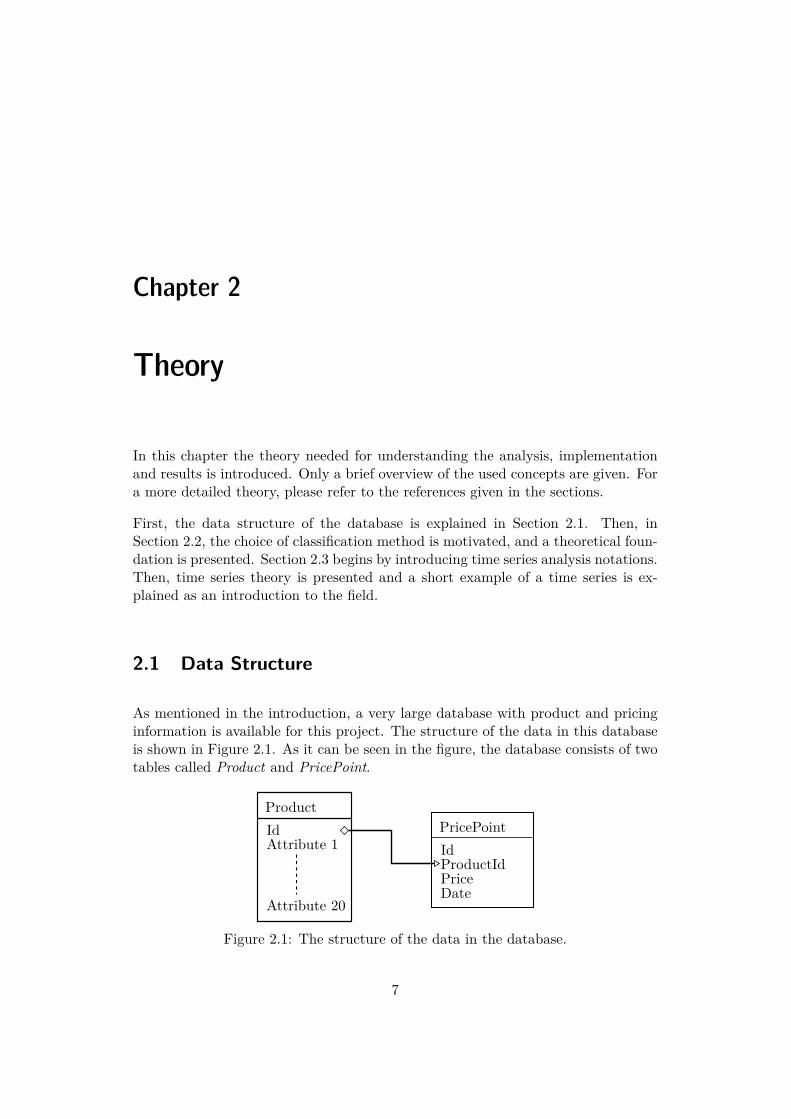
As mentioned in the introduction, a very large database with product and pricinginformation is available for this project. The structure of the data in this databaseis shown in Figure 2.1. As it can be seen in the figure, the database consists of twotables called Product and PricePoint.
ProductIdAttribute 1
Attribute 20
PricePointIdProductIdPriceDate
Figure 2.1: The structure of the data in the database.
7

CHAPTER 2. THEORY
A table in a database is a method to define the structure of the data stored in it.All the products stored in the database have the format of the Product table and allthe price points have the format of the PricePoint table. The Id field, which bothtables have, is a unique identifier for an entry in the database. This means thateach time that a new product or price point is submitted to the database, it getsan Id that no other product has or will have, and keeps this Id as long as it is inthe database. This particular database is of a type called a relational database [11].A relational database enables relations between the tables. In Figure 2.1, one suchrelation is defined by the arrow between the Product’s Id (PK - private key) andthe PricePoint’s ProductId (FK - foreign key). The relation is of the type one tomany, which means that one Product can have a relation with many PricePoints.The foreign key field in the PricePoint table connects it to a specific product in sucha way that the foreign key is the same as the private key of one product entry. Inthis way one product can have many price points and each price point is connectedonly to one product.
An example of a couple of entries in the database is shown in Table 2.1. In theexample, there are two product entries. Each entry has a unique Id and someattributes which can be unique, but most often are not. There are four price pointentries, each with a unique Id. However, all price points from Id 1 to 3 have thesame ProductId. This is the relation that tells that all these price points belongto the same product, namely the one with Id 1. The reason for this structure isthat each product can have many price points and each price point corresponds tothe price at a specific time. In this example the product with Id 1 has three pricepoints for three different dates, while the product with Id 2 only has one price pointcorresponding to one date.
ProductId Attribute 1 Attribute 21 A 152 B 15
PricePointId ProductId Price Date1 1 2000 2014-06-242 1 2000 2014-06-253 1 1900 2014-06-264 2 3000 2014-06-26
Table 2.1: Example of a couple of entries in the database.
The fields of the tables Product and PricePoint in the database have a number ofdifferent data types. Table 2.2 lists these datatypes and gives a short commenton each one. The different kinds of data types set limitations on what sorts ofclassification algorithms can be used, which is discussed in Section 2.2.1.
8

2.2. CLASSIFICATION
Data Type Commentsint Integer value, whole numbers.float Floating-point value, decimal numbers.bit Boolean value, 0 or 1, true or false.varchar Variable character field, strings of text.date A date with year, month, day, hour and so on.
Table 2.2: Data types in the database.
2.2 Classification
The problem of classification is that of assigning classes to objects of unknown class.The set of possible classes is discrete in contrast to the case in parameter estimation.In the field of machine learning the problem can be further divided into unsupervisedand supervised learning [4].
In unsupervised learning there is no prior information about which object shouldbelong to which class. Sometimes not even the set or number of possible classesis known. It is entirely up to the classification algorithm to group similar objectstogether. Figure 2.2 shows an example of unsupervised learning, where a couple ofobjects are classified according to their geometrical similarity.
Objects without class
Classification algorithm?
? ?
Objects with assigned class
C1
C2 C3
Figure 2.2: Unsupervised learning.
In supervised learning there exists a training set of objects, where the class is alreadyknown. This set of objects is called the training data. In this case the aim is toclassify the rest of the given objects by looking at their attributes and comparingto the objects with an already known class. An example of supervised learning isshown in Figure 2.3, where the classification algorithm uses the training data toclassify the geometrical shapes in the predefined classes.
There are many different classification algorithms and, as explained in Section 2.2.1,the Decision Tree Classification approach was chosen for this project. Section 2.2.2provides the theory on how to do classification when one already has a tree andSection 2.2.3 explains how to build a decision tree from training data.
9

CHAPTER 2. THEORY
Objects without class
Classification algorithm
?
? ?
Objects with assigned class
Training data
T
S C
T
S C
Figure 2.3: Supervised learning.
2.2.1 Choice of Method
There is a wide range of classification algorithms suitable for different kinds ofclassification problems. Table 2.3 holds an overview of some common classificationalgorithms and their characteristics. As discussed in Section 1.2.1, there are severalrequirements on the classification algorithm. The most important requirements arethat it should be fast enough to work in real time and also that the employeesshould find the result satisfactory.
A technical constraint stems from the fact that the available data has a predefinedset of data types (as explained in Section 2.1). These data types are both of con-tinuous and discrete nature, and some are also categorical. A categorical variablehas the property that it can only adopt a fixed set of values. These values may nothave a measure of length, meaning that for instance size comparison between twovariables is not possible. As an example of this, consider the integer numbers andcompare with types of weather. We all know that 5 is larger than 3 and smaller than6 and we can also define a distance between the two integers i1 and i2 as d = |i1−i2|.On the other hand, we cannot say that rainy weather is larger than sunny weatheror define a distance between the two (of course we can, but it would not make muchsense). Table 2.4 holds a description of the different data type properties.
The existing data types in the database set the requirement of our classificationmethod that it has to be able to handle both categorical and non-categorical pre-dictors. This rules out the classification methods “Support Vector Machines” and“Discriminant Analysis” as suitable algorithms. “Naive Bayes” is not suitable ei-ther, because of the fact that it is only fast for small datasets and the dataset fromthe database is very large. That leaves “Decision Trees” and “Nearest Neighbour”
10

2.2. CLASSIFICATION
Algorithm FittingSpeed
PredictionSpeed
MemoryUsage
Easy toInterpret
CategoricalPredictors
PredictiveAccuracy
DecisionTrees
Fast Fast Low Yes Yes Low
SupportVectorMachines
Medium Medium Lowfor fewsupportvectors
Easyfor fewsupportvectors
No High
NaiveBayes
Fast forsmalldatasets
Fast forsmalldatasets
Low forsmalldatasets
Yes Yes Low
NearestNeighbour
Fast Fast High No Yes Good in lowdimensions
DiscriminantAnalysis
Fast Fast Low Yes No Good whenmodellingassumptionsare satisfied
Table 2.3: Overview of classification algorithms [14, 20].
Type Description ExampleContinuous A continuous variable (de-
fined distance)1.0, 1.2, 1.5
Discrete A discrete variable (defineddistance)
1, 2, 3
Categorical Distinct and separate values(no defined distance)
Sunny, rainy and cloudyweather
Table 2.4: Description of data type properties.
as good alternatives as they are both fast and handle categorical predictors. Thereare two main differences between them which are that “Nearest Neighbour” has ahigh memory usage and is not easy to interpret while “Decision Trees” has a lowmemory usage and is easy to interpret. One of the requirements of the algorithm(from Section 1.2.1) is that it should give results that are easy to interpret, whichmakes the “Decision Tree” algorithm the best one for the given task. It is fast forfitting and prediction, handles categorical predictors, has a low memory usage andis easy to interpret. The only drawback is that it has relatively low predictive accu-racy compared to the other algorithms. However, the requirement is that it shouldclassify the data in a satisfactory way according to the employees. In the results inSection 4.1.4 it is shown that this actually is fulfilled.
With the motivation above, decision trees are chosen for the classification of the data
11

CHAPTER 2. THEORY
in this project. Some decision tree algorithms are presented in Table 2.5. Because ofthe large amount of information and intuitive design of the ID3 algorithm, this wasthe first algorithm considered. One very important limitation of the ID3 algorithm isthat it does not handle discrete attributes [33], which is needed for the classificationin this project. However, the C4.5 algorithm improves on this point [32] and it isalso able to handle missing attribute values. Therefore, the C4.5 algorithm waschosen for the project.
Algorithm CommentID3 Iterative Dichotomiser 3C4.5 Successor of ID3CART Classification And Regression TreeCHAID CHi-squared Automatic Interaction Detector
Table 2.5: Decision tree algorithms.
2.2.2 Classifying With an Existing Decision Tree
A decision tree can be seen as a graph representation of a decision algorithm whereeach node holds a statement that is either true or false. From each node there aretwo directed edges where one correspond to true, and one to false. Depending onthe value of the statement, the decision algorithm continues along the correspondingedge. The first node, where the decision algorithm starts, is called the root node andthe last nodes, where no further decision can be made, are called leaf nodes.
A decision tree is used when classifying objects of unknown class. The decisionalgorithm starts at the root node and checks if this first statement is true or falsefor the object by checking its properties. Then, it continues until it reaches a leafnode. All leaf nodes have classes assigned, and this is the class that the algorithmassigns to the object.
An example of this process is shown in Figure 2.4. Consider you have an unknowngeometrical shape and you want to determine if it is a red equilateral triangle, anequilateral triangle, a hexagon or something else. Then you can start at the rootnode checking if the statement “Does it have three sides of equal length?” is true.Continuing down in the tree you will reach one of the leaf nodes and be able todecide which class it belongs to. This procedure have to be repeated for each objectthat should be classified. However, this classification method requires an existingdecision tree well built for the problem. The next section explains how to buildsuch decision trees.
12

2.2. CLASSIFICATION
Does it havethree sides ofequal length?
Is it red?Does it havesix sides of
equal length?
Equilateraltriangle Hexagon
Redequilateraltriangle
Unknown
true
truetruefalse
false
false
Figure 2.4: Decision tree example.
2.2.3 Building a Decision Tree
As explained in Section 2.2.1, the algorithm called C4.5 [32] was chosen for thisproject. C4.5 uses a simple and elegant method with the concept of “divide andconquer” for building decision trees. The general idea of the algorithm is presentedin Algorithm 1.
Algorithm 1: General algorithm for building decision trees [16].Data: training dataResult: a decision treecheck for base cases;let a′ be the attribute to split on;forall the attributes a do
calculate measure g(a) for how good a splits the training data;if g(a) better than g(a′) then
set a as new a′;end
endcreate a decision node that splits on a′;add the resulting data to the children of the node;recursively enter the children to the algorithm;
Let the training data set for the algorithm be denoted by D and the classes by{C1, C2, · · · , Cn}. In the example in Figure 2.3 the training data D would be theset of the triangle with class T, the square with class S and the circle with classC and the corresponding classes would be {T, S,C}. There are three base cases to
13

CHAPTER 2. THEORY
consider [32]:
1. The training data in D belong to the same class Ci. Then the decisiontree for D simply is a single leaf with this class. For example: If there areonly triangles labelled T in the training data D, there is no reason to build adecision tree, all data can be considered to belong to class T .
2. There is no training data in D. Then the resulting tree is a single leafwith the most frequent class in all the training data at the levels above in thedecision tree.
3. The training data in D belong to different classes. This is the mostinteresting base case where a decision tree has to be built to be able to dividethe tree for useful classification. In this base case a test is created (explainedlater), which divides the training data into two new sets depending on theoutcome of the test. Each of these training data sets are then recursivelyentered into the algorithm again and further divided until they reach one ofthe above base cases (refer to Algorithm 1). For example: If there is onetriangle labelled T and one square labelled S in the test data D, a test isneeded to tell the two apart. A good test in this case would be to consider thenumber of edges of each object. The test “Does the object have more than3 edges?” would divide the training data into two more test data sets whichboth would reach a case in the next recursion of the algorithm.
This recursive algorithm will first consider the whole training data set D and splitit until each subset of it reaches one of the first two cases. One important part tounderstand is how the test in base case number 3 is created. In the older algorithmID3 [33], this is performed with a statistic called the gain criterion G(X) [32]. Letf(Ci, D) be the number of cases in the training data D that belong to the classCi, |D| be the number of training cases in D, and X be a test under consideration.Then G is defined as
G(X) := I(D)− IX(D), (2.1)
where
I(D) := −k∑
i=1
f(Ci, D)|D|
log2f(Ci, D)|D|
, (2.2)
and
IX(D) :=n∑
i=1
|Di||D|
I(Di). (2.3)
14

2.2. CLASSIFICATION
f(Ci,D)|D| can be seen as the probability of randomly picking the class Ci from the
training data D. Then, by using Shannon’s general formula for uncertainty [37] weobtain the entropy I(D) in equation (2.2). IX(D) is another entropy measure afterthe training data D has been tested with the test X and got n outcomes of newtraining data Di. ID3 then selects the test that maximizes the gain criterion G inequation (2.1).
However, this approach favours tests that split the training data into many outcomeswhich can give an overfitted model [32]. In C4.5, this problem is overcome by insteadmaximizing the gain ratio criterion:
Gr(X) := G(X)A(X) , (2.4)
where
A(X) := −n∑
i=1
|Di||D|
log2|Di||D|
. (2.5)
A(X) acts as a normalizer that penalizes tests with many outcomes to balance thegain criterion. The next examples give an intuitive explanation of the measures(2.1) and (2.4).
Example 2.2.1 (Entropy). Entropy can intuitively be seen as the amount of in-formation in a distribution. A more general way of writing equation (2.2) is
I(D) = −k∑
j=1pj log2 pj (2.6)
where pj is the probability for the outcome j of the random variable D. Considerthe following three tosses of a coin, with different probabilities for heads and tailscoming up:
1. A fair coin. For a fair coin the probability of getting heads up and gettingtails up is equal (p(heads) = p(tails) = 0.5). In this case the entropy isI(D) = 1 according to Equation (2.6). To simplify the notation we writeI(0.5, 0.5) = 1.
2. A non-fair coin. For a coin that is not fair, the probability of getting headsup and getting tails up is not equal. If for example the probability for headsup is p(heads) = 0.8, the entropy is I(0.8, 0.2) = 0.72.
3. A coin with two equal sides. If the coin has heads on both sides, theprobability of heads is p(heads) = 1 and the entropy is I(1, 0) = 0.
15

CHAPTER 2. THEORY
In the first case, where the coin is fair, we know nothing about if the outcomewill be heads or tails up from a coin flip before the result is observed. After thecoin is tossed, we gain a lot of information of the outcome (from having no ideaof the outcome to know exactly) and therefore the information contained in thisdistribution is high. In contrast, in the third case where the coin has two equalsides, there is no information in the distribution at all. This is because we alreadyknow the outcome of the coin flip before it is carried out. After the coin is tossedand we observe the result, the knowledge of the outcome has not increased. In thecase of a non-fair coin, we know something about the outcome and the entropy istherefore somewhere between the entropy of the fair coin and the coin with twoequal sides. Figure 2.5 shows the entropy as a function of the probability p(heads)to get heads up for a coin.
0.0 0.2 0.4 0.6 0.8 1.0
0.0
0.2
0.4
0.6
0.8
1.0
p(heads)
Entro
py
Figure 2.5: Entropy as a function of the probability of heads for a coin toss.
IX(D) and A(X) are similar entropy measures as the entropy I(D) in the previousexample. IX(D) sums the weighted information contained in all the new partitionsDi, i = 1, . . . , n , resulting from a specific split X from the training cases D.The information gain G(X) is then the difference of the current information of thedistribution and the information after the split. We want the information remainingin the distribution as low as possible after the split, because it means that we havemore knowledge of the outcome (compare to the coin flip where the coin has twoequal sides). Therefore, the information gain G(X) should be maximized for a goodsplit.
To get the gain ratio criterion Gr(X) for a split, the normalizer A(X) is used tonormalize the gain criterion. A(X) is larger for splits with many partitions Di than
16

2.2. CLASSIFICATION
for few partitions. To see this, consider the extreme case for a split X0 which doesnot split D. Then |Di|
|D| = 1 and A(X0) = 0. This makes Gr(X0) large. The otherextreme is X∞ which results in an infinite number of splits. Then A(X∞) is largeand Gr(X∞) is small. In reality the splits are somewhere in between and A(X)acts as a normalizer that penalizes many splits Di, as previously mentioned. Ex-ample 2.2.2 illustrates these concepts with some training data.
Example 2.2.2 (C4.5). This example illustrates some concepts from the C4.5algorithm by considering the training data in Table 2.6. In the table, the attributes“Weather”, “Have ice cream”, “Have money” and “Age” are shown together withthe decision if an ice cream should be eaten or not.
Weather Have ice cream Have money Age Eat ice cream?Hot Yes Yes Old EatHot Yes Yes Young EatHot Yes No Old EatHot Yes No Young EatHot No Yes Old EatHot No Yes Young EatHot No No Old Don’t eatHot No No Young Don’t eatCold Yes Yes Old Don’t eatCold Yes Yes Young Don’t eatCold Yes No Old Don’t eatCold Yes No Young Don’t eatCold No Yes Old Don’t eatCold No Yes Young Don’t eatCold No No Old Don’t eatCold No No Young Don’t eat
Table 2.6: C4.5 example training data.
From equation (2.2) we get
I(D) = I
( 616 ,
1016
)= − 6
16 log2616 −
1016 log2
1016 = 0.95, (2.7)
which is the entropy of the distribution. If we consider a split on “Weather”, we get
IWeather(D) = 816I
(68 ,
28
)+ 8
16I(8
8 ,08
)= 8
16 · 0.81 + 816 · 0 = 0.41 (2.8)
from equation (2.3), and G(Weather) = 0.54 from equation (2.1). The results fromthe other attributes are shown in Table 2.7. In this table, one can see that the
17

CHAPTER 2. THEORY
information gain is largest for “Weather”, equal for “Have ice cream” and “Havemoney”, and 0 for “Age”. Therefore, the split is done on the attribute “Weather”in this simple example.
Split Attribute I(D) IX(D) G(X)Weather 0.95 0.41 0.54Have ice cream 0.95 0.91 0.04Have money 0.95 0.91 0.04Age 0.95 0.95 0
Table 2.7: C4.5 example measures.
The decision tree from which the training data was generated can be seen in Fig-ure 2.6. In that tree, the attribute “Age” does not exist, i.e. the attribute does notaffect the outcome if we should eat ice cream or not. This is reflected in Table 2.7where “Age” has the information gain G(Age) = 0. One can also observe that theattribute “Weather” is at the root of the tree and that if it is “Cold” we shouldnever eat ice cream. In this sense, it is a good split variable which is reflected in itsrelatively high information gain.
Weather?
Have icecream?
Don’t eatHave money?Eat
Hot
YesNo
Cold
Yes No
Figure 2.6: C4.5 example decision tree.
2.3 Time Series Analysis
There are many methods for predicting future values based on previous observations.Methods that have been considered for this thesis are artificial neural networks [42],
18

2.3. TIME SERIES ANALYSIS
support vector machines [10], time series analysis [8, 18] and hidden Markov mod-els [7]. Due to the limited amount of time for the thesis, not all methods could betested on the data set. Time series analysis was chosen for further analysis becauseof the following reasons:
• Time series analysis is well known and used for many applications.
• There are many available tools for working with time series analysis.
• The available dataset is typical for time series analysis.
The fact that time series analysis is well known and used has led to large amountsof information available in the area. There are several papers and books writtenon the subject [18, 8] and software such as Matlab, R [34] and R.NET [35] haveimplementations that enable fast testing on the real data set. The other methodsconsidered does not seem to have equally strong standardizations of the theoreticalapproach. Statements such as “While artificial neural networks provide a great dealof promise, they also embody much uncertainty” [42] and “To overcome the chal-lenges in predicting time series with hidden Markov models some hybrid approacheshave been applied” [7] are common when reading about the other methods. Thisgives the impression that they are not equally developed and time series analysis isa more robust choice in this sense.
2.3.1 Introduction
A time series {Xt} is a collection of observations at different points in time, usuallyequally spaced. Time series analysis is the study of previously collected time seriesdata with the hope that it could say something about the future outcome of theobserved object.
In this section some important concepts from time series analysis needed for theunderstanding of the analysis, implementation and results, are introduced.
Stationarity
Stationarity is an important concept in time series analysis. First, the mean andcovariance functions are introduced:
Definition 2.3.1 (Mean and Covariance). For a time series {Xt}, themean functionµX(t) is defined as
µX(t) = E[Xt], (2.9)
and the covariance function γX(r, s) as
19

CHAPTER 2. THEORY
γX(r, s) = Cov(Xr, Xs) = E[(Xr − µX(r))(Xs − µX(s))]. (2.10)
Stationarity is then defined as:
Definition 2.3.2 (Stationarity). A time series {Xt} is weakly stationary if [8]:
(i) µX(t) = µ, ∀t ∈ Z,(ii) γX(t+ h, t) = γX(h), ∀h, t ∈ Z.
(2.11)
Stationarity implies that the mean and autocovariance function of the time seriesdo not change with time, making it possible to build time independent models forfuture behaviour of the time series. If the process considered is not stationary, itis first transformed to obtain these properties, please refer to Example 2.3.1 fordetails.
White Noise
When constructing time series models, white noise is an important building block.It is defined by:
Definition 2.3.3 (White noise). A process {Zt} is white noise if [8]
(i) E[Zt] = 0,(ii) E[Z2
t ] = σ2 (2.12)
and {Zt} is a sequence of uncorrelated random variables. If {Zt} is white noise withmean 0 and variance σ2, it is written {Zt} ∼WN(0, σ2).
ACF and PACF
The autocovariance function and partial autocovariance function are important toolswhen working with time series data. If the time series {Xt} is stationary, the timeindependent covariance function can be simplified:
Definition 2.3.4 (Autocovariance/autocorrelation function). If {Xt} is a station-ary time series, the autocovariance function ACVF, γX(h) is defined as [8]
γX(h) := γX(t+ h, t), (2.13)
20

2.3. TIME SERIES ANALYSIS
and the autocorrelation function ACF, ρX(h) as
ρX(h) := γX(h)γX(0) . (2.14)
The partial autocorrelation function is then defined by:
Definition 2.3.5 (Partial autocorrelation function). If {Xt} is a stationary timeseries, the partial autocorrelation function PACF, αX(h) is defined as [8]
(i) αX(0) := 1,(ii) αX(1) := ρX(1),(iii) αX(h) := ρX(Xh+1 − PX2,...,Xh
Xh+1, X1 − PX2,...,XhX1), h ≥ 2,
(2.15)
where PX2,...,XhXn is the best linear predictor of Xn given X2, . . . , Xh.
The sample versions, which can be calculated from real time series data, are
γX(h) = 1n
n−|h|∑t=1
(xt+|h| − x)(xt − x), −n < h < n, (2.16)
ρX(h) = γX(h)γX(0) , (2.17)
and
αX(0) = 1,αX(1) = ρ(1),αX(h) = ρ(Xh+1 − PX2,...,Xh
Xh+1, X1 − PX2,...,XhX1), h ≥ 2.
(2.18)
One important reason why they are good tools for time series analysis is that theyhave the properties that ρ(h) = 0 if h > p for AR(p) models and α(h) = 0 if h > qfor MA(q) models. Thus, they can be used for finding the order of those modelsfrom time series data by inspecting their sample autocorrelation functions. Theyare also useful for deciding if a time series is white noise or not. This is done byconsidering the bounds ±1.96√
nwhere n is the number of observations. If more than
95 % of the values of the ACF ρX(h) for h 6= 0 fall within these bounds, {Xt} canbe considered white noise and no further modelling is possible [9].
21

CHAPTER 2. THEORY
Models
There are a couple of standard models for time series analysis and in this projectthe vector autoregressive (VAR) model was chosen for further analysis (the reasonfor this is explained in the end of this section). To give an understanding of themodel, a couple of simpler models are first introduced [8].
AR(p) An AR(p) model is one of the simplest models for a weakly stationaryprocess. In this model the future values of {Xt} depends on the p previous valuesand the current noise realization:
Xt − φ1Xt−1 − . . .− φpXt−p = Zt, Zt ∼WN(0, σ2). (2.19)
MA(q) A MA(q) model is similar to the AR model, but instead of depending onprevious values of {Xt} it depends on q previous values of the noise term:
Xt = Zt + θ1Zt−1 + . . .+ θqZt−q, Zt ∼WN(0, σ2). (2.20)
ARMA(p,q) An ARMA(p,q) model is a combination of an AR(p) model anda MA(q) model; it depends both on previous values of {Xt} and of the noise{Zt}:
Xt−φ1Xt−1− . . .−φpXt−p = Zt +θ1Zt−1 + . . .+θqZt−q, Zt ∼WN(0, σ2). (2.21)
VAR(p) The VAR(p) model used for the implementation in this project is amultivariate version of the previously described AR model with structure
Xt = ν + A1Xt−1 + . . .+ ApXt−p + Ut, (2.22)
where Xt = (X1,t, . . . , Xn,t)>, ν is a n × 1 vector holding model constants, Ai aren × n square matrices with model parameters, E[UtU>t ] = Σ, E[UtU>t−k] = 0 fork 6= 0, and Σ is a positive definite covariance matrix [18, 31]. All VAR(p) modelscan be rewritten as a VAR(1) model with the notation [18]
X = BZ + U, (2.23)
where
22

2.3. TIME SERIES ANALYSIS
X := [X1, . . . ,Xt],B := [ν,A1, . . . ,At],Zt := [1,Xt, . . . ,Xt−p+1]>,Z := [Z0, . . . ,Zt−1],U := [U1, . . . ,Ut].
(2.24)
There are many other more complex models within time series analysis [18]. Exam-ples are vector autoregressive moving average (VARMA), autoregressive conditionalheteroskedasticity (ARCH), generalized autoregressive conditional heteroskedastic-ity (GARCH), nonlinear generalized autoregressive conditional heteroskedasticity(MGARCH) among others. VAR models are the only considered models for thisthesis because of their simplicity and that they give good results for the availabledata set. If they would not have been sufficient for the task and time allowed, morecomplex models would have to be tested. However, as it can be seen in the resultsin Section 4.2, the VAR models give good predictive accuracy.
AIC
AIC is short for Akaike’s information criterion and is a very useful measure fordeciding which model to use. It is defined as [3, 17]:
VAIC = 2θ − 2 log(L) (2.25)
where θ is the number of model parameters and L is the maximum value of themodel’s likelihood function for a given data set. The model structure that minimizesthe AIC is often a good choice of model, since it has a good balance between fewparameters (low value of θ) and a good representation of the data (high value ofL).
Model Estimation
By using the general VAR(1) model from equation (2.23), the estimated modelparameters B can be derived to be [18]:
B = XZ>(ZZ>)−1 (2.26)
As seen in the equation, estimation can be carried out by only considering the pastobservations of the variables contained in X and Z.
23

CHAPTER 2. THEORY
Prediction
The best linear predictor Y of Y in terms of X1, X2, . . . , Xn is [12]:
Y = a0 + a1X1 + . . .+ anXn, (2.27)
with constants a0, a1, . . . , an chosen such that the mean square error E[(Y − Y )2]is minimized. The predictor is determined by
Cov(Y − Y,Xi) = 0, i = 1, . . . , n. (2.28)
In the case of the VAR processes (equation (2.22)) used in this project, the bestlinear predictor fulfilling this requirement is [18]
Xt = A1Xt−1 + . . .+ ApXt−p (2.29)
This is intuitive to understand, since the best predictor is the same as our modelwith estimated parameters and with the noise term disregarded.
Granger Causality
The Granger causality test is a good tool for determining which time series couldbe useful for prediction of other time series [13]. One possible approach to defineGranger Causality is the following [38]:
Definition 2.3.6 (Granger Causality). Let F = {Xt, Yt, Xt−1, Yt−1, . . . , X1, Y1}where {Xt} and {Yt} are time series. Then, if the variance of Yt+h based on F issmaller than the variance of Yt+h based on {Yt, Yt−1, . . .} for any positive lag h, Xt
is Granger causal for Yt with relation to F .
In the case of VAR(1) models with only two variables a test for this causality issimple to perform. If the VAR model from equation (2.22) is written as
Xt =[X1,t
X2,t
]=[α11 α12α21 α22
] [X1,t−1X2,t−1
]+ Ut, (2.30)
the Granger test can be performed by looking at the α values. The null hypothesisthat X1,t does not Granger cause X2,t is then true if α21 = 0 [39].
When testing models with K > 2 variables, Xt is split in the two parts
24

2.3. TIME SERIES ANALYSIS
Xt =[X1,t
X2,t
], (2.31)
such that X1,t has K1 variables, X2,t has K2 variables and K1 + K2 = K. Then,the VAR(p) can then be rewritten as [18, 31]:
[X1,t
X2,t
]=
p∑i=1
[α′11,i α′12,i
α′21,i α′22,i
] [X1,t
X2,t
]+ Ut. (2.32)
The null hypothesis that X1,t does not Granger cause X2,t is in this case definedas [31]
α′21,i = 0 ∀i = 1, 2, . . . , p. (2.33)
Therefore, we test if there exists any α′21,i 6= 0 for i = 1, 2, . . . , p. This statistic hasthe F-distribution F (pK1K2, nK − p) [18], which is used in later analysis.
2.3.2 A Classic Approach
A classic method [8] for time series analysis is as follows:
1. Find the main features of the time series such as trends, seasonal componentsand outliers.
2. Remove the trend and seasonal components to get a stationary, detrended anddeseasonalised time series.
3. Choose a model that fits the stationary time series.
4. Use the model for forecasting of the model residuals.
5. Add the previously removed trends and seasonal components to the predictionto get a forecast of the original data.
Consider the following example which illustrates the process:
Example 2.3.1. Figure 2.7 shows the average monthly atmospheric carbon dioxidelevels measured at Mauna Loa, Hawaii, since 1958. A polynomial trend is plottedin blue. There is also an evident yearly seasonal component, and another seasonalcomponent with a period of approximately 30 years. Figure 2.8 shows the datawhen the trend and the two seasonal components are removed. This data is usedto build an AR(9) model and the sample autocorrelation of the residuals for one-step prediction of this model is shown in Figure 2.9. The sample autocorrelation ofthe residuals from the model resembles white noise, which means that no further
25

CHAPTER 2. THEORY
time series models are possible with this approach. The AR model is then used toforecast the residuals, and then the trend and seasons are added to get the forecastresult in Figure 2.10.
1960 1970 1980 1990 2000 2010
320
340
360
380
400
Time
CO
2[ppm
]
1960 1970 1980 1990 2000 2010
−1
0
1
2
Time
CO
2[ppm
]Figure 2.7: Original data and trend. Figure 2.8: Data without trend and
seasonal components.
0 5 10 15 20−0.10
−0.05
0.00
0.05
0.10
Samples1960 1970 1980 1990 2000 2010 2020
320
340
360
380
400
Time
CO
2[ppm
]
Figure 2.9: Autocorrelation of residu-als for an AR(9) model.
Figure 2.10: Forecast.
26

Chapter 3
Analysis and Implementation
In this chapter an analysis of the problem defined in Section 1.2 is presented. Theimplementation of the solution is also explained. The implemetation tools are firstdescribed in Section 3.1. Then, in Section 3.2, the classification part is detailed andthe time series analysis can be found in Section 3.3.
Figure 3.1 gives an overview of the implementation and its three sub parts. Theuser interacts with a front end, which in turn handles the information flow to theclassification and times series algorithms, as well as interacting directly with thedatabase. Among other things, the user can display pricing data in raw numbersand in graphs. He can also enter classes manually or automatically with help fromthe classification algorithm. The time series analysis is used when the user requestsa prediction of a specific class in the database.
User
Classification
Time Series Analysis
Database
Implementation
Front End
Figure 3.1: Implementation overview.
3.1 Implementation Tools
At the company as well as at many other workplaces the operating system in useis one of the systems from the Microsoft® Windows family. The database withproduct and price information described in Section 2.1 is of the type Microsoft®SQL Server [23]. There are many programming languages to choose from that
27

CHAPTER 3. ANALYSIS AND IMPLEMENTATION
would be suitable for the implementation, but since the users and the databaseonly use Microsoft® products, the programming language C# [25] was chosen. C#has many similarities with C, C++, Java and other object oriented programminglanguages. Microsoft® Visual Studio [26] was chosen as integrated developmentenvironment (IDE) because of its tight integration with C#, its excellent debuggingand performance tools and also the simplicity of working with databases within theprogram. To have good control of the source code Microsoft® Team FoundationServer [24] was configured and installed on an external server. It was used both forwork tracking and source control.
3.2 Classification
To reuse existing code for the C4.5 classification algorithm the scientific computingframework Accord.NET [2] was used. The full source code of the framework is avail-able and the implementation of the C4.5 algorithm is also public [1]. The availablecode is a direct implementation of the algorithm described in Section 2.2.3.
The integration of the C4.5 algorithm consists of the following parts:
1. A method for creating a decision tree from a selection of products.
2. A method for storing a decision tree in the database.
3. A method for classifying a selection of products with a decision tree.
Each of these parts are explained in more detail below.
3.2.1 Creating a Decision Tree
As explained in Section 2.2, a set of training data is needed to build a decision treethat can be used for classifying other data. The data that needs to be classified iseach product in the database with attributes of the data types shown in Table 2.2 onpage 9. The idea of creating this decision tree is to simplify the classification workof the employees. The training data for building the tree is a couple of products ineach class, which the employee has manually labelled.
In Algorithm 2, a high level overview of the implementation is shown. In the realimplementation there are many help methods and data conversion algorithms used,but they are not relevant for understanding the structure. The algorithm startsby retrieving a list of product ids and a corresponding class to every id. This listhas been created by an employee who has picked out a collection of products andmanually labelled them in the front end application. The algorithm then gets allthe products from the database from the list of ids and sets the corresponding classof each product.
28

3.2. CLASSIFICATION
Algorithm 2: Creating a decision tree.Data: list of product ids and list of manually set classesResult: a decision treedatabase products ← all products from the database with id from input list;set the class of all database products from input classes;set the flag ’manually classified’ on all database products;update database;codebook ← created codebook from all database products;decision attributes ← set decision attributes to consider;input ← all decision attributes from all database products;output ← all manually set classes from all database products;decision tree ← decision tree generated from input and output;
Each product in the database also has a boolean field called manually classifiedwhich is set to true for all the selected products. The purpose of this field is to notreclassify these products later on when the classification described in Section 3.2.3takes place and also to label them as training data. This reclassification couldotherwise happen if an employee for instance classified a single product in a classwith products with very different attributes. In the creation of the decision treethis product would be considered an outlier and then it could get another classwhen classifying it at another instance. By labelling it as manually classified andignoring it in further classification, this unwanted behaviour is avoided. When thedatabase products are updated with a class and label, the changes are submittedto the database.
The implementation of the C4.5 algorithm used is not able to handle other thaninteger and float values. Integer values represent both discrete and categorical pre-dictors (distinguished with a flag in the code), and float values represent continuouspredictors. A codebook [2] is used to convert the other data types, for instancestrings of text and boolean values. The principle of the codebook is very simpleand shown in Figure 3.2. To the left in the figure, attributes with values that arenot integers are shown. A codebook is created where each unique attribute valueis assigned an integer code. The codebook is then used to change the attributes tointegers so that they can be used in the algorithm. The same codebook is neededlater in the implementation (refer to Section 3.2.3) to translate the integer codesback to their original values.
Decision attributes are the attributes of the products that the algorithm will con-sider when building the decision tree. Some attributes may be known to have noimpact on which class the product belongs to. Examples of such attributes are theId (as each product has a unique Id) and the previously mentioned flag that theclass is manually assigned.
The input values are then all the chosen decision attributes from all the databaseproducts. The output values are the manually assigned classes that are given from
29

CHAPTER 3. ANALYSIS AND IMPLEMENTATION
Attributes
A1A2A3A4
Value
ABCA
Value
ABC
Code012
Attributes
A1A2A3A4
Value0120
Codebook
Figure 3.2: Codebook example.
the parameter of the method. The input and the output values are then entered inthe C4.5 algorithm which builds and returns a decision tree object.
3.2.2 Storing a Decision Tree
When new products are submitted to the database there is a need of automaticallyassigning them a class in the back end application. It would be very time consumingto rebuild the tree each time a new product should be classified, as many newproducts are added continuously. This gives rise to the need for storing the tree so itis easily accessible from multiple applications running on different computers.
Since a Microsoft® SQL Server database is already available a new table is added inorder to store the trees. The simple design of this table is shown in Figure 3.3. It hasan id field, which is unique for each entry, and two binary fields. The binary fieldscan store binary data with a specified length of bytes, i.e. a binary file. The firstbinary field is for storing the actual tree and the second to store the correspondingcodebook. To be able to store the tree and the codebook in the database, they arefirst serialized. Serialization is a way to convert objects in the program to binaryfiles [22]. The binary files are then stored in the database.
DecisionTreeIdBinary TreeBinary Codebook
Figure 3.3: Table to store decision trees in the database.
3.2.3 Classifying With a Decision Tree
When an employee has entered training data and a decision tree has been created(Section 3.2.1) and stored (Section 3.2.2) the next step is to use this tree to classify
30

3.3. TIME SERIES ANALYSIS
other products. An overview of the algorithm for classification of products is shownin Algorithm 3.
Algorithm 3: Classification of products.Data: list of ids of products to classifyResult: classified productsdatabase products ← all products from the database with id from input list;codebook ← gets codebook from the database with highest id;binary decision tree ← gets decision tree from the database with highest id;compiled decision tree ← compiles the binary decision tree;forall the database products p do
coded attributes ← converts p’s attributes with codebook;coded class ← enter coded attributes in compiled decision tree;class for p ← convert the coded class with codebook;
endupdate database;
The algorithm takes in a list of product ids of products to classify. The correspond-ing entries in the database (database products) are then retrieved. To be able toclassify these products the last codebook and decision tree are also fetched. Becauseof the high priority on the speed of the classification due to the large amount ofdata processed, the binary classification tree from the database is first serialized andthen compiled into executable code. Then each product’s arguments are convertedwith the codebook and then fed into the compiled decision tree. The tree outputsa coded class which is coded back with the codebook to get the right class. Whenall products are classified, the changes are submitted to the database.
3.3 Time Series Analysis
This section holds an analysis and a description of the implementation of the timeseries analysis. In the analysis part, an example is presented to introduce themethods used. Then, the same methods are used with real data from the database.The implementation part explains which programming tools were used and alsogives pseudo code for the algorithm.
3.3.1 Analysis
In this section an analysis of the structure of the available data is presented, moti-vating the implementation in Section 3.3.2. First, we consider a simplified exampleto get an insight in the methods used:
31

CHAPTER 3. ANALYSIS AND IMPLEMENTATION
Example 3.3.1. In Figure 3.4 the price evolution of three example products isconsidered for approximately 40 days. These three products have the exact sameprice evolution except that Product 2 is shifted one day in relation to Product 1,and Product 3 is shifted two days in relation to Product 1. One could say thatin this class of products, Product 1 is the market leader and sets the price thatthe other products are following. This is a behaviour that is frequent in real data.However, in real data it has much higher complexity in the sense that there couldbe more than one market leader in a class, the products don’t follow each otherexactly one day after, etc.
6070
8090
Prod
uct1
6070
8090
Prod
uct2
6070
8090
0 10 20 30 40
Prod
uct3
Time
Three Products
Figure 3.4: Example price evolution for three products.
In Figure 3.5, the ACFs for the differentiated price evolutions of the example prod-ucts are shown. The three diagonal sub plots are the sample autocorrelation withthe product itself, and the other sub plots are the sample crosscorrelation betweeneach two of the products. Notice how the three diagonal plots satisfy the hypothesisof white noise sequences discussed in Section 2.3. This essentially tells us that theprice evolution for each product when considered separately seems random and itis not possible to build a model that predicts the future price evolution in a reliableway. The best that can be done in this case with the presented theory is to estimatethe trend and stop there. However, the interesting information is in the three subplots called Prd2 & Prd1, Prd3 & Prd1 and Prd3 & Prd2. Notice the single highpeak at lag −1, −2 and −1 in each plot respectively. This corresponds to thatProduct 2 is a 1-day delayed version of Product 1, Product 3 is a 2-day delayedversion of Product 1 and Product 3 is a 1-day delayed version of Product 2. Thisis not entirely a surprise, since it is exactly how the example was built. However,
32

3.3. TIME SERIES ANALYSIS
this means that it is possible to build a relevant VAR model of this time series.
0 2 4 6 8 10
-0.2
0.4
1.0
Lag
Product 1
0 2 4 6 8 10-0
.20.
41.
0Lag
Prd1 & Prd2
0 2 4 6 8 10
-0.2
0.4
1.0
Prd1 & Prd3
-10 -6 -4 -2 0
-0.2
0.4
1.0
Lag
Prd2 & Prd1
0 2 4 6 8 10
-0.2
0.4
1.0
Lag
Product2
0 2 4 6 8 10
-0.2
0.4
1.0
Lag
Prd2 & Prd3
-10 -6 -4 -2 0
-0.2
0.4
1.0
Lag
Prd3 & Prd1
-10 -6 -4 -2 0
-0.2
0.4
1.0
Lag
Prd3 & Prd2
0 2 4 6 8 10
-0.2
0.4
1.0
Lag
Product3
Lag
Figure 3.5: The ACF of the differentiated example products.
Figure 3.6 shows the result when making a prediction of each product from theestimated VAR model. The blue line is the best prediction and the red lines show95 % confidence bounds for the prediction. The forecast for Product 1 is simplythat it will follow the estimated trend and may also have some weak dependence onthe earlier behaviour. The forecast for Product 2 on the first forecasted day is thatthe price will go up exactly as it did for Product 1 the day before, which makes alot of sense. Notice how the confidence bounds follow the same behaviour as thebest prediction. This stems from the fact that Product 2 has always in the pastfollowed Product 1 exactly one day after. Therefore, according to our model, it willcontinue doing that. However, the prediction for days after the first one will havea higher uncertainty and be equal to the prediction for Product 1. The forecast forProduct 3 follows the same pattern where during the first two days it will first haveconstant price, then follow Product 1 and 2 in the price increase and then also havethe same prediction as Product 1 had the first day.
When working with real data the situation is more complex as mentioned previously,
33

CHAPTER 3. ANALYSIS AND IMPLEMENTATION
Forecas t of s eries Product1
0 10 20 30 40 50
5080
Forecas t of s eries Product2
0 10 20 30 40 50
5080
Forecas t of s eries Product3
0 10 20 30 40 50
6090
Figure 3.6: Prediction of the example products.
but it still follows the same idea as the idealized example. In the implementation allproducts are modelled with all other products in the same class, but for the analysisin this section the mean price in the class is chosen instead to limit the number ofplots. Figure 3.7 shows the price evolution for a product and the mean price in theclass the product belongs to. In the figure it can be seen that they follow each othera bit, which is a common behaviour also for products of the same class.
Figure 3.8 shows the ACF of the differentiated products and mean. By studyingthe figure one can see that, as in the simple example, the product and the mean bythemselves satisfy the white noise hypothesis and it is not possible to build modelswith good prediction capabilities using general time series analysis. The sub plotProduct & Mean shows lack of correlation, which gives the information that theproduct does not follow the mean price in the class. The interesting informationcan be gained in the sub plot Mean & Product where it can be seen that there issome correlation approximately for lags from −1 to −7. This means that the meanprice actually follows the product’s price and it is possible to build a VAR model forthis behaviour. In this example it is the mean price that follows the product’s price,but in the real implementation correlation is found between different products inthe same class. In this way one can see which products in the class are setting theprice and which products that follow others. Some products can also be completelyuncorrelated with all other products in the class and then the model will not givebetter predictions than simply estimating the trend.
34

3.3. TIME SERIES ANALYSIS
8000
8800
Prod
uct
7500
0 20 40 60 80 100 120
Mea
n
Time [Days]
Product and Mean
Figure 3.7: Price evolution for product and mean.
0 5 10 15
-0.2
0.4
1.0
Lag
ACF
Product
0 5 10 15
-0.2
0.4
1.0
Lag
Product & Mean
-15 -10 -5 0
-0.2
0.4
1.0
Lag
ACF
Mean & Product
0 5 10 15
-0.2
0.4
1.0
Lag
Mean
Figure 3.8: The ACF of the differentiated products and mean.
In Figure 3.9, the price prediction is shown for both the product and the mean,just after a change of the product’s price. As inferred by the earlier correlation,
35

CHAPTER 3. ANALYSIS AND IMPLEMENTATION
the prediction for the mean price is that it will also go down in the next couple ofdays, as it can be seen in the figure. However, the product’s price evolution is moredifficult to predict, since it is not correlated with previous values of itself or with themean price, as previously discussed. Therefore, the best prediction is mostly basedon the estimated trend and it has a relatively large confidence interval, implyingthat the prediction has low accuracy.
Forecas t of s eries Product
0 50 100 150
8000
Forecas t of s eries Mean
0 50 100 1506500
8500
Figure 3.9: Prediction of the product and mean.
3.3.2 Implementation
There are many software solutions for working with time series analysis. Matlaband R are both two popular alternatives. Since R is open software [34] and alsointegrates well with C#, it was chosen for this project’s implementation. Theintegration with C# is handled with the library R.NET [35]. This library enablesR code directly into the source of the project and also makes it simple to convertbetween different data types.
The time series algorithm implementation has a single yet difficult task: it shouldbe able to receive a number of products with their temporal pricing information,and for each product it should predict the future price evolution. An overview ofthe implementation is shown in Algorithm 4.
36

3.3. TIME SERIES ANALYSIS
Algorithm 4: Prediction of products.Data: list of products to predict and prediction lengthResult: list of products with predictionif prediction length larger than zero then
global first and last price point date ← 0;forall the database products p do
find the local first and last price point date for p;if any price point missing in between, linearly interpolate;
endglobal first price point ← last local first price point date;global last price point ← last local last price point date;start R engine with required packages;convert all product price point data to R format;build a univariate time series for each product;build a multivariate time series consisting of all products;create VAR model that minimizes AIC and considers trend;predict each univariate time series with the VAR model;convert prediction data back from R format and add to products;return products with prediction;
elsereturn products without prediction;
end
The purpose of the algorithm is that it should be able to receive a set of productswith corresponding price information and do a price prediction on each productaccording to the analysis in Section 3.3.1.
If the prediction length is larger than zero, meaning that a prediction should takeplace, it starts by going through all the products that should be predicted and findsthe first and the last recorded price for each product. For some of the productsthere is missing price information for a couple of dates between the first and lastpoints recorded. Then the price is linearly interpolated to get a full set of data.When all the individual first and last recorded price point dates have been found, aglobal first and last date are set. It is between these two dates that the time seriesmodel is built. Figure 3.10 shows the resulting time window for this method.
Then the R engine is started with R.NET [35] and the required packages are loaded.Since the database formats differ from the ones used by R.NET, some conversionstake place (they are not explained here due to space limitations). Then, the methodoutlined in Section 3.3.1 is implemented in R code. First, a univariate time seriesstructure is built for each product’s price points. Then, all these univariate modelsare put together into a single multivariate time series structure. From this mul-tivariate time series the VAR model that minimizes the AIC and also considerstrends is estimated according to the theory in Section 2.3. This model is then used
37

CHAPTER 3. ANALYSIS AND IMPLEMENTATION
Price
Time
Today
Time WindowFigure 3.10: Time window selection.
for prediction of each univariate time series. The prediction data is converted to asuitable format and then added to each product. Now the prediction is done andthe products are returned with the included predictions.
3.4 Front End
When working with C# the preferred framework for writing Graphical User In-terfaces (GUIs) is Windows Presentation Foundation (WPF) [27]. WPF uses theExtensible Application Markup Language (XAML) to structure design elements, ina similar way as HTML is used for websites. Instead of writing the XAML codemanually, Blend [21] was used for designing the GUI.
During the development of the front end, several meetings with the employees thatuse the GUI was held. During these meetings the current state of the program wasdisplayed and feedback was retrieved. It was an iterative process where several dif-ferent design approaches were implemented and tested between the meetings.
One important implementation detail is that each new action in the program, forinstance the creation of a decision tree, was started in a separate thread from theGUI, so that the interface always stayed responsive. A progress bar and cancelbutton were also important tools for letting the user know if the program was busyor not.
The resulting front end application is further described in Section 4.3.
38

Chapter 4
Results
This section presents the results from the classification, time series analysis and thefront end which can be found in Section 4.1, Section 4.2 and Section 4.3 respec-tively.
4.1 Classification
There are mainly two important requirements from Section 1.2.1 when consider-ing the creation of the decision tree: (i) it should be fast enough to build and usethe tree in real time and (ii) the quality should be good enough to replace man-ual classification. The speed results for creating and classifying with the tree arepresented in Section 4.1.1 and Section 4.1.3 respectively, and the quality results inSection 4.1.4.
4.1.1 Creating a Decision Tree
Figure 4.1 shows how the speed of creating the decision tree with the implementedalgorithm (from Section 3.2.1) varies with the number of products that are manuallyclassified. Each data point is the result of the average of 10 runs through the decisiontree creation algorithm and the distance between each data point is 10 number ofproducts (which means that 10 · 1000
10 · 2 = 2000 decision trees were created for thisresult). One can see that even for up to 1000 manually classified products with fivedecision variables, the time for creating the decision tree is less than 400 [ms]. Inreal applications the amount of manually assigned classes will be far less, and thetime for creating the decision tree will often be less than 100 [ms]. One can also seethat the dependence between the number of products and the time for creating thetree is approximately linear. The test was performed on an HP EliteBook Revolve810 laptop with specifications shown in Table 4.1. This laptop was chosen because
39

CHAPTER 4. RESULTS
Component SpecificationProcessor Intel Core i5 3437U, up to 2.9 [GHz]RAM 4 [GB], 1600 [MHz]Hard Drive Samsung MZMPC128HBFU, 128 [GB] mSATA SSD
Table 4.1: Test computer specifications.
it has the same or lower specifications than the employees using the software have,which means that algorithm will be even faster when they use it.
0 200 400 600 800 1,0000
100
200
300
400
500
Number of products
Tim
e[m
s]
Five decision variablesOne decision variable
Figure 4.1: Tree build time for different number of products.
In Figure 4.1 the result is shown for one and five decision variables. One can seethat it takes slightly longer time when there are five decision variables. Figure 4.2highlights the effect on the building time when increasing the number of variables.Each data point is the average of a 1000 created decision trees with the specifiedamount of decision variables. As in the case of increasing number of products, theincreasing number of decision variables also seems to increase the classification timelinearly. However, the dependence is mild and if the number of decision variablesincreases with one, the algorithm approximately only takes 15 [ms] longer.
4.1.2 Storing a Decision Tree
The time for storing the created decision tree on the server highly depends on whatthe server is doing at the moment as well as how much traffic there is on the networkat the time. Therefore, no results of this time consumption are presented. However,
40

4.1. CLASSIFICATION
1 2 3 4 50
100
200
300
Number of decision variables
Tim
e[m
s]
Figure 4.2: Tree build time for different number of decision variables.
the time consumed on that is generally a few seconds since the size of the tree is atmost a couple of megabytes.
4.1.3 Classifying With a Decision Tree
The only requirement on the algorithm for classification of new products with analready existing decision tree is that it should be fast enough so that the employeesdo not have to wait long for the results. Figure 4.3 shows the classification time fordifferent number of products to classify. In this test a tree with a specified numberof decision variables is created from a set of 50 products. The number of productsthat the tree is created from does not vary in this test, because it should not alterthe classification time. Then, from 10 to 1000 products are entered in the decisiontree and get a class assigned according to the theory in Section 2.2. Each data pointis an average of 10 such measurements.
In Figure 4.3 the result is shown for one and five decision variables. One can seethat there is no clear trend that products with more variables will take longer timeto classify. In Figure 4.4 it is even more clear. In that figure the result is shownfor one to five decision variables. Each data point is an average of a 1000 productclassifications with the specified amount of decision variables. One can see thatthe time consumed only varies a couple of milliseconds and can for these values ofdecision variables be considered constant.
41

CHAPTER 4. RESULTS
0 200 400 600 800 1,0000
50
100
150
Number of products
Tim
e[m
s]
Five decision variablesOne decision variable
Figure 4.3: Classification time for different number of classification products.
1 2 3 4 50
20
40
60
80
100
Number of decision variables
Tim
e[m
s]
Figure 4.4: Classification time for different number of decision variables.
4.1.4 Quality of the Classification
In contrast to the speed of the classification algorithms, the quality of the resultis very difficult to measure. It is the employees using the tool who decide if itis good enough. In short, one can say that if the result from the classificationalgorithm is close to the same that an employee would manually classify, it has ahigh quality.
42

4.2. TIME SERIES ANALYSIS
Correct Almost Correct Incorrect44 7 9
Table 4.2: Result of the classification quality test.
A simple test for measuring the quality according to one employee was performed.The test procedure was as follows:
1. The employee manually classified 30 random products at one vendor withapproximately 200 products.
2. The manually classified products were used as training data for the classi-fication algorithm. The algorithm then classified all other products at thevendor.
3. 60 classified products from the vendor, not belonging to the training data,were randomly chosen as validation data. The employee then gave a verdicton each product classified with the classification algorithm. The verdict couldbe that the classification was correct, almost correct or incorrect.
The result of the test is shown in Table 4.2. In this test, 73 % of the products werecorrectly classified according to the employee. The 12 % of the products that werealmost correct, were all given this verdict because the attributes of the classifiedproduct were close to the given class, even though it was incorrect. 15 % of theproducts had completely wrong classes.
The test presented, although simple and only tested with one employee, clearlyshows that the classification algorithm can satisfactorily classify the products in asimilar way as an employee would. The main purpose of the algorithm is to makethe classification faster, and the test shows that by only classifying 30 products,approximately all other products at the same vendor (and other) can be classifiedwith a 70 % accuracy. This allows the employee to iteratively increase the quality ofthe classification by first giving a few training classes, let the algorithm classify andthen quickly look through the results and make corrections. The training algorithmis then applied again, reaching a better classification. This work flow is much fasterthan manually classifying all of the products.
4.2 Time Series Analysis
First, we consider the results of the method from the example in Section 3.3.1where the price evolution of a product and the mean price in a specific class wereconsidered. A method for analysing how well a model fits the data is to divide thedata into a model and a validation part (referred to as cross-validation [8]). The
43

CHAPTER 4. RESULTS
model is then estimated with the model and validated with the validation data. InFigure 4.5, these two parts for the product and mean price are shown.
8000
8600
9200
Prod
uct
7500
8000
0 20 40 60 80 100 120
Mea
n
TimeV[Days]
ModelVpart ValidationVpart
Figure 4.5: Model and validation part for product and mean price evolution.
As described in Section 3.3.1, the specific product considered is the market leader inthis example, in the sense that it is useful for predicting future values of the meanprice in the class. The Granger causality test gives a p-value of pv = 1.894 · 10−5,which implies that this is indeed the case. The interesting residuals to look at arethe ones for the mean price when estimating the VAR model from the model partand validating it on the validation part. These residuals are shown in Figure 4.6.To set them in context, the residuals from using a very simple model are also shown.This model simply predicts the next price to be the same as the day before.
There are several interesting observations from these figures. We first notice thatthe simple prediction is accurate for almost all days, leading to zero residuals forthese days. This is because the price for most times stays constant. However, atevery day where the price changes, the simple model fails and the residual is exactlythe difference in today’s price in comparison with yesterday’s one. Therefore, it isnot a good predictor for days when the price really changes, which of course are thechanges that are interesting to model. The residuals for the VAR model look a bit
44

4.2. TIME SERIES ANALYSIS
0 20 40 60 80
-300
-100
010
030
0
VAR
Mod
el R
esid
uals
0 20 40 60 80
-300
-100
010
030
0
Sim
ple
Mod
el R
esid
uals
Figure 4.6: Residuals for the mean price with the VAR and simple model.
different in a couple of ways. They are more fluctuating because they also considerthe price of the product. This makes it a worse predictor than the simple model forall days when the price doesn’t change. This is because the simple model will havefull accuracy on these days, whereas the VAR model has small residuals, in thisexample in the range of 0-100. However, we notice that at the days when the pricechanges, the VAR model has noticeably smaller residuals than the simple model.This could give information that the VAR model indeed predicts those changesbetter than the simple model.
Another, less good, feature of the VAR model can also be observed in in Figure 4.6.That is the VAR model’s residuals drift from zero the further the prediction is inthe validation data. This also explains a bit why it has lower residuals than thesimple model, because it is gradually shifted upwards and the residuals are mainlynegative. This comes from the fact that the trend estimated in the model part isno longer valid for the last data points. The problem could in part be solved bychoosing a more complex model with a higher degree for the trend polynomial, forinstance a second degree polynomial. However, this problem does not occur whenthe real algorithm without a model and validation part is used. In that case thetrend is estimated on the whole data set and the prediction only takes place a fewsteps ahead, so this behaviour does not impact the final result very much which isshown later in this section.
Figure 4.7 shows another analysis of the modelling. In this figure a “moving model”have been used, which better illustrates how the results will perform in real situa-tions. The “moving model” part expands for each time step such as at each timeinstant, the model is estimated from all the observed data up to this step. Then aprediction is done and compared with the validation data and generates the resid-
45

CHAPTER 4. RESULTS
0 20 40 60
-300
-100
100
300
VAR
Mod
el R
esid
uals
0 20 40 60
-300
-100
100
300
Sim
ple
Mod
el R
esid
uals
Figure 4.7: Residuals for the mean price with the VAR and simple model using amoving model part.
uals for each step. This corresponds to the situation when one at each day predictsthe price of a product a couple of days ahead, with knowledge of all the previousprices for all products. The first thing to notice when comparing Figure 4.6 andFigure 4.7 is that the problem of the drift from zero in the residuals for larger val-ues is gone. Another thing to notice is that the difference between the VAR modeland the simple model, when considering the peaks of the residuals, is smaller. Thereason for this is that the upwards trend is removed, as discussed briefly in theprevious paragraph.
Figure 4.8 shows the histogram of the absolute residuals for the VAR and the simplemodel when using the moving model part. There, the previous observations can beseen more clearly: the VAR model has slightly better predictions, especially in thesense that it has fewer large residuals. The corresponding root mean square erroris 42.1 for the VAR model and 50.7 for the simple model, which again shows thatthe VAR model is a better choice in general.
All of the observations above are from a single example from the database, evenone with only three months of recorded data. This example was chosen because ithas properties that can be seen throughout the whole database within many of theclasses. To show that this is the case, a program was written to perform the Grangercausality test on a part of the database. The program considers 12 randomly chosenclasses and in each class calculates the Granger causality test for 5 randomly chosenproducts within each class. For each product the price data from six months wereused. As explained in Section 2.3, we can discard the null hypothesis that theproduct do not Granger-cause any of the other products in the class if the p-value
46

4.2. TIME SERIES ANALYSIS
VAR Model
Absolute res iduals
Freq
uenc
y
0 50 100 200 300
010
2030
4050
6070
Simple Model
Absolute res iduals
Freq
uenc
y0 50 100 200 300
010
2030
4050
6070
Figure 4.8: Histogram of the absolute residuals for the VAR and simple model.
is small. A common value to choose for pv is pv = 0.05.
0 2 4 6 8 10 12
0.0
0.2
0.4
0.6
0.8
1.0
Class Label
p-va
lue
1 3 5 7 9 11
Figure 4.9: Resulting p-values for the Granger causality test for 12 test classes with5 products in each class.
Figure 4.9 shows the results of this test. Each of the 12 test classes are shown withthe p-values for the 5 products. The p-value pv = 0.05 is also shown with a line inthe figure. The interesting result here is that in all classes (except for class 3 and
47

CHAPTER 4. RESULTS
class 5) there is at least one product where the null hypothesis can be discarded,i.e. the product is useful for predicting other products in the same class. Since theproducts tested only are a subset of the products in each class it is possible thatanother product in the same class can also be used for prediction.
p-values
Freq
uenc
y
0.0 0.2 0.4 0.6 0.8 1.0
05
1015
Figure 4.10: Resulting p-value histogram for the Granger causality test for 12 testclasses with 5 products in each class.
Figure 4.10 shows a histogram of the p-values of all the Granger causality tests forthe classes and products from the database. The histogram has a large peak forp-values close to zero and the rest of the histogram looks uniformly distributed.Each bin in the histogram is 0.05 wide, which means that the large peak close tozero corresponds to p-values less than 0.05. The products with p-values in this binrepresent 28.3 % of the total number of tested products. This shows that close toa third of all the products considered are, according to the Granger test, useful forpredicting future values of the other products within the same class.
In conclusion: the results in this section first gave a specific example of a productand the mean price in the same class to explain how the results look like for a typicalprediction. Then, to motivate why the results are similar for the rest of the data, aset of Granger tests were performed on a subset of the database. The results of thistest show that there often exists at least one product in each class which is usefulfor predicting the price evolution of the other products in the same class.
48

4.3. FRONT END
4.3 Front End
The final front end consists of two main tabs. The first is called Pricing Dataand this tab is for displaying product information and for sorting them into classesfor further analysis. The second tab is called Plot Data and this is where theprice information for the products and the predictions can be viewed. Each tab isexplained in the following two sections and a user manual for the front end can befound in Appendix A.
4.3.1 Pricing Data
The tab Pricing Data is shown in Figure 4.11. Some elements in the Figure areblurred out due to confidentiality. To the left in the tab there are tools for selectingand manipulating data. To the right in the tab there is a data grid which can showdata and also handle classification input. The functionalities in this tab are:
• Display product pricing and properties for all products at selected vendors ora single product at a selected date.
• Display and edit product classes.
• Update the classes in the database manually or automatically with the imple-mented classification algorithm.
• Clear all or selected classes for products in the database.
4.3.2 Plot Data
The tab Plot Data is shown in Figure 4.12. Some elements in the Figure are blurredout due to confidentiality. To the left in the tab there are tools for selecting whatdata to display. To the right in the tab there is a result window where graphs areplotted with the open source library Oxyplot [30]. The values of the X-axis of thegraph are dates and the Y-axis values are prices. The functionalities in this tabare:
• Plot a class of products with a selected prediction length.
• Add a single product to the graph.
• Clear the graph.
49

CHAPTER 4. RESULTS
Figure 4.11: Front end pricing data.
Figure 4.12: Front end plot data.
50

Chapter 5
Conclusions
The work described in this thesis has covered the analysis and implementation ofa classification and forecasting program using a large database containing productpricing information. Different methods and algorithms for solving these problemshave been discussed, implemented and tested.
For the classification problem, a decision tree approach was chosen because of itsability to handle categorical predictors and the ease of interpreting the results.To make forecasts of the product prices within each class, methods of time seriesanalysis were applied and VAR structures were chosen as a model for the data.
The results from the classification implementation show that it was indeed a goodapproach, because of the measured speed of both the construction of the tree frommanual training data and the classification. The quality of the classification wasalso good enough to save time in comparison with manual classification work. Theresults from the time series analysis focused on a single example showed that in thisspecific case the applied model could be used for prediction. It was also shown thatthe same method can be used on larger sets of the database. A front end was alsodeveloped to enable users to classify products, view pricing information and makeforecasts of the future prices within each class.
5.1 Future Work
Although the tool described in this thesis is already distributed in the company andworks as it was intended, there are of course many improvements that can be made.The most important ones are described in the following sections.
51

CHAPTER 5. CONCLUSIONS
5.1.1 Classification
One of the main reasons for choosing a decision tree for classification was that itcan be easily interpreted by the end user. While that is true, there is currentlyno function in the front end for doing this visualisation. The only way to seethe decision trees is to extract each decision tree from the database and manuallyinterpret it directly in the code. While this has been good enough for debuggingduring the implementation, it is not sufficient for comparing trees or analysingmany at the same time. It would be preferable to have a dynamic graphical view ofthe tree in the front end of the application, looking something like the example inFigure 2.4 on page 13. This would not be difficult to achieve since the structure ofthe tree object in the database is very simple. Another feature that would be veryuseful in this tool is to enable editing of the trees. If the end user sees a decisionin the tree that he thinks is a bit wrong for his classification it would be good if hecould click the node and change it to his liking.
The tree learning algorithm C4.5 has a tendency to create unnecessarily large deci-sion trees that have small errors when classifying the training data, but are less goodat classifying new combinations of parameters. This is an example of over-fitting ofthe model. Pruning can be used to reduce the size of the decision tree and hencealso the over-fitting. Methods for pruning exist [32] and would not be difficult toimplement and test. However, this modification would most probably only result ina minor improvement of the general classification, as it’s already good enough forthe current usage.
5.1.2 Time Series Analysis
There are many aspects of the time series analysis that could be improved. The mostimportant would be to test many other models for representing the data, for examplethe previously mentioned models VARMA, ARCH, GARCH and MGARCH [18],refer to Section 2.3. It would be interesting to compare the results and concludewhich model that best explains the data.
Another interesting feature that would be useful for the end users would be to seehow a change in a single product’s price would affect the price of the other prod-ucts in the same class. One could for example increase the price of one particularproduct by a fixed amount and see which other products that would follow andapproximately by how much. This is possible with Impulse Response Analysis [18].Methods for this kind of analysis are included in the R package “vars” [31]. It wouldbe a very useful feature for the employees and not very difficult to implement.
In the current implementation it is only possible to do predictions for all productsin a single class. It would be of interest to see also how the classes interact. Onecould for example study the mean prices of each class and see how they change
52

5.1. FUTURE WORK
in relation to other classes to be able to make predictions on a larger scale. Thisanalysis would require a large amount of code to be written, but the same theoryas in the single product case could be applied. It would also be of interest to buildand evaluate models considering external economical factors such as interest andexchange rates.
Another issue is that when an end user creates a class and gets a forecast, thereis no way for him to see what the prediction is based on. This is an importanttool for the end user as he combines the tool’s prediction with his own experiencedanalysis. If he knew which products influenced a single product’s price, this mergeof predictions would be much easier. This would be a pure front end improvementand no more than the current theory would be needed. All the information is heldin the estimated VAR model’s parameters, so the implementation would simplyconsist of displaying this data in a satisfactory manner.
To linearly interpolate missing prices (described in Section 3.3.2) may not be thebest way to get data at all points in time. One could try other methods for this,such as multiple imputation [6]. These methods could be implemented and testedto see which one that has the best predictive properties for the data set.
In the results in Section 4.2 two different validation methods were used. The firsthad a fix model and validation part, whereas the other had a moving boundary be-tween them. However, in both methods the whole parts were used and informationfrom long ago was used to build the model. In the case of pricing data, it couldbe useful to use recursive estimation algorithms [19, 17] which gives less weight toobservations in the past.
53


Appendix A
Front End Manual
A.1 Introduction
This manual describes the interface and functions of the program Price Analy-sis. The main purpose of the program is to display and interact with the existingdatabase with price information at the company.
Section A.2 describes the interface of the program and Section A.3 gives instructionsto the included functions.
A.2 Interface
The interface consists of two main tabs, Pricing Data and Plot Data, which aredetailed in Section A.2.1 and Section A.2.2 respectively.
A.2.1 Pricing Data
Figure A.1 shows the Pricing Data tab. To the left in the tab there are severalcontrol elements, which are described in Table A.1. Each control element in the tablehas a number corresponding to the red numbers in Figure A.1 for easy recognition.To the right in the tab there is a results view. The columns in this view are describedin Table A.2.
The following main actions can be performed in this tab:
• Load product price data and display in the results view.
• Update or clear the product classification.
• Export product price data to Microsoft Excel.
55
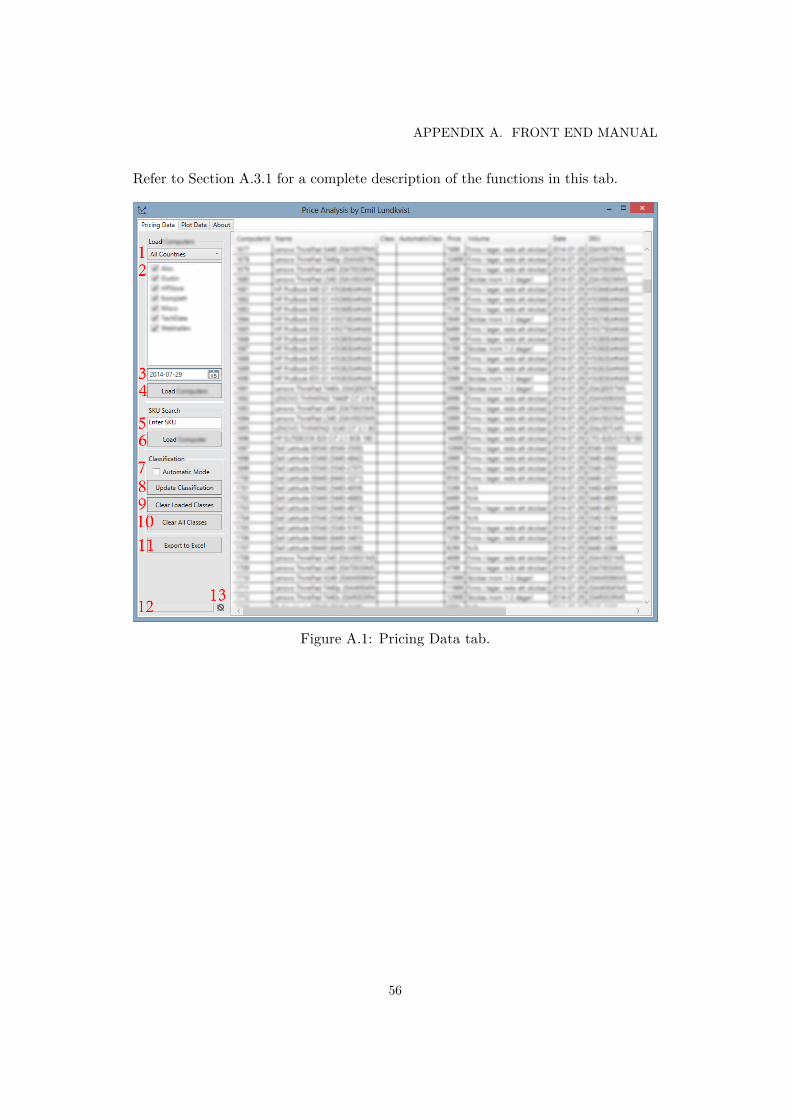
APPENDIX A. FRONT END MANUAL
Refer to Section A.3.1 for a complete description of the functions in this tab.
Figure A.1: Pricing Data tab.
56

A.2. INTERFACE
Number Name Description1 Country Combo Box. A combo box for selecting which countries
to load data from.2 Vendor Check Boxes. Check boxes for selecting which vendors
to load data from.3 Date Picker. A date picker for selecting which date to
load data from.4 Load Products Button. If this button is pressed, the products
from the selected countries and vendorsare loaded at the selected date.
5 SKU Text Box. A text box for entering a SKU for a prod-uct to load.
6 Load Product Button. If this button is pressed, the product withthe SKU in the SKU Text Box is loadedfor all countries and vendors where it ex-ists.
7 Automatic ModeCheck Box.
If this check box is selected when the Up-date Classification Button is pressed, theprogram will fill in the AutomaticClasscolumn in the results view with classes.
8 Update ClassificationButton.
If this button is pressed, the classes man-ually set in the Class column in the resultsview will be saved to the database.
9 Clear Loaded ClassesButton.
If this button is pressed, all the productsloaded in the results view will have theirclasses cleared.
10 Clear All Classes But-ton.
If this button is pressed, all product in thedatabase will have their classes cleared.
11 Export to Excel But-ton.
If this button is pressed, all data in the re-sults view is exported to an Excel spread-sheet.
12 Progress Bar. This progress bar shows when the pro-gram is busy and gives an indication ofhow long the action will take.
13 Cancel Action Button. When this button is red it is possible tocancel the current action by pressing it. Ifit is grey, there is no action to cancel.
Table A.1: Description of control elements in the Pricing Data tab.
57

APPENDIX A. FRONT END MANUAL
Column DescriptionAttribute 1. Description 1.Attribute 2. Description 2.Attribute 3. Description 3.Attribute 4. Description 4.Attribute 5. Description 5.Attribute 6. Description 6.Attribute 7. Description 7.Attribute 8. Description 8.Attribute 9. Description 9.Attribute 10. Description 10.
Table A.2: Column information in the results view.
58

A.2. INTERFACE
A.2.2 Plot Data
Figure A.2 shows the Plot Data tab. To the left in the tab there are several controlelements and to the right in the tab there is a graph view. The control elementsare described in Table A.3 and information about how to use the graph view inSection A.2.2.
The following main actions can be performed in this tab:
• Plot product pricing information for SKUs or classes.
• Plot product pricing forecasts for classes.
Refer to Section A.3.2 for a complete description of the functions in this tab.
Figure A.2: Plot Data tab.
59
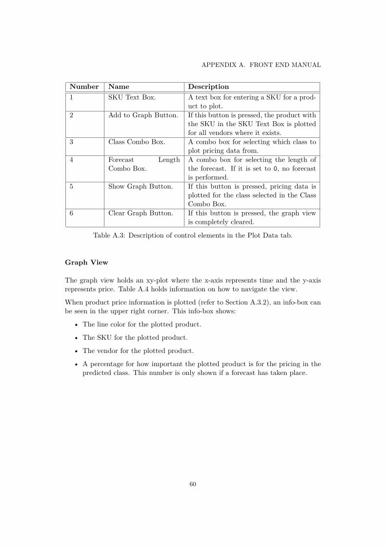
APPENDIX A. FRONT END MANUAL
Number Name Description1 SKU Text Box. A text box for entering a SKU for a prod-
uct to plot.2 Add to Graph Button. If this button is pressed, the product with
the SKU in the SKU Text Box is plottedfor all vendors where it exists.
3 Class Combo Box. A combo box for selecting which class toplot pricing data from.
4 Forecast LengthCombo Box.
A combo box for selecting the length ofthe forecast. If it is set to 0, no forecastis performed.
5 Show Graph Button. If this button is pressed, pricing data isplotted for the class selected in the ClassCombo Box.
6 Clear Graph Button. If this button is pressed, the graph viewis completely cleared.
Table A.3: Description of control elements in the Plot Data tab.
Graph View
The graph view holds an xy-plot where the x-axis represents time and the y-axisrepresents price. Table A.4 holds information on how to navigate the view.
When product price information is plotted (refer to Section A.3.2), an info-box canbe seen in the upper right corner. This info-box shows:
• The line color for the plotted product.
• The SKU for the plotted product.
• The vendor for the plotted product.
• A percentage for how important the plotted product is for the pricing in thepredicted class. This number is only shown if a forecast has taken place.
60

A.3. FUNCTIONS
Navigation Mouse KeyboardZoom Scroll up to zoom in,
scroll down to zoomout.
Press + to zoom in, − to zoom out.
Select Area Hold down scroll wheel,select an area and re-lease.
Not available.
Translate Hold right mousebutton and move themouse.
Use the arrow keys.
Show Info Hold left mouse buttonon a price line to get de-tailed info.
Not available.
Table A.4: Navigation in the graph view.
A.3 Functions
A.3.1 Pricing Data
Load All Products From Selected Vendors
1. Select “All Countries” from the Country Combo Box to load products fromall countries, or select a specific country.
2. Select which vendors to load products among the Vendor Check Boxes.
3. Select which date to load pricing information from with the Date Packer.
4. Press the Load Products Button to display the products in the display view.
Load All Products With a Selected SKU
1. Enter the SKU for a specific product in the SKU Text Box.
2. Press the Load Product Button to display the latest prices for the product ateach vendor where it exists in the database.
Classify Products
1. Load products into the data view by following the instructions in the previoussections.
61

APPENDIX A. FRONT END MANUAL
2. Fill the Class column in the data view for the products that should be classi-fied.
3. Press the Update Classification Button to save the classes to the database.
Automatic Mode If the Automatic Mode Checkbox is checked when pressingthe Update Classification Button, the program will automatically fill the Auto-maticClass column in the data view with class suggestions. These suggestions arecalculated from the available information in the Class column. This means that alarger amount of products with a class will make the suggested classes more help-ful.
Export Data to Excel
To export data to Excel, simply press the Export to Excel Button. It will open anew Excel spreadsheet with the information displayed in the data view. If there isa large amount of data in the data view, the action can take a couple of seconds tocomplete.
A.3.2 Plot Data
Plot Price for Products With a Selected SKU
1. Enter the SKU for a specific product in the SKU Text Box.
2. Press the Add to Graph Button to plot prices for the product at each vendorwhere it exists in the database.
Plot Price for Products Within a Selected Class
1. Select a class in the Class Combo Box.
2. Press the Show Graph Button to plot prices for the products in the selectedclass.
Show Price Forecast for Products Within a Selected Class
1. Select a class in the Class Combo Box.
2. Select a forecast length larger than zero in the Forecast Length Combo Box.
3. Press the Show Graph Button to plot prices and forecasts for the products inthe selected class.
62

A.3. FUNCTIONS
Clear the Graph
To clear the graph, press the Clear Graph Button.
63


Bibliography
[1] Accord.NET. C4.5. 2014. url: https://github.com/accord-net/framework/blob/development/Sources/Accord.MachineLearning/DecisionTrees/Learning/C45Learning.cs.
[2] Accord.NET. Framework. 2014. url: http://accord-framework.net/.[3] H. Akaike. “A new look at the statistical model identification”. In: IEEE
Transactions on Automatic Control 19.6 (Dec. 6, 1974), pp. 716–723.[4] E. Alpaydin. Introduction to Machine Learning. 2nd ed. The MIT Press, 2010.[5] Attivo Classification Engine. 2014. url: http://www.attivio.com/how-we-
do-it/key-differentiators/classification-engine.[6] M. J. Azur et al. “Multiple imputation by chained equations: what is it and
how does it work?” In: International journal of methods in psychiatric research20.1 (2011), pp. 40–49.
[7] L. Brailovskiy and Dr. M. Herman. “Prediction of Financial Time Series UsingHidden Markov Models”. In: Stanford University, 2014.
[8] P. J. Brockwell and R. A. Davis. Introduction to time series and forecasting.Springer New York, 1996.
[9] P. J. Brockwell and R. A. Davis. Time Series: Theory and Methods. SpringerNew York, 1986.
[10] L. Cao and F. E. H. Tay. “Financial Forecasting Using Support Vector Ma-chines”. In: Neural Comput and Applic 10 (2001), pp. 184–192.
[11] E. F. Codd. “A Relational Model of Data for Large Shared Data Banks”. In:Commun. ACM 13.6 (June 1970), pp. 377–387.
[12] J. Grandell. Formulas and survey Time series analysis. 2014. url: http ://www.math.kth.se/matstat/gru/sf2943/tsform.pdf.
[13] C. W. J. Granger. “Testing for causality : A personal viewpoint”. In: Journalof Economic Dynamics and Control 2.1 (May 1980), pp. 329–352.
[14] T. Hastie, R. Tibshirani, and J. Friedman. The elements of statistical learning:data mining, inference and prediction. 2nd ed. Springer, 2009.
[15] Ipredict. 2014. url: http://www.ipredict.it/.[16] S. B. Kotsiantis. “Supervised Machine Learning: A Review of Classification
Techniques”. In: Proceedings of the 2007 Conference on Emerging Artificial In-telligence Applications in Computer Engineering: Real Word AI Systems withApplications in eHealth, HCI, Information Retrieval and Pervasive Technolo-
65

BIBLIOGRAPHY
gies. Amsterdam, The Netherlands, The Netherlands: IOS Press, 2007, pp. 3–24.
[17] L. Ljung. System identification - Theory for the User. Prentice-Hall, 1999.[18] H. Lütkepohl. New Introduction to Multiple Time Series Analysis. Springer
Publishing Company, 2007.[19] H. Madsen. Time Series Analysis. Chapman & Hall/CRC Texts in Statistical
Science. Taylor & Francis, 2007.[20] MathWorks. Supervised Learning (Machine Learning) Workflow and Algo-
rithms. 2014. url: http://www.mathworks.co.uk/help/stats/supervised-learning-machine-learning-workflow-and-algorithms.html.
[21] Microsoft. Blend. 2014. url: http://msdn.microsoft.com/en-us/library/jj129478.aspx.
[22] Microsoft. Serialization. 2014. url: http://msdn.microsoft.com/en-us/library/ms233843.aspx.
[23] Microsoft. SQL Server. 2014. url: http://msdn.microsoft.com/en-us/library/bb545450.aspx.
[24] Microsoft. TFS Server. 2014. url: http://msdn.microsoft.com/en-us/library/ms181238(v=vs.90).aspx.
[25] Microsoft. Visual C#. 2014. url: http://msdn.microsoft.com/en- us/vstudio/hh341490.aspx.
[26] Microsoft. Visual Studio. 2014. url: http://msdn.microsoft.com/en-us/vstudio/cc136611.aspx.
[27] Microsoft. Windows Presentation Foundation. 2014. url: http : / / msdn .microsoft.com/en-us/library/ms754130(v=vs.110).aspx.
[28] J. Nielsen. Usability Engineering. San Francisco, CA, USA: Morgan KaufmannPublishers, 1993.
[29] CERN press office. CERN experiments observe particle consistent with long-sought Higgs boson. 2012. url: http : / / press . web . cern . ch / press -releases/2012/07/cern-experiments-observe-particle-consistent-long-sought-higgs-boson.
[30] Oxyplot. 2014. url: http://www.oxyplot.org/.[31] B. Pfaff. “VAR, SVAR and SVEC Models: Implementation Within R Package
vars”. In: Journal of Statistical Software 27.4 (2008).[32] J. R. Quinlan. C4.5: Programs for Machine Learning. San Francisco, CA,
USA: Morgan Kaufmann Publishers, 1993.[33] J. R. Quinlan. “Induction of Decision Trees”. In: MACH. LEARN 1 (1986),
pp. 81–106.[34] R Core Team. R: A Language and Environment for Statistical Computing.
R Foundation for Statistical Computing. Vienna, Austria, 2014. url: http://www.R-project.org/.
[35] R.NET. 2014. url: https://rdotnet.codeplex.com/.[36] Salford Systems Cart. 2014. url: http : / / www . salford - systems . com /
products/cart.
66

BIBLIOGRAPHY
[37] T. D. Schneider. Information Theory Primer. 2013. url: http://schneider.ncifcrf.gov/paper/primer/primer.pdf.
[38] B. E. Sørensen.Granger Causality. 2005. url: http://www.uh.edu/~bsorense/gra_caus.pdf.
[39] L. Stanca. Multivariate time series models. url: http://dipeco.economia.unimib.it/Persone/Stanca/defap/DEFAPtopicsbeamerVAR_2011_nop.pdf.
[40] Strategico. 2014. url: https://code.google.com/p/strategico/.[41] Zaitun Time Series. 2014. url: http://www.zaitunsoftware.com/.[42] G. Zhang, B. E. Patuwo, and M. Y. Hu. “Forecasting with artificial neural
networks: The state of the art”. In: International Journal of Forecasting 14(1998), pp. 35–62.
67