Decision Trees & Extensions

©GuillaumeCoqueret

supervisedlearningfactorinvesting

Decision Trees & Extensions

©GuillaumeCoqueret


Why decision trees

Several related reasons

I they are known to perform very well on structured/rectangulardata: typically the type of financial data (if we exclude alt-data)

I they (i.e., their extensions) are probably the most popularsolutions among winning solutions in Kaggle competitions

I they are often easy to understand and to interpret (at leastthrough variable importance)

2 / 27

©GuillaumeCoqueret


Agenda

1 Principle & Examples

2 Extensions

3 Variable importance

4 Wrap-up

3 / 27

©GuillaumeCoqueret


Introduction

Difference with linear approaches

Linear approach:

yi = α + β(1)x (1)i + · · ·+ β(K )x (K )

i + εi

There are much more complicated functions yi = f (xi ) + εi !Trees are models that form clusters based on x such that theclusters are homogeneous in y .In portfolio management, y is related to performance, say, return.Hence depending on x , some clusters will have low average y (e.g.,return) and others high average y . Those are the ones we will wantto invest in!

Usual non-financial example: Obama-Clinton votes from NY Times

4 / 27

https://archive.nytimes.com/www.nytimes.com/imagepages/2008/04/16/us/20080416_OBAMA_GRAPHIC.html

©GuillaumeCoqueret


A basic example

y is the colour of the star (to be predicted), x(1) is the size of the star,x(2) is the shape (complexity) of the star.

complicatedstars

simplestars

smallstars

smallstars

largestars

largestars

5 / 27

©GuillaumeCoqueret


DiamondsSplits, splits, it’a all about splits!What are the drivers of their prices? Cut, colour, clarity... size?

carat < 1

carat < 0.63 carat < 1.5

clarity = I1,SI2,SI1,VS2 carat < 1.9

3933100%

163365%

105246%

305919%

814235%

614024%

537118%

85356%

12e+312%

11e+38%

15e+34%

yes no

The size, of course, but not only!→ in rpart, from the condition under the node, it’s always: TRUE tothe left and FALSE to the right.

6 / 27

©GuillaumeCoqueret


Process (1/3)A large majority of trees work with binary splits (so will we).

A simplified case: how to choose splitting points?Imagine we work with only one explanatory variable x . In the case ofdiamonds, let’s assume we only consider the size (weight in carats). What’sthe best possible (initial) split?Since we seek homogeneous clusters, total quadratic variation/dispersionis a good start:

V (c) =∑

i:carat>c

(pi − pcarat>c)2

︸︷︷︸large diamond cluster (>c)

+∑

i:carat<c

(pi − pcarat<c)2

︸︷︷︸small diamond cluster (<c)

pcarat>c is the average price of all diamonds with weight larger than c.

This split yields a decomposition that is smaller than the original totalvariation (scaled variance): TV =

∑i (pi − p)2. The gain is

G(c) = TV − V (c)

7 / 27

©GuillaumeCoqueret


Process (2/3)

4e+11

5e+11

6e+11

7e+11

8e+11

1 2 3 4threshold

total_var

Minimum point at 1 carat. No other feature can achieve this lowlevel of total dispersion.

8 / 27

©GuillaumeCoqueret


Process (3/3)

The full splitting process can be described as:

For each node / cluster:

1. Find the best splitting point for each variable.2. Determine which variable achieves the highest gain (reduction

in loss or objective)3. Split according to this variable→ two new clusters!

This is performed until some condition is met (improvement of gainbecomes too small or sufficient depth is reached).

9 / 27

©GuillaumeCoqueret


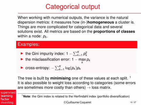
Categorical outputWhen working with numerical outputs, the variance is the naturaldispersion metrics: it measures how (in-)homogeneous a cluster is.Things are more complicated for categorical data and severalsolutions exist. All metrics are based on the proportions of classeswithin a node: pk .

Examples:

I the Gini impurity index: 1−∑K

k=1 p2k

I the misclassification error: 1−maxk

pk

I cross-entropy: −∑K

k=1 log(pk )pk

The tree is built by minimising one of these values at each split. 1

It is also possible to weight loss according to categories (some errorsare sometimes more costly than others)→ loss matrix.

1Note: the Gini index is related to the Herfindahl index (portfolio diversification)

10 / 27

©GuillaumeCoqueret


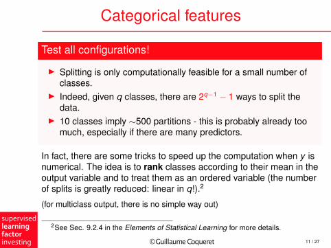
Categorical features

Test all configurations!

I Splitting is only computationally feasible for a small number ofclasses.

I Indeed, given q classes, there are 2q−1 − 1 ways to split thedata.

I 10 classes imply ∼500 partitions - this is probably already toomuch, especially if there are many predictors.

In fact, there are some tricks to speed up the computation when y isnumerical. The idea is to rank classes according to their mean in theoutput variable and to treat them as an ordered variable (the numberof splits is greatly reduced: linear in q!).2

(for multiclass output, there is no simple way out)

2See Sec. 9.2.4 in the Elements of Statistical Learning for more details.

11 / 27

©GuillaumeCoqueret


Financial dataOn rescaled features

Mkt_Cap >= 0.52

Prof_Marg < 0.35

D2E >= 0.85 P2B >= 0.98

D2E >= 0.12

P2B >= 0.12 Vol_1M < 0.82

0.0065100%

0.00250%

-0.0088%

-0.0661%

-0.00258%

0.004142%

-0.0271%

0.004641%

0.01150%

0.009848%

0.008143%

0.0226%

0.0432%

0.0111%

0.0751%

yes no

12 / 27

©GuillaumeCoqueret


Agenda


2 Extensions


4 Wrap-up

13 / 27

©GuillaumeCoqueret


Random forests (1/2)I Given one splitting rule and one dataset, there is only one

optimal tree.I RF pick random combinations of features to build aggregations

of trees. This technique is called ‘bagging’.I Each output value is the average of the outputs obtained over all

trees.

(0.1-0.05+0.25)/3 = 0.1

Tree 1 Tree 2 Tree 3

+0.1 -0.05 +0.25

(or majority voting if categorical output)

14 / 27

©GuillaumeCoqueret


Random forests (2/2)

Options when building the forests:

I fix the depth / complexity of the tree (just as for simple trees);I select the number of features to retain for each individual

learner (tree);I determine the sample size required to train the learners.

Random forests are more complex and richer than simple trees.One cool feature: RFs don’t have a huge tendency to overfit. Thus,most of the time, their performance is higher.

15 / 27

©GuillaumeCoqueret


Boosted trees: principle (1/6)

IdeaLike RFs, boosted trees aggregate trees. The model can be writtenas:

yi = mJ(xi ) =J∑

j=1

Tj (xi ),

where i is the index of the occurrence (e.g., stock-date pair) and J isthe number of trees. We thus has the following simple relationshipwhen we add trees to the model:

mJ(xi ) = mJ−1(xi )︸︷︷︸old trees

+ TJ(xi )︸︷︷︸new tree

When the previous model is built, how do we choose the new tree?→ the model is constructed iteratively.

16 / 27

©GuillaumeCoqueret


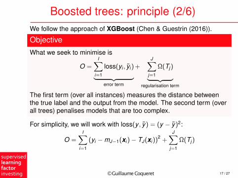
Boosted trees: principle (2/6)We follow the approach of XGBoost (Chen & Guestrin (2016)).

Objective

What we seek to minimise is

O =I∑

i=1

loss(yi , yi )︸︷︷︸error term

+J∑

j=1

Ω(Tj )︸︷︷︸regularisation term

The first term (over all instances) measures the distance betweenthe true label and the output from the model. The second term (overall trees) penalises models that are too complex.

For simplicity, we will work with loss(y , y) = (y − y)2:

O =I∑

i=1

(yi −mJ−1(xi )− TJ(xi ))2 +J∑

j=1

Ω(Tj )

17 / 27

©GuillaumeCoqueret



We have built tree TJ−1 (and hence model mJ−1): how to choose tree TJ?Decompose the objective:

O =I∑

i=1

(yi −mJ−1(xi )− TJ (xi ))2 +J∑

j=1

Ω(Tj )

=I∑

i=1

y2

i + mJ−1(xi )2 + TJ (xi )

2

+J−1∑j=1

Ω(Tj ) + Ω(TJ )

− 2I∑

i=1

yimJ−1(xi ) + yiTJ (xi )−mJ−1(xi )TJ (xi )) cross terms

=I∑

i=1

−2yiTJ (xi ) + 2mJ−1(xi )TJ (xi )) + TJ (xi )

2

+ Ω(TJ ) + c

The red terms are known at step J!→ things are simple with quadratic loss. For more complicated lossfunctions, Taylor expansions are used.

18 / 27

©GuillaumeCoqueret



We need to take care of the penalisation now. For a given tree T , wespecify tree T (x) = wq(x), where w is the output value of some leaf and q(·)is the function that maps an input to its final leaf. We write l = 1, . . . , L for theindices of the leafs of the tree. In XGBoost, complexity is defined as:

Ω(T ) = γL +λ

2

L∑l=1

w2l ,

whereI the first term penalises the total number of leavesI the second term penalises the magnitude of output values (this helps

reduce variance).

Below, we omit the index (J) of the tree of interest (i.e., the last one).Moreover, we write Il for the set of the indices of the instances belonging toleaf l .

19 / 27

©GuillaumeCoqueret


Boosted trees: principle (4b/6)

Illustration of q and w :

carat < 1

carat < 0.63 carat < 1.5

clarity = I1,SI2,SI1,VS2 carat < 1.9

3933100%

163365%

1052w

3059w

814235%

614024%

5371w

8535w

12e+312%

11e+3w

15e+3w

yes no

1 2 3 4 5 6

q(.)

q defines the pathto the leaf

20 / 27

©GuillaumeCoqueret


Boosted trees: principle (5/6)We aggregate both sections of the objective:

O = 2I∑

i=1

yiTJ (xi )−mJ−1(xi )TJ (xi )) +

TJ (xi )2

2

+ γL +

λ

2

L∑l=1

w2l

= 2I∑

i=1

yiwq(xi ) −mJ−1(xi )wq(xi )) +

w2q(xi )

2

+ γL +

λ

2

L∑l=1

w2l

= 2L∑

l=1

wl

∑i∈Il

(yi −mJ−1(xi )) +w2

l

2

∑i∈Il

(1 +

λ

2

)+ γL

→ w∗l = −∑

i∈Il(yi −mJ−1(xi ))(

1 + λ2

)#i ∈ Il

,

OL(q) = −12

L∑l=1

(∑i∈Il

(yi −mJ−1(xi )))2

(1 + λ

2

)#i ∈ Il

+ γL

which gives the optimal weights (or leaf scores) and objective value.3

3f (x) = ax + b2 x2: min at x∗ = −a/b, min value = −a2/(2b).

21 / 27

©GuillaumeCoqueret


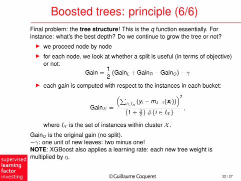
Boosted trees: principle (6/6)Final problem: the tree structure! This is the q function essentially. Forinstance: what’s the best depth? Do we continue to grow the tree or not?I we proceed node by nodeI for each node, we look at whether a split is useful (in terms of objective)

or not:Gain =

12

(GainL + GainR −GainO)− γ

I each gain is computed with respect to the instances in each bucket:

GainX =

(∑i∈IX

(yi −mJ−1(xi )))2

(1 + λ

2

)#i ∈ IX

,

where IX is the set of instances within cluster X .

GainO is the original gain (no split).−γ: one unit of new leaves: two minus one!NOTE: XGBoost also applies a learning rate: each new tree weight ismultiplied by η.

22 / 27

©GuillaumeCoqueret


Interpretability!

Definition = gain allocation!

I Each time a split is performed according to one variable/feature,the objective function is reduced

I This gain is entirely attributed to the variableI If we sum the gains obtained by all variables over all trees and

normalise them in the cross-section of features, we get therelative importance of each feature!

Vf ∝N∑

n=1

Gn(f ),

where f is the index of the feature and Gn(f ) the gain associated tofeature f at node n (positive if the split is performed according to fand zero otherwise).

24 / 27

©GuillaumeCoqueret


Key takeaways

Trees are powerful

I they organise the data into homogeneous clusters in a highlynonlinear fashion

I extensions help improve the predictive performance byaggregating several trees

I variable importance is a first step towards interpretability(global in this case)

26 / 27

Decision Trees & Extensions

Documents

Transcript of Decision Trees & Extensions