Decision Procedures for Presburger Arithmetic

Presented by Constantinos Bartzis

Presburger formulas

numeral ::= 0 | 1 | 2…

var ::= x | y | z …

relop ::= < | ≤ | = | | >

term ::= numeral | var | term + term | -term | numeral term

formula ::= term relop term | formula formula | formula formula | formula | var. formula | var. formula

numeral term isn't really multiplication; it's short-hand for term + term + … + term

Decision Procedures

Will discuss algorithms for determining truth of formulas of Presburger arithmetic: Fourier-Motzkin variable elimination (FMVE) Omega Test Cooper's algorithm Automata based

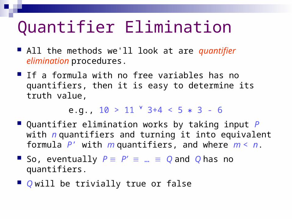
Quantifier Elimination All the methods we'll look at are quantifier elimination

procedures.

If a formula with no free variables has no quantifiers, then it is easy to determine its truth value,

e.g., 10 > 11 3+4 < 5 3 - 6

Quantifier elimination works by taking input P with n quantifiers and turning it into equivalent formula P’ with m quantifiers, and where m < n.

So, eventually P P’ … Q and Q has no quantifiers.

Q will be trivially true or false

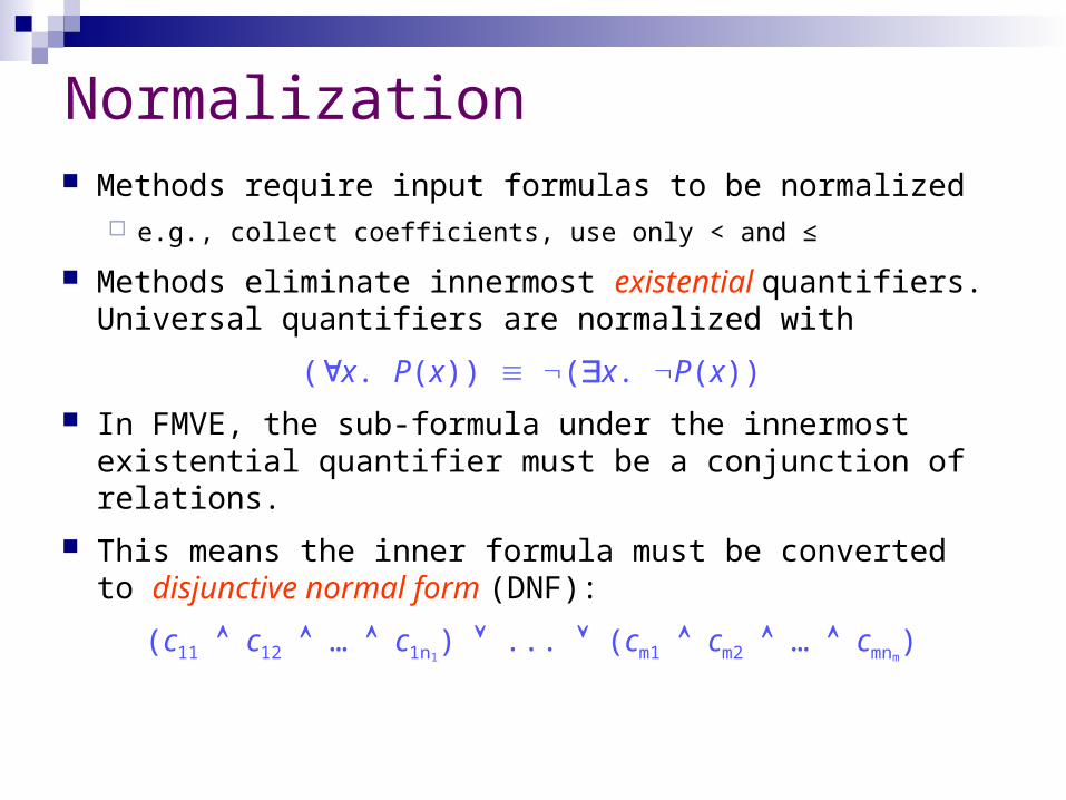
Normalization Methods require input formulas to be normalized

e.g., collect coefficients, use only < and ≤

Methods eliminate innermost existential quantifiers. Universal quantifiers are normalized with

(x. P(x)) (x. P(x))

In FMVE, the sub-formula under the innermost existential quantifier must be a conjunction of relations.

This means the inner formula must be converted to disjunctive normal form (DNF):

(c11 c12 … c1n1) ... (cm1 cm2 … cmnm

)

Normalization (cont.) The formula under is in DNF. Next, the must be

moved inwards First over disjuncts, using

(x. P Q) (x. P) (x. Q) Must then ensure every conjunct under the quantifier

mentions the bound variable. Use

(x. P(x) Q) (x. P(x)) Q For example:

(x. 3 < x x +2y ≤ 6 y < 0) (x. 3 < x x +2y ≤ 6) y < 0

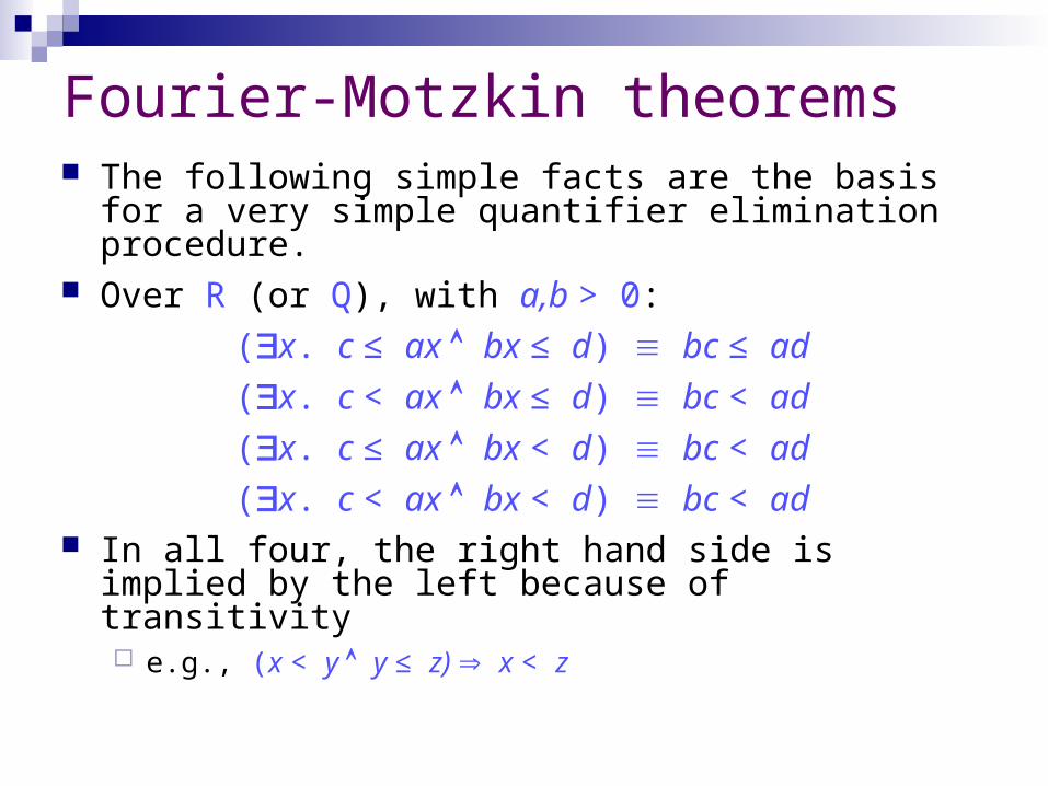
Fourier-Motzkin theorems The following simple facts are the basis for a very simple

quantifier elimination procedure. Over R (or Q), with a,b > 0:

(x. c ≤ ax bx ≤ d) bc ≤ ad

(x. c < ax bx ≤ d) bc < ad

(x. c ≤ ax bx < d) bc < ad

(x. c < ax bx < d) bc < ad In all four, the right hand side is implied by the left

because of transitivity e.g., (x < y y ≤ z) x < z

Fourier-Motzkin theorems (cont.) For the other direction:

(bc < ad) (x. c < ax bx ≤ d)

take x to be d/b : c < a( d/b ), and b( d/b ) ≤ d. For (bc < ad) (x. c < ax bx < d)

take x to be (bc+ad)/2ab :

c < a(bc+ad)/2ab 2bc < bc+ad bc < ad Similarly for the other bound

Extending to a full procedure So far: a quantifier elimination procedure for formulas

where the scope of each quantifier is 1 upper bound and 1 lower bound.

We need to extend the method to cover cases with multiple constraints.

No lower bound, many upper bounds:

(x: b1x < d1 b2x < d2 … bnx < dn)

True! (take min(di/bi) as a witness for x)

No upper bound, many lower bounds: obviously analogous.

Combining many constraints Example:

(x. c ≤ ax b1x ≤ d1 b2x ≤ d2) b1c ≤ ad1 b2c ≤ ad2

From left to right, the result just depends on transitivity.

From right to left, take x to be min(d1/b1, d2/b2).

In general, with many constraints, combine all possible lower-upper bound pairs.

Proof that this is possible is by induction on the number of constraints.

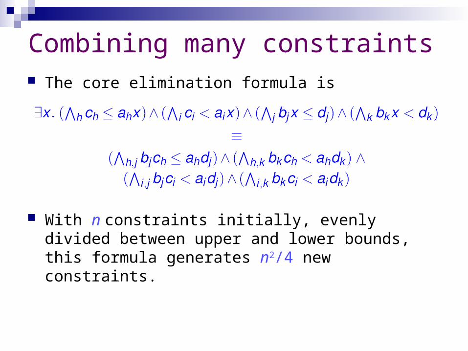
Combining many constraints The core elimination formula is

With n constraints initially, evenly divided between upper and lower bounds, this formula generates n2/4 new constraints.

FMVE example

x. 20+x ≤ 0 y. 3y +x ≤ 10 20 ≤ y - x(re-arrange) x. 20+x ≤ 0 y. 20+x ≤ y 3y ≤ 10 - x(eliminate y) x. 20+x ≤ 0 60+3x ≤ 10 - x(re-arrange) x. 20+x ≤ 0 4x +50 ≤ 0(normalize universal) x. 20+x ≤ 0 0 < 4x +50(re-arrange) x. -50 < 4x x ≤ -20(eliminate x) (-50 < -80) T

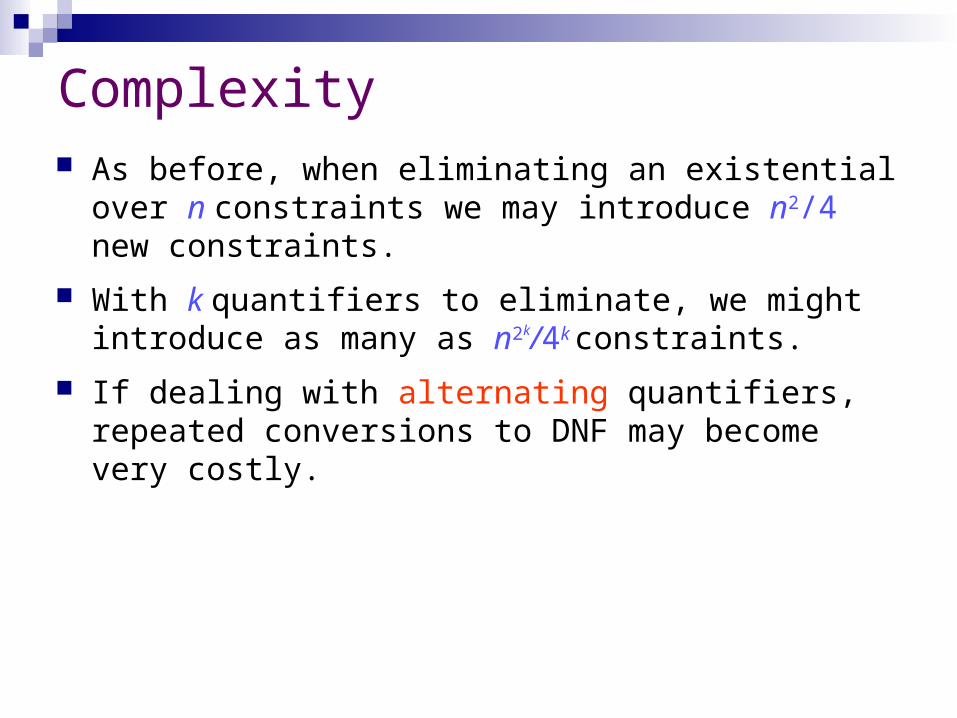
Complexity As before, when eliminating an existential over n

constraints we may introduce n2/4 new constraints.

With k quantifiers to eliminate, we might introduce as many as n2k/4k constraints.

If dealing with alternating quantifiers, repeated conversions to DNF may become very costly.

Integers

Expressiveness over Integers Can do divisibility by specific numerals:

2|e x. 2x = e

for example:

x. 0 < x < 30 (2|x 3|x 5|x) Can do integer division and modulus, as long as divisor

is constant. Use one of the following results (similar for division)

P(x mod d) q,r. (x = qd +r ) (0 ≤ r < d d < r ≤ 0) P(r )

P(x mod d) q,r. (x = qd +r ) (0 ≤ r < d d < r ≤ 0) P(r )

Any formula involving modulus or integer division by a constant can be translated to one without.

Expressivity over Integers Any procedure for Z trivially can be extended to

one for N (or any mixture of N and Z) too: Add extra constraints stating that variables are 0

Relations < and ≤ can be converted into one another:

x ≤ y x < y +1

x < y x +1 ≤ y

Decision procedures normalize to one of these relations.

Fourier-Motzkin for Integers? Central theorem is false. E.g.,

(xZ. 3 ≤ 2x 2x ≤ 3) 6 ≤ 6

But one direction still works (thanks to transitivity):

( x. c ≤ ax bx ≤ d) bc ≤ ad

We can compute consequences of existentially quantified formulas

/

Fourier-Motzkin for Integers? We know (x. c ≤ ax bx ≤ d) bc ≤ ad Thus an incomplete procedure for universal formulas

over Z: Compute negation: (x. P(x)) (x. P(x)) Compute consequences:

if (x. P(x)) then (x. P(x)) and (x. P(x)) T Repeat for all quantified variables. This is Phase 1 of the Omega Test

Omega Phase 1 - Example

x,yZ. 0 < x y < x y +1 < 2x

(normalize)

x,y. 1 ≤ x y +1 ≤ x 2x ≤ y +1

x,y. 1 ≤ x y +1 ≤ x 2x ≤ y +1

(eliminate y)

x. 1 ≤ x 2x ≤ x

(normalize)

x. 1 ≤ x x ≤ 0

(eliminate x)

1 ≤ 0

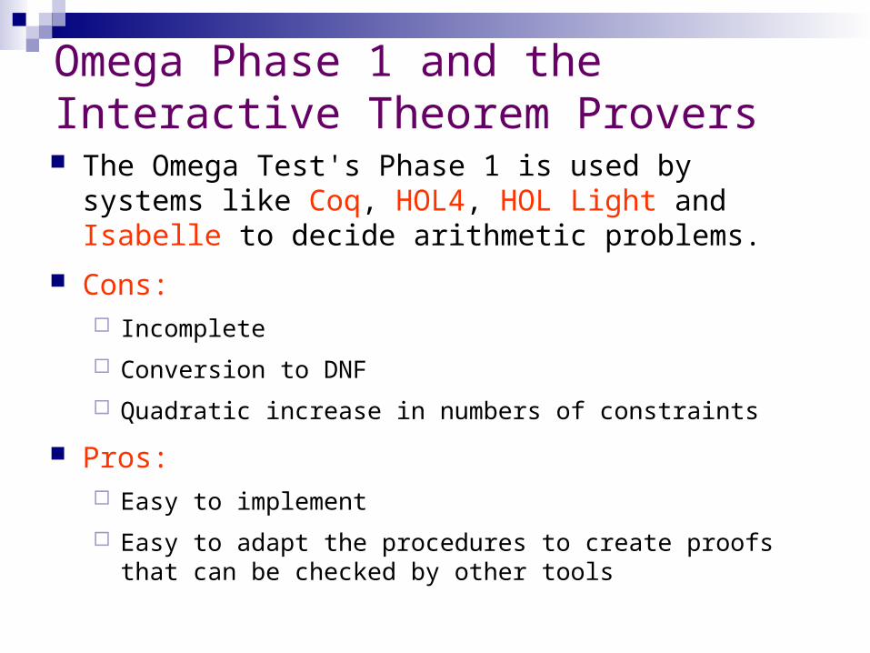
Omega Phase 1 and the Interactive Theorem Provers The Omega Test's Phase 1 is used by systems like Coq,

HOL4, HOL Light and Isabelle to decide arithmetic problems.

Cons: Incomplete

Conversion to DNF

Quadratic increase in numbers of constraints

Pros: Easy to implement

Easy to adapt the procedures to create proofs that can be checked by other tools

Some Shadows

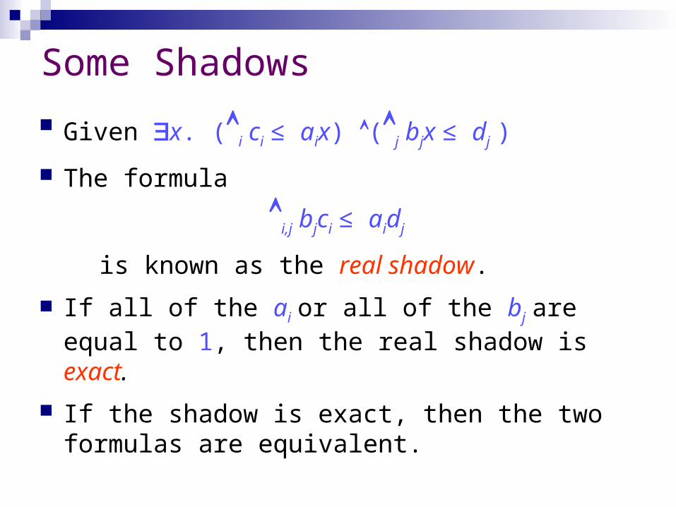
Given x. (i ci ≤ aix) (j bjx ≤ dj )

The formula

i,j bjci ≤ aidj

is known as the real shadow.

If all of the ai or all of the bj are equal to 1, then the real shadow is exact.

If the shadow is exact, then the two formulas are equivalent.

Exact Shadows When a = 1 or b = 1, the core theorem (x. c ≤ ax bx ≤ d) bc ≤ ad is valid because

transitivity still holds

take x = d if b = 1 or x = c if a = 1

Omega Test's inventor, Bill Pugh, claims many problems in his domain (compiler optimization) have exact shadows.

Experience suggests the same is true in other domains too, such as hardware model checking.

When shadows are exact, we can pretend the problem is over R rather than Z and proceed as before.

Dark Shadows The formula i,j (ai-1)(bj-1) ≤ aidj - bjci

is known as the dark shadow.

If all ai or all bj are one, then this is the same as the real shadow (or exact).

The real shadow provides a test for unsatisfiability. The dark shadow tests for satisfiability, because

(a-1)(b-1) ≤ ad - bc (x. c ≤ ax bx ≤ d) This is the Phase 2 of the Omega Test

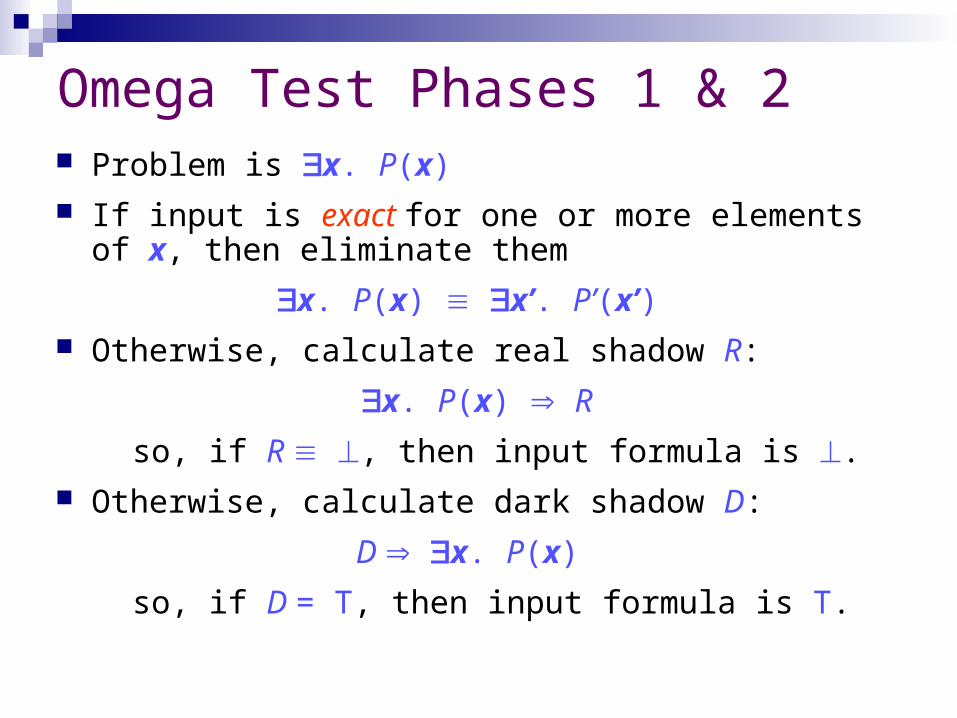
Omega Test Phases 1 & 2 Problem is x. P(x) If input is exact for one or more elements of x, then

eliminate them

x. P(x) x’. P’(x’) Otherwise, calculate real shadow R:

x. P(x) R

so, if R , then input formula is . Otherwise, calculate dark shadow D:

D x. P(x)

so, if D = T, then input formula is T.

Omega Phase 2 - Example(a-1)(b-1) ≤ ad - bc (x. c ≤ ax bx ≤ d)

x,y. 3x +2y ≤ 18 3y ≤ 4x 3x ≤ 2y +1

3y ≤ 4x 3x ≤ 2y +1 3y ≤ 4x 3x ≤ 18 - 2y

6 ≤ 8y + 4 - 9y 6 ≤ 72 - 8y - 9y

y ≤ -2 17y ≤ 66

y ≤ 3 This gives a suitable value for y, and by back-

substitution, finds

x = -1, y = -2 as a possible solution.

Splinters Purely existential formulas are often proved false by their

real shadow; or proved true by their dark shadow

But in “rare” cases, the main theorem is needed. Let m be the maximum of all the djs. Then

dark shadowsplinter

Splinters A splinter does represent a smaller problem than

the original because the extra equality allows x to be eliminated immediately.

When quantifiers alternate, and there is no exact shadow, the main theorem is used as an equivalence, and splinters can't be avoided.

Splinters must also be checked if neither real nor dark shadows decide an input formula.

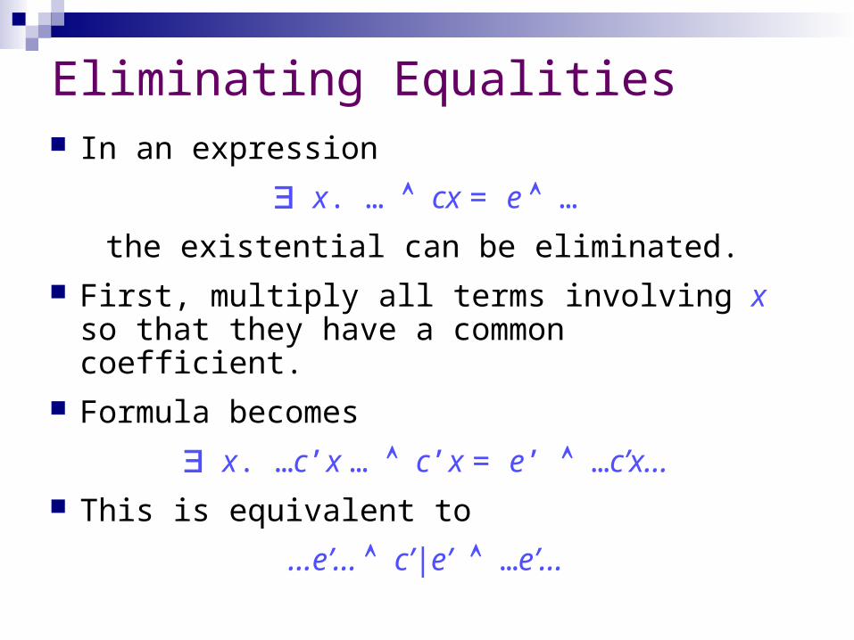
Eliminating Equalities In an expression

x. … cx = e …

the existential can be eliminated. First, multiply all terms involving x so that they

have a common coefficient. Formula becomes

x. …c’x … c’x = e’ …c’x… This is equivalent to

…e’… c’|e’ …e’…

Eliminating Divisibilitiesx. … c | dx + e …

Note: d < c (otherwise, replace d with d mod c). Introduce temporary new existential variable:

x,y. … cy = dx + e … Rearrange:

x,y. … dx = cy -e … Use equality elimination to derive

y. … d | cy -e … Because d < c, this process must terminate with

elimination of divisibility term.

Implementation - Normalization Omega Test's main disadvantage is that it requires the

matrix of the formula to be in DNF

Consider

x. (x 10 x 11 9 < x ≤ 12) x = 12

Negate, remove , <:

x. (x ≤ 9 11 ≤ x) (x ≤ 10 12 ≤ x) 10 ≤ x x ≤ 12 (x ≤ 11 13 ≤ x)

Evaluate 8 (= 23) DNF terms.

Clever preparation of input formulas can make orders of magnitude difference

Implementation - Normalization The propositional tautology

(p (q q’)) (p q p q’)

justifies the following procedure: If P is an atomic formula, then when processing P Q,

assume P is true while processing Q: If a sub-formula Q0 of Q is such that P Q0, then replace Q0 in

Q by T.

If a sub-formula Q0 of Q is such that P Q0, then replace Q0 in

Q by .

Similarly, (p (q q’)) (p q p q’) for disjunctions.

Example Over :

0 ≤ x + y + 4 (0 ≤ x + y + 6 0 ≤ 2x + 3y + 6)

is equivalent to 0 ≤ x + y + 4 Whereas

0 ≤ x + y + 4 0 ≤ -x -y -6 0 ≤ 2x + 3y + 6

is equivalent to Over :

0 ≤ x + y + 4 0 ≤ x + y + 1 0 ≤ 2x + 3y + 6

is equivalent to

0 ≤ x + y + 4 0 ≤ 2x + 3y + 6

Cooper’s Algorithm

Cooper's Algorithm Cooper's algorithm is a decision procedure for

Presburger arithmetic. A non-Fourier-Motzkin alternative It is also a quantifier elimination procedure, which

also works from the inside out, eliminating existentials.

Its advantage is that it doesn't need to normalize input formulas to DNF.

Description is of simplest possible implementation; many tweaks are possible.

Preprocessing To eliminate the quantifier in x. P(x):

1. Normalize so that only operators are <, and divisibility (c|e), and negations only occur around divisibility leaves.

2. Compute least common multiple c of all coefficients of x, and multiply all terms by appropriate numbers so that in every term the coefficient of x is c.

3. Now apply

( x. P(cx)) ( x. P(x) c|x).

Preprocessing Example

x,y Z. 0 < y x < y x +1 < 2y

(normalize)

x,y. 0 < y x < y 2y < x +2

(transform y to 2y everywhere)

x,y. 0 < 2y 2x < 2y 2y < x +2

(give y unit coefficient)

x,y. 0 < y 2x < y y < x +2 2|y

Two ways How might x. P(x) be true?

Either: there is a least x making P true; or

there is no least x: however small you go, there will be a smaller x that still makes P true

Construct two formulas corresponding to both cases.

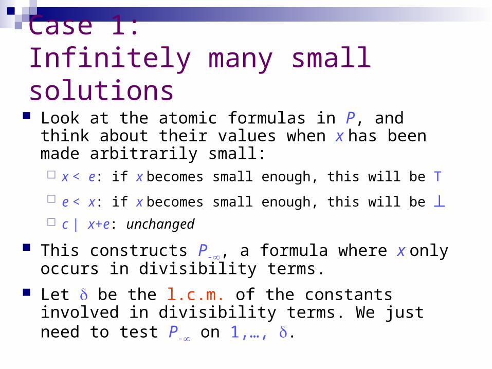
Case 1:Infinitely many small solutions

Look at the atomic formulas in P, and think about their values when x has been made arbitrarily small: x < e: if x becomes small enough, this will be T

e < x: if x becomes small enough, this will be c | x+e: unchanged

This constructs P-, a formula where x only occurs in divisibility terms.

Let be the l.c.m. of the constants involved in divisibility terms. We just need to test P- on 1,…, .

P- example

For y. 0 < y 2x < y y < x +2 2|y 0 < y will become as y gets small

2x < y also becomes as y gets small

y < x +2 will be T as y gets small

2|y doesn't change (it tests if y is even or not)

So in this case,

P- (y) ( T 2|y)

Case 2: Least solution exists The case when there is a least x satisfying P(x).

For there to be a least x satisfying P(x), it must be the case that one of the terms e < x is T, and that if x was any smaller the formula would become .

Let B = {b | b < x is a term of P(x)}

Need just consider P(b+j), where b B and 1 ≤ j ≤ .

Final elimination formula is:

Example continued For

y. 0 < y 2x < y y < x +2 2|y

least solutions, if they exist, will be at

y = 1, y = 2, y = 2x +1, or y = 2x +2

The divisibility constraint eliminates two of these.

Original formula is equivalent to:

(2x < 2 0 < x) (0 < 2x +2 x < 0)

Which is unsatisfiable.

Automata based

Symbolic Representation

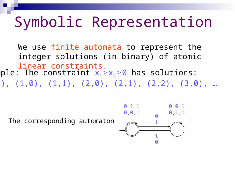
We use finite automata to represent the integer solutions (in binary) of atomic linear constraints.

0 1 10,0,1

0 0 10,1,1

01

10

Example: The constraint x1x20 has solutions:(0,0), (1,0), (1,1), (2,0), (2,1), (2,2), (3,0), …

The corresponding automaton

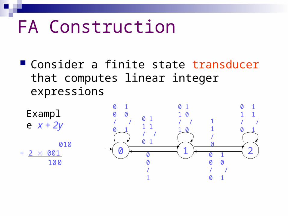
FA Construction

Consider a finite state transducer that computes linear integer expressions

0 1 2

0 10 0/ /0 1

01/ 1

0 11 1/ /0 1

0 10 0/ /0 1

11 /1

1 1 / 0

00/1

Example x + 2y

010+ 2 001

10 0

01/ 0

10 /0

Equality with 0

Remove transitions that write 1.

Make state 0 accepting

states

0 1 -1

0 10 0/ /0 1

01/ 1

0 11 1/ /0 1

0 10 0/ /0 1

11 /1

1 1 / 0

00/0

01/ 0

10 /0

| |ii

v

a

1

1

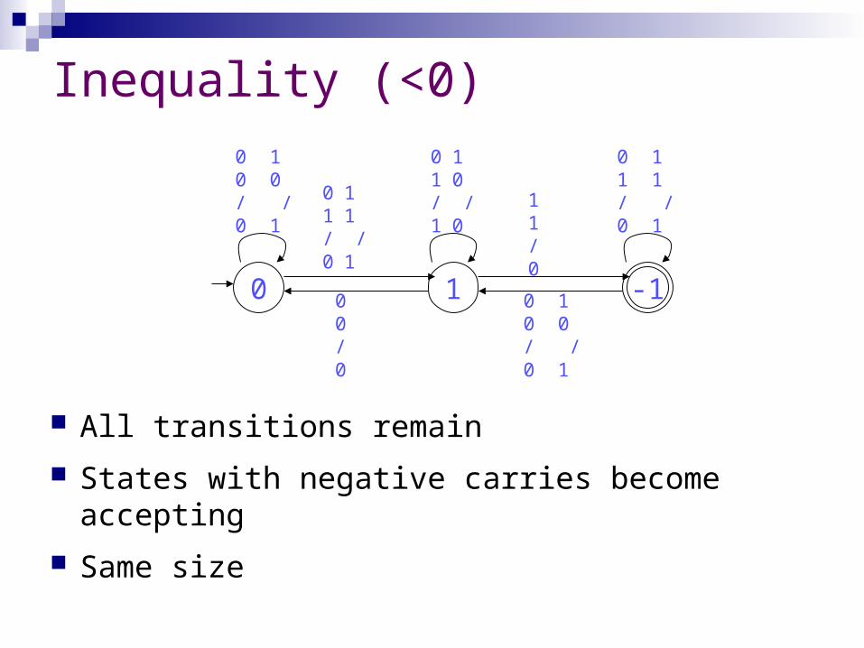
Inequality (<0)

All transitions remain

States with negative carries become accepting

Same size

0 1 -1

0 10 0/ /0 1

01/ 1

0 11 1/ /0 1

0 10 0/ /0 1

11 /1

1 1 / 0

00/0

01/ 0

10 /0

Non-zero Constant Term c

Same as before but now -c is the initial state

If there is no such state, create one (and possibly some intermediate states)

Size | | | |ii

v

a c

1

0 1 -1

0 10 0/ /0 1

01/ 1

0 11 1/ /0 1

0 10 0/ /0 1

11 /1

1 1 / 0

00/0

01/ 0

10 /0

Boolean Connectives

For compute the intersection

For compute the union

For compute the complement

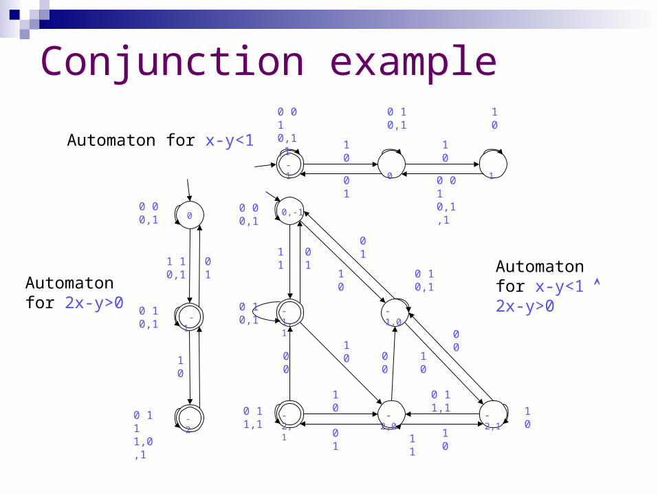
Conjunction example0 0 10,1,1

0 10,1

10

10

10

01

0 0 10,1,1

Automaton for x-y<1-1

0 1

0 00,1

0 10,1

0 1 11,0,1

1 10,1

01

10

Automatonfor 2x-y>0

0

-1

-2

11

01

10

00

0 00,1

11

10

10

01

0 10,1

0 11,1

10

00

00

0 10,1

10

01

0 11,1 1

0

Automaton for x-y<1 2x-y>0-1,-

1

0,-1

-2,-1

-1,0

-2,0

-2,1

Existential Quantifier Elimination

To eliminate x, remove the track of x

The resulting FA is in general non-deterministic

Determinization may cause exponential blowup

Rarely occurs in practice

0 0 10,1,1

0 10,1

10

10

10

01

0 0 10,1,1

x . x-y<1-1

0

1

Extensions / Improvements

Using 2’s complement representation the method can be extended to all integers by just doubling the size of the automaton.

Can also be extended to rationals, using automata on infinite words.

Quantifier elimination can be done in linear time if the existential variable appears in an equation with odd coefficient.

Currently outperforms Omega, but loses to DPLL(T) methods for quantifier-free inputs.

Questions?