DECISION MODELINGDECISION MODELING

Chapter 2

Spreadsheet Modeling

Part 1

WITH WITH MICROSOFT EXCELMICROSOFT EXCEL

Copyright 2001Prentice Hall Publishers and

Ardith E. Baker

In building spreadsheets for deterministic models, we will look at:

ways to translate the black box representation into a spreadsheet model.

recommendations for good spreadsheet model design and layout

suggestions for documenting your models

useful features of Excel for modeling and analysis

Step 1: Study the Environment and Frame the Situation

The Pies are then processed and sold to local grocery stores in order to generate a profit.

Follow the three steps of model building.

Example 1: Simon Pie

Critical Decision: Setting the wholesale pie price

Decision Variable: Price of the apple pies (this plus cost parameters will determine profits)

Two ingredients combine to make Apple Pies: Fruit and frozen dough

Step 2: Formulation

Model

Using “Black Box” diagram, specify cost parameters

The next step is to develop the logic inside the black box.

A good way to approach this is to create an Influence Diagram.

Pie PriceUnit Cost, FillingUnit Cost, Dough

Unit Pie Processing CostFixed Cost

An Influence Diagram pictures the connections between the model’s exogenous variables and a performance measure (e.g., profit).

Exogenous Variables

To create an Influence Diagram:start with a performance measure variable.

Further decompose each of the intermediate variables into more related intermediate variables.

Decompose this variable into two or more intermediate variables that combine mathematically to define the value of the performance measure.

Continue this process until an exogenous variable is defined (i.e., until you define an input decision variable or a parameter).

performance measure variable

ProfitStart here:

Decompose this variable into the intermediate variables Revenue and Total Cost

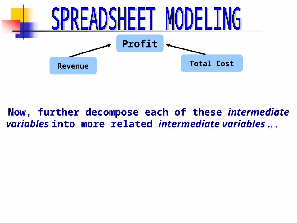
Profit

Revenue Total Cost

Now, further decompose each of these intermediate variables into more related

intermediate variables ...

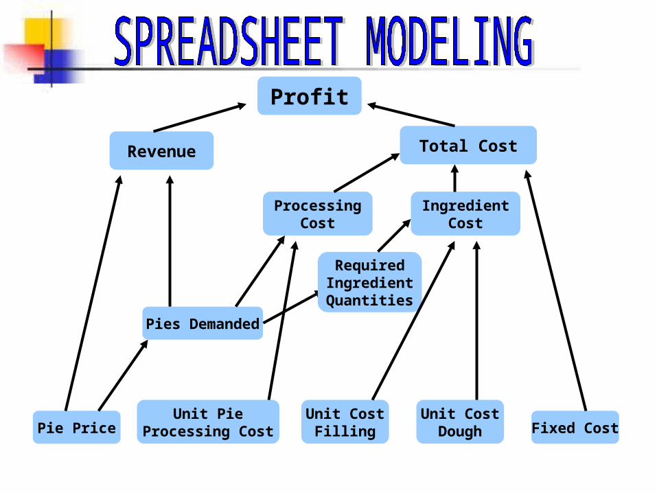
Profit

Revenue Total Cost

Pies Demanded

Pie PriceUnit Pie

Processing Cost Fixed Cost

ProcessingCost

IngredientCost

Unit CostFilling

Unit CostDough

RequiredIngredientQuantities

Step 3: Model Construction

Based on the previous Influence Diagram, create the equations relating the variables to be specified in the spreadsheet.

Profit

Revenue Total Cost

Profit = Revenue – Total Cost

Profit

Revenue

Pie Price

Pies Demanded

Revenue = Pie Price * Pies Demanded

Fixed Cost

ProcessingCost

IngredientCost

Profit

Total Cost

Total Cost = Processing Cost + Ingredients Cost + Fixed Cost

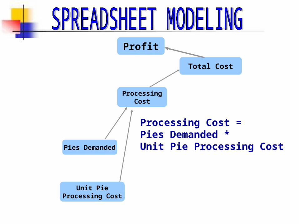
Processing Cost = Pies Demanded * Unit Pie Processing Cost

ProcessingCost

Total Cost

Pies Demanded

Unit PieProcessing Cost

Profit

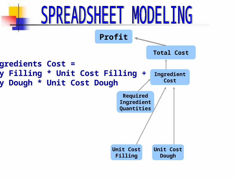
Ingredients Cost = Qty Filling * Unit Cost Filling + Qty Dough * Unit Cost Dough

IngredientCost

Profit

Total Cost

Unit CostFilling

Unit CostDough

RequiredIngredientQuantities

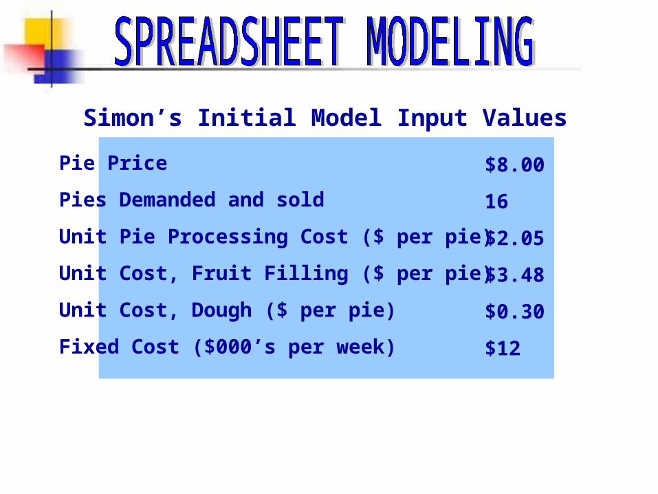
Simon’s Initial Model Input Values

Pie Price

Pies Demanded and sold

Unit Pie Processing Cost ($ per pie)

Unit Cost, Fruit Filling ($ per pie)

Unit Cost, Dough ($ per pie)

Fixed Cost ($000’s per week)

$8.00

16

$2.05

$3.48

$0.30

$12

To represent this model in an Excel Spreadsheet,you should adhere to the following recommendations:

Present input variables together and label them.

Clearly label the model results.

Give the units of measure where appropriate.

Store parameters in separate cells as data and refer to them in formulas by cell references.

Use bold fonts, cell indentations, cell underlines and other Excel formatting options to facilitate interpretation.

Initial Simon Pie Weekly Profit Model

(Click on spreadsheet to open Excel)

“ What if?” ProjectionAllows you to determine what would happen if you used alternative inputs.

For example, what would the resulting Profit be if the Profit for Pie Price and Pies Demanded changed to $7.00 and 20,000 or $9.00 and 12,000, respectively.Simply change the values of these parameters in the spreadsheet to view the resulting Profit.

What if we change the values of two parameters?

What effect will that haveon Total Cost and Profit?

Refining the ModelAfter reviewing the results, Simon has determined that this model treats the variables Pie Price and Pies Demanded as if they were independent of each other. Knowing this is not the case, Simon developed the following mathematical (linear) relationship:

Pies Demanded = 48 – 4 * Pie Price ($0 < price < $12)

Demand as a function of Price

01020304050

0 2 4 6 8 10 12

Pie Price

Pie

De

ma

nd

Refining the ModelNow, modify the spreadsheet to include this relationship. Keep in mind that the physical results should be separated from the financial or economic results.

More “What if?”You can copy the model into adjacent columns and change specific values in order to compare and contrast the changes.

More “What if?”Using Excel’s Chart Wizard, the resulting changes can be graphed in an X-Y Scatter plot for viewing.

Note that Profit is largest at a Pie Price of about $9.00 and that the break-even point of zero occurs at about $6.25.

Sensitivity AnalysisExamines what happens to one variable (usually a performance variable) when you change the values of another variable (usually an input variable).

For example, examine the effect of a percentage change in Pie Price on the percentage change in Profit.

Now you can use trade-off analysis to determine how much of one performance measure (Profit) must be sacrificed to achieve a given improvement in another performance measure (Pies Demanded & Sold).

Example 2: Simon Pie RevisitedSimon suspects that the previous model’s Processing Cost formula produces the correct historical cost for the base case of 12 thousand Pies Demanded, but not for other values of Pies Demanded. Validate the model by using actual Processing Cost data for different levels of pie production.

Use Excel’s Trendline capability to fit a trend equation directly to the actual cost data.

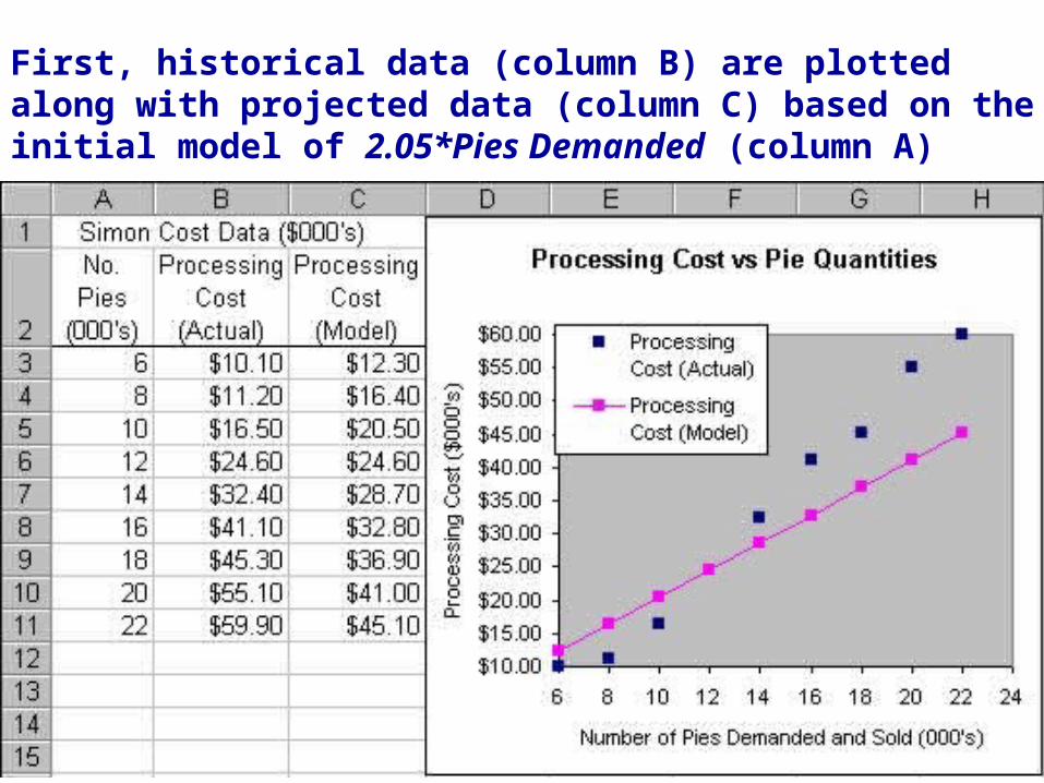
First, historical data (column B) are plotted along with projected data (column C) based on the initial model of 2.05*Pies Demanded (column A)

Next, right-click on the Processing Cost (Actual) series in the graph and choose the option Add Trendline.

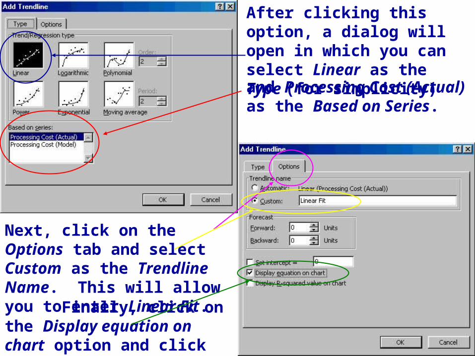
After clicking this option, a dialog will open in which you can select Linear as the Type (for simplicity)

and Processing Cost (Actual) as the Based on Series.

Next, click on the Options tab and select Custom as the Trendline Name. This will allow you to enter Linear Fit. Finally, click on the Display equation on chart option and click OK.

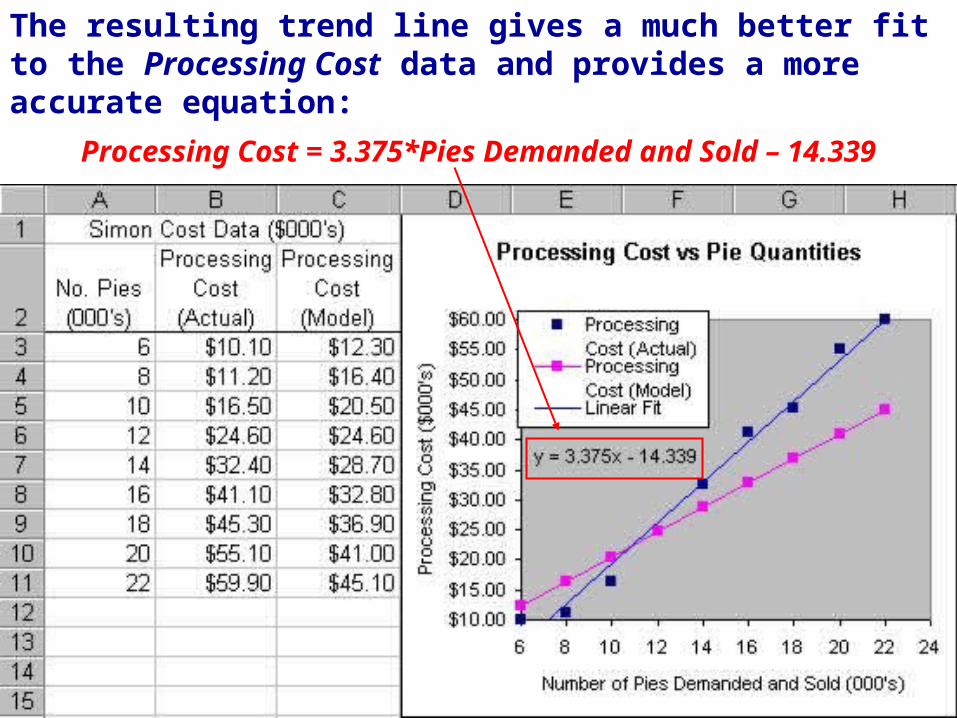
The resulting trend line gives a much better fit to the Processing Cost data and provides a more accurate equation:

Processing Cost = 3.375*Pies Demanded and Sold – 14.339

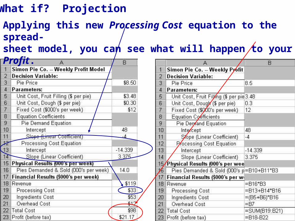
“ What if?” Projection

Applying this new Processing Cost equation to the spread-sheet model, you can see what will happen to your Profit.

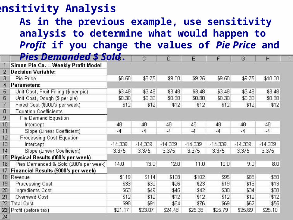
Sensitivity AnalysisAs in the previous example, use sensitivity analysis to determine what would happen to Profit if you change the values of Pie Price and Pies Demanded $ Sold.

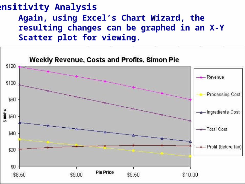
Again, using Excel’s Chart Wizard, the resulting changes can be graphed in an X-Y Scatter plot for viewing.

Sensitivity Analysis

Printing and Displaying the Spreadsheet ModelsNote that you can print and display these spreadsheet models such that technically oriented parameters can be hidden from higher level management reports.

To do this, highlight the desired rows

and then click on the

Data pull down menu and choose the Group and Outline –

Group option.

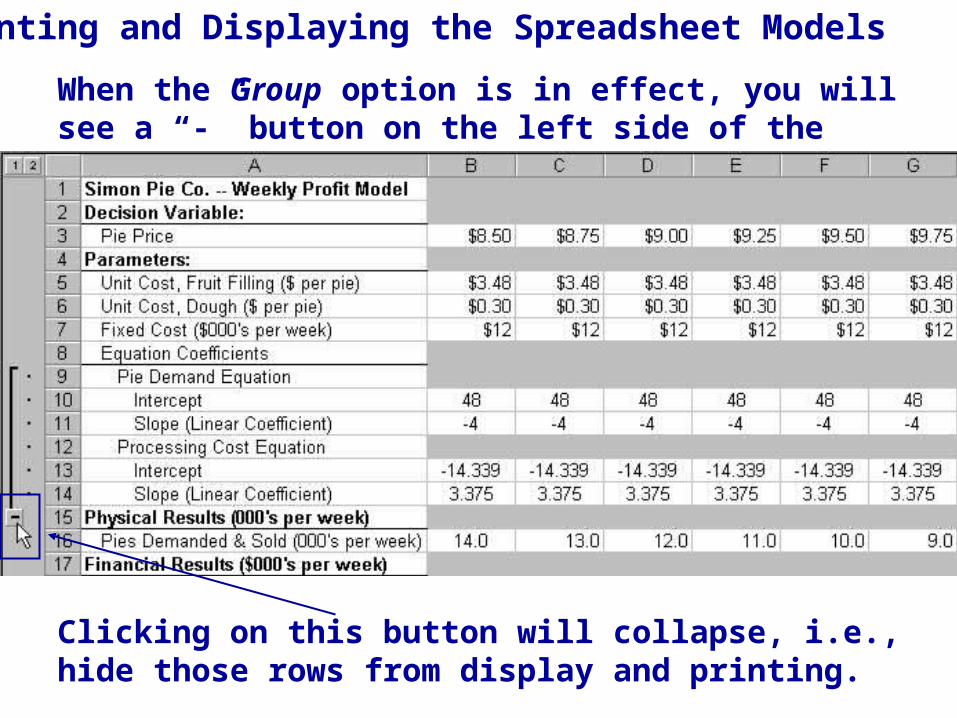
Printing and Displaying the Spreadsheet Models

When the Group option is in effect, you will see a “-” button on the left side of the spreadsheet.

Clicking on this button will collapse, i.e., hide those rows from display and printing.

Printing and Displaying the Spreadsheet Models

While in this “hide” mode, a “+” button will be displayed on the left side of the spreadsheet.

Clicking on this button will reveal the rows for modeling and analysis.

NOTE: Collapsing cells which comprise a data series in an Excel chart will temporarily remove the series from the chart.

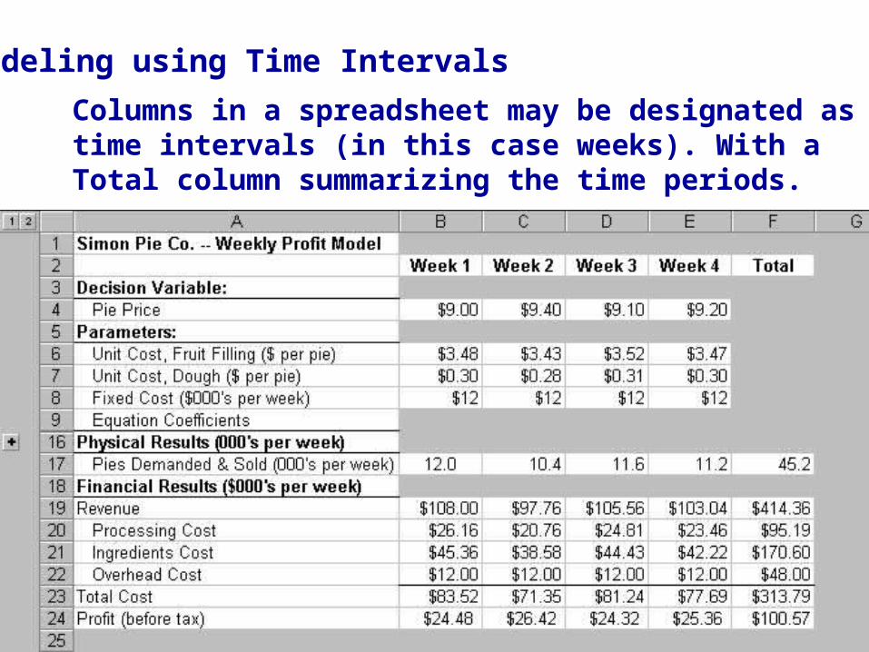
Modeling using Time Intervals

Columns in a spreadsheet may be designated as time intervals (in this case weeks). With a Total column summarizing the time periods.