Decision Mining in ProM: From Log File s to DMN Decision...
95
UNIVERSITEIT GENT GHENT UNIVERSITY FACULTEIT ECONOMIE EN BEDRIJFSKUNDE FACULTY OF ECONOMICS AND BUSINESS ADMINISTRATION ACADEMIC YEAR 2015 – 2016 Decision Mining in ProM: From Log Files to DMN Decision Logic Masterproef voorgedragen tot het bekomen van de graad van Master’s Dissertation submitted to obtain the degree of Master of Science in Business Economics Master of Science in Business Engineering Samuel Peeters Under the guidance of Prof. F. Gailly
Transcript of Decision Mining in ProM: From Log File s to DMN Decision...
UNIVERSITEIT GENT
GHENT UNIVERSITY
FACULTEIT ECONOMIE EN BEDRIJFSKUNDE
FACULTY OF ECONOMICS AND BUSINESS ADMINISTRATION
ACADEMIC YEAR 2015 – 2016
Decision Mining in ProM: From Log Files to DMN Decision Logic
Masterproef voorgedragen tot het bekomen van de graad van
Master’s Dissertation submitted to obtain the degree of
Master of Science in Business Economics Master of Science in Business Engineering
Samuel Peeters
Under the guidance of
Prof. F. Gailly

ii
Faculty of Economics and Business Administration
Academic Year 2015–2016
Decision Mining in ProM:
From Log Files to DMN Decision Logic
Samuel Peeters
Promotor: Prof. dr. F. Gailly
Thesis for the degree of
Master of Science in Business Engineering: Operations Management

PERMISSION
I declare that the content of this Master’s Dissertation can be consulted and/or reproduced
if the sources are mentioned.
Gent, 17 May 2016
S. Peeters

Preface
The writing of a thesis is never a simple task, but this one in particular could never have
materialized without the help and support of a number of people.
Of course, I have to thank Professor Gailly for suggesting this very interesting subject, but
also for talking some sense into me when I was getting lost in the many possibilities that a
broad subject like this one offers.
Steven Mertens deserves a lot of praise for the time he took to give me guidance, the many
good suggestions he made and the excellent humor during our meetings, making this stressful
period a little bit more bearable.
Special thanks to Eric Verbeek, who helped me get going on the plug-ins when the technica-
lities of the ProM structure were still mystifying to me.
The many researchers affiliated with the Eindhoven University of Technology made this paper
possible with their myriad and impressive contributions to the field of process and decision
mining.
My friends, for giving me confidence and teaching me to expect more of myself. My parents,
for making me who I am and allowing me the luxury of a great education. My girlfriend,
Lauranne, for keeping me centered, supporting me in all my endeavors and changing my
perception of what’s important.
Samuel Peeters
Gent 17 May 2016
iii

iv

Abstract
The field of process mining – the automated extraction of information on processes based on
event logs – has recently brought forth a number of publications on decision mining, which
concerns the automated extraction of the decision rules governing the routing decisions in the
process. While significant advances have been made in this regard, little to no attention has
been given to the manner of presentation of the decision logic that is discovered. This greatly
reduces the utility for daily practice of existing decision mining implementations. Decision
Model and Notation (DMN) is a new standard for decision modeling, which could be used to
tackle this problem.
This paper assuages the issue of lacking presentation of discovered decision logic by developing
and presenting a set of plug-ins for the popular ProM framework, which can mine, construct,
visualize and export DMN-compliant decision tables from log files in a user-friendly fashion.
This entails a significant improvement in the presentation of the decision logic discovered by
decision miners.
v

vi

Table of Contents
List of Figures ix
1 Introduction 1
2 Background and Related Work 5
2.1 ProM . . . . . . . . . . . . . . . . . . . . . . . . . . . . . . . . . . . . . . . . 5
2.2 Workflow: From Log Files to Decision Logic . . . . . . . . . . . . . . . . . . . 9
2.3 Logging and Log File Formats . . . . . . . . . . . . . . . . . . . . . . . . . . . 10
2.4 Process Mining . . . . . . . . . . . . . . . . . . . . . . . . . . . . . . . . . . . 12
2.5 Decision Mining . . . . . . . . . . . . . . . . . . . . . . . . . . . . . . . . . . . 21
2.6 DMN . . . . . . . . . . . . . . . . . . . . . . . . . . . . . . . . . . . . . . . . 27
2.7 Absence of Clear Presentation of Decision Logic in ProM . . . . . . . . . . . 33
3 Research Question 35
3.1 Scope . . . . . . . . . . . . . . . . . . . . . . . . . . . . . . . . . . . . . . . . 36
4 Research Methodology 39
5 Implementing DMN Decision Tables in ProM 6 43
5.1 Requirements . . . . . . . . . . . . . . . . . . . . . . . . . . . . . . . . . . . . 43
5.2 Implementation . . . . . . . . . . . . . . . . . . . . . . . . . . . . . . . . . . . 44
5.3 User Guide . . . . . . . . . . . . . . . . . . . . . . . . . . . . . . . . . . . . . 47
6 Evaluation 53
7 Conclusion and Future Work 65
Bibliography 69
A Definitions 75
B Generating Log Files 77
vii

Table of Contents viii

List of Figures
2.1 The ProM 6 package manager. . . . . . . . . . . . . . . . . . . . . . . . . . . 7
2.2 The object manager screen in ProM 6. . . . . . . . . . . . . . . . . . . . . . . 8
2.3 A BPMN model of the decision mining workflow. . . . . . . . . . . . . . . . . 9
2.4 UML class diagram for the XES standard. . . . . . . . . . . . . . . . . . . . . 12
2.5 Three types of process mining. . . . . . . . . . . . . . . . . . . . . . . . . . . 13
2.6 The BPM life-cycle. . . . . . . . . . . . . . . . . . . . . . . . . . . . . . . . . 14
2.7 The quality dimensions of a process model. . . . . . . . . . . . . . . . . . . . 17
2.8 Simplified representation of the logic behind a genetic algorithm. . . . . . . . 20
2.9 A BPMN model of a very basic claims handling process. . . . . . . . . . . . . 22
2.10 The decision tree view in the ProM 5 Decision Miner. . . . . . . . . . . . . . 24
2.11 An example of the output of the DataPetriNets Miner. . . . . . . . . . . . . . 25
2.12 An overview of the framework proposed in de Leoni et al. (2014). . . . . . . . 26
2.13 DMN decision notation. . . . . . . . . . . . . . . . . . . . . . . . . . . . . . . 29
2.14 DMN input data notation. . . . . . . . . . . . . . . . . . . . . . . . . . . . . . 29
2.15 DMN business knowledge model notation. . . . . . . . . . . . . . . . . . . . . 29
2.16 DMN knowledge source notation. . . . . . . . . . . . . . . . . . . . . . . . . . 29
2.17 An example decision requirements diagram (DRD) . . . . . . . . . . . . . . . 30
2.18 The BPMN - DMN link. . . . . . . . . . . . . . . . . . . . . . . . . . . . . . . 31
2.19 Example of a boxed expression. . . . . . . . . . . . . . . . . . . . . . . . . . . 31
2.20 Elements of a decision table. . . . . . . . . . . . . . . . . . . . . . . . . . . . . 32
4.1 The design science framework. . . . . . . . . . . . . . . . . . . . . . . . . . . 39
5.1 The matrix displaying the various rules in the resulting DMN table. . . . . . 45
5.2 An overview of the possible workflows through the new package. . . . . . . . 46
5.3 Importing a log file. . . . . . . . . . . . . . . . . . . . . . . . . . . . . . . . . 48
5.4 Selecting a plug-in in the action tab. . . . . . . . . . . . . . . . . . . . . . . . 48
5.5 The Petri net discovered by the Alpha Miner. . . . . . . . . . . . . . . . . . . 49
5.6 The first settings page for the decision miner. . . . . . . . . . . . . . . . . . . 49
5.7 The second settings page for the decision miner. . . . . . . . . . . . . . . . . 50
ix

List of Figures x
5.8 The third settings page for the decision miner. . . . . . . . . . . . . . . . . . 51
5.9 The DMN Decision Table visualizer. . . . . . . . . . . . . . . . . . . . . . . . 51
5.10 Examples of exported decision tables. . . . . . . . . . . . . . . . . . . . . . . 51
6.1 Simplified CPN process model used to generate log file for case 1. . . . . . . . 55
6.2 DMN Decision Table Visualizer for case 1. . . . . . . . . . . . . . . . . . . . . 55
6.3 DMN Decision Table for case 1 exported in HTML/CSS. . . . . . . . . . . . . 56
6.4 DMN Decision Table for case 1 exported in FEEL expressions. . . . . . . . . 56
6.5 Simplified CPN process model used to generate log file for case 2. . . . . . . . 57
6.6 DMN Decision Table Visualizer for case 2. . . . . . . . . . . . . . . . . . . . . 57
6.7 DMN Decision Table for case 2 exported in HTML/CSS. . . . . . . . . . . . . 58
6.8 DMN Decision Table for case 2 exported in FEEL expressions. . . . . . . . . 58
6.9 Simplified CPN process model used to generate log file for case 3. . . . . . . . 58
6.10 DMN Decision Table Visualizer for case 3. . . . . . . . . . . . . . . . . . . . . 59
6.11 The output of the exporters for case 3. . . . . . . . . . . . . . . . . . . . . . . 59
6.12 Simplified CPN process model used to generate log file for case 4. . . . . . . . 60
6.13 DMN Decision Table Visualizer for case 4. . . . . . . . . . . . . . . . . . . . . 60
6.14 The output of the original DPN Miner for case 4. . . . . . . . . . . . . . . . . 61
6.15 The output of the exporters for case 4. . . . . . . . . . . . . . . . . . . . . . . 61
6.16 Simplified CPN process model used to generate log file for case 5. . . . . . . . 61
6.17 DMN Decision Table Visualizer for case 5. . . . . . . . . . . . . . . . . . . . . 62
6.18 The output of the exporters for case 5. . . . . . . . . . . . . . . . . . . . . . . 62
6.19 Simplified CPN process model used to generate log file for case 6. . . . . . . . 63
6.20 DMN Decision Table Visualizer for case 6. . . . . . . . . . . . . . . . . . . . . 63
6.21 The output of the exporters for case 6. . . . . . . . . . . . . . . . . . . . . . . 63
7.1 Comparison of presentations of decision logic. . . . . . . . . . . . . . . . . . . 66
Chapter 1
Introduction
The growing popularity in the business world of ERP-systems and other Process Aware
Information Systems (PAIS) that are used to support, manage and control business processes,
has resulted in a veritable explosion of data concerning the execution of these processes. This
data is contained within these systems and in the log files1 they generate as output or which
can be created based on this data.
A wealth of information concerning the processes is hidden inside these logs, the exploitation
of which could be advantageous to the businesses that have generated them. While the logs
are by definition based on the execution of a process, the structure and attributes of this
underlying process aren’t necessarily explicitly known by the business.2
The logs can be studied from a number of perspectives (van der Aalst (2011); de Leoni et al.
(2016)):
• Control-flow perspective: The ordering of the various activities in the process. This is
the focus of process mining3, which results in a process model, and will be discussed in
section 2.4.
• Data-flow perspective: Various attributes attached to events or process instances and
how they are used and altered throughout the process. Decision mining (cf. section
2.5) can be seen as part of this perspective, as it studies how these data attributes (and
other information) influence which routing is followed through the process.
1A number of important terms for this paper are defined in appendix A.2In contrast with what the name suggests, not all PAIS’s have an explicit notion of the underlying process.
Only modern Business Process Management (BPM) and Workflow Management (WFM) systems can claim to
incorporate this (de Leoni & van der Aalst (2013)).3The term ’process mining’ is used in the narrow sense throughout this paper, i.e. the discovery of the
process model, of which the traces contained in the log files are instances. When talking about process mining
in the broad sense, i.e. extracting any type of knowledge on the underlying process from log files based on
executions thereof, this will be explicitly mentioned.
1
Chapter 1. Introduction 2
• Organizational perspective: What organizational resources (this includes employees)
are assigned to particular cases or activities.
• Time perspective: This perspective uses the timestamps contained within logs to dis-
cover bottlenecks, predict remaining time in a process execution, etc.
• Conformance perspective: Once a process model has been discovered or a normative
process model has been put forward, process instances can be compared to this model
to study conformance.
All of this has spawned a healthy field of research on how to extract and utilize this know-
ledge, starting in the late 90’s with Cook & Wolf (1998) in the context of analyzing software
engineering processes (Werner & Gehrke (2013)).
The majority of this research concerns algorithms that focus on discovering control-flow, i.e.
utilizing data mining techniques to discover the different activities in a process, the gateways,
and the pathways between them (de Leoni et al. (2013)).
Process models that are the result of this process mining process (e.g. a BPMN model), give
an overview of the possible paths through the process, but don’t give an indication of what
situations lead to a particular path being taken. This is the subject of decision mining, which
analyses the log files to discover the rules governing the decision points in the process model.
So far, most research in the field of decision mining has focused on the performance of the
proposed algorithms, leading to implementations that have a less than stellar user interface
and output the discovered decision logic in a way that isn’t optimal for real-world applications.
This is in contrast with the growing attention for visualization within the broader data-
mining-community, which is an indication of the importance for daily practice of proper
representation of information. A recent standard called Decision Model and Notation (DMN)
(Object Management Group (OMG) (2015)) has provided a clear way forward in this regard,
as it offers a standardized way of displaying this decision-related information to end-users in
a transparent way.
This paper aims to fix this lack of proper representation of the results of decision mining by
developing a user-friendly way to extract and display decision logic in a clear way within the
popular open-source ProM framework for process mining. More specifically, a set of plug-ins
will be created to mine and display DMN-compliant decision tables within ProM and export
these in a number of formats to facilitate sharing of the discovered decision logic.
The remainder of this paper is structured as follows.
Chapter 2 starts by presenting the ProM framework, followed by a short explanation of the
workflow that this paper aims to complete, i.e. how to go from log file to properly displayed
decision logic. Next, the various parts of this workflow will be covered individually. Special
attention will be given to the importance and advantages of these various subjects for daily

Chapter 1. Introduction 3
practice, in addition to giving an overview of the current state-of-the-art of these subjects, in
particular as implemented within the ProM framework. In chapter 3 the research question of
this paper is presented, followed by the methodology that will be used to tackle it (chapter 4).
The paper then moves on to discuss the actual implementation (chapter 5) and an evaluation
thereof based on a number of cases (chapter 6). Chapter 7 rounds off the paper with a
conclusion and suggestions for future work.

Chapter 1. Introduction 4

Chapter 2
Background and Related Work
2.1 ProM
This section introduces the ProM framework. It first positions it in the field of available
process mining solutions, followed by a short history of the framework. Finally, an overview
is given of the types of plug-ins and the features that make it one of the most popular process
mining solutions currently available.
All of the process mining theories, algorithms and standards that will be mentioned in the
following sections need to be implemented into a user-friendly product before they can be of
any use to the business world.
While commercial solutions do exist, such as SAP process mining by Celonis1 and Disco by
Fluxicon2, these are usually limited in functionality, more often than not to process discovery,
process visualization and some conformance checking functionality (cf. infra).
ProM is an open-source, Java-based framework that attempts to resolve this. It is a central
application that can be extended with context aware plug-ins and enjoys a large support
from the scientific community.3 The many plug-ins that are currently available4 have made it
the most complete process mining application available to date, incorporating functionality
covering all parts of the process mining spectrum, i.e. process discovery, conformance and
enhancement (cf. section 2.4), as well as data preprocessing.
The original version of the ProM framework was developed by researchers at the Eindhoven
University of Technology in 2004 in order to integrate the efforts of the various researches
affiliated with this institution. Version 1.1 was later introduced to the public in 2005 by
1http://www.sap.com/pc/tech/business-process-management/software/process-mining/index.html2https://fluxicon.com/disco/3The paper that introduced the framework to the broad public (van Dongen et al. (2005)) has close to 600
citations according to Google.4The central repository for these plug-ins can be found at https://svn.win.tue.nl/trac/prom/browser/Packages.
5
Chapter 2. Background and Related Work 6
van Dongen et al. (2005) and quickly gained support, leading to a substantial growth in the
number of available plug-ins. While version 1.1 could be used with only 29 plug-ins, by the
time version 4.0 was released in 2007 more than 140 plug-ins were available (van der Aalst
et al. (2007)). That number has grown to exceed 500 since then.
As research progressed and more plug-ins became available, the framework became unruly
and hard to maintain. After a final release based on the original code base, version 5.2, a new
version of the framework was written from the ground up, culminating in ProM 6 (introduced
by Verbeek et al. (2011)), which also introduced support for the new XES-standard for log
files (cf. section 2.3).
The plug-ins for the ProM framework are divided into categories:
• Discovery plug-ins: These take a log file as input and return a specific type of model.
Examples include the Heuristic miner and the α-algorithm Miner.
• Conformance checking plug-ins: These check conformance between a given model and
log files based on the same process. Examples include the plug-in to check the confor-
mance of log to a Petri net with data.
• Enhancement plug-ins: These take a log file and a process model as input and try
to enhance the given model by extracting additional insights from the logs that were
provided. At least, this is the definition that is given by ProM. It seems that a plug-in
enhancing log files with additional attributes has also received this designation, though
it doesn’t comply with the definition.5
• Filtering plug-ins: These provide the user with the functionality to filter elements or
cases out of a given log or to cluster the log, which can be useful for differentiated
analysis. An example is the plug-in that allows the user to filter out a random number
of events from a log, for example to test the robustness of an algorithm.
• Analytic plug-ins: These perform various types of analysis on a given log. An example
is the plug-in to analyze BPMN models.
• Input/output plug-ins: These allow the importing and exporting of various objects (e.g.
different types of process models, (altered) logs, Petri net markings, etc.) to and from
the application (no surprises here).
Besides these categories, one could also consider the visualizers for various types of objects
as a separate category.
On some occasions, the categorization is less than straightforward. E.g. the miner for Petri
nets with data is marked as a discovery plug-in, while it would be considered an enhancement
5It should be noted that plug-in developers are responsible for assigning one or more categories to their
plug-in, which might be a source of inconsistencies.

Chapter 2. Background and Related Work 7
plug-in according to many sources (e.g. (van der Aalst (2011), p. 216)) as it takes both a
log file and a process model as input and returns an identical process model which has been
enhanced with information that has been extracted from the log file (in this case additional
information on the data-flow). Another example are the plug-ins that convert a process model
of a certain type into another type (e.g. EPC’s to Petri nets). These don’t really find a correct
category within this taxonomy.
Besides the fact that it is open-source, ProM has a number of features that make it attractive
to both business users and the scientific community, including some that especially developers
of plug-ins will appreciate.
• A clear GUI and a library of reusable visual elements for the plug-ins: This allows for
easier interaction with the application, thus lowering the learning curve. The library
makes sure6 that the plug-ins have a similar look and feel as the central elements of the
framework, making the whole feel more like a single, well-developed application instead
of a combination of loose elements.
• An integrated package manager: This makes it easy to find and install plug-ins, in
addition to keeping them up to date automatically. It furthermore guarantees that
dependencies are in order, allowing the plug-ins to be smaller in size.
Figure 2.1: The ProM 6 package manager.
• An object manager: Objects that were loaded into the application or were created by
a plug-in, such as process models and logs, are kept in a list within the application as
long as it remains open. This removes the need to reload different files for every step in
the user’s workflow.
6It is up to the developer to choose if he uses these visual elements or not, but mostly they do. The range
of visual elements that ProM supports are one of the major limiting factors during plug-in development. More
on that in section 5.2.

Chapter 2. Background and Related Work 8
Figure 2.2: The object manager screen in ProM 6.
• Context aware plug-ins: Annotations within a plug-in’s code tell the framework what
types of objects it requires as input and what types of objects the framework can expect
as output. The central application uses this information to either present the user with
a list of plug-ins that can be used with one or more selected input objects, or to present
the user with a list of possible objects (based on the list in the object manager) that
can serve as input to a selected plug-in.
• Connections between objects: The ProM framework features a construct called ’connec-
tions’. These are a class of objects (usually hidden to the user) that serve as memory for
the links between different objects. They will for example remember that a particular
Petri net is linked to a specific log file because it was discovered using a specific miner
plug-in, while also storing the parameters that were used during this mining process.7
This makes it easier to see the links between different objects after the fact and allows
for reproduction of the steps. It also allows some plug-ins to complete their task in less
time, as they use information stored in these connections to gather already available
information that they would otherwise have recalculated themselves.
• Division between plug-in logic and user-interface: This makes the plug-ins easier to
maintain for the developers and also allows for headless execution of the plug-in (and
in some cases execution by means of distributed computing) whenever the developer
implemented this option.
• Possibility of automated workflows: The combination of context aware plug-ins and
possibility of headless execution allows for the creation of automated workflows by strin-
ging a number of plug-ins together. This is implemented in the companion application
7It is up to the plug-in developers to define these connections and what information they store.

Chapter 2. Background and Related Work 9
RapidProM8, which was introduced by Bolt et al. (2015) and is currently on version
3.0.
• Compatibility with data from a large array of enterprise applications: While the world
of log files – especially those coming from enterprise applications – suffers from a lack
of standardization, ProM’s companion application XESame allows extraction of log
information and conversion to ProM’s native XES-format for a large number of popular
applications and formats (cf. section 2.3).
2.2 Workflow: From Log Files to Decision Logic
This section presents the different steps that need to be taken in order to extract DMN-
compliant decision logic from log files within the ProM framework. It is this workflow that
will be completed by this paper. An overview of this process can be seen in figure 2.3.
Figure 2.3: A BPMN model of the decision mining workflow.
The process starts with the gathering of the required data. These are the log files, which
either came in a format ProM can understand or were extracted and converted to such a
format by means of XESame (cf. section 2.3) or similar tools (e.g. Fluxicon’s Nitro, which
has now been integrated into their Disco application). From here on out, the heavy lifting is
performed by ProM itself. Next up is the creation of a process model by means of process
mining (discussed in section 2.4). This model and the logs serve as input for the subsequent
decision mining phase, where the decision logic is discovered (cf. section 2.5) and which itself
entails a number of steps.9
8The name is a wordplay on the popular application RapidMiner, which allows for the creation of similar
workflows, but for more general data mining.9In most cases, steps 3 and 4 are covered by an algorithm that tackles a classification problem.

Chapter 2. Background and Related Work 10
1. Identification of decision points.
2. Identification of case routings in the log file, i.e. linking instances of the process to a
certain decision output.
3. Identification of variables relevant for a particular decision point.
4. Identification of cutoff-points and values for the variables that point to a particular
decision.
The final step is to present the results of the decision mining – the discovered decision logic – to
the user, preferably in an intuitive and standardized notation such as DMN. This functionality
is currently not adequately available within ProM. This paper will attempt to alleviate this
shortcoming by introducing a set of plug-ins to mine, convert and present decision logic in
the form of DMN decision tables (cf. infra).
2.3 Logging and Log File Formats
This section first inspects how data can be gathered for process and decision mining in the
ProM framework and then takes a closer look at the XES format for log files and what
information exactly can be contained within logs adhering to this format.
Process mining of course starts with the gathering of the data required by the process miner,
i.e. log files. These files contain information on a number of previous instances of the pro-
cess, usually referred to as cases or traces. These cases are in turn comprised of a sequence
of activities or events, and possibly additional attributes for these activities/events and/or
attributes at the case level.10
Today’s enterprise applications generate a deluge of useful data, but are also marked by a
complete lack of standardization of this data and the formats in which it can be exported from
these systems. Extracting the required information is frequently one of the largest hurdles to
overcome in process mining projects11 and one that is frequently ignored in literature. While
a number of plug-ins exist that allow the user to load different input formats, ProM 6 was
built with the XES log format in mind.
As was mentioned in section 2.1, the developers of the ProM framework have managed to get
around this issue by developing XESame, a companion application for ProM, which allows
for the extraction of relevant data from various enterprise applications and databases, as well
as the conversion thereof to the XES format, and the conversion of various other formats to
XES.12
10Taking it even further, XES allows nested attributes, i.e. attributes of attributes.11For an overview of some issues concerning the extraction of event logs, see (van der Aalst (2011), p113).12XES is the spiritual successor of the venerable MXML format. A similar conversion application, called

Chapter 2. Background and Related Work 11
XES (Gunther & Verbeek (2014)) is an XML-based format for log files that was developed in
order to advance standardization in log files and to resolve the shortcomings of the MXML
format that had been the closest thing to an accepted standard for log files up to that point.
The first version of the standard definition was released to the public in 2009, followed by
adoption of the standard by the IEEE Task Force on Process Mining in 2010.13 Version 2.0
of the standard was published in 2014 and added i.a. support for list and container attribute
types.
The main idea behind XES is to make it simultaneously as flexible and simple as possible,
allowing it to express a broad range of information on processes with a very limited number
of concepts.
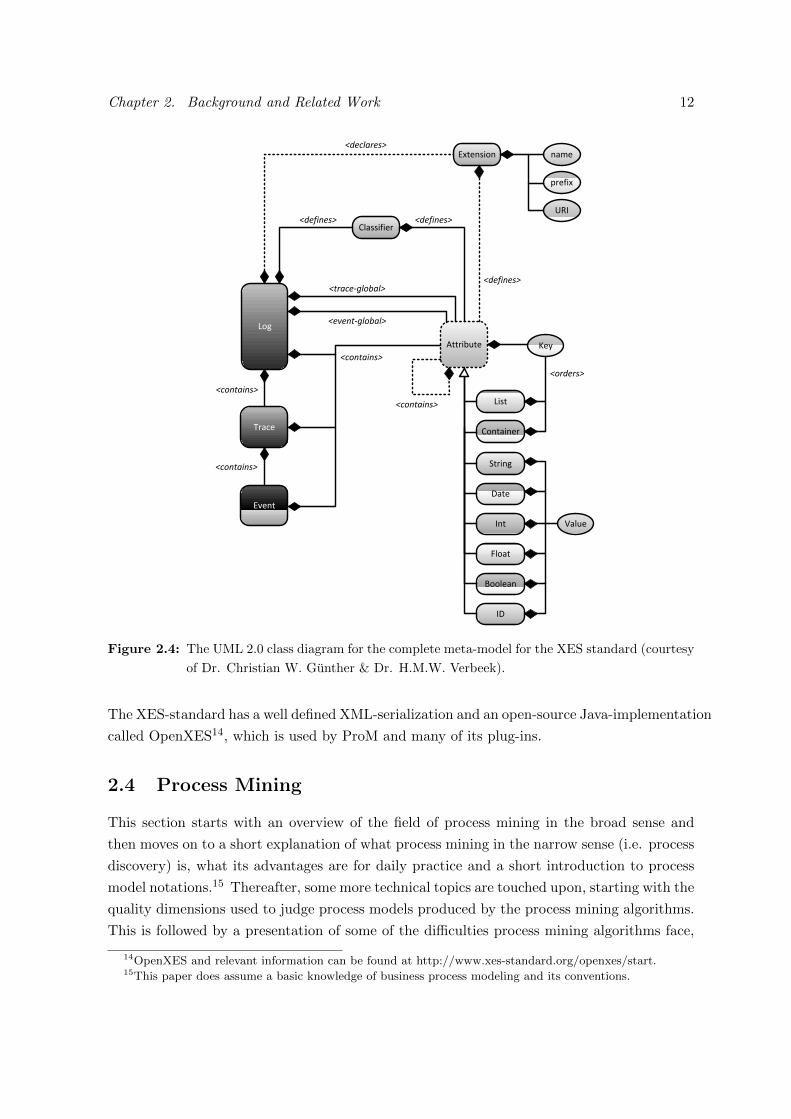
An overview of the standard as a UML diagram can be seen in figure 2.4. The main elements
are logs, which contain traces (process instances) of events. All of these can contain attributes
(key-value pairs), which can be nested. A short description of the most important features of
XES follows.
• Extensions: XES splits the retention of data from the semantics behind this data. The
concept of extensions allows for these semantics to be added to particular attributes,
allowing for interpretation of the data. This is achieved by having the log file point to
an external XESEXT-file. Attributes that utilize semantics from a particular extension
are preceded by the prefix linked to this extension. An example is the Organizatio-
nal extension, which defines attributes that can be used to express the organizational
resource(s) attached to an activity.
• Classifiers: In order to define which events are to be considered as being equal (i.e.
instances of the same activity), one or more event classifiers can be added to the log
files. These contain a list of event attributes. If two events have the same values for
these attributes, they are considered equal with regard to that classifier. The most
common example is events that have the same value for the concept:name-attribute.
• Global attributes: Declaring global trace or event attributes in the log makes these
attributes mandatory for every every trace, respectively event contained in the log. The
declaration of the global attribute contains a default value in case the attribute’s value
isn’t defined during log file generation.
• Typed attributes: An XES-attribute is always clearly typed, this in contrast with the
MXML-standard. Possible types are: String, Date, Int, Float, Boolean and ID. In addi-
tion there are lists, which hold any number of ordered child attributes, and containers,
which do the same, but in an unordered fashion.
ProMimport existed for this format.13The latest proposal for the standard can be found at http://www.xes-standard.org/xesstandardproposal.
Chapter 2. Background and Related Work 12
Log
Trace
Event
Float
Int
Date
String
Container
List
Attribute
Classifier
Extension name
prefix
URI
Key
Value
<declares>
<defines> <defines>
<defines><trace-global>
<event-global>
<contains>
<contains>
<contains>
<contains>
ID
Boolean
<orders>
Figure 2.4: The UML 2.0 class diagram for the complete meta-model for the XES standard (courtesy
of Dr. Christian W. Gunther & Dr. H.M.W. Verbeek).
The XES-standard has a well defined XML-serialization and an open-source Java-implementation
called OpenXES14, which is used by ProM and many of its plug-ins.
2.4 Process Mining
This section starts with an overview of the field of process mining in the broad sense and
then moves on to a short explanation of what process mining in the narrow sense (i.e. process
discovery) is, what its advantages are for daily practice and a short introduction to process
model notations.15 Thereafter, some more technical topics are touched upon, starting with the
quality dimensions used to judge process models produced by the process mining algorithms.
This is followed by a presentation of some of the difficulties process mining algorithms face,
14OpenXES and relevant information can be found at http://www.xes-standard.org/openxes/start.15This paper does assume a basic knowledge of business process modeling and its conventions.

Chapter 2. Background and Related Work 13
and a selection of process miners that have been implemented in ProM.16 This section is
rounded off by some thoughts on the importance of BPMN and its support within the ProM
framework.17
In (van der Aalst (2011), p. 216) process mining in the broad sense is divided up into three
main categories: process discovery (i.e. process mining in the narrow sense, which will be
covered in this section), conformance checking, and enhancement.18 This third category
enhances existing process models by extracting additional information on the process outside
the realm of control-flow from log files. Decision mining, which will be presented in section
2.5, is situated in this third category. An overview of this view on process mining in the broad
sense can be seen in figure 2.5.
Figure 2.5: Three types of process mining.
Process mining in the narrow sense, also called process discovery, is the first category in this
taxonomy. It is the construction of a process model based on information contained in log
files without any a priori knowledge on the underlying process. It takes as input a log file
and returns a process model that is representative of the control-flow behavior seen in the log
(van der Aalst (2011)).
Within the BPM cycle (cf. figure 2.6) process mining can be situated at the process discovery
16In depth information on the inner workings of these miners is beyond the scope of this paper. Some
excellent monographs on this subject are available, e.g. (van Dongen et al. (2009)).17For an extensive overview of process mining in the broad sense and related topics, see (van der Aalst
(2011)).18Some might also include data preprocessing as an additional category

Chapter 2. Background and Related Work 14
phase.19 Conventionally, this phase would be done manually or with the help from modeling
tools, but in the case of process mining it is performed in an automated fashion by means of
algorithms.
Figure 2.6: The BPM life-cycle.
Numerous advantages of process mining can be discerned for daily practice. Some are specific
for process mining and some can be linked to a good process discovery in general.
• More accurate process discovery: Automated process discovery removes the normative
and subjective factor from the equation. Instead of a modeling of the process done by
people who are involved in the process and might be biased by a normative perspective
on the process (i.e. they know what it should look like in principle and want to make the
reality look better than it actually is) or done by people who may not be familiar with
the process and thus need to rely in information that can be incomplete or is provided
by the people mentioned before, the process modeling is now done by an objective
algorithm that bases itself solely on information generated by previous instances of the
process, i.e. the process in reality.
• Better conformance checking: Modeling of the process (i.e. process discovery in the
19The second category in the process mining taxonomy, conformance checking, can be situated in the process
monitoring & control phase.

Chapter 2. Background and Related Work 15
BPM life-cycle, cf. figure 2.6) - the more accurate, the better - allows for a more
objective detection of cases (instances of the process) that deviate from the norm. This
is already the case for manual process modeling, but automated modeling based on
previous (successful) instances ensures that the model fits reality more closely, thus
signaling real aberrant behavior when deviations from that model are detected. All of
this allows for faster and more accurately detection of problems, thus reducing potential
negative effects.
• Delta analysis: Discovering what the process looks like in reality allows the business to
compare this actual process with a prescriptive process model, i.e. ’how it should be’
(van der Aalst et al. (2004)).
• Documentation and standardization: Documenting the process by developing a process
model of it is the staring point for the standardization of the process, which can be
advantageous in many situations, e.g. for obtaining certain certifications.
• Starting point for process analysis and improvement/redesign: In order to study a
process, analyze its performance and identify improvements, the process first needs to
be understood as it currently exists, which is exactly what process mining and process
discovery in general facilitate with the process models they have as output. Based on
the process model, further analysis methods, such as simulation, can be applied in order
to pinpoint bottlenecks and other problems, as well as opportunities for improvement.
• Improved communication: Having a visual and well-defined process model facilitates
communication and discussion about the process, e.g. during training of new employ-
ees. This is especially the case when these models are expressed in well-understood
and intuitive modeling languages such as BPMN. These languages define a shared vo-
cabulary, which reduces ambiguity when talking about the models and their underlying
processes.
Process models come in many shapes and sizes.20 There are a number of popular modeling
languages/notations, which can be roughly divided into those that have well defined formal
semantics such as process algebras (Baeten & Weijland (1990)), Petri nets (Petri (1966)) and
YAWL (van der Aalst & ter Hofstede (2005)) on the one hand, and those that have less formal
semantics, but tend to be more intuitive, such as BPMN (Object Management Group (OMG)
(2014)) and EPC’s (van der Aalst (1999)). The former are popular in research, whereas the
latter are preferred by business users (Lohmann et al. (2009)). The exception to this rule
seems to be YAWL, which has gotten interest from both ’sides’ (Lohmann et al. (2009)).21
20http://workflowpatterns.com/evaluations/ contains systematic comparisons of the features of a wide range
of notations.21For a comparative study on the popularity and key characteristics relevant for the use of different modeling
languages, see (De Weerdt et al. (2015), p532-534).

Chapter 2. Background and Related Work 16
Recently there has been a lot of interest for constraint-based modeling languages, such as
DECLARE (Pesic et al. (2007)), which are much more flexible than the ’traditional’ notations
and allow for modeling of more loosely structured processes. This falls outside the scope of
this paper.
Most process mining algorithms produce a Petri net or a variant thereof as output. However,
for real-world use BPMN (Business Process Model and Notation) is by far the most dominant
process model notation. Conveniently, Petri nets can be converted to BPMN models, as well
as to BPEL models and UML Activity diagrams (cf. infra).
The remainder of this paper will be largely based on Petri nets wherever a process model is
required, although BPMN models will be briefly touched upon later in this section.
Process models that are the result of process mining can be judged by a number of quality
dimensions, which describe the quality of the match between the process, the behavior captu-
red in the log and that described by the discovered process model (cf. figure 2.7). In general,
there is a trade-off between the following four quality dimensions (Werner & Gehrke (2013)).
• Fitness: Behavior captured in the log should fit within the boundaries set up by the
process model. In case of perfect fitness, every succession of events that occurs in the
log is also a possible succession of activities in the discovered process model.
• Simplicity: The output of the algorithm should be the simplest possible process model
that is able to explain the general behavior contained in the log (cf. Occam’s Razor).
E.g. a model containing each possible succession of activities separately will have perfect
fitness, but will not be the simplest model of the behavior that is observed in the process.
• Precision: The discovered model shouldn’t allow for behavior that diverges too far from
that which is observed in the logs. The model should not allow for too much behavior.
• Generalization: The model should be a presentation of all possible behavior of the
underlying process, not just the example behavior contained in the log files. This has
to do with avoiding overfitting of the model.
Discovering a process model that scores well on these dimensions is never a trivial task. A
number of challenges are salient within the field of process mining (van der Aalst et al. (2012)).
Take notice of the links that these challenges have with the different quality dimensions and
the balancing between the quality dimensions that is required as a result of these challenges.
• Representation bias: The choice for a particular modeling language that will serve as
the basis for the output of the miner inherently imposes limitations on what can be
discovered, as every language has its assumptions. This is what is called the ’represen-
tation bias’. A good example of this is the difference between rigid languages such as
Petri nets and those that allow for more flexible modeling such as DECLARE. Mining

Chapter 2. Background and Related Work 17
Figure 2.7: The quality dimensions of a process model.
a complex, flexible process to a Petri net, will produce unsatisfactory or overly com-
plex results. The choice for a modeling language (and thus for a particular miner, as
these are usually linked) should be driven by these constraints, not by an affinity for a
particular representation.
• Incompleteness: While most examples given in literature are fairly simple in order to
get the point across, real-life processes are frequently much more complex, comprising
a multiple of the amount of activities comprised in those examples. This leads to a
plausible situation where not all behavior that is possible in the process is reflected in
the log files for these real-world processes. Algorithms such as the α-algorithm work
around this by utilizing a different notion of completeness than the global one (i.e. all
beginning-to-end successions of activities are represented in the log). Instead of looking
at a complete end-to-end succession, it considers possible successions between just two
activities (this is the notion of ’completeness of direct succession’ ).22
• Noise: Within the context of decision mining, the concept of ’noise’ can either mean
faulty event data in the logs or exceedingly rare or exceptional behavior data. The latter
can lead to so-called spaghetti models, which aren’t wrong per se, but are so complex
that they lose much of their usefulness. This problem is usually tackled by a threshold
on the support and confidence metrics. Successions of activities that score too low on
the support metric (e.g. an exceptional situation that occurs in less than 1% of the cases
of a log, pointing to either a vary rare situation in the process or a case of erroneous
logging) aren’t withheld for the final process model. Within this context, the notion
exists of the 80/20 model. This suggests that for most cases, it is best to aim for a model
that describes 80% of the behavior seen in the log, as this behavior can be explained by
a model that is only 20% of the model required to describe all behavior (Leemans et al.
(2014a)), and the remaining 20% causes 80% of the variability in the process (van der
22For a complete overview of different notions of completeness, see (van Dongen et al. (2009), p228).
Chapter 2. Background and Related Work 18
Aalst (2011), p148). This leads to a simpler, clearer model of the central behavior of
the process.
• More technical challenges: Elements such as loops, hidden tasks (tasks that are not
captured in the log file, but should be present in the process model), and duplicate
activities (multiple activities with the same name/label in one process, which can be
either separate tasks or the same task performed at different stages (cf. call activities
in BPMN)) can in many cases confound process mining algorithms or are difficult for
them to support (van der Aalst et al. (2003)).
Over time, algorithms that were able to tackle the issues discussed above were developed.23
There are currently a number of excellent algorithms available in ProM, each with its own
strengths and specializations (e.g. the Heuristics Miner, which specializes in handling noisy
logs).
Some of the most frequently mentioned algorithms are presented here.24
• The α-algorithm: One of the oldest process mining algorithms, developed in 2004 by
van der Aalst et al. (2004). It has been implemented in ProM 6 by means of the Alp-
haMiner package.
This deterministic algorithm starts by recording all the different successions of events
present in the log file. Based on this, more advanced orderings are created (e.g. exclu-
sive choice splits), and finally these advanced orderings are used to construct the final
model.25 These three phases are called abstraction, induction and construction, and
can be seen in many algorithms.
This algorithm has its limitations. For example, it can’t differentiate between short
loops and true parallelism. Furthermore, α-algorithm has issues dealing with noise (in
the sense of low-frequency behavior) and incompleteness in the log (van Dongen et al.
(2009), p234). Many extensions of this algorithm have been constructed in order to
compensate for these limitations, e.g. the α+-algorithm, which isn’t thwarted by short
loops (de Medeiros et al. (2005)). It has also led to the development of more advanced
algorithms.
• HeuristicsMiner algorithm: This algorithm was postulated in 2003 by Weijters & van der
Aalst (2003), but wouldn’t be implemented until 2006, when it was introduced as a ProM
plug-in (Weijters et al. (2006)). It takes a log file as input and produces a heuristic net
23In some cases, an algorithm wasn’t enough to solve the complications. This was the case for complex,
flexible and loosely coupled processes, which simply couldn’t be adequately represented in the traditional
modeling languages. This led to the development of the DECLARE language, which falls outside the scope of
this paper.24An excellent comparison of different process mining algorithms that had been developed by 2009 can be
found in (van Dongen et al. (2009)).25For a detailed description of the inner workings of this algorithms, see (van der Aalst (2011), p129-156).
Chapter 2. Background and Related Work 19
as output, which is a variant of a causal net. This algorithm was developed with noise
and incompleteness in mind. It does this by not just looking into the possible successions
of activities, as the α-algorithm does, but also at the frequency of these successions (i.e.
support). Because of this, it is better suited to mine the main behavior of a process
(cf. 80/20 model). It also supports all common constructs in process models, such as
loops, choice and parallelism, with the exception of duplicate activities (van Dongen
et al. (2009), p235).
• Fuzzy Miner: A variant of the HeursticMiner algorithm introduced by Gunther &
van der Aalst (2007). It gives even further control over the level of abstraction by
introducing additional user-specified parameters and multiple log-based process metric
used to determine the correct level of detail in the final process model. For example,
less significant, but highly correlated behavior is clustered and hidden in subprocesses,
leading to a hierarchical, clear process model. It is implemented in ProM by means of
the Fuzzy package and produces a so-called fuzzy model. This algorithm is also the
basis for the commercial process mining solution Disco by Fluxicon.26
• Genetic algorithm: Taking a cue from optimization theory, adaptations of evolutionary
algorithms were developed for application in process mining. In contrast to the pre-
vious algorithms, these introduce an aspect of randomness to the mining process, thus
reducing reproducibility.
The most famous of these adaptations is that of the genetic algorithm, which was im-
plemented in ProM by de Medeiros et al. (2007) in the EvolutionaryTreeMiner package.
This plug-in once again has a Petri net as output. It is based on traditional genetic
algorithms (Eiben & Smith (2003)) that mimic nature by working with different ge-
nerations of gene pools, constructing descendants thereof (which are constructed by a
process termed crossover), which may or may not have mutations in their ’DNA’, and
using ’survival of the fittest’ to determine who will make it to the next ’generation’
by assigning a fitness value to these descendants (in addition to keeping the ’fittest’
examples of the previous generation around, which is termed elitism). A simplified
representation of this algorithm can be seen in figure 2.8.
This algorithm supports all common constructs, while simultaneously being able to
handle noise and incompleteness in logs.
• Inductive Miner: A more recent addition to the process mining cannon, this algorithm
was introduced in 2013, with an updated version to better deal with infrequent behavior
presented shortly thereafter by Leemans et al. (2014a).27 It was implemented in ProM
with the InductiveMiner package. It’s main advantage is that it guarantees to produce
26http://fluxicon.com/blog/2012/05/say-hello-to-disco/27This paper also includes a nice comparison of existing miners with special attention for soundness of the
resulting models.

Chapter 2. Background and Related Work 20
Figure 2.8: Simplified representation of the logic behind a genetic algorithm.
sound models (e.g. free of deadlocks), while handling noise with ease and being generally
efficient.
• DECLARE Miner: Based on the approach proposed by Maggi et al. (2011), this plug-in
allows the mining of a DECLARE model. It allows the user to specify what kind of
DECLARE templates they are interested in, resulting in a more exact control over the
discovery process.
It’s quite striking that most of these mining algorithms have Petri nets (or extensions thereof,
such as Petri nets with inhibitor arcs and/or reset arcs) or other very formal languages and
notations as the format of the process models that they produce.28 This is mainly because
these semantically sound languages are popular in the research community. However, busi-
ness users mostly prefer more intuitively understood languages and notations such as BPMN,
which sadly doesn’t easily lend itself to mining.
Recently, steps have been taken to fix this discrepancy within the ProM framework between
available miners and demand from the business world. This by means of conversion methods
between Petri nets and BPMN models, and a miner for BPMN models.
Kalenkova et al. (2014) first described the BPMN capabilities of ProM as a response to this
discrepancy. The solution they presented was to use a combination of well-established process
miners for other notations and plug-ins that allowed for the conversion of these other types
28Other output formats of process mining algorithms include heuristic nets (Weijters et al. (2006)), causal
nets (van der Aalst et al. (2011)), and EPC’s (Dumas et al. (2005)).

Chapter 2. Background and Related Work 21
of models (Petri nets, causal nets and process trees) to BPMN (and vice versa in the case of
Petri nets). BPMN support in ProM was already available by means of the BPMN package
and this paper introduced the BPMN Conversion package with the necessary converter plug-
ins.29
A process miner with native support for BPMN was introduced by De Weerdt et al. (2015).
It mines both the control-flow and organizational aspects (swimlanes) of the process. The
mining algorithm is robust to noise and is implemented in ProM in the BPMNMiner package.
This BPMN functionality in ProM is important, as it significantly increases the appeal for
users outside the scientific community, given the popularity of this standard. From the view-
point of business users, a version that outputs BPMN process models and a clear representa-
tion of the discovered decision logic would be the ideal incarnation of the workflow presented
in section 2.2.
2.5 Decision Mining
This section will first give a short introduction on different definitions of decision mining,
afterwards elucidates the advantages this has for daily practice and finally moves on to a
succinct chronological overview of the advances made in the field of decision mining (in ProM)
and a final remark on the output format of these miners.
Decision mining, also called decision point analysis, is the study of the decision-related charac-
teristics of a process based on a process model of the process and log files of previous process
executions. It enriches30 process models (focused on the control-flow of a process) with addi-
tional insights on why specific decisions are made (i.e. why is a specific routing through the
process taken) and in some cases also the circumstances surrounding this decision, e.g. when
in the process certain variables are defined and altered (de Leoni & van der Aalst (2013)), or
the organizational elements involved in the decision.31
Decision mining in the narrow sense (which is how this term is used throughout the remainder
of this paper) involves the automated discovery of the decision logic of decision points in the
process.32 Decision points are situations in a process where one or more options need to be
chosen from an array of possibilities. The decision logic for the these decision points represents
29Theoretical research on conversions between different modeling languages had been performed earlier, e.g.
(Lohmann et al. (2009)) and (Raedts et al. (2007)), but this was the first implementation of such functionality
in ProM.30This means that it is part of the third type of process mining in the categorization presented at the start
of section 2.4.31While this is an element of the decision model as defined by DMN (cf. section 2.6), the majority of
literature would classify this as being organizational mining (van der Aalst (2011); Song & van der Aalst
(2008)).32This difference between broader decision modeling and decision logic returns in the DMN specification,
which will be covered in section 2.6.

Chapter 2. Background and Related Work 22
the conditions that need to be fulfilled for a specific option to be taken. It is strongly related
to the data-flow of the process, as it requires determining what variables33 are relevant for
the routing decision (i.e. feature selection) and for what values34 of these variables a specific
routing is taken. E.g. in the very elementary claims handling process which can be seen in
figure 2.9, the value of the claim determines whether a basic analysis is performed or a more
in-depth analysis is required.
Figure 2.9: A BPMN model of a very basic claims handling process.
The modeling of this decision logic in general and doing so in an automated way in particular
has numerous advantages.
• All of the advantages mentioned for process modeling and mining in section 2.4 are also
valid for decision modeling and mining.
• Making implicit knowledge explicit: A lot of knowledge within an organization is tacit
and often concentrated in a few key people for a particular process. This is especially
the case where decisions need to be made. Externalizing this knowledge in the form of
decision logic and models is important for the sharing and diffusion of this knowledge
throughout the organization, as well as for the continuity in business processes (e.g.
when a key figure leaves the company).
• Precision fine-tuning of decision parameters: Only after the decision logic has been
mapped can the fine-tuning process start. Changing cutoff points and other parameters
can lead to improvements in efficiency, cost savings, reduction of rework, etc.
• Improved conformance checking: Involving decision logic in conformance checking can
greatly improve its performance, as it adds an entirely new and in many cases very
relevant dimension (Mannhardt et al. (2015b)). While a particular trace can seem
33Case and event attributes, but in some cases also other performance measures that aren’t readily available
in the logs and need to be calculated after the fact (Bazhenova & Weske (2015); de Leoni et al. (2016)).34Depending on the type of variable being studied, this can be a range, an inequality, etc.
Chapter 2. Background and Related Work 23
acceptable from a control-flow perspective, it may become clear that something is amiss
when also taking data-flow and in particular decision logic into account. This can be
particularly important in the context of fraud detection (e.g. unusual decisions in loan
granting processes).
• More efficient decision making and automation: Giving the discovered decision logic a
normative status allows for a more routine and straightforward decision making process
for the people involved. This leads to efficiency improvements in the form of a higher
volume of decision tasks being processed by the same amount of resources. An extension
of this would be the full automation of the decision task35, which is now possible as the
decision logic has been formalized.
• Reduction of uncertainty and variability: This same formalization and standardization
of decision rules leads to a reduction of uncertainty for the people involved, which in
turn can lead to a reduction of stress. Furthermore, it may decrease the variability in
the process, which is something every organization would welcome.
• Simplifying process models: Intricate decisions concerning multiple input variables and
many different options can sometimes lead to very large and extensive process models
being required to capture this logic (cf. a decision tree being captured in a process
model). Isolating decision logic from control-flow of a process can significantly reduce
the number of elements in a process model, thus increasing its clarity.
The field of decision mining has been marked by a succession of approaches, each one building
upon the previous. Issues such as loops in the process model and invisible tasks can now be
handled with ease by modern miners.36 A short chronological overview follows, with special
attention for implementations in the ProM framework.37
The chronology necessarily starts with the extensive research done on decision tree algorithms
and other machine-learning techniques (Mitchell (1997)), such as Bayesian Networks (Sutris-
nowati et al. (2013)), Markov Models (Lakshmanan et al. (2013)), Support Vector Machines
(Polato et al. (2014)), etc. This because mining for the decision logic behind a decision point
can in essence be reduced to a classification problem with the dependent variable being the
35I.e. the creation of independent decision services within the BPMS of an enterprise, replacing what used
to be a user-performed work task (the making of the decision).36The biggest issues for decision mining concern the correct interpretation of the control flow of the process,
which for example determines what the possible choices are in a particular decision. An overview of these
control-flow related difficulties can be found in (Rozinat & van der Aalst (2006a)).37While other, more general approaches to knowledge discovery in data exist (e.g. Mues et al. (2005);
Fayyad et al. (1996)), as well as scientific works that are counterparts to the ones discussed here, but aren’t
aren’t applied to ProM (e.g. Rozinat et al. (2006)), discussing these falls outside the scope of this paper.

Chapter 2. Background and Related Work 24
output/decision/routing. Many of the following algorithms either directly use or are based
upon open source algorithms like those found in the Weka library38.
Whereas some prior research on data-oriented process mining for specific problems existed
(e.g. Ly et al. (2006)) and for other systems (e.g. Grigori et al. (2004)), the first steps to
introduce a working decision miner for general purposes in the ProM framework were taken
by Rozinat & van der Aalst (2006b). The implementation in ProM 5 (cf. figure 2.10) of this
approach (aptly called the Decision Miner plug-in) takes a Petri net and MXML-logs as input
and utilizes the J48 decision tree classifier of the Weka library, itself an implementation of
the C4.5 algorithm (Quinlan (1993)) to determine the decision tree related to a particular
decision point. This first attempt at decision mining in ProM had serious limitations such
as not being able to deal with loops and invisible activities. Another limitation is that it
can only discover guards that conform to the structure: variable - equality or inequality -
constant. Despite these issues and the fact that the plug-in only exists for the outdated ProM
5 framework, this decision miner remains popular, even in recent studies such as (Bazhenova
& Weske (2015)).
Figure 2.10: The decision tree view in the ProM 5 Decision Miner.
The next major step in this evolution was the work proposed by de Leoni & van der Aalst
(2013) and implemented in ProM by means of the DataPetriNets package. The main focus
is on an extension of the Petri net convention called ’Petri nets with data’. This allows
the adding of read and write operations to the Petri net transitions, as well as the adding
of transition guard functions, i.e. logical expressions that need to evaluate to true before a
particular transition can fire. Other than this new data structure and the mining of additional
features, this contribution improved upon the previous Decision Miner by allowing process
models with loops and hidden activities to be properly mined. The implementation in ProM
38http://www.cs.waikato.ac.nz/ml/weka/.

Chapter 2. Background and Related Work 25
of the concepts proposed in this paper became the first functional decision miner in the new
and improved ProM 6 framework (cf. figure 2.11). Once more, the C4.5 algorithm was
used by the plug-in to build the necessary decision trees. Later on, this plug-in was reused
and integrated into the Multi-perspective Process Explorer plug-in for ProM (introduced by
Mannhardt et al. (2015a)), which provides an integrated environment for the user to analyze
and explore a given event log.
Figure 2.11: An example of the output of the DataPetriNets Miner.
The next contribution came from de Leoni et al. (2013). This extended existing decision
mining capabilities by allowing the mining of decision guards that contained arithmetic ope-
rations (e.g. x1 + x2 > 25). This was achieved by applying the Daikon system39 for discovery
of invariants and utilizing the output thereof as input for decision tree algorithms provided
by Weka. The techniques were implemented in the standalone application Branch Miner.40
The results were promising (although they came at a computational cost larger than other
algorithms), but there seemingly hasn’t been any follow-up research down this path.41
While all of the scientific contributions mentioned up to this point focused on one particular
aspect of extracting information from logs, i.e. process discovery, discovery of data-flow,
etc., de Leoni et al. (2014) puts forward a framework that allows one to look for correlations
between any type of data that can be read from or created based on log files. One could for
example try to predict the remaining time of the process instance based on various event-
attributes, or look into the correlation between the income of an applicant and his chances
39htpp://groups.csail.mit.edu/pag/daikon/dist/40http://sep.cs.ut.ee/Main/BranchMiner41Although traces of an implementation can be found in the DataPetriNets ProM package, development
thereof seems to have been abandoned.
Chapter 2. Background and Related Work 26
for being approved for a loan.42 Obviously, this framework could also be used to find the
attributes that correlate significantly with the taking of a particular path at a decision point,
i.e. decision mining. Another feature of this framework is its ability to enrich the provided log
files with ‘a broad and extendable set of characteristics related to control-flow, data-flow, time,
resources, organizations and conformance‘. Furthermore, a number of filters are provided to
control which events (and their associated attributes) are retained for analysis. In (de Leoni
et al. (2016)) this framework was extended to allow clustering of the log into sub-logs based on
previous analysis. This can be useful for many reasons, e.g. analyzing different clusters with
different algorithms more suited for their contents, or simply because discovering a different
process for each cluster leads to more user-friendly results. An overview of the resulting
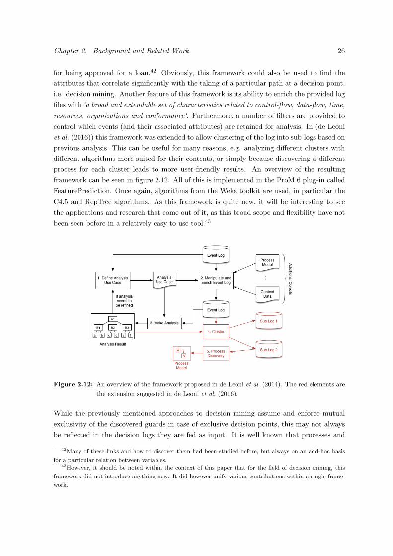
framework can be seen in figure 2.12. All of this is implemented in the ProM 6 plug-in called
FeaturePrediction. Once again, algorithms from the Weka toolkit are used, in particular the
C4.5 and RepTree algorithms. As this framework is quite new, it will be interesting to see
the applications and research that come out of it, as this broad scope and flexibility have not
been seen before in a relatively easy to use tool.43
Figure 2.12: An overview of the framework proposed in de Leoni et al. (2014). The red elements are
the extension suggested in de Leoni et al. (2016).
While the previously mentioned approaches to decision mining assume and enforce mutual
exclusivity of the discovered guards in case of exclusive decision points, this may not always
be reflected in the decision logs they are fed as input. It is well known that processes and
42Many of these links and how to discover them had been studied before, but always on an add-hoc basis
for a particular relation between variables.43However, it should be noted within the context of this paper that for the field of decision mining, this
framework did not introduce anything new. It did however unify various contributions within a single frame-
work.

Chapter 2. Background and Related Work 27
in particular their decision logic aren’t always that well-defined in reality, which can easily
lead to overlapping expressions for the different options coming out of a decision point that
is supposed to be an exclusive decision. An approach to decision mining that can cope with
this phenomenon is proposed by Mannhardt et al. (2016). It does this by adding a second
step after the growing of the initial decision tree, where the wrongly classified instances are
studied in depth to discover overlapping rules that alter the initial decision tree. Limited
validation of the approach was performed and while some improvements were detected for
the type of cases the algorithm was designed for, it is still possible that a deterioration of
performance could be present in other situations. This algorithm was implemented in ProM
by means of a new version of the Multi-perspective Process Explorer plug-in44 and once more
uses the C4.5 algorithm at its core.
Other lines of research to extend and improve decision mining (and process mining in general),
such as enriching event log data with domain specific semantic knowledge (cf. Jareevongpi-
boon & Janecek (2013)), have been established, but they exceed the scope of this paper.
The implementations of these approaches in ProM45 invariably take a Petri net as input.
One of the main drawbacks to using these plug-ins for real-world applications is that they
usually have (Petri net) transition guards as output. This is in contrast to the focus in
practical applications on entire decision points and their accompanying decision logic. In
most cases, the decision logic for a particular decision point can be obtained by combining
the guard expressions for the different transitions that start from the Petri net place that
represents that decision point. However, the situation does arise where multiple places lead
into the same transition. In this case it is impossible to identify which part of the transition
guard is linked to which decision point.
In general, the decision logic that is extracted by currently available miners is returned in
very unclear formats (cf. figure 2.11 and 6.14), thus significantly reducing the utility of these
plug-ins for daily practice. This is in contrast to the growing attention for visualization of
data in the wider data-mining field. Ameliorating this situation is the central focus of this
paper.
2.6 DMN
Many of the advantages mentioned in sections 2.4 and 2.5 are rooted in the shared under-
standing of the resulting models and the improved communication about these that is result
44Meaning that it was introduced in the DataPetriNets-package which this process explorer uses for decision
mining-related tasks.45Some aren’t implemented in ProM, but have been developed as standalone applications, e.g. Branch
Miner.

Chapter 2. Background and Related Work 28
thereof.46 This is of course contingent on a shared vocabulary and well understood notations.
For process models in the workplace, BPMN has largely fulfilled this role, but up to this point
no equivalent existed for the field of decision modeling (Taylor et al. (2013)).47
The introduction of the Decision Model and Notation standard (DMN) by the Object Mana-
gement Group (OMG) (2015) fills this void. The need for this type of standard is illustrated
by the large interest the modeling community has had for it in the short time since its release.
Authorities in the field such as Bruce Silver have published entire books on the subject (Silver
(2016); Debevoise & Taylor (2014)), an extension based on DMN of the popular declarative
process modeling language DECLARE was proposed (Mertens et al. (2015)) and popular
modeling tools such as Signavio48 and Camunda49 are quickly and enthusiastically adding
support for the standard.
This section will first give a succinct overview of DMN and then delves deeper into DMN
decision logic, in particular DMN decision tables, as these will be used extensively in the
solution that is presented in this paper to the problem of lackluster representation of the
output of decision mining in ProM.
DMN was introduced to provide a common language and notation that is readily understan-
dable by all business users, both for decision design/modeling and decision implementation.
It was designed to be useable alongside BPMN and provides semantics for decision models, a
standard visual language and an XML representation to support sharing of the models.
DMN consists of two distinct levels used to describe a decision and its context: the decision
requirements level and the decision logic level.50
The decision requirements level describes what will be decided, references the decision logic
that is required for making this decision and describes the interrelationships between decisions,
but doesn’t specify the actual rules that determine the output of the decision based on the
input (i.e. the decision logic). DMN uses four constructs in order to describe the decision
requirements level (section 6.2.1 of the DMN specification).
46The importance of thereof is stressed in ’The Process Mining Manifesto’ (van der Aalst et al. (2012)),
which explicitly mentions ’Improving understandability for non-experts’ as one of the main challenges for the
broader process mining field.47Catalkaya et al. (2014) made an attempt at creating just that, in the form of a variant of XOR-gateways,
called the r-gateway, which can contain decision rules. Other formats that are able to capture decision logic
do exist, e.g. Predictive Model Markup Language (PMML) (Grossman et al. (1999)) and Production Rule
Representation (PRR) (Object Management Group (OMG) (2009)), but these don’t cover the entire decision
model as DMN does. Furthermore, they aren’t as intuitively understood and they miss the compatibility with
BPMN.48http://www.signavio.com/news/managing-business-decisions-with-dmn-1-0/49https://camunda.org/50This division is analogous to the difference between broader decision mining and decision mining in the
narrow sense of discovering decision logic, as was discussed in section 2.5.

Chapter 2. Background and Related Work 29
Decision: The act of determining an output value from
a number of input values using a certain decision logic.
This corresponds to the business concept of an operati-
onal decision or a decision task (Taylor et al. (2013)).
Figure 2.13: Decision notation.
Input data: The data structures containing the values
needed to determine the output of the decision. They
describe the case about which decision are to be made.
The output of the decision can only depend on this input
data and the output of other decisions that are linked
to this decision in the decision model (cf. figure 2.17). Figure 2.14: Input data notation.
Business knowledge model: This denotes a function en-
capsulating business know-how in the form of business
rules, analytic models, or other formalisms. This know-
how comes down to decision logic that will convert in-
puts into decision outputs. By encapsulating it in the
concept of a business knowledge model this logic can be
reused by various decisions.Figure 2.15: Business knowledge
model notation.
Knowledge source: This concept designates autho-
rity for decisions or for business knowledge models.
Examples are source documents which define busi-
ness knowledge models, manuals or an expert res-
ponsible for making a particular decision.
Figure 2.16: Knowledge source notation.
Properly specifying and connecting51 these four elements results in what is called a decision
requirements graph (DRG), which can be visually represented in a decision requirements
diagram (DRD) (cf. figure 2.17).
The second level of DMN is the decision logic level, which describe how each decision’s outcome
is derived from its inputs in sufficient detail to allow validation and/or automation. The link
between input and output is unambiguous so that a particular set of inputs leads to the same
decision every time. DMN decision logic will be presented in-depth shortly.
Both levels, as well as the process model of the process containing the decision can be linked
51The relevant connection rules can be found in section 6.2.3 of the DMN standard specification.
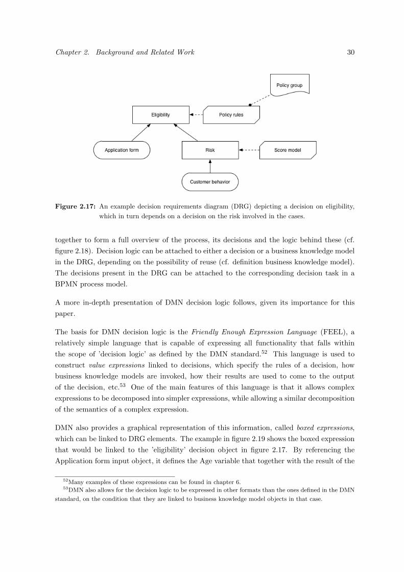
Chapter 2. Background and Related Work 30
Figure 2.17: An example decision requirements diagram (DRG) depicting a decision on eligibility,
which in turn depends on a decision on the risk involved in the cases.
together to form a full overview of the process, its decisions and the logic behind these (cf.
figure 2.18). Decision logic can be attached to either a decision or a business knowledge model
in the DRG, depending on the possibility of reuse (cf. definition business knowledge model).
The decisions present in the DRG can be attached to the corresponding decision task in a
BPMN process model.
A more in-depth presentation of DMN decision logic follows, given its importance for this
paper.
The basis for DMN decision logic is the Friendly Enough Expression Language (FEEL), a
relatively simple language that is capable of expressing all functionality that falls within
the scope of ’decision logic’ as defined by the DMN standard.52 This language is used to
construct value expressions linked to decisions, which specify the rules of a decision, how
business knowledge models are invoked, how their results are used to come to the output
of the decision, etc.53 One of the main features of this language is that it allows complex
expressions to be decomposed into simpler expressions, while allowing a similar decomposition
of the semantics of a complex expression.
DMN also provides a graphical representation of this information, called boxed expressions,
which can be linked to DRG elements. The example in figure 2.19 shows the boxed expression
that would be linked to the ’eligibility’ decision object in figure 2.17. By referencing the
Application form input object, it defines the Age variable that together with the result of the
52Many examples of these expressions can be found in chapter 6.53DMN also allows for the decision logic to be expressed in other formats than the ones defined in the DMN
standard, on the condition that they are linked to business knowledge model objects in that case.

Chapter 2. Background and Related Work 31
Figure 2.18: Example of BPMN process model and DMN DRG and Decision Logic linked together.
Risk decision serves as the input for the Policy rules, the business knowledge model that it
invokes and that supplies the output of the Eligibility decision.54
Figure 2.19: Example of a boxed expression.
One of the most important forms of boxed expressions is the decision table (defined in section
54Example borrowed from Taylor et al. (2013).
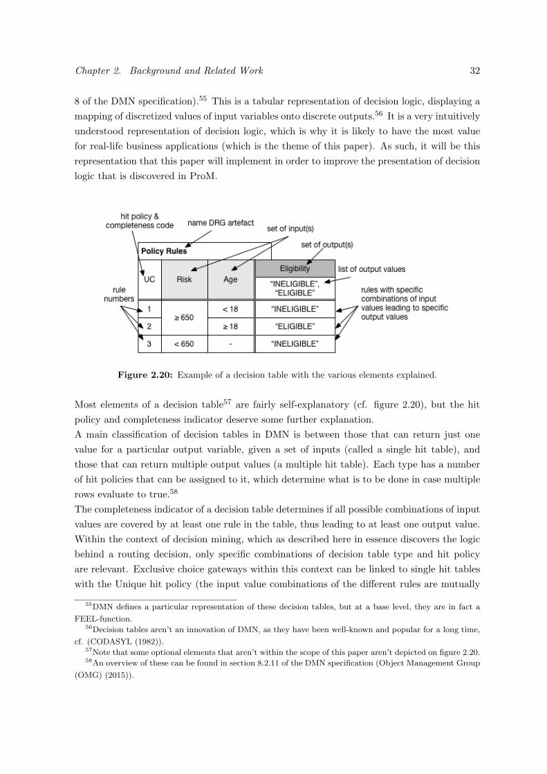
Chapter 2. Background and Related Work 32
8 of the DMN specification).55 This is a tabular representation of decision logic, displaying a
mapping of discretized values of input variables onto discrete outputs.56 It is a very intuitively
understood representation of decision logic, which is why it is likely to have the most value
for real-life business applications (which is the theme of this paper). As such, it will be this
representation that this paper will implement in order to improve the presentation of decision
logic that is discovered in ProM.
Figure 2.20: Example of a decision table with the various elements explained.
Most elements of a decision table57 are fairly self-explanatory (cf. figure 2.20), but the hit
policy and completeness indicator deserve some further explanation.
A main classification of decision tables in DMN is between those that can return just one
value for a particular output variable, given a set of inputs (called a single hit table), and
those that can return multiple output values (a multiple hit table). Each type has a number
of hit policies that can be assigned to it, which determine what is to be done in case multiple
rows evaluate to true.58
The completeness indicator of a decision table determines if all possible combinations of input
values are covered by at least one rule in the table, thus leading to at least one output value.
Within the context of decision mining, which as described here in essence discovers the logic
behind a routing decision, only specific combinations of decision table type and hit policy
are relevant. Exclusive choice gateways within this context can be linked to single hit tables
with the Unique hit policy (the input value combinations of the different rules are mutually
55DMN defines a particular representation of these decision tables, but at a base level, they are in fact a
FEEL-function.56Decision tables aren’t an innovation of DMN, as they have been well-known and popular for a long time,
cf. (CODASYL (1982)).57Note that some optional elements that aren’t within the scope of this paper aren’t depicted on figure 2.20.58An overview of these can be found in section 8.2.11 of the DMN specification (Object Management Group
(OMG) (2015)).

Chapter 2. Background and Related Work 33
exclusive, leading to just one rule evaluating to true for any given combination of input
values). Multi-choice patterns/OR gateways on the other hand, can capture their decision
logic in multi-hit tables, where the hit policy loses its relevancy in this context, as all outputs
will lead to a particular branch being followed, regardless of the order these outputs are
returned in (which is what the hit policy determines in this case).59
Regarding the completeness of decision logic discovered by decision mining, little can be said
in advance. This mostly depends on whether the full range of possible values of the input
variables is captures by the log file or if this range has been specified in some other way the
miner can understand.
2.7 Absence of Clear Presentation of Decision Logic in ProM
Contributions to the field of decision mining up to now have been primarily focused on various
performance aspects of the algorithms and less with how they would function in real-world
applications. In particular the presentation of the discovered decision logic to the user has
largely been forgotten.
As mentioned above, the existing plug-ins output decision guards for transitions instead of
decision logic for an entire decision point, thus moving even further away from the form factor
that is most intuitively understood en thus most useful in real-world applications.
While these things aren’t problematic for academic purposes, a full overview of the decision
logic for a decision point, in a clear and standardized notation does have many advantages
for daily practice (cf. supra).
An example of such a notation are the DMN decision tables. As DMN is a very recent
standard, it is understandable that not a single implementation thereof can be found in
ProM (although it is mentioned in Mannhardt et al. (2016)), but it does provide a clear
way forward with regard to the previously stated problem of the lacking representation of
discovered decision logic.
59For reference, the multiple hit policies are No order, Output order (a hierarchy of output values is defined
in the table), and Rule order (the order the rules are mentioned in the table).

Chapter 2. Background and Related Work 34

Chapter 3
Research Question
Up to this point, this paper has studied the possibility of going from log files to DMN decision
logic in an automated fashion within the ProM framework, along the way discussing various
related topics, in particular with the end-user in mind. The conclusion of this study was that
while extraction of decision logic is possible with certain ProM plug-ins, the framework is
currently lacking functionality that will also present this discovered decision logic in a clear,
standardized and user-friendly fashion, which is necessary to fully complete the workflow
presented in section 2.2. An example of such a clear presentation are decision tables, as
defined in the DMN specification.1
In order to introduce a user-friendly way of presenting discovered decision logic to business
users, this paper continues by posing the following research question:
Can DMN be utilized to extend an existing decision mining-algorithm within ProM in
order to enhance the produced output and the representation thereof, thus expanding its
utility for business-users?
The previous chapters should have established the importance of such user-facing functiona-
lity, in particular as a complement to the canon of research on decision mining, which up to
this point has been missing an interface that makes it useable for real-world business appli-
cations without an extensive background in the matter.
The ProM framework was chosen as the context for this question for many of the reasons
stated in section 2.1. Furthermore, its open-source and pluggable nature, combined with the
fact that ProM is currently one of the most prominent process mining (in the broad sense)
solutions give any artifact resulting from this endeavor a better chance of having an impact.
1Bazhenova & Weske (2015) recognizes this need and presents a similar workflow to the one discussed in
this paper, but transformation to DMN is performed manually.
35

Chapter 3. Research Question 36
3.1 Scope
A number of specifications and restrictions of the research question of this paper are in order.
These are split up in general specifications and restrictions and those specifically concerning
the output of the plug-in that will be developed as an answer to the research question.
• Perfect Petri nets as input: Up to now, no decision miner exists that utilizes another
format as input (cf. section 2.5). The miner will be supplied with a Petri net that
matches the control-flow of the process that lies at the base of the log files perfectly.
• Exclusive choice decisions as input: The main focus of this paper is on properly extrac-
ting and presenting DMN decision tables within the ProM framework. Testing mutual
exclusivity of the rules discovered by the decision miner is beyond the scope of this
paper. As DMN decision tables do require the specification of the hit policy, the plug-in
will always return a single hit table and specify the Unique hit policy (cf. infra) and
thus only input with decision points of the exclusive type will be supported.2 As a
result, only input of this type will be provided to the plug-in during testing.
• Decision miner performance disregarded: As the plug-in developed in this paper will
rely on an existing decision mining algorithm, the performance of this miner is outside
of the control of the author. The performance of the chosen miner has been studied in
the papers suggesting the methods it utilizes (cf. section 2.5) and as such no further
testing thereof will be performed.
A number of specifications on the output of the plug-in that is the subject of this paper follow.
Many of these are rooted in the fact that decision mining concerns a specific type of decision,
i.e. a routing decision through a process, which imposes a number of restrictions on the type
of decision tables that can be discovered.
• DMN 1.0: The last formal version of the DMN standard at the time of writing, ver-
sion 1.0 (Object Management Group (OMG) (2015)), will be used as a basis for the
implementation.
• Decision logic: Given the information that current decision miners discover (i.e. the
guards for Petri net transitions), this focus was inevitable. Constructing DMN DRG’s
would require the development of new miners or a novel combination of existing ones
(e.g. organizational miners to specify knowledge source objects).
• Decision tables: Given this paper’s focus on the end user, the intuitively understood
DMN-specified decision tables are the best DMN-conformant representation of the dis-
covered decision logic. The developed plug-in has to be able to display these tables
2Extension to other types of decision points is explicitly foreseen during development of the plug-ins and
a way forward will be presented in the chapter on future work (7).

Chapter 3. Research Question 37
clearly in the ProM framework, and export them both in a visible format, as well as in
the FEEL-expressions corresponding with the decision table.
• Focus on standard decision tables: Specific formats such as the cross-tab table (cf.
(Object Management Group (OMG) (2015), figure 8.8)) won’t be implemented. Only
horizontal tables will be supported, although implementing vertical tables would be
trivial at that point.
• Single output tables: As the studied decision are always routing decisions through a
process, there can only be one output variable, i.e. the route that will be taken. Multi-
output tables will thus not be incorporated.
• Single hit tables with the Unique hit policy: Given the earlier specification concerning
exclusive choice gateways, the discovered tables will always be of the single hit type
(i.e. only one output value is returned). This means that the discovered decision rules
should be mutually exclusive as well3, and thus that the hit policy will be Unique, as
current decision miners don’t support the discovery of decision logic for single hit tables
conforming to other hit policies.4
• Completeness assumed: The decision logic discovered by the decision miner is assumed
to be complete (i.e. covering the complete range of possible input values) and as such
no test for this is performed.5 As the completeness indicator is an optional attribute
of decision tables (Object Management Group (OMG) (2015), section 8.2.12), omitting
this from the final result wouldn’t detract from DMN-compliance.
3The discovery of overlapping rules in cases where the given Petri net specifies an exclusive choice has
been made possible within decision miners in ProM, but this results in inconsistencies between the discovered
decision logic and the underlying Petri net and as such will be disregarded.4Or this would require an algorithm that fuses different rows of a decision table together and defines
priority rules for the resulting rules. The parameters for this algorithm would be not very self-explanatory and
as such, the user-friendliness of the plug-in would be reduced, which is exactly what this paper wants to avoid.5This largely depends on the range of input values present in the traces of the log file. Creating a test for
this would require information on the range of possible values of these input variables, which is information
that is currently not available in log files.

Chapter 3. Research Question 38

Chapter 4
Research Methodology
As the research question is implementation oriented, the suitable research methodology for
this paper is design science.
Design science is defined as the research methodology geared toward the creation and eva-
luation of IT artifacts intended to solve identified organizational problems (Hevner et al.
(2004)).
Many methods, multi-step plans and frameworks have been suggested for this research me-
thodology.1 This paper will follow the methodology proposed by Peffers et al. (2007), in
the slight adaptation of Johannesson & Perjons (2014)2, because it provides both guiding
principles, as well as the steps required to perform such research.
Figure 4.1: The design science framework set forth in (Johannesson & Perjons (2014)).
1For an overview, see (Johannesson & Perjons (2014), p87-88).2This adaptation omits the ’communication’ step from (Peffers et al. (2007)), which is correct in the eyes
of the author as this step is inherent to all research.
39

Chapter 4. Research Methodology 40
As can be seen in figure 4.1, this framework consists of five sequential steps.
1. Explicate the problem: This phase requires an answer to the question:
”What is the problem experienced by some stakeholders of a practice and why is it
important?”
This step has been covered by the paper up to this point, based on the research method of
literature review that helped shape chapter 2 of this paper. This chapter illustrated the
advantages of decision modeling and mining, which have been established in existing
literature, as well as the advantages for daily practice linked to having a clear and
standardized notation for decision logic. As ProM is the most prominent and accessible
framework for process mining in the broad sense, the absence within this framework of
such a clear and standardized notation for presenting the results of decision mining can
be described as a problem3 warranting a solution.
2. Define requirements: The main question for this phase of design science is:
”What artifact can be a solution for the explicated problem and which requirements on
this artifact are important for the stakeholders?
The artifact in question will be a set of plug-ins to mine, construct, and display DMN
decision tables within the ProM framework. The requirements for these plug-ins will be
covered in section 5.1, which should be read in conjunction with the previous chapter
on the research question and its scope.
3. Design and develop artifact:
”Create an artifact that addresses the explicated problem and fulfills the defined require-
ments.”
This is where the actual creation of the design artifact takes place, in this case the
coding of the ProM plug-ins that implement DMN decision tables as an answer to the
research question. This will be covered in chapter 5.
4. Demonstrate artifact:
”How can the developed artifact be used to address the explicated problem in one or more
cases?”
The different steps required to operate the plug-ins will be illustrated in chapter 5, while
in chapter 6 the plug-in will be given a number of cases (i.e. generated log files and
accompanying Petri nets) in order to test how it performs in a variety of situations and
to illustrate how it provides a clear representation of decision logic.
5. Evaluate artifact:
”How well does the artifact solve the explicated problem and fulfill the defined require-
ments?”3A problem is sometimes defined as a gap between a desirable state and the current one, which is the case
here.

Chapter 4. Research Methodology 41
Chapter 6 will verify to what extent the requirements set out in the previous phases
have been achieved. This includes clarity of representation of decision logic, ease of use,
general applicability, and adherence to the DMN standard.

Chapter 4. Research Methodology 42

Chapter 5
Implementing DMN Decision
Tables in ProM 6
This chapter first covers the requirements for the package that will be developed and the
plug-ins that are contained by it, followed by a discussion of the implementation and the
challenges that were encountered during that implementation. Finally, section 5.3 presents a
user guide for the resulting package.
5.1 Requirements
This section should be read in conjunction with chapter 3, which defines much of the scope
of the plug-in1 that will be developed.
The plug-in should be able to provide the user with the following functionality:
1. Extract information needed to create a DMN-compliant decision table for a particular
decision point and present this in a DMN-compliant decision table notation, as specified
in section 8 of the DMN specification.
2. Export this decision table notation in a visual format that is easily shared.
3. Export the FEEL function that defines the decision table as specified in section 10.3.4.6
of the DMN specification to a text-file.
The plug-in should be able to provide this functionality without leaving the ProM framework
and regardless of the input that it is given, provided that the latter is within the scope set
out in section 3.1.
1Technically, the resulting artifact will be a ProM package, which contains a number of ProM plug-ins that
deliver the desired functionality. In this paper however, ’the package’ and ’the plug-in’ will mostly be used
interchangeably, as this is a technical distinction that is of little importance for what needs to be explained.
43

Chapter 5. Implementing DMN Decision Tables in ProM 6 44
Given the user-facing nature of this research question, ease of use will also be a major conside-
ration during the implementation. A minimum amount of the user’s time should be necessary
to extract the desired results.
5.2 Implementation
This section will cover only the non-trivial aspects of the implementation and the considera-
tions that led to particular design decisions. This will be done by walking through steps of
the plug-ins, mentioning interesting subjects when they are encountered.
First, the information necessary to construct the decision table for each decision point in the
process (or those that the user has chosen to mine) needs to be extracted.
As the purpose of this paper isn’t to develop a new decision miner, an existing one was cho-
sen as a basis for this step, namely the decision miner from the DataPetriNets package (DPN
miner from here on out). The choice for this package is rooted in the fact that it is actively
maintained, it has been proven to function (multiple papers have contributed to it and they
mention positive results (cf. section 2.5))2, various options and algorithms for mining are
implemented and the code is relatively well documented.
During testing of the developed plug-in, it became clear that the original DPN Miner contai-
ned an inconsistency that caused the mining process to fail when mining different processes
sequentially without restarting ProM. The source of this issue was tracked down and fixed.
DPN miner outputs the decision guards per transition in the Petri net. This means that it
merges guards linked to various decision points (i.e. in case multiple places that represent a
decision point lead to the same transition), as well as the different decision rules that lead to
the same transition in a particular decision point (i.e. when multiple decision rules in a single
decision point lead to the same decision/routing). As the separate decision rules, grouped
per decision point are needed in order to construct decision tables, the logic of the miner
needed to be changed in order to extract this information. The various function estimators
were altered to intercept the decision tree before it is converted to the output mentioned
above. From there it is converted to a new decision logic object. This object is also added to
the outputs that ProM expects from the plug-in. All this is done while keeping the original
functionality intact, so the user can enjoy the full range of functionality in a single package.
The new DecisionLogic object class contains the discovered rules, as well as the places and
transitions they are linked to. The choice was made not to convert the decision logic to DMN
decision tables at this point in order to accommodate potential future development of other
analyzers and visualizers of this data. The presence of the original places and transitions in
the object will allow for easy linking of the decision logic to the Petri net that was used as
2During testing, it came to light that this performance was exaggerated, or at least that big issues had not
been mentioned in these papers, cf. section 6.

Chapter 5. Implementing DMN Decision Tables in ProM 6 45
input for the miner.
Next, the information contained in the decision logic object (which can contain information
on multiple decision points) needs to be transformed into the various data fields required in
a DMN decision table. These include the decision name (in this case the name of the Petri
net place it is linked to), the different input variables that are present in the decision rules,
the possible output values (the names of the transitions), and the input entries. The latter
are the entries in the cells of the table (marked in bold in figure 5.1), which need to be in
the form of one of the DMN specified unary tests or a list of these type of tests, according to
section 9.5.3 of the DMN specification.3
Extracting this last bit information requires some parsing of the rules discovered in the pre-
vious step. Proper parsing allows for a much clearer visualization of the decision logic than
what is displayed by the original DPN Miner (cf. case 4 in chapter 6). One limitation that
is imposed on the input because of this parsing is that the attribute names and their values
can’t contain the following expressions: ==, !=, <, >, <=, >=, and &&.
Once the parsing is done, the matrix displaying the various rules in the table is constructed,
so every row contains a valid unary test for each input variable in the table.
A final step in the construction of the decision table is the joining together of different rules
where possible. This is the case when two rules with the same output value contain identical
conditions, save for one value of a nominal variable. Here, the two rules can be joined together
and the two values are joined into a list as specified by the DMN specification. An example
of this joining can be seen in figure 6.13.
The resulting decision table is contained in an object of the new class DecisionTables, which
is returned to ProM.
Figure 5.1: The matrix displaying the various rules in the resulting DMN table.
Considerations on ease-of-use and efficiency led to the creation of a couple of different plug-
ins, which ProM detects in the package.
Those who are interested in the output of the DPN Miner (i.e. the read and write operations
of data in the process and the guards as linked to the transitions), as well as the decision
3It should be noted that DMN allows for some flexibility in these expressions in the graphical version
of decision tables (cf. section 8.2.8 of the DMN specification). The design decision was made to employ
FEEL-specifications as much as possible.

Chapter 5. Implementing DMN Decision Tables in ProM 6 46
tables, will perform both previously mentioned steps (extraction of required information and
conversion thereof to decision tables) sequentially, by first calling the altered ’Discovery of
the Process Data-Flow (Decision-Tree Miner)’ -plug-in4, having a look at the output and then
calling the ’Convert Decision Logic to DMN Decision Tables’ -plug-in, which returns the final
DecisionTables object, to which ProM responds by automatically calling the new ’Show DMN
Decision Tables’ visualizer-plug-in that will be discussed shortly.
Those who just want to mine the decision tables and aren’t interested in the output of the
original DPN Miner can use the ’Discover DMN Decision Logic’ -plug-in, which integrates
both previously mentioned steps. It takes a Petri net and an accompanying log file as input,
asks the user to determine some options for the miner and returns a DecisionTables object
that ProM once again automatically visualizes by means of the ’Show DMN Decision Tables’ -
plug-in.
Figure 5.2: An overview of the possible workflows through the new package.
Once the DecisionTables object has been created, the decision tables contained within need
to be properly presented to the user in ProM. This is done by means of the ’Show DMN
Decision Tables’ visualizer-plug-in. This presents the DMN-compliant DMN tables in the
ProM design language, with a dropdown menu at the bottom that allows the user to flip
through the decision tables for the various decision points. This functionality is illustrated in
figure 6.17.
During the development of this step the age of the ProM framework became apparent, as only
JComponents can be utilized in visualizer plug-ins, while allowing for newer visual frameworks
such as JavaFX would have allowed the tables to be presented in a more attractive fashion.
A general remark on development of plug-ins for ProM would be that it is far from as easy
as literature presents it. There seems to be a general unwillingness to make negative remarks
about this framework that at times is misplaced.
4Out of respect for the original developers, the name of this plug-in wasn’t changed.

Chapter 5. Implementing DMN Decision Tables in ProM 6 47
Finally, the package should provide the user with the option to export the decision tables both
in a visible fashion, as well as in FEEL expressions (functionality 2 & 3). This is implemented
by means of the two export-plug-ins contained in the package.
For the visual exporter, a choice was made to export the visible representation of DMN
decision tables in HTML/CSS. This because as was mentioned in chapter 2, many of the
advantages of decision modeling and mining are related to easily understood notations that
can be readily shared. The choice for the intuitive representation of DMN decision tables
encapsulated in universally compatible HTML/CSS, maximizes the possibility of capturing
these advantages.
In all, six different plug-ins are provided in the developed package:
1. The altered ’Discovery of the Process Data-Flow (Decision-Tree Miner)’ -plug-in.
2. The ’Convert Decision Logic to DMN Decision Tables’ -plug-in.
3. The ’Discover DMN Decision Logic’ -plug-in.
4. The ’Show DMN Decision Tables’ visualizer-plug-in.
5. The export-plug-in that exports DMN decision tables in HTML/CSS.
6. The export-plug-in that exports DMN decision tables in their FEEL notation.
5.3 User Guide
In this section, a short step-by-step guide is given for the decision mining workflow as was
presented in section 2.2. As has been mentioned in the previous section, some of these steps
can be skipped depending on the needs of the user.
This guide assumes that ProM has been installed and the package has been added correctly.5
The user needs to make sure that the package ’RunnerUpPackages’ is installed by means of
the included package manager, as this is a dependency of DPN Miner, which is integrated
into the developed package.
After starting up ProM, you will be greeted by the workspace tab, which displays the objects
currently available to ProM. As this is empty at start-up, the log files that are to be mined
need to be loaded first by pressing the import button in the upper right corner and selecting
the log files. A number of import plug-ins will be suggested. Any starting with ’ProM log
files’ will load the desired object.
In order to check that no formatting errors occurred during the creation of the log and that
ProM imported it properly, it is prudent to check the data types of the attributes in the
5Information on how to do this is readily available online and OS-specific, so isn’t repeated here.
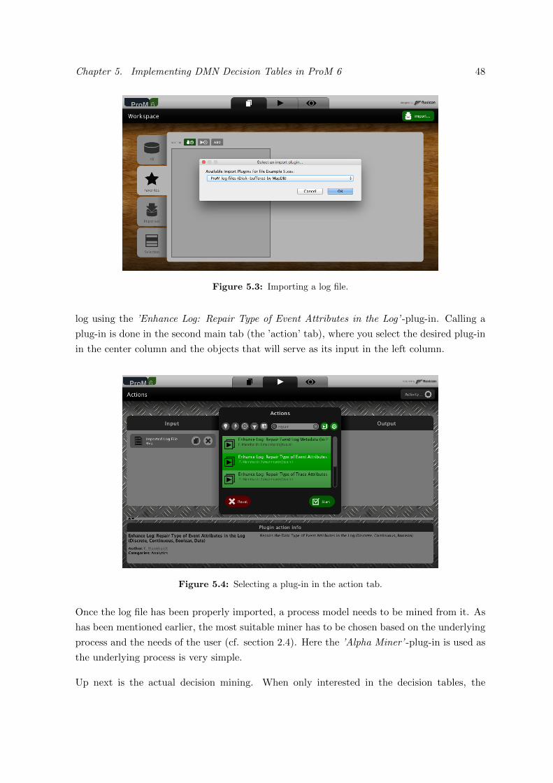
Chapter 5. Implementing DMN Decision Tables in ProM 6 48
Figure 5.3: Importing a log file.
log using the ’Enhance Log: Repair Type of Event Attributes in the Log’ -plug-in. Calling a
plug-in is done in the second main tab (the ’action’ tab), where you select the desired plug-in
in the center column and the objects that will serve as its input in the left column.
Figure 5.4: Selecting a plug-in in the action tab.
Once the log file has been properly imported, a process model needs to be mined from it. As
has been mentioned earlier, the most suitable miner has to be chosen based on the underlying
process and the needs of the user (cf. section 2.4). Here the ’Alpha Miner’ -plug-in is used as
the underlying process is very simple.
Up next is the actual decision mining. When only interested in the decision tables, the

Chapter 5. Implementing DMN Decision Tables in ProM 6 49
Figure 5.5: The Petri net discovered by the Alpha Miner.
’Discover DMN Decision Logic’ -plug-in can be used to combine the next two steps. Here, the
steps will be presented separately, but the options that need to be specified are very similar.
To perform decision mining and produce the decision logic object that will serve as the
input for the ’Convert Decision Logic to DMN Decision Tables’ -plug-in, the ’Discovery of
the Process Data-Flow (Decision-Tree Miner)’ -plug-in will be used. There are two variants
of this plug-in. Here, the one that requires only a log file and an accompanying Petri net as
input is needed. Select the appropriate input objects and start the plug-in.
On the first page of settings (cf. figure 5.6), the classifier (cf. section 2.3) is selected and the
mapping of Petri net transitions to corresponding events in the log is specified. In this case,
this is very straightforward, as the Petri net was mined from the log file.
Figure 5.6: The first settings page for the decision miner.
On the next page (cf. figure 5.7), the final marking – the Petri net place that contains a token
when an instance of the process has been concluded – needs to be selected. In this case, the

Chapter 5. Implementing DMN Decision Tables in ProM 6 50
place named ’end’.
Figure 5.7: The second settings page for the decision miner.
Up next are the settings for the mining algorithm (cf. figure 5.8). The first setting determines
what variables will be taken into account during the mining of the decision logic. If too many
variables/attributes are present in a log file, removing the ones that are certainly not part
of the decision logic or that can be excluded for other reasons can speed up the mining
process. The second option on this page determines what Petri net places are considered
when determining the decision points. If the user isn’t interested in particular decisions,
the Petri net places linked to these decisions should be removed from this list. The third
option is self-explanatory and the remaining options concern technical parameters for the
mining algorithm, which can be read about in the papers presenting the DPN Miner. For the
purpose of this example, the default options suffice.
Once the miner is finished, it returns the output objects to ProM, which calls the visualizer
plug-in for the Data Petri Net type objects (cf. figure 2.11).
Now the decision logic has been discovered, it needs to be converted to DMN decision tables.
This is done by the ’Convert Decision Logic to DMN Decision Tables’ -plug-in, which takes
the newly created Decision Logic type object as input. It returns an object of the type DMN
Decision Tables, which triggers ProM to call the accompanying visualizer (cf. figure 5.9). In
the bottom bar in the visualizer, a choice between the different decision points in the process
can be made, which will cause the table in the top part of the visualizer to change.
Exporting the decision tables can be done from the workspace tab (the first main tab).
Selecting the DMN Decision Tables object that was created will give the user the option to

Chapter 5. Implementing DMN Decision Tables in ProM 6 51
Figure 5.8: The third settings page for the decision miner.
Figure 5.9: The DMN Decision Table visualizer.
export to disk on the right side of the list of objects. Clicking this allows the user to select
the write location and the name of the resulting file. The dropdown menu gives the choice
between exporting the decision tables in HTML/CSS or in FEEL expressions (cf. figure 5.10).
Figure 5.10: Examples of exported decision tables (left: HTML, right: FEEL).

Chapter 5. Implementing DMN Decision Tables in ProM 6 52

Chapter 6
Evaluation
In this chapter, the developed package will be tested on a number of different scenarios in
order to see how well it holds up in these cases and to what extent the requirements set out
in chapter 3 and section 5.1 have been met.
First, an overview of the different scenarios is given, followed by a remark on the generation
of the required log files. Next the workflow that was used in this testing is presented and
finally the cases are tested and the results discussed.
The scenarios include various types of input variables for the decision rules, different types
of operators in the unary tests, different amounts of decision points and output values, etc.
This set of cases covers the range of possible difficulties for the package that fall within the
scope set out in chapter 3. The scenarios that will be tested1 are:
1. One decision point with two output values and a single ratio scale variable with a single
cutoff-point determining whether one or the other output value is chosen.
2. Same setup, but with a particular range of input values leading to one output value and
the remainder leading to the other.
3. Same setup, but now with two different input variables, of which one is nominal.
4. Same setup, but now including a rule where multiple nominal entries lead to the same
conclusion.
5. A scenario including multiple decision points, including one with a boolean input varia-
ble.
6. A scenario with a decision point with more than two possible output values.
1Combining all of these was considered, but this wouldn’t have added any value, because of the way the
decisions are processed by the package.
53

Chapter 6. Evaluation 54
In order to test these scenarios, simulated log files needed to be generated for them. Alt-
hough some solutions existed to generate log files to test algorithms focused on control-flow
of processes, no solution existed beyond this scope. This meant that no log files containing
additional event and trace attributes could be generated. What’s more, the only existing
solutions to generate XES-compliant log files were restricted to writing attributes of with the
key ’concept:name’ and nothing more. To address this issue, a set of Standard ML functions
were written, which can be used in conjunction with CPN Tools2 (CPN stands for Colored
Petri Net) in order to generate XES log files, which can contain any type of trace or event
attribute.3
The workflow that was used to test the cases is very similar to that presented in section 5.3.
It contained the following steps:
1. Create CPN model in CPN Tools.
2. Simulate CPN model in order to generate XES log files.
3. Load XES log file into ProM.
4. Check variable types using Enhance log: Repair Type of Event Attributes in the Log.
5. Use Alpha Miner4 to generate Petri net and check this Petri net against the CPN model
from step one.5
6. Use new ’Discover DMN Decision Logic’ -plug-in to mine decision logic and create DMN
Decision Table object in ProM.
7. Check visual representation in ProM, and both exported versions of the decision tables.
Case 1
This scenario considers a very simple insurance claim handling process, where the value of the
claim determines whether a simple check or an advanced check will be performed, depending
on whether the value is below or above a single cutoff point. A simplified version of the
process model used to generate the logs can be seen in figure 6.1.
2http://cpntools.org/3A guide for these functions and how to generate logs can be found in appendix B, while the required files
can be requested from the author.4This algorithm was chosen as it has good performance in absence of noise, which is the case in these
simple scenarios.5The Petri nets exported by CPN Tools weren’t properly imported into ProM, which is why this method
was chosen/necessary.

Chapter 6. Evaluation 55
Figure 6.1: Simplified CPN process model used to generate log file for case 1.
The process model is easily discovered by Alpha Miner and afterwards the ’Discover DMN
Decision Logic’ -plug-in is applied.
No issues were detected during application of the new plug-ins. Ease-of-use is maximized
by the small number of steps that need to be taken by the user to go from log file to DMN
decision tables and by the fact that the visualizer is automatically called when the mining is
finished. The visualizer and other plug-ins in the package also integrate well with the rest of
ProM, as they utilize the same design language, making the whole feel more as a streamlined
product, thus raising its appeal to users. User errors such as forgetting to provide a final
marking are also caught in time and handled.
Figure 6.2: DMN Decision Table Visualizer for case 1.
The decision tables that are displayed in the visualizer (cf. figure 6.2) conform to the DMN
rules concerning decision tables, as set out in chapters 8 and 10 of the DMN specification.
They include all required cells (name, input variables, hit policy, rule numbers, rule tests and
rule output) and also the optional completeness indicator. As allowed by section 8.2.5 of the
DMN specification, no output variable name is mentioned, as the table name is visible in the
top left corner.
The graphical rules are also followed, albeit with some interpretation in order to present it in

Chapter 6. Evaluation 56
ProM’s design language. Section 8.2.1 specifies that there should be a double line between the
inputs and outputs section, and between the variable names and the rule entry cells. In the
former, this is directly implemented, but in the latter the clear change in color between those
sections needs to be interpreted as such a double line. An option was to add an additional
row to the table and add borders to it, but this would’ve been an artificial solution detracting
from the clarity of the final result and thus from the main goal of both this paper and DMN,
namely the clear representation of the decision logic.
The expressions in the rule entry cells conform to the various rules set out for them, such as
having quotes around values of nominal variables, etc.
Figure 6.3: DMN Decision Table for case 1 exported in HTML/CSS.
The tables that are exported in HTML/CSS (cf. figure 6.3) have the same attributes as those
mentioned for the visualizer in ProM, but also contain the optional output values list (section
8.2.6 of the DMN specification). Here, no interpretation is needed to completely follow the
graphical rules defined by the DMN specification. These tables are easily exported and can
be opened and properly displayed in any browser, thus provisioning the second functional
requirement set out in section 5.1.
Figure 6.4: DMN Decision Table for case 1 exported in FEEL expressions.
The decision tables expressed as a FEEL function can also be exported to a text-file (cf. figure
6.4). These expressions provide the same information as the HTML/CSS tables and conform
to the unambiguous standards specified in section 10 of the DMN specification.
In all, the representation of the discovered decision logic has improved markedly in comparison
to the original DPN Miner. The contrast is clearest in case 4, so the comparison will be made

Chapter 6. Evaluation 57
there.
The following cases will be discussed in much less detail, as the comments for case 1 are
largely applicable to them as well.
Case 2
This scenario is identical to case 1, albeit with the (unrealistic) modification that only claims
between a certain range of values go to the Simple Check -activity. A simplified version of the
process model used to generate the logs can be seen in figure 6.5.
Figure 6.5: Simplified CPN process model used to generate log file for case 2.
During the testing of this case, the issue with DPN Miner mentioned in section 5.2 showed
up for the first time and was consequently fixed.
Figure 6.6: DMN Decision Table Visualizer for case 2.
The process model is once again easily discovered by Alpha Miner and afterwards the ’Dis-
cover DMN Decision Logic’ -plug-in is applied.
The miner recognizes that there are multiple elements in a single decision rule referencing the
same input variables and transforms these into a range, as is specified in the DMN grammar
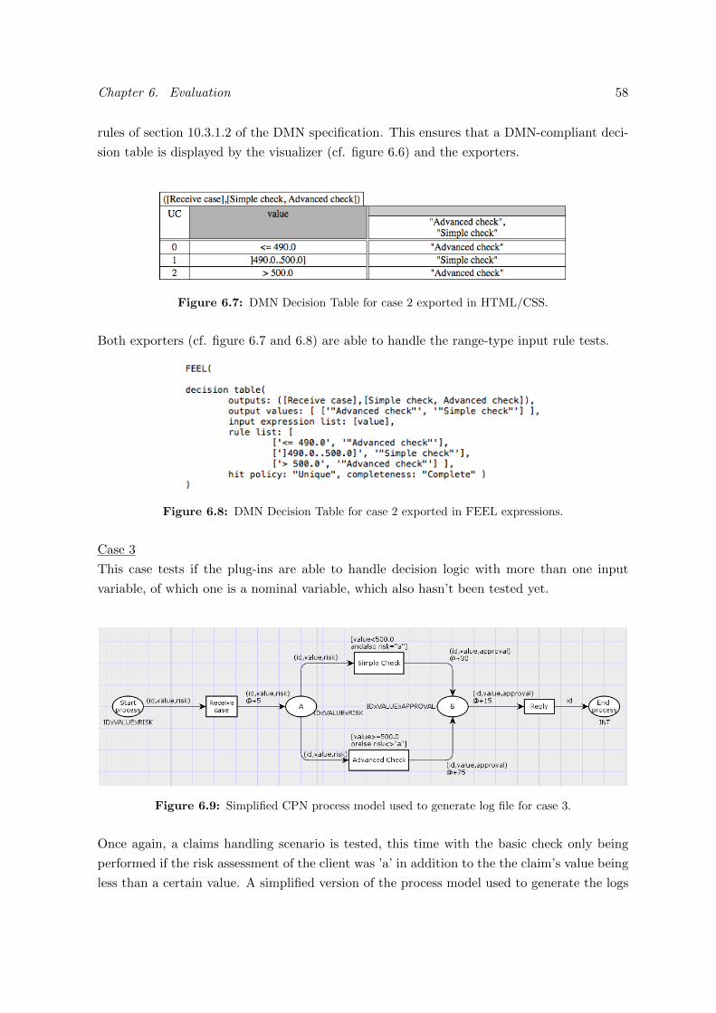
Chapter 6. Evaluation 58
rules of section 10.3.1.2 of the DMN specification. This ensures that a DMN-compliant deci-
sion table is displayed by the visualizer (cf. figure 6.6) and the exporters.
Figure 6.7: DMN Decision Table for case 2 exported in HTML/CSS.
Both exporters (cf. figure 6.7 and 6.8) are able to handle the range-type input rule tests.
Figure 6.8: DMN Decision Table for case 2 exported in FEEL expressions.
Case 3
This case tests if the plug-ins are able to handle decision logic with more than one input
variable, of which one is a nominal variable, which also hasn’t been tested yet.
Figure 6.9: Simplified CPN process model used to generate log file for case 3.
Once again, a claims handling scenario is tested, this time with the basic check only being
performed if the risk assessment of the client was ’a’ in addition to the the claim’s value being
less than a certain value. A simplified version of the process model used to generate the logs

Chapter 6. Evaluation 59
can be seen in figure 6.9.
Figure 6.10: DMN Decision Table Visualizer for case 3.
The workflow is applied and it becomes clear that both the fact that there is more than one
input variable and that these include nominal variables are handled well, both during mining
and visualization, be it in ProM (cf. figure 6.10) or in one of the exporters (cf. figure 6.11).
Figure 6.11: The output of the exporters for case 3 (left: HTML, right: FEEL).
Case 4
This case tests if the plug-ins are able to handle decision logic with multiple values of a nomi-
nal variable leading to a particular decision.6 This also tests if the merging of different rows,
as mentioned in section 5.2, is performed correctly. Once more, the claims handling process is
used, this time with only the risk assessment determining the routing. The simplified process
model utilized to generate the log files used for this case can be found in figure 6.12.
6This is structured in a particular way in the decision tree returned by the Weka algorithm used by the
decision miner and thus needs to be checked separately.

Chapter 6. Evaluation 60
Figure 6.12: Simplified CPN process model used to generate log file for case 4.
The conditions are parsed correctly in all rule entry cells of the DMN table, including the
multi-value not-function. This representation was chosen as it is most easily understood by
the end-user.
Figure 6.13: DMN Decision Table Visualizer for case 4 (top: unsimplified, bottom: simplified).
The resulting decision tables are in line with the underlying decision logic and comply to the
DMN rules. The simplification that is done when the only difference between two rows is the
value of a nominal variable (cf. section 5.2) is clear in this case, as originally three different
rules led to the simple check -activity, one for risk type ’a’, one for risk type ’b’ and one for
risk type ’c’ (upper table in figure 6.13). This was reduced to just one rule (lower table in
the figure).

Chapter 6. Evaluation 61
Figure 6.14: The output of the original DPN Miner for case 4.
Compared to the representation of the decision logic by the unaltered DPN Miner, which can
be seen in figure 6.14, the output of the new package is much more clear and user-friendly,
thus confirming that the main goals of this paper has been achieved. Proper parsing and
presentation of the results of the decision mining has paid off in the shape of a much more
usable overview of the decision logic.
Figure 6.15: The output of the exporters for case 4 (left: HTML, right: FEEL).
Case 5
Case 5 tests if the decision logic for multiple decision points in a single process are extracted
and displayed properly. The scenario is once again the insurance claim handling process, but
now a different reply is sent to the customer depending on the outcome of the (simple or
advanced) check. The latter is a boolean variable, another element that hasn’t been tested
yet. A simplified version of the process model used to generate the logs can be seen in figure
6.16.
Figure 6.16: Simplified CPN process model used to generate log file for case 5.

Chapter 6. Evaluation 62
As can be seen in figure 6.17, both decision points are mined and displayed correctly and
switching between the decision tables is easily done by means of the dropdown menu. The
boolean value that is used in the second decision point is also mined and displayed correctly.
Figure 6.17: DMN Decision Table Visualizer for case 5.
The exporters also have no issues handling multiple decision tables, as can be seen in figure
6.18.
Figure 6.18: The output of the exporters for case 5 (left: HTML, right: FEEL).
Case 6
This final scenario tests how the new package handles decision points with more than two
output options. The claims case is modified to include three different types of checks, de-
pending on the risk classification. The simplified process model used to generate the log files
used for this case can be found in figure 6.19.

Chapter 6. Evaluation 63
Figure 6.19: Simplified CPN process model used to generate log file for case 6.
Judging by figures 6.20 and 6.21, having more than two possible output values doesn’t con-
found the developed package.
Figure 6.20: DMN Decision Table Visualizer for case 6.
Figure 6.21: The output of the exporters for case 6 (left: HTML, right: FEEL).

Chapter 6. Evaluation 64
In all, the package handled all scenario’s with ease7, although they covered a broad range of
possible difficulties falling within the scope defined by section 3.1. The functional requirements
set out in chapter 3 and further specified in section 5.1 were provided to the user and this in
a user-friendly, clear and visually attractive package. All signs indicate that the main goal
of this paper has been achieved, given the improvement in representation of the discovered
decision logic.
7It should be noted that the underlying DPN miner did at times not function as was expected based on
the literature that presented this decision mining plug-in. In one case when fed input containing a simple
three way-split (cf. case 6) based on one ratio scale variable, it would fail to detect a guard for one of the
three options and construct inaccurate guards for the other two options. In another case, a more complex
dataset was provided to the miner. It deduced some guard expressions containing input values, but completely
omitted any mention of which variables these values were linked to. These issues cannot be attributed to the
package that was developed in this paper, as it will still construct a correct decision table, although based on
erroneous decision logic.

Chapter 7
Conclusion and Future Work
Applications of process modeling and mining have shown that they can have numerous advan-
tages for daily practice. Recent advances in decision modeling and mining have made similar
advantages possible, but up to now implementations of decision mining have been lacking in
user-friendly features, such as clear and attractive representation of the discovered decision
logic.
The new DMN notation and in particular the decision tables it specifies, show a way forward
in this regard and have the potential to be to decision modeling what BPMN was for process
modeling.
Up to this point, no implementation of DMN was present in the popular open-source ProM
framework. This paper set out to implement DMN decision tables within the ProM framework
in order to improve the presentation of discovered decision logic and to increase the utility of
ProM and decision mining in general for users outside the scientific community. Given these
goals, special importance was given to good visual presentation, shareability and ease-of-use.1
These objectives were pursued by implementing DMN into ProM based on the DPN Miner.
Based on the cases in chapter 6, it can be concluded that this paper achieved what is set out
to do, as DMN decision tables can now be properly mined and displayed in ProM, they can
be exported, both in very shareable HTML/CSS and in FEEL-expressions, and all of this is
done in a user-friendly and visually pleasing manner. When comparing the developed package
to the output of the original DPN Miner (cf. figure 7.1), there is a clear improvement in the
displaying of discovered decision logic, both in clarity and attractiveness. This is caused by
the implementation of the DMN standard, which was developed for exactly that purpose.
1Many other papers and ProM packages concerning process mining in general have had similar goals of
increasings ProM utility and appeal for business users, such as (Leemans et al. (2014b)) and (Mannhardt et al.
(2015a)).
65

Chapter 7. Conclusion and Future Work 66
Figure 7.1: The presentation of decision logic by the original DPN Miner (left) vs. presentation by
the developed package (right).
During the development of this plug-in, a number of unexpected difficulties were encountered
that ran counter to what literature had insinuated. First of all, development of plug-ins for
ProM was more challenging than the praise for this framework suggested. The options for
writing visualizers are especially inflexible, given the restriction to JComponents. Another
unexpected issue was the performance of the DPN Miner. While the literature that presented
this miner to the public made no mention of issues, in some very simple cases it woefully
underperformed (cf. final footnote of chapter 6).
As in all endeavors worth pursuing, answering the research question posed in this paper raised
new ones and suggested further extensions of the package that was developed.
While the decision tables that are produced comply with the DMN standard and are reaso-
nably clear, they could be simplified further than is currently done (cf. section 5.2) by joining
together Input entry cells in successive rows containing the same value, as described in section
8.2.9 of the DMN specification.
General applicability of the package could be significantly increased by implementing an
algorithm that can verify mutual exclusivity of the discovered rules, so that OR-type gateways
can also be used as input without corrupting the validity or completeness of the decision table.
In the current iteration of the developed package, the hit policy would be wrong in case of
an OR-type gateway, or it would have to be removed, which would cause the decision table
to no longer be DMN-compliant, as the hit policy is obligatory.
Another welcome improvement would be the further integration of the developed package
within process modeling in the broad sense, e.g. by linking the discovered decision logic to
the process model in a visible manner.2 In order to improve the utility for daily practice, this
process model would ideally be a BPMN model. It may be possible to achieve this by means
of a novel combination of existing plug-ins, such as those mentioned in section 2.4. Of course,
the linking of process model and decision logic would preferably be done by means of a DMN
decision requirements graph.
2This extension was explicitly foreseen and kept in mind during the planning of the implementation (cf.
section 5.2).

Chapter 7. Conclusion and Future Work 67
Although not an extension of the work performed in this paper per se, an interesting usage
of the discovered decision logic would be to extend conformance checking beyond the usual
control-flow perspective. Some preliminary work on this subject has already been performed,
e.g. by Mannhardt et al. (2015b).
While this master’s thesis had to overcome quite some hurdles (the visual part of the ProM
framework springs to mind), these challenges were welcome and provided substantial learning-
opportunities, e.g. five different languages were used during this project (Latex, Standard
ML, Java, HTML and CSS). In all, this master’s thesis accomplished the goals it set out
to achieve and advanced the ProM framework in a meaningful way, by allowing users with a
non-scientific background to easily and efficiently go from log files to clear and understandable
decision logic in the form of DMN-compliant decision tables.

Chapter 7. Conclusion and Future Work 68
Bibliography
J. C. M. Baeten & W. P. Weijland (1990). Process Algebra. Cambridge University Press.
E. Bazhenova & M. Weske (2015). Deriving Decision Models from Process Models by Enhan-
ced Decision Mining. In DeMiMoP15 BPM ’15.
A. Bolt, M. de Leoni & W. M. P. van der Aalst (2015). Scientific workflows for process mining:
building blocks, scenarios, and implementation. International Journal on Software Tools
for Technology Transfer.
S. Catalkaya, D. Knuplesch, C. Chiao & M. Reichert (2014). Business Process Management
Workshops: BPM 2013 International Workshops, chapter Enriching Business Process Mo-
dels with Decision Rules, pp. 198–211. Springer International Publishing, Cham.
CODASYL (1982). A Modern Appraisal of Decision Tables, Report of The Decision Table
Task Group. Technical report, New York.
M. de Leoni, M. Dumas & L. Garcıa-Banuelos (2013). Discovering branching conditions from
business process execution logs. In 16th International Conference, FASE 2013, volume 7793
LNCS, pp. 114–129. Springer, Eindhoven.
M. de Leoni & W. M. P. van der Aalst (2013). Data-Aware Process Mining: Discovering De-
cisions in Processes Using Alignments. In Proceedings of the 28th Annual ACM Symposium
on Applied Computing - SAC ’13, p. 1454.
M. de Leoni, W. M. P. van der Aalst & M. Dees (2014). A General Framework for Correlating
Business Process Characteristics. In the 11th Business Process Management (BPM ’14),
pp. 250–266. Springer International Publishing, Eindhoven.
M. de Leoni, W. M. P. van der Aalst & M. Dees (2016). A general process mining framework
for correlating, predicting and clustering dynamic behavior based on event logs. Information
Systems, 56(C):235–257.
A. K. A. de Medeiros, B. F. van Dongen, W. M. P. van der Aalst & A. J. M. M. Weijters
(2005). Ubiquitous Mobile Information and Collaboration Systems: Second CAiSE Work-
69

Bibliography 70
shop, UMICS 2004, Revised Selected Papers, chapter Process Mining for Ubiquitous Mobile
Systems: An Overview and a Concrete Algorithm, pp. 151–165. Springer Berlin Heidelberg.
A. K. A. de Medeiros, A. J. M. M. Weijters & W. M. P. van der Aalst (2007). Genetic process
mining: An experimental evaluation. Data Mining and Knowledge Discovery, 14(2):245–
304.
J. De Weerdt, S. K. L. M. Vanden Broucke & F. Caron (2015). Bidimensional process discovery
for mining BPMN models. In Lecture Notes in Business Information Processing, volume
202, pp. 529–540.
T. Debevoise & J. Taylor (2014). The MicroGuide to Process and Decision Modeling in BPM-
N/DMN: Building More Effective Processes by Integrating Process Modeling with Decision
Modeling. CreateSpace Independent Publishing Platform.
M. Dumas, W. M. P. van der Aalst & A. H. M. ter Hofstede (2005). Process Modeling using
Event-Driven Process Chains. In A.-W. Scheer, O. Thomas & O. Adam, editors, Process-
Aware Information Systems: Bridging People and Software through Process Technology.
Wiley.
A. E. Eiben & J. E. Smith (2003). Introduction to Evolutionary Computing, chapter Genetic
Algorithms, pp. 37–69. Springer Berlin Heidelberg.
U. Fayyad, G. Piatetsky-Shapiro & P. Smyth (1996). From data mining to knowledge discovery
in databases. AI magazine, 17(3):37–54.
D. Grigori, F. Casati, M. Castellanos, U. Dayal, M. Sayal & M.-C. Shan (2004). Business
process intelligence. Comput. Ind., 53(3):321–343.
R. Grossman, S. Bailey, A. Ramu, B. Malhi, P. Hallstrom, I. Pulleyn & X. Qin (1999).
The management and mining of multiple predictive models using the predictive modeling
markup language. Information and Software Technology, 41(9):589–595.
C. W. Gunther & W. M. P. van der Aalst (2007). Fuzzy mining: Adaptive process simplifi-
cation based on multi-perspective metrics. Business Process Management - Lecture Notes
in Computer Science, 4714:328–343.
C. W. Gunther & E. Verbeek (2014). XES standard definition. Technical report.
A. R. Hevner, S. T. March, J. Park & S. Ram (2004). Design Science in Information Systems
Research. MIS Quarterly, 28(1):75–105.
W. Jareevongpiboon & P. Janecek (2013). Ontological approach to enhance results of business
process mining and analysis. Business Process Management Journal, 19(3):459–476.

Bibliography 71
P. Johannesson & E. Perjons (2014). An Introduction To Design Science. Springer Interna-
tional Publishing.
A. A. Kalenkova, M. de Leoni & W. M. P. van der Aalst (2014). Discovering, analyzing and
enhancing BPMN models using ProM. In CEUR Workshop ’14, volume 1295, pp. 36–40.
G. T. Lakshmanan, D. Shamsi, Y. N. Doganata, M. Unuvar & R. Khalaf (2013). A markov
prediction model for data-driven semi-structured business processes. Knowledge and Infor-
mation Systems, 42(1):97–126.
S. J. J. Leemans, D. Fahland & W. M. P. van der Aalst (2014a). Discovering block-structured
process models from event logs containing infrequent behaviour. Lecture Notes in Business
Information Processing, 171 LNBIP:66–78.
S. J. J. Leemans, D. Fahland & W. M. P. Van Der Aalst (2014b). Process and deviation
exploration with inductive visual miner. In CEUR Workshop ’14, volume 1295, pp. 46–50.
N. Lohmann, E. Verbeek & R. Dijkman (2009). Transactions on petri nets and other models
of concurrency ii. chapter Petri Net Transformations for Business Processes – A Survey,
pp. 46–63. Springer-Verlag, Berlin, Heidelberg.
L. T. Ly, S. Rinderle, P. Dadam & M. Reichert (2006). Business Process Management Work-
shops: BPM 2005 International Workshops. Revised Selected Papers, chapter Mining Staff
Assignment Rules from Event-Based Data, pp. 177–190. Springer Berlin Heidelberg.
F. M. Maggi, A. J. Mooij & van der Aalst W M P (2011). User-guided discovery of declarative
process models. In 2011 IEEE Symposium on Computational Intelligence and Data Mining
(CIDM), pp. 192–199.
F. Mannhardt, M. de Leoni & H. A. Reijers (2015a). The multi-perspective process explorer.
In CEUR Workshop ’15, pp. 130–134.
F. Mannhardt, M. de Leoni, H. A. Reijers & W. M. P. van der Aalst (2015b). Balanced
multi-perspective checking of process conformance. Computing, 98(4):407–437.
F. Mannhardt, M. de Leoni, H. A. Reijers & W. M. P. van der Aalst (2016). Decision Mining
Revisited - Discovering Overlapping Rules. In 28th International Conference on Advanced
Information Systems Engineering (CAiSE 2016).
S. Mertens, F. Gailly & G. Poels (2015). Enhancing declarative process models with dmn
decision logic. In K. Gaaloul, S. Nurcan, R. Schmidt, S. Guerreiro & Q. Ma, editors, Lecture
Notes in Business Information Processing, volume 214, pp. 151–165. Springer International
Publishing.
T. M. Mitchell (1997). Machine Learning. McGraw-Hill, Inc., New York, NY, USA.

Bibliography 72
C. Mues, B. Baesens, R. Setiono & J. Vanthienen (2005). From Knowledge Discovery to
Implementation: A Business Intelligence Approach Using Neural Network Rule Extraction
and Decision Tables. In Third Biennial Conference, WM 2005, pp. 483–495.
Object Management Group (OMG) (2009). Production Rule Representation (PRR). URL
http://www.omg.org/spec/PRR/1.0/.
Object Management Group (OMG) (2014). Business Process Model and Notation (BPMN)
Version 2.0.2. URL http://www.omg.org/spec/BPMN/.
Object Management Group (OMG) (2015). Decision Model and Notation (DMN) Version
1.0. URL http://www.omg.org/spec/DMN/.
K. Peffers, T. Tuunanen, M. Rothenberger & S. Chatterjee (2007). A design science re-
search methodology for information systems research. Journal of Management Information
Systems, 24(3):45–77.
M. Pesic, H. Schonenberg & W. M. P. van der Aalst (2007). DECLARE: Full support for
loosely-structured processes. In IEEE International Enterprise Distributed Object Compu-
ting Workshop, EDOC, pp. 287–298.
C. A. Petri (1966). Communication with automata. Ph.D. thesis, Universitat Hamburg.
M. Polato, A. Sperduti, A. Burattin & M. de Leoni (2014). Data-aware remaining time
prediction of business process instances. In 2014 International Joint Conference on Neural
Networks (IJCNN), pp. 816–823.
J. R. Quinlan (1993). C4.5: Programs for Machine Learning. Morgan Kaufmann Publishers
Inc., San Francisco, CA, USA.
I. Raedts, M. Petkovic, Y. Y. S. Usenko, J. M. E. M. van der Werf, J. F. Groote & L. J.
Somers (2007). Transformation of BPMN Models for Behaviour Analysis. In Verification
and Validation of Enterprise Information Systems 2007, pp. 126–137.
A. Rozinat, R. S. Mans & W. M. P. van der Aalst (2006). Mining CPN models: Discovering
process models with data from event logs. Proceedings of the Seventh Workshop on the
Practical Use of Coloured Petri Nets and CPN Tools (CPN 2006), pp. 57–76.
A. Rozinat & W. M. P. van der Aalst (2006a). Decision mining in business processes. BPM
Center Report BPM-06-10.
A. Rozinat & W. M. P. van der Aalst (2006b). Decision mining in prom. In Proceedings of
the 4th International Conference on Business Process Management, BPM’06, pp. 420–425.
Springer-Verlag, Berlin, Heidelberg.

Bibliography 73
B. Silver (2016). DMN Method and Style: The Practitioner’s Guide to Decision Modeling
with Business Rules. Cody-Cassidy Press.
M. Song & W. M. P. van der Aalst (2008). Towards comprehensive support for organizational
mining. Decision Support Systems, 46(1):300–317.
R. A. Sutrisnowati, H. Bae, J. Park & B. H. Ha (2013). Learning Bayesian network from
event logs using mutual information test. In IEEE 6th International Conference on Service-
Oriented Computing and Applications, SOCA 2013, 1, pp. 356–360.
J. Taylor, A. Fish, J. Vanthienen & P. Vincent (2013). Emerging Standards in Decision
Modeling: an Introduction to Decision Model & Notation. In L. Fischer, editor, iBPMS:
Intelligent BPM Systems: Intelligent BPM Systems: Impact and Opportunity, pp. 133–146.
Future Strategies Inc.
W. M. P. van der Aalst (1999). Formalization and verification of event-driven process chains.
Information and Software Technology, 41(10):639–650.
W. M. P. van der Aalst (2011). Process Mining: Discovery, Conformance and Enhancement
of Business Processes. Springer Berlin Heidelberg.
W. M. P. van der Aalst, A. Adriansyah & B. Van Dongen (2011). Causal nets: A mode-
ling language tailored towards process discovery. In Proceedings of the 22Nd International
Conference on Concurrency Theory, CONCUR’11, pp. 28–42. Springer-Verlag, Berlin, Hei-
delberg.
W. M. P. van der Aalst, A. Andriansyah, A. K. A. de Medeiros, F. Arcieri, T. Baier, T. Blickle,
J. C. Bose, P. van den Brand, R. Brandtjen & J. C. a. M. Buijs (2012). Process mining
manifesto. BPM 2011 Workshops Proceedings, pp. 169–194.
W. M. P. van der Aalst, B. F. Dongen, C. W. Gunther, R. S. Mans, A. K. A. de Medeiros,
A. Rozinat, V. Rubin, M. Song, H. M. W. Verbeek & A. J. M. M. Weijters (2007). Petri
Nets and Other Models of Concurrency – ICATPN 2007. Proceedings, chapter ProM 4.0:
Comprehensive Support for Real Process Analysis, pp. 484–494. Springer Berlin Heidelberg.
W. M. P. van der Aalst & A. H. M. ter Hofstede (2005). Yawl: Yet another workflow language.
Information Systems, 30(4):245–275.
W. M. P. van der Aalst, B. F. Van Dongen, J. Herbst, L. Maruster, G. Schimm & A. J.
M. M. Weijters (2003). Workflow mining: A survey of issues and approaches. Data and
Knowledge Engineering, 47(2):237–267.
W. M. P. van der Aalst, A. J. M. M. Weijters & L. Maruster (2004). Workflow Mining:
Discovering Process Models from Event Logs. IEEE Transactions on Knowledge and Data
Engineering, 16(9):549–593.

Bibliography 74
B. F. van Dongen, A. K. A. de Medeiros, H. M. W. Verbeek, A. J. M. M. Weijters & W. M. P.
van der Aalst (2005). The prom framework: A new era in process mining tool support.
In Proceedings of the 26th International Conference on Applications and Theory of Petri
Nets, ICATPN’05, pp. 444–454. Springer-Verlag, Berlin, Heidelberg.
B. F. van Dongen, A. K. A. de Medeiros & L. Wen (2009). Process Mining: Overview and
Outlook of Petri Net Discovery Algorithms. In K. Jensen & W. M. P. van der Aalst, editors,
Transactions on Petri Nets and Other Models of Concurrency II SE - 13, volume 5460 of
Lecture Notes in Computer Science, pp. 225–242. Springer Berlin Heidelberg.
H. M. W. Verbeek, J. C. A. M. Buijs, B. F. Dongen & W. M. P. Aalst (2011). Information
Systems Evolution: CAiSE Forum 2010, Selected Extended Papers, chapter XES, XESame,
and ProM 6, pp. 60–75. Springer Berlin Heidelberg.
A. J. M. M. Weijters & W. M. P. van der Aalst (2003). Rediscovering Workflow Models from
Event-Based Data using Little Thumb. Integrated ComputerAided Engineering, 10:151–162.
A. J. M. M. Weijters, W. M. P. van der Aalst & A. K. A. de Medeiros (2006). Process Mining
with the HeuristicsMiner Algorithm. Cirp Annals-manufacturing Technology, 166:1–34.
M. Werner & N. Gehrke (2013). Process Mining. WISU - die Zeitschrift fur den Wirtschafts-
studenten 7/13, pp. 934–943.

Appendix A
Definitions
• Activity: A well-defined step in a process. Events in a log files (should) refer to a
particular activity.
• Case: An instance of a process, cf. trace.
• Conformance checking: Comparing traces in an event log, i.e. past instances of a
process, against a process model to see whether they diverge from the behavior defined
in that process model, or vice versa.
• Decision logic: The actual rules governing a decision, meaning that they define which
of the output options of a decision are selected in a particular instance based on the
values of the variables that serve as the input for that decision instance.
• Decision point: A point in a process where decision-making occurs, i.e. one or more
alternatives need to be chosen from an array of choices. In this paper, this concerns
choosing between different alternative routings leading out of a particular point in the
process.
• Gateway: Various constructs that split or join different flows in the process. Examples
from BPMN include the exclusive-split gateway and the AND-split.
• Guards: A boolean expression that must evaluate to true in order for an activity to
execute. In this context, these are the conditions, i.e. the decision rules, that need to
be met in order for a particular transition in a Petri net to fire, which is equivalent to
a certain decision being made.
• Log: A file that lists instances of a process that have occurred, as well as the sequence
of activities they were made up of. These concepts translate to respectively traces and
events in log files (cf. section 2.3). In addition, events and traces can contain attributes.1
1This is a fairly strict definition of a log file. One of the largest difficulties in real-world process mining is
75

Appendix A. Definitions 76
• Process mining: Using data-mining algorithms to extract knowledge concerning a pro-
cess based on event log files, i.e. information on past executions of the process. It is an
automated method of process analysis.
• Trace: An instance of a process. A sequence of events (and their attributes, as well as
trace attributes) representing one execution of a process from start to end (de Leoni
et al. (2013)). Also called a case.2
gathering the required information, meaning that one usually doesn’t start out with information that conforms
to this definition.2Some ambiguity on the interpretation of this term is present in literature. E.g. some authors interpret it
as being a particular beginning-to-end-path through the process (meaning that multiple process instances can
have the same trace).

Generating XES Log Files Including Data UsingCPN Tools & XES Logging Formulas
Samuel Peeters1
Faculty of Economics and Business Administration, Ghent University,Tweekerkenstraat 2 9000, Ghent, Belgium
1 Introduction
Using log files generated from a known process model, in this case in the formof a (colored) petri net, has numerous uses in the scientific study of process anddecision mining as they form a perfect dataset with no discrepancies or noise.While some straightforward approaches exist to achieve this (see [2] for anoverview), none of these options were created with the study of decision miningin mind, leading to log files that contain information on control flow, but littleto no additional data hinting at data flow in the process.This document and its accompanying set of functions for CPN Tools1 seek toaddress this issue. They allow the user to generate XES log files including dataelements in the form of (event or trace) attributes in conjunction with CPNTools.2 Using CPN Tools does have a slight learning curve and assumes priorknowledge on (colored) petri nets, but for the stated purpose it is one of themost straightforward approaches.The log functions that are the subject of this document are XES-variants of theones introduced in [1].The following section of this document deals with setting up the functions foryour model and the second section will explaing the different functions and howto add them to your models. Basic knowledge on petri nets and the basic CPNTools-commands will be assumed.
2 Setup
The following sections are partly derived from [1].In order for the functions to work, four declarations need to be added:
1. A value PATH for the path for the logs, e.g.
1 http://cpntools.org/2 Though generating XES-compliant log files in CPN Tools was al-
ready possible using different functions (provided at http://www-inf.it-sudparis.eu/SIMBAD/tools/LogRec/), adding other attributes than the eventnames was not included in the functionality.
Appendix B
Generating Log Files

2
val PATH = "./logs/";
2. A value LOGNAME for the name of the log, e.g.
val LOGNAME = "Example 1";
3. A value FILE_EXTENSION, e.g.
val FILE_EXTENSION = ".XES";
4. An import command for the XES logging formulas, e.g.
use "XESLogging.sml;"
3 Calling the Formulas
Now that the formulas have been set up, the functions to construct the log canbe called. This is done by configuring transactions with code segments callingthe functions. In essence, the model in CPN Tools can be divided into a partwith nodes that pertain only to the generation of log files and a part ’actual’process model (although this part also includes the functions for logging theevents).
Fig. 1. Adding the necessary declarations.
3.1 Creating a New Log
First the log needs to be created by calling the createLog() function.3 Thisfunction will by default add references to the Concept, Time and OrganizationalXES-extensions. A classifier named ’Activity’for the attribute ’concept:name’will also be included. This necessitates the declaration of a global attribute onthe event level for ’concept:name’, which is thus also added.
3 The figures are based on the Example 1 CPN-file, which is bundled with the func-tions.

3
Fig. 2. Transition creating a new log.
3.2 Adding a Trace
The log contains a number of traces (this number can be modeled by creating aloop in the petri net that will perform as many times as the desired amount oftraces). These need to be opened in the log file before the start of the ’actual’process model. This is done by calling the openTrace() function.4 In the case offigure 3, the transaction that does this also binds a random value from a normaldistribution5 to the variable ’value’, which represents the value of an insuranceclaim.
Fig. 3. Transition opening a new trace.
4 These functions are placed under the ’action’ section of the code segment. Any inputpassed as parameters in the functions and coming from the petri net token needsto be mentioned in the input section of the code segment. In case multiple formulasneed to be called by the same transaction, the workaround shown in figure 4 can beapplied.
5 For other distributions, see http://cpntools.org/documentation/tasks/performance/random/start.

4
3.3 Adding Trace Attributes
Next the trace-level attributes are written to the log. There are different func-tions depending on what type of variable you want to log.
– addTraceName(Integer): This function is a shortcut for adding attributesof the type ’concept:name’. It takes an integer as input as it was made toconvert the trace id of the petri net token to the trace name in the XES log.E.g.
addTraceName(id)
– addFloatTraceAttribute(String,Real): Takes a String for the key of the at-tribute and a Real for the value and adds a trace attribute with those pa-rameters to the current trace. E.g. writing the value of the insurance claimto the ’value’ trace attribute of the float type:
addFloatTraceAttribute("value",value)
– addIntTraceAttribute(String,Real): Takes a String for the key of the at-tribute and an Integer for the value and adds a trace attribute with thoseparameters to the current trace.
– addStringTraceAttribute(String,Real): Takes a String for the key of the at-tribute and a Real for the value and adds a trace attribute with those pa-rameters to the current trace.
– addBoolTraceAttribute(String,Real): Takes a String for the key of the at-tribute and a Real for the value and adds a trace attribute with those pa-rameters to the current trace.
Fig. 4. Transition that adds the trace’s name and the value of the insurance claim inthis particular trace.
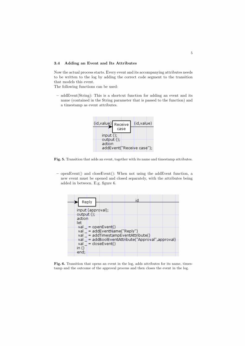
5
3.4 Adding an Event and Its Attributes
Now the actual process starts. Every event and its accompanying attributes needsto be written to the log by adding the correct code segment to the transitionthat models this event.The following functions can be used:
– addEvent(String): This is a shortcut function for adding an event and itsname (contained in the String parameter that is passed to the function) anda timestamp as event attributes.
Fig. 5. Transition that adds an event, together with its name and timestamp attributes.
– openEvent() and closeEvent(): When not using the addEvent function, anew event must be opened and closed separately, with the attributes beingadded in between. E.g. figure 6.
Fig. 6. Transition that opens an event in the log, adds attributes for its name, times-tamp and the outcome of the approval process and then closes the event in the log.

6
– addEventName(String): This function is a shortcut for adding attributesof the type ’concept:name’. It takes a string as input for the value of thisattribute. E.g.
addTraceName("Request approval")
– addTimestampEventAttribute(): This function is a shortcut for adding at-tributes of the type ’time:timestamp’ to an event.
– addBoolEventAttribute(String,Real): Takes a String for the key of the at-tribute and a Real for the value and adds an event attribute with thoseparameters to the current event. E.g.
addBoolEventAttribute("approval",approval)
– addFloatEventAttribute(String,Real): Takes a String for the key of the at-tribute and a Real for the value and adds an event attribute with thoseparameters to the current event.
– addIntEventAttribute(String,Real): Takes a String for the key of the at-tribute and an Integer for the value and adds an event attribute with thoseparameters to the current event.
– addStringEventAttribute(String,Real): Takes a String for the key of the at-tribute and a Real for the value and adds an event attribute with thoseparameters to the current event.
3.5 Closing a Trace
Once all events for a particular trace have been added, the trace needs to beclosed by calling the closeTrace() function. E.g. figure 7.
Fig. 7. Transition that closes the current trace in the log.
3.6 Closing a Log
After all traces have been added, the log needs to be closed by calling thecloseLog() function. E.g. figure 8

7
Fig. 8. Transition that closes the log file.
References
1. de Medeiros, A. K. A., & Gnther, C. W. (2005). Process Mining: Using CPN Toolsto Create Test Logs for Mining Algorithms. Proceedings of the Sixth Workshopand Tutorial on Practical Use of Coloured Petri Nets and the CPN Tools, 177190.http://doi.org/10.1.1.60.460
2. vanden Broucke, S. K. L. M., Vanthienen, J., & Baesens, B. (n.d.). StraightforwardPetri net-based event log generation in ProM.


![New Features in DMN 1 - RuleML2017.ruleml-rr.org/wp-content/uploads/2017/06/DC2017...Agreed for DMN 1.2 • New features Annotation columns in decision tables [12-124] • Removed](https://static.fdocuments.in/doc/165x107/60082e0ef625c246b653149f/new-features-in-dmn-1-agreed-for-dmn-12-a-new-features-annotation-columns.jpg)


![Generating Decision-Aware Models & Logs: Towards an ... · gaining momentum due to the introduction of the Decision Model and Notation (DMN) standard [1]. Decision mining focuses](https://static.fdocuments.in/doc/165x107/5ec7e2da545247384a4f3069/generating-decision-aware-models-logs-towards-an-gaining-momentum-due.jpg)