Keller #38

DECISION ANALYSIS WITH

GEOGRAPHICALLY VARYING OUTCOMES: PREFERENCE MODELS AND ILLUSTRATIVE APPLICATIONS

JAY SIMON Defense Resources Management Institute, Naval Postgraduate School, Monterey, CA 93943, jrsimon@nps.edu

CRAIG W. KIRKWOOD W. P. Carey School of Business, Arizona State University, Tempe, AZ 85287-4706, craig.kirkwood@asu.edu

L. ROBIN KELLER The Paul Merage School of Business, University of California, Irvine, CA 92697-3125, lrkeller@uci.edu

This paper presents decision analysis methodology for decisions based on data from geographic

information systems. The consequences of a decision alternative are modeled as distributions of

outcomes across a geographic region. We discuss conditions which may conform with the decision

maker’s preferences over a specified set of alternatives; then we present specific forms for value or utility

functions that are implied by these conditions. Decisions in which there is certainty about the

consequences resulting from each alternative are considered first; then probabilistic uncertainty about the

consequences is included as an extension. The methodology is applied to two hypothetical urban

planning decisions involving water use and temperature reduction in regional urban development, and fire

coverage across a city. These examples illustrate the applicability of the approach and the insights that

can be gained from using it.

Subject classifications: decision analysis; geographic information systems; multiattribute utility;

multiattribute value; additive independence; preferential independence; homogeneity.

Area of review: Decision Analysis. History:

Forthcoming, Operations Research as of 8-14-13 _____________________________________________________________________________________________

2

1. Introduction

This paper discusses decision analysis methodology that explicitly accounts for outcomes distributed

across a geographic region. As an example, consider a situation where regional planners are considering

alternative development plans that could have varying environmental or socioeconomic impacts across a

region. To support their policy and planning decisions, planners can consider multiple geographic maps

showing current and potential future levels of environmental pollutants, urban development, water

availability, air temperature, etc., that could vary across the region in different ways depending on which

alternative is implemented.

The outcomes of selecting different alternatives in decisions supported by geographic information

can be described in terms of one or more attributes (e.g., maximum outdoor air temperature in July)

whose levels (e.g., 38° Celsius) are known, or can be estimated with some uncertainty over a region. The

levels of these attributes may depend on both the alternative that is selected and the geographic location

within the region of interest.

Park Example: The decision of whether or not to develop a proposed large new landscaped park

could affect the maximum July outdoor air temperature in the region near the proposed park. The

maximum July temperature at any specific location might differ depending on the direction and distance

of that location from the proposed park. We will return to this park example throughout the paper to

illustrate analysis concepts that we present.

For this paper, we define a consequence as a function that assigns levels to each attribute for an

alternative and whose domain is the geographic region of interest. (In the geographic information

systems (GIS) context, the assignment of attribute levels could be done in an automated manner by the

GIS software.)

Thus, to judge the relative desirability of the alternatives, the decision maker must combine the

geographically-varying attribute levels for each alternative. The question we address is: When each

alternative can be represented by one or more maps showing attribute levels over a geographic region that

3

would result from selecting that alternative, how can a decision maker determine the relative desirability

of each alternative?

This paper discusses preference models for a decision analysis approach to such decisions. We

use the term preference model to designate i) conditions on decision maker preferences for the potential

consequences from a specified set of alternatives as described by the attributes and ii) the possible forms

of functions that will obey those conditions which can be used to evaluate alternatives. Such functions are

called preference functions. Decisions in which there is certainty about the consequences resulting from

each alternative are considered first, then decisions with probabilistic uncertainty about the consequences

are considered. (The resulting preference functions are called value functions for decisions under certainty

or utility functions for decisions under uncertainty.) We describe procedures to assess value functions of

the type presented in this paper and illustrate the use of these preference models with hypothetical

applications in two potential problem domains: Water use and temperature reduction tradeoffs in regional

urban development and fire coverage across a city.

2. Applications of Geographic Information Systems

The use of maps generated by computer-based geographic information systems (GIS) has become

widespread due to increasing computer capabilities and decreasing costs (Obermeyer and Pinto 2007),

and such analysis is the basis for a large stream of literature. GIS analyses have been applied, for

example, to irrigation and water resource management (Knox and Weatherfield, 1999), wildlife habitat

selection in Alaska (Pendleton et al., 1998), and deforestation (Kohlin and Parks, 2001). Arbia (1993)

provides a detailed overview of GIS, including consideration of sampling and modeling errors but not

analysis of uncertainty over consequences or consideration of preferences.

The lack of explicit decision analysis methods is a limitation in most previous GIS work that

hinders its use for comparing alternatives or designing new alternatives which would have equivalent or

higher value. There has been limited application of preference models to address decisions using GIS

data. Instead, most GIS research has focused on statistical approaches for analyzing the data (Bond and

4

Devine, 1991), or improved methods to display data to stakeholders (Koller et al., 1995; Slocum et al.,

2001). Worrall and Bond (1997) explore some of the reasons GIS tools have yielded fewer benefits than

expected in the public sector; one of these reasons is a lack of effective decision support systems. As we

will demonstrate, adding a decision analysis component to the analysis of geographic information can

increase the power of GIS tools to support policy decision making.

A small subset of the GIS literature addresses decision making. De Silva and Eglese (2000)

discuss the development of a decision support system which connects GIS data to a simulation model for

evacuations. Malczewski (1999) and Jankowski (1995, 2006) provide more detailed analysis of multi-

criteria decisions using GIS data. Chan (2005) examines the use of multi-criteria decision making in a

broad context of spatial applications. However, the decisions considered by these authors do not directly

involve preferences over consequences. Keisler and Sundell (1997) use a somewhat different approach

for a park planning problem, by modeling multiattribute utility over aggregated attribute levels within a

geographic region. These aggregated levels are affected by the decision maker’s choice of where the

boundary of the region is drawn. In contrast, we consider preference models that directly address

attributes whose levels may vary across a geographic region.

3. Preference Models for Spatial Decisions Under Certainty

This section presents four preference models for geographically-oriented decision making where potential

consequences of alternatives are known with certainty. Two of the preference models are discrete,

meaning that there are a finite number of subregions and the attribute levels do not vary within any

specified subregion (but may be different in different subregions), and two are non-discrete, meaning that

the region cannot be divided into subregions within which the attribute levels do not vary. For both

discrete and non-discrete situations, we present both a single-attribute and a multi-attribute preference

model, so there are a total of four different models.

Keeney and Raiffa (1976) present and demonstrate the use of preference models over a discrete

number of attributes. Such models are now widely used to determine the relative desirability of multiple-

5

attribute alternatives, where each alternative takes on a specific level on each of the multiple attributes

1 2, , , nZ Z Z , and zi designates a specific level of Zi. (Keeney and Raiffa denote the attributes and levels

as Xi and xi, respectively, but we use Zi and zi to avoid confusion with the use of x as a spatial dimension

later in this paper.) For example, a decision related to locating a new store branch might have attributes

such as the distance from the closest competitor, distance from the warehouse, and population size within

a five-mile radius. For decisions with no uncertainty, preferences over the consequences of these

alternatives are represented by a multiattribute value function 1 2( , , )nV z z z . See Debreu (1954, 1964),

Fishburn (1970), and Krantz et al. (1971) for expositions of the relevant preference theory. Keeney and

Raiffa (1976), Keeney (1992), and Kirkwood (1997) have more elementary presentations. See Keefer et

al. (2004) for a review of decision analysis applications.

In the discrete preference models in this paper, the region is partitioned into m discrete

subregions, labeled 1, ..., m, such that the level of an attribute does not vary within any specified

subregion. In the non-discrete preference models in this paper, the level of an attribute depends on the

geographic coordinates x and y that designate a location within the region. In the single-attribute models,

the consequences are described by functions that assign a single number (the attribute level) to each

subregion (for the discrete case) or location (for the non-discrete case), and in the multi-attribute models,

the consequences are described by functions that assign a vector of attribute levels to each subregion (for

the discrete case) or location (for the non-discrete case). In both the discrete and non-discrete cases, the

level or levels that are assigned will depend on the alternative that is selected.

3.1. Spatial Decisions with a Single Attribute.

3.1.1. Discrete Subregions Case. We first consider the case of one attribute with discrete subregions,

and we assume there is a single attribute Z whose domain is a closed interval I, where z designates a

specific level of Z . The region is partitioned into m subregions, and the level of Z does not vary within

any specified subregion. We designate the level of Z in subregion i by iz , thus a consequence can be

expressed as a vector of levels across all subregions 1, , mz zz such that iz I for 1, , i m .

6

A relatively simple value function to represent preferences for the possible consequences of

selecting different alternatives exists if the preferences meet six conditions. Four of these conditions

(completeness, transitivity, continuity, and dependence on each subregion) will always be met in practical

decision making situations. The other two conditions, pairwise spatial preferential independence and

homogeneity, are more restrictive but will be reasonable for many decisions. Preferential independence is

presented in more detail in Appendix A. All six conditions are specified explicitly in Appendix B.

Described informally, pairwise spatial preferential independence requires that value tradeoffs

between the attribute levels in any pair of subregions do not depend on the attribute levels in the other

subregions so long as the levels in the other subregions are common. That is, if a decision is between two

alternatives that only differ on Z in two subregions, then the preferred alternative will not change if the

alternatives are modified by changing the level of Z in the other subregions so long as those levels in the

other subregions are the same for the two alternatives. As an example, suppose for the park decision

discussed above that two alternatives will result in the same temperature outcomes for all except two

specified subregions, and one alternative will give temperatures of 35° and 45° Celsius in those two

subregions while the other alternative will give temperatures of 38° and 42° in the two subregions.

Suppose the second alternative is preferred to the first. If pairwise spatial preferential independence

holds, then this will continue to be true even if the temperatures in the other subregions change, so long as

the temperature in each of the other subregions remains the same for the two alternatives. This condition

implies that this property will hold for any two subregions. (Situations in which it can fail to hold

generally involve decision maker preferences that consider complex interactions between subregions.)

The homogeneity condition requires, stated informally, that relative preferences for different

levels of Z within any subregion will be the same for every subregion. More specifically, the

homogeneity condition holds if the same tradeoffs midvalue is found in every subregion. The detailed

definition of a tradeoffs midvalue is in Appendix B, and the concept can be illustrated with the park

decision for a desert area example: Suppose a decision maker would be willing to give up 2 degrees, from

43° to 45°, in increased maximum temperature in all of the other subregions to decrease the maximum

7

temperature in the specified subregion from 48° to 40°, and similarly would be willing to give up 2

degrees, from 43° to 45°, in increased maximum temperature in all the other subregions to decrease the

maximum temperature in the specified subregion from 40° to 36°. Because the decision maker is willing

to incur the same losses to improve from 48° to 40° as to improve from 40° to 36° in the specified

subregion, 40° is a tradeoffs midvalue for the interval from 36° and 48° in that subregion. The

homogeneity condition holds if 40° is also a tradeoffs midvalue between 36° and 48° in every subregion.

(Situations in which this condition can fail to hold generally involve an attribute for which the decision

maker believes different levels have qualitatively different implications in different subregions.)

When these two conditions, along with the other four specified in Appendix B, hold, then the

following Theorem specifies the form of the value function. The discussion of why this result holds is in

Appendix B.

THEOREM 1. For a region with three or more subregions and a preference relation ~ (“at least as

preferred as”) on the set of consequences 1, , mz z such that iz I for 1, , i m for a closed

interval I , there exists a value function of the form:

1 2

1

( , , , ) ( )m

m i i

i

V z z z a v z

, (1)

if and only if the conditions given in Appendix B for this Theorem hold, where v(zi) is a (common) single

attribute continuous value function over zi, and ai is a positive weight on subregion i.

Thus, when the required conditions hold, it is only necessary to assess one single attribute value function

and a weighting constant for each subregion. This decomposition has intuitive appeal because it separates

the preferences over the attribute levels, which are addressed in v(zi), from the priority or weighting

assigned to each subregion, which is encoded in ai. In some cases subregions will be weighted equally,

and then all ai can be set equal to one so the weights can be eliminated from the equation. For the

8

analogous context of decisions with a stream of outcomes over time, the form of equation (1) has been

previously applied with the ai’s being interpreted as time discounting weights (Harvey, 1986, 1995).

Krantz et al. (1971, pp. 303-305) and Harvey (1986, 1995) show conditions for the existence of a value

function of the form of (1), following up on a question raised about this by Fishburn (1970, p. 93).

The conditions required for (1) may seem restrictive for some decision situations with

geographically varying consequences. However, the resulting value function given by (1) is more general

than most summary metrics typically used in GIS analysis. Those summary metrics are often averages of

the attribute levels, which are special cases of the models we present. For example, to specify conditions

that imply averages can be used in place of the more general formula in (1) requires including a stronger

condition that the tradeoffs midvalue of any interval will be the average of the low and high levels in the

interval (see Appendix B for details). For the park example discussed above, this would mean that the

midvalue between any two temperatures will be the average of the two temperatures. For example, the

midvalue between 5° and 10° will be (5 10) / 2 7.5 °, and similarly the midvalue between 25° and 30°

will be 27.5°, and between 40° and 45° will be 42.5°. In this case, as described in Appendix B,

preferences over the set of consequences can be represented by:

1 2

1

( , , , )m

m i i

i

V z z z a z

(2)

for some set of weights ai. If each 1/ia m , the value function computes the simple (unweighted)

average across subregions. A similar condition can be constructed for the other preference models

presented below, resulting in analogous linear special cases. While this may be reasonable in some

decision situations, (1) allows for more general preference models.

3.1.2. Non-discrete Case. In GIS applications with a large number of subregions, a useful modeling

approach could be to consider the data to vary in a non-discrete manner across the region. For example,

suppose an application addresses land use policy making for an urban area with 100,000 land parcels.

The characteristics of each parcel will vary from the parcel next to it, but not in an extreme manner,

9

except possibly at boundaries between land use categories. In this setting, a non-discrete model could be

easier to analyze than a discrete model with 100,000 subregions. In section 5.2, we provide such an

example.

A non-discrete model can be specified as follows: Assume ~ is a preference relation (“at least as

preferred as”) over the set of consequences, where the consequences are defined in a non-discrete manner

on locations rather than on discrete subregions. With this assumption, a consequence can be expressed as

a function ( , )z x y that determines the level z at each location ( , )x y in the region of interest. Thus,

potential consequences are in the set of ( , )z x y such that ,z x y I for a closed interval I for all

locations ( , )x y within the region. With this formulation, it seems reasonable that an analogous result to

Theorem 1 could be developed to provide a specific form for the value function. In the absence of

discrete subregions, it is reasonable that the sum in (1) would be replaced with an integral over the region.

We provide the following Conjecture for this situation.

CONJECTURE 1. A preference relation ~ on the set of consequences such that ,z x y I for a closed

interval I for locations ,x y within a region of interest A can be represented by a value function of the

form:

( ) ( , ) [ ( , )]A

V z a x y v z x y dxdy (3)

where a and v are bounded and continuous almost everywhere if and only if the conditions given in

Appendix C for this Conjecture hold, where x and y are coordinates within the region, v is a (common)

single attribute continuous value function over z, and ),( yxa is a weight for location (x,y), which is

positive almost everywhere.

This can also be generalized from x and y to any number of indices for the consequences. We

thank an editor for pointing this out and noting that practical examples of this include situations where

time could be a third index, or the spatial index of interest might be one-dimensional, such as locations

10

along a road or a river. In addition, while we interpret ( , )a x y as a weighting function, it could also be

viewed more broadly as a generating function for a transform of [ ( , )]v z x y .

Details of how (3) might be developed from preference conditions analogous to the conditions in

Theorem 1 are in Appendix C, though we do not have a proof of the exact conditions required. Key

requirements are non-discrete analogs of pairwise spatial preferential independence and homogeneity,

plus “reasonable” behavior for preferences as the location varies. Stated informally, reasonable behavior

means there should not be large abrupt changes in characteristics that impact preferences as x and y

vary over small intervals. For example, in the park example, land use should not change back and forth

every few feet across the region. (Discontinuities along continuous curves, such as occur at a park

boundary, do not cause problems.) It is unlikely that such challenges will arise in practical situations

where a non-discrete preference model might be considered.

3.2. Spatial Decisions with Multiple Attributes.

3.2.1. Discrete Subregions Case. Thus far, we have considered only a single attribute defined across a

region. Some decisions will address multiple attributes, one or more of which can vary geographically.

For example, a park planning decision in an arid region might require consideration of both the maximum

July temperature and the groundwater level in different subregions. Incorporating multiple attributes is a

conceptually straightforward extension provided that the appropriate preference conditions hold. We first

consider the situation where there are m subregions, and within each subregion the levels for the attributes

do not vary. Let n designate the number of attributes, and let ijZ designate the jth attribute in the i

th

subregion, where ijz stands for a specific level of that attribute in that subregion, with j

ijz I for all i,

where jI is the closed interval domain of the j

th attribute. We refer to ijZ as an “attribute-subregion

combination”. Let Z designate the set of consequences, where a consequence z Z specifies ijz for

all nm attribute-subregion combinations. As above, let ~ be a preference relation on the set of

consequences.

11

We now present an analogous theorem to Theorem 1 for the case of multiple attributes. The

conditions needed for this theorem to hold are similar to those for Theorem 1, except that pairwise

preferential independence must hold both across subregions and across the multiple attributes.

THEOREM 2. For a preference relation ~ on the set Z of consequences over a region such that

j

ijz I for all subregions i and attributes j, for closed intervals jI , there exists a multiattribute value

function of the form:

1 1

( ) ( )m n

i j j ij

i j

V a b v z

z , (4)

if and only if the conditions given in Appendix D for this Theorem hold, where m ≥ 2, n ≥ 2, ai is a

positive weight for subregion i, bj is a positive weight for the jth attribute, and )( ijj zv is a single attribute

continuous value function over the level of the jth attribute in subregion i. (Note that v only depends on the

attribute index j.)

This result follows from applying results by Gorman (1968) in combination with homogeneity

concepts similar to those studied by Harvey (1986, 1995). A more detailed discussion of this theorem is

included in Appendix D. We present a two-attribute, ten subregion example of the use of (4) for an urban

development decision in section 5.1.

3.2.2. Non-discrete Case. The following Conjecture 2 extends Theorem 2 to the situation where the

(multi-attribute) consequences are functions of locations rather than discrete subregions. Thus, this

conjecture extends Theorem 2 analogously to the way that Conjecture 1 extends Theorem 1. As in

Section 3.1.2, we conjecture that preferences in such a situation which satisfy a set of conditions can be

represented by a value function.

Let ( , )jZ x y designate the jth attribute at location ),( yx , and ( , )jz x y designate the level of

( , )jZ x y . Let Z designate the set of consequences, and let z designate a specified consequence, where

12

1, , , , ,nx y z x y z x y z , and ,j jz x y I for closed intervals jI for all j, for all ,x y

within the region of interest. As previously, let ~ be a preference relation on the set of consequences.

We conjecture the following.

CONJECTURE 2. A preference relation ~ on the set Z of consequences such that ,j jz x y I for all

attributes j and locations ,x y within a region of interest A for closed intervals jI can be represented

by a value function of the form:

1

( ) ( , ) [ ( , )]n

j

j j

jA

V a x y b v z x y dxdy

z (5)

where 1, , , na v v are bounded and continuous almost everywhere if and only if the conditions given in

Appendix E for this Conjecture hold, where x and y are coordinates within the region, jv is a single

attribute continuous value function for the jth attribute, ( , )a x y is a weight for location ),( yx , which is

positive almost everywhere, and bj is a positive weight for the jth attribute.

As with Conjecture 1, we have not been able to prove this result, but it should be clear in practical

decision situations whether this is a reasonable model. Further details are in Appendix E.

4. Value Model Assessment Procedures

This section summarizes approaches for assessing single-attribute value functions, weights, and

preference conditions for (1), (3), (4), and (5). Following the usual convention, we assume without loss of

generality that 1) single-attribute value functions are scaled so the most preferred level of each attribute

that is being considered has a value of one and the least preferred level that is being considered has a

value of zero, and 2) the weights are scaled to sum to one in (1) and (4), or integrate to one in (3) and (5).

4.1. Assessing Single-Attribute Value Functions.

Standard procedures can be used to assess the single-attribute value functions in (1), (3), (4), and (5).

(See, for example, Keeney and Raiffa 1976, Section 3.7.2 or Kirkwood, 1997, p. 240, Step 3.) Often

13

value functions will increase or decrease monotonically over levels of the attribute, such as value

functions for median family incomes or levels of pollution. (If a value function is not monotonic, it can

be possible to redefine the attribute as the distance from an “ideal point” level, in which case the

redefined attribute will be monotonic.) With monotonic preferences, single-attribute value functions can

be assessed using the midvalue splitting approach, using the concept of the tradeoffs midvalue described

in section 3.1.1. For example, suppose a value function is being assessed for profit in subregion i ,

ranging from $0 to $100,000, with higher profits being preferred. The value function is scaled by setting

$0 0v and $100,000 1v . Suppose the tradeoffs midvalue of [$0, $100,000] is determined to be

x = $40,000, i.e. the profit level x such that the decision maker would accept the same decreases in profit

in the other subregions to improve profit in subregion i from $0 to $x or from $x to $100,000. Then it

follows directly from (1) that $40,000 0.5v . The tradeoffs midvalue of [$0, $40,000] or [$40,000,

$100,000] could then be assessed, yielding attribute levels which have single-attribute values of 0.25 and

0.75, respectively, in (1). This procedure could be continued to assess as many specific values as desired.

Alternatively, if the preference conditions hold so that a specific functional form is valid for the single-

attribute value function, then the parameter(s) for the functional form can be determined to specify the

value function. For example, an exponential form for the single-attribute value function is valid if the

relative position of the tradeoffs midvalue within any specified interval depends only on the length of the

interval, and not on its location in the domain of the value function (Kirkwood and Sarin 1980). In this

case, only a single parameter is needed to specify the value function, and that can be determined by

assessing one tradeoffs midvalue. This is illustrated by the examples in Section 5.

4.2. Assessing Weights.

The value tradeoff method (Keeney and Raiffa 1976, Section 3.7.3, Eisenführ et al. 2010, Section 6.4.2)

can be used to determine the subregion weights ai in (1). First, have the decision maker consider m

distinct hypothetical consequences consisting of the most preferred possible level *z of the attribute in a

subregion i, and the least preferred possible level 0z of the attribute in all of the other m – 1 subregions.

14

So, the first hypothetical consequence has the best level in subregion 1, the second has the best level in

subregion 2, etc. Then, have the decision maker determine which of these m consequences is most

preferred, and let *i represent the subregion in which the most preferred level of the attribute is achieved.

Subregion *i will have the highest weight, and can be considered the most important subregion to this

decision maker. For each other subregion *i i , determine the attribute level

iz such that a consequence

consisting of iz in subregion *i and

0z in all other subregions is equally preferred to a consequence

consisting of *z in subregion i and

0z in all other subregions. As stated above, we assume that in (1),

0 0v z and * 1v z . Thus, from the assessed indifference relationship between achieving *z in

subregion i or achieving iz in subregion *i , it follows from direct substitution into (1) that

*

*, 1, ,i iia a v z i m i i . Since the weights are assumed to sum to 1,

1

1m

i

i

a

, and solving the

resulting system of m equations yields the set of weights.

The value tradeoff method above can be adapted to determine the weighting function ( , )a x y for

the non-discrete case represented by (3), but modifications are needed because there are an uncountably

infinite number of weights to be determined. We address this in Section 5.2 for a specific example.

Analogous procedures can be used to determine , 1, ,ia i m , and , 1, ,jb j n , in the

discrete multi-attribute case represented by (4). The form of (4) allows the two sets of weighting

constants to be determined separately, as follows. First determine the subregion weights ia by

considering hypothetical consequences that have the same levels for all attributes except one arbitrary but

specified attribute j . Due to the form of (4), it does not matter which attribute j is used for the

assessment procedure. Assume for these hypothetical consequences that the other attributes are at their

least preferred levels, meaning that their single-attribute values are zero, and then (4) reduces to

1

( ) ( )m

j i j ij

i

v b a v z

z . Since jb is a constant, this equation has the same form as the single-attribute case

15

represented by (1), and thus the same weight assessment procedure presented above for (1) can be applied

to attribute j across the subregions to determine a set of equations * ( ),j i j j ijib a b a v z

*1,2, , ;i m i i , where *i is the most important subregion, and ijz is the level of attribute j in

subregion *i that generates the indifference relationship described above for the single-attribute case.

The jb cancels out of the equations, and combining these equations with 1

1m

i

i

a

gives a set of m

equations that can be solved for the ia just as was done in the single-attribute case. An example of such

an indifference relationship is shown in Table 1, with 3m , 4n , * 1i , and 1j .

Attribute j ( 4n )

Subregion i Consequence 1 Consequence 2

( 3m ) 1 2 3 4 1 2 3 4

*1 i 21z - - - - - - -

2 - - - - *

21z - - -

3 - - - - - - - -

Table 1. A pair of indifferent consequences used in determining a set of subregion weights 1 2 3, ,a a a for

(4). Dashes indicate least-preferred attribute levels, and *

21z represents having the most preferred level of

attribute 1 in subregion 2. This indifference judgment results in the equation 1 2 1 1 1 21( )b a b a v z .

A corresponding procedure can be applied to determine the attribute weights jb by considering

hypothetical consequences that have the same attribute levels in all subregions except one arbitrary but

specified subregion i . As before, it does not matter which subregion is used for the assessment

procedure, and we can assume the attribute levels for the other subregions to be their least preferred

levels, so that equation (4) reduces to 1

( ) ( )n

i j j ij

j

v a b v x

z . In this case, ia is constant, and thus the

equation again has the same form as (1). Applying the same weight assessment procedure to subregion i

across the attributes determines the set of equations * *

*( ), 1,2, , ;i j i ijj ja b a b v z j n j j , where

*j is

16

the most important attribute and ijz is the level of attribute

*j in subregion i that generates the

indifference relationship described above for the single-attribute case. The ia cancels out of the

equations, and combining these equations with 1

1n

j

j

b

gives a set of n equations that can be solved

for the jb . An example of such an indifference relationship for attribute weights is shown in Table 2,

with 3m , 4n , * 1j , and 1i .

Attribute j ( 4n )

Subregion i Consequence 1 Consequence 2

( 3m ) *1 j 2 3 4

*1 j 2 3 4

1 12z - - - - *

12z - -

2 - - - - - - - -

3 - - - - - - - -

Table 2. A pair of indifferent consequences used in determining a set of attribute weights 1 2 3 4, , ,b b b b for

(4). Dashes indicate least-preferred attribute levels, and *

12z represents having the most preferred level of

attribute 2 in subregion 1. This indifference judgment results in the equation 1 2 1 1 1 12( )a b a b v z .

It could be useful to conduct this procedure using more than one attribute to check for consistency

in the responses and to test whether the decision maker’s preferences meet conditions for (4) to be valid.

Similarly it could be useful to assess the ia using more than one subregion.

4.3. Testing Preference Conditions.

The specific conditions that must be checked depend on which single or multiple attribute preference

model, in a discrete subregions case or a non-discrete case, is being applied. As discussed in Section 3,

the key conditions that must be checked are preferential independence and homogeneity. If there are

multiple attributes, then preferential independence must be checked for attributes as well as across

subregions. (In the Appendices, these conditions are (e) and (f) for Theorem 1 and the corresponding

conditions for Theorem 2 and the two Conjectures.)

17

For example, if (1) is to be used for the single attribute and discrete subregions case, then

pairwise spatial preferential independence can be checked by asking the decision maker whether changing

the common level of the attribute in the other subregions would cause a preference reversal for

alternatives that differ only with respect to a pair of subregions. Homogeneity can be checked by asking

the decision maker whether the tradeoffs midvalue for a specified interval is the same for different

subregions. This was discussed for the park example in Section 3.1.1. Analogous checks can be made for

the single attribute non-discrete case.

If the conditions for (1) hold, then the special case of the linear model given by (2) can be used

for the single attribute discrete subregions case if the tradeoffs midvalue for any interval for a given

attribute is equal to the average of the high and low levels of the interval. In the park example, this would

imply, for example, that the tradeoffs midvalue of the interval from 36° to 48° is o(36 48) / 2 42 .

Similar procedures can be used to check the conditions required for the multiple attribute models.

Kirkwood (1997, pp. 239-240, Step 2) discusses testing for preferential independence in further detail.

5. Examples

This section presents two hypothetical examples which apply the preference models discussed above and

shows insights that can be gained from using these models. The first example uses a two-attribute model

with 10 discrete subregions and the second one uses a single attribute non-discrete model. The analysis

for these applications was conducted using Excel Solver, with some use of Visual Basic for Applications.

As discussed in Section 2, the use of these preference models differs from the approaches in previous

applications of GIS data in that decision maker preferences are explicitly specified over spatially-varying

attributes, rather than assessed at an aggregate level, such as the average attribute level over the region.

5.1. Water Use and Temperature Reduction in Regional Urban Development.

Many decisions involving GIS data address multiple attributes. (For example, Keller et al. 2010 found

multiple attributes used by stakeholders in Arizona water resource planning.) The application in this

18

section illustrates the use of Theorem 2 from Section 3.2.1 in such decisions. The data used in this

application come from Gober et al. (2010), who applied a heat flux model to investigate urban heat island

effects in Phoenix, Arizona. Urban development has led to increased temperatures in Phoenix, mostly by

reducing the amount of night cooling that occurs. As a result, there is motivation to increase the quantity

of vegetation, as “green” areas acquire and retain less heat. However, this would also require more water,

as green areas lose more to evaporation than developed urban areas. Thus, night cooling and evaporation

rate are both important considerations when choosing development strategies.

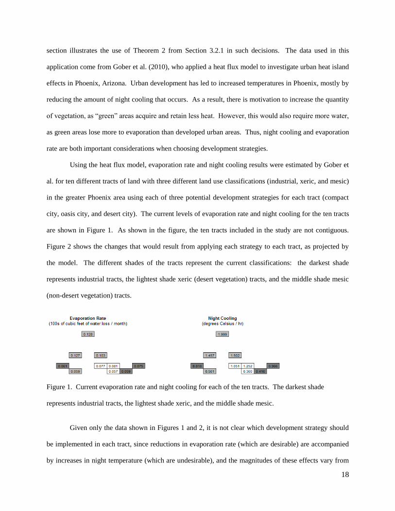
Using the heat flux model, evaporation rate and night cooling results were estimated by Gober et

al. for ten different tracts of land with three different land use classifications (industrial, xeric, and mesic)

in the greater Phoenix area using each of three potential development strategies for each tract (compact

city, oasis city, and desert city). The current levels of evaporation rate and night cooling for the ten tracts

are shown in Figure 1. As shown in the figure, the ten tracts included in the study are not contiguous.

Figure 2 shows the changes that would result from applying each strategy to each tract, as projected by

the model. The different shades of the tracts represent the current classifications: the darkest shade

represents industrial tracts, the lightest shade xeric (desert vegetation) tracts, and the middle shade mesic

(non-desert vegetation) tracts.

Figure 1. Current evaporation rate and night cooling for each of the ten tracts. The darkest shade

represents industrial tracts, the lightest shade xeric, and the middle shade mesic.

Given only the data shown in Figures 1 and 2, it is not clear which development strategy should

be implemented in each tract, since reductions in evaporation rate (which are desirable) are accompanied

by increases in night temperature (which are undesirable), and the magnitudes of these effects vary from

19

tract to tract. Thus, to defensibly choose the optimal development strategy, we should specify a value

function to determine an overall value for different combinations of evaporation rate and night cooling

across the ten tracts. If the conditions for Theorem 2 hold, then to determine a value function we need to

specify single attribute value functions for evaporation rate and night cooling, as well as weights Eb and

Nb for the two attributes and weights , 1, ,10ia i , for each of the ten tracts.

Figure 2. Changes in evaporation rate and night cooling that would result from implementing each of the

three strategies in the ten tracts. The different shades represent the current classification.

The conditions needed for a single-attribute value function to be exponential were described in

Section 4.1, and these conditions seem reasonable for this example where the changes in evaporation rate

and night cooling do not vary drastically among the alternatives. Based on Figures 1 and 2, we can

determine that the smallest achievable evaporation rate (most preferred) is 0.047, and the largest (least

preferred) is 0.160. Assume for illustrative purposes that the tradeoffs midvalue for the specified range of

evaporation rate assessed from the decision maker using the procedure in Section 4.1 is 0.116. We can

20

also determine from the figures that the smallest achievable level of night cooling (least preferred) is

0.031, and the largest (most preferred) is 2.405; assume that 0.470 is the assessed tradeoffs midvalue of

this range. These assessed midvalues can be substituted into the exponential value function formula to

find the single undetermined parameter for each of the two single-dimensional value functions. This

yields the following exponential single-attribute value functions for evaporation rate and night cooling,

where higher levels of evaporation are less desirable, while higher levels of night cooling are more

desirable:

0.0470.905 1

0.113

0.905

1

1

iEz

E iE

ev z

e

(6a)

0.0313.35

2.374

3.35

1

1

iNz

N iN

ev z

e

, (6b)

where 0.905 and 3.35 are the exponential constant parameters, ziE represents the evaporation rate in tract i,

and ziN represents the amount of night cooling in tract i. The functions are scaled to vary between zero

and one over the ranges of possible levels for the two attributes, as graphed in Figure 3.

0

0.2

0.4

0.6

0.8

1

0.047 0.067 0.087 0.107 0.127 0.147

Valu

e

Evaporation Rate

Value Function for Evaporation Rate

0

0.2

0.4

0.6

0.8

1

0.031 0.531 1.031 1.531 2.031

Valu

e

Night Cooling

Value Function for Night Cooling

Figure 3. The exponential value functions over evaporation rate and night cooling, with exponential

constants c = 0.905 and c = 3.35, respectively.

The weights can be determined using the value tradeoff approach presented in Section 4.2. To

illustrate the procedure, we first consider the ten subregion (tract) weights , 1, ,10ia i . Applying the

21

Section 4.2 procedure, the decision maker considers 10 hypothetical consequences consisting of the most

preferred level of night cooling for each single tract in sequence combined with the least preferred level

of night cooling in the other nine tracts. That is, one tract will have night cooling level of 2.405, and the

other nine tracts will have a night cooling level of 0.031. The set of ten evaporation rates is identical for

each hypothetical consequence. For this example, assume all of these 10 hypothetical consequences are

judged to be equally preferred by the decision maker. Then, using equation (4), it must be true that all of

the tract weights are equal, and if the weights for the ten tracts are scaled to sum to 1, this results in a

weight of ai = 0.10 on each tract.

The procedure is analogous to determine the two attribute weights bE and bN. Consider two

hypothetical consequences which differ only in a single tract i, one with the most preferred evaporation

rate (0.047) combined with the least preferred night cooling level (0.031) in tract i, and the other with the

least preferred evaporation rate (0.160) combined with the most preferred night cooling level (2.405) in

tract i. Assume that the decision maker prefers the second of these hypothetical consequences. From

equation (4), this means that the weight for night cooling Nb must be greater than the weight for

evaporation rate Eb .

Now consider a third hypothetical consequence that has the same (worst) level of the evaporation

rate as the second (more preferred) hypothetical consequence specified above, but that has less night

cooling, and is therefore less preferred. Adjust the level of night cooling until the decision maker is

indifferent between the first hypothetical consequence and this third consequence. For example, suppose

that indifference is achieved when the night cooling level is set to 0.735. Then by substitution into

equation (4), and using equations (6a) and (6b) to obtain vE(0.735) = .666 and vN(0.031) = 0, and

assuming the weights are scaled to sum to one, it follows that 0.4Eb and 0.6Nb . Then the overall

value function as given by equation (4) in Theorem 2 is:

10

1

0.1 0.4 0.6E iE N iN

i

V z v z v z

, (7)

22

and the resulting optimal development plan is shown in Figure 4, assuming there are no constraints on

which development strategy can be applied to each tract.

Figure 4. The optimal development plan using (7) and no cross-tract constraints. C=Compact, O=Oasis,

D=Desert

Once this decision was framed using a multiattribute value function, analyzing it became more

straightforward. We specified the single attribute value functions over evaporation rate and night cooling,

as well as weights on the two attributes and the ten tracts. These clarified the geographic value structure,

and then it was a straightforward calculation to determine the preferred decision for each tract.

With this formulation, the decision problem is effectively made up of ten smaller decision

problems, one for each tract, which can be solved independently. This is because, using equation (7), the

total value is the sum of the values for each tract, and there is no constraint across tracts. We can extend

this model to incorporate cross-tract constraints on the development plans. For example, assume there are

constraints on the average decrease in evaporation rate and the average increase in night cooling allowed

across the tracts. Restrictions such as these can be included without altering the preference model, and

will allow decision makers to consider “what if?” questions about the impact of different constraints. For

example, Figure 5 shows the optimal plan still using (7), but now requiring a minimum average decrease

of 7% in evaporation rate and a minimum average increase of 12% in night cooling across the tracts. In

this case, a constrained optimization analysis shows that it is optimal to forgo the oasis development

strategy entirely. This is because the oasis strategy leads to increased evaporation rates in tracts where it

is imposed, leaving little flexibility in other tracts to satisfy the overall evaporation constraint. This

example illustrates the type of analysis that can be done once a value function is determined. This type of

23

analysis is not realistically feasible by simply examining mapped projections of the impacts of various

policies, such as those shown in Figure 2.

Figure 5. The optimal development plan with constraints on overall levels of evaporation rate and night

cooling. C=Compact, O=Oasis, D=Desert

5.2. Fire Coverage Across a City.

The second example is a hypothetical fire coverage problem that illustrates the application of Conjecture

1 from Section 3.1.2. In this example, the decision is where to locate three fire stations within a city. The

example is motivated by Church and Roberts (1983), who argue that traditional coverage models for

facility location problems do not sufficiently measure the value obtained from coverage. We consider

first a simple model in which each location is equally weighted and the value function is linear over

response time. Then we consider a less restrictive model in which areas can be weighted differently and

the value function over response time can be non-linear.

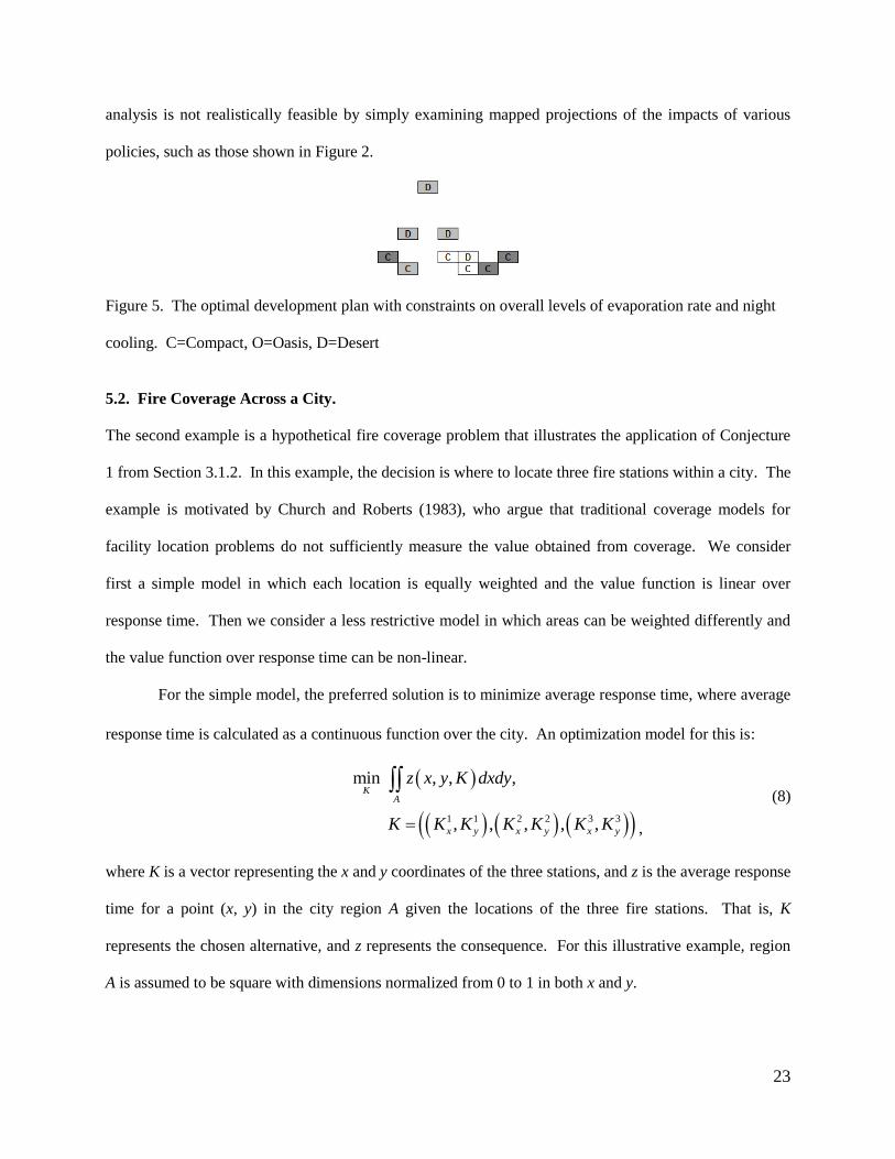
For the simple model, the preferred solution is to minimize average response time, where average

response time is calculated as a continuous function over the city. An optimization model for this is:

1 1 2 2 3 3

min , , ,

, , , , ,

KA

x y x y x y

z x y K dxdy

K K K K K K K

,

(8)

where K is a vector representing the x and y coordinates of the three stations, and z is the average response

time for a point (x, y) in the city region A given the locations of the three fire stations. That is, K

represents the chosen alternative, and z represents the consequence. For this illustrative example, region

A is assumed to be square with dimensions normalized from 0 to 1 in both x and y.

24

To develop a specific functional form for (8), we assume that for some fraction of incidents α, the

fire station assigned to respond is not the closest one. Of those incidents, the same fraction α are not

assigned to the next closest station. Finally, of those incidents not assigned to the two closest stations, the

same fraction α will end up unassigned to any of the three stations. With these assumptions, the average

response time used in equation (8) becomes:

3

1 3

1

, , 1 , ,ii

i

z x y K f d x y K f

, (9)

where K(i)

is the location of the ith closest station, , ,i

d x y K is the distance between (x,y) and K(i)

,

f(d) is the average response time from a station at distance d, and f is the average "unassigned" response

time (occurring when none of the three stations is properly equipped to respond). For d(·), we use a

“metropolitan” distance measure, which is the sum of the x and y distances to account for travel along

gridlines in a metropolitan area. The range of f(d) is assumed to be [0,1]. We assume that f(d) is linear in

d below an upper bound d'. We can think of d' as a large enough distance between the station and the

incident such that there is no benefit to responding, and the station therefore will not respond if d ≥ d'.

Provided α is not large, 3 f will be close to zero. Since this term is constant and close to zero, the exact

choice of f is immaterial, and we assume 3 f can be ignored. In this illustrative example, we set α =

0.15. While (9) was developed directly from the definition of average response time, the use of (8) is a

non-discrete special case analogous to (2) where all locations are given equal weight so that a(x, y) = 1 for

all x and y, and v(z) = z, and we will now generalize (8) based on Conjecture 1.

Given the relationship between response time and the size of the fire that the responder will have

to fight, it is reasonable to assume there are diminishing returns for decreases in response time from the

perspective of a policy maker. That is, high values will be placed on the range of response times which

will likely assure the survival of the building(s), while changes in response times slightly above this range

will be associated with steeper decreases in value. For example, assume the conditions specified in

25

Section 4.1 are met for an exponential value function to be valid and that the assessed tradeoffs midvalue

for the range from zero to one is 0.826, which results in the following single-attribute value function:

3.86 1 , ,

3.86

1, ,

1

z x y Ke

v z x y Ke

. (10)

Equation (10) is shown in Figure 6, normalized so that v(0) = 1 and v(1) = 0.

Figure 6. The exponential value function over average response time, with exponential constant c = 3.86.

It is reasonable that a rapid average response time could be more critical in some areas than

others, due to differences in, for example, population or economic importance. In such a case, the weight

( , )a x y will vary with x and y. Conceptually, the process in Section 4.2 to assess this weighting function

applies, but there are an (uncountably) infinite number of locations for which weights have to be

determined, so it is not practical to assess weights for each individual location. Two approaches are

practical in this situation: assess weights for a finite number of locations and use a curve fitting method to

fit a surface to these points, or assume a specified functional form for ( , )a x y that has a small number of

unspecified parameters, and assess the weights at enough locations to determine those parameters. There

is no existing theory to specify preference conditions that determine a functional form for ( , )a x y in the

way that there is theory to determine when an exponential single-attribute value function is valid. Thus,

we will show how such an approach might be used in a practical decision situation, such as the fire station

location decision.

26

For illustrative purposes, assume that development in this city is concentrated along a river

extending in a straight line upstream from near the center of the eastern boundary of the city, which is on

a bay, to near the southwestern corner, and that the decision maker wants more emphasis placed on

protecting areas which are closer to the bay and the river. Using the approach in Section 4.2, suppose that

the decision maker most prefers the hypothetical consequence with the best response time occurring at a

location near to the mouth of the river, but slightly inland. Also, assessing indifference relationships for

other locations determines that the decision maker wants the weight to decrease with increasing distance

from the most preferred location, and also wants the weight for areas along the river to be higher than

areas further away from the river for any specified distance from the bay. In addition, the decision maker

is unconcerned about the response times at the very edges of the city. The surface shown in Figure 7 has

these qualitative characteristics for the weighting function, and these characteristics could be modeled

quantitatively using a combination of beta-distribution functional forms for the x and y dimensions. While

there is not a theoretical justification for using this form, it fits the qualitative characteristics of the

decision maker's preferences, and we will use it to illustrate how a functional form can be used to specify

( , )a x y . (In this illustrative analysis, we ignore the impact of the river on response times.)

More specifically, we assume that the value function is specified as the product of an

unconditional marginal beta distribution for the x-variable and a conditional marginal beta distribution for

the y-variable, where the conditioning is through a straight-line equation for the mode of the y-variable

marginal beta distribution as a function of the x-variable. Based on the qualitative characteristics

presented in the preceding paragraph, the straight line that will be used is the course of the river. Using

this specification for the value function, the combined beta function is determined by five parameters: the

p and q parameters for the marginal distribution over x, the two parameters that determine the equation for

the mode line for the marginal distribution over y as a function of x, and one other parameter that can be

used along with the equation of the mode line to determine the p and q parameters of the conditional

marginal distribution over y. In addition, an equation must be specified to set the scaling for the

27

weighting function (for example, to ensure that it integrates to one over the region of interest), but that

does not require an assessment to determine.

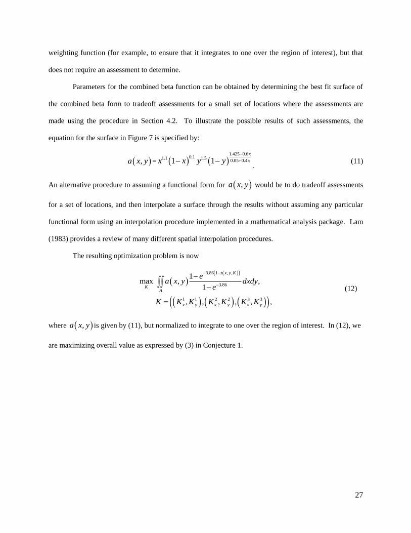
Parameters for the combined beta function can be obtained by determining the best fit surface of

the combined beta form to tradeoff assessments for a small set of locations where the assessments are

made using the procedure in Section 4.2. To illustrate the possible results of such assessments, the

equation for the surface in Figure 7 is specified by:

,a x y = 1.425 0.6

0.11.1 1.50.05 0.41 1

x

xx x y y

. (11)

An alternative procedure to assuming a functional form for ,a x y would be to do tradeoff assessments

for a set of locations, and then interpolate a surface through the results without assuming any particular

functional form using an interpolation procedure implemented in a mathematical analysis package. Lam

(1983) provides a review of many different spatial interpolation procedures.

The resulting optimization problem is now

3.86 1 , ,

3.86

1 1 2 2 3 3

1max , ,

1

, , , , , ,

z x y K

KA

x y x y x y

ea x y dxdy

e

K K K K K K K

(12)

where ,a x y is given by (11), but normalized to integrate to one over the region of interest. In (12), we

are maximizing overall value as expressed by (3) in Conjecture 1.

28

0.0

0.2

0.4

0.6

0.8

1.0

0.0 0.2 0.4 0.6 0.8 1.0

Continuous Weighting Function

Figure 7. A contour map of the illustrative weighting function expressing the weight assigned to any

point in the city. The maximum weight is assigned to (0.85, 0.4).

The optimization problems in (8) and (12) were solved numerically using a grid search with a

distance of 0.025 between adjacent points, and a numerical integration that divides the region into 400

cells, computing the average response time in the center of each cell. Changes in the search and

integration parameters did not noticeably affect the results. Figure 8 shows the optimal fire station

locations for (12) designated with diamonds, along with the locations determined by the unweighted

linear value function in (8) designated with circles. Conforming with the preference to protect areas

closer to the bay and river, the locations of the fire stations have been “pulled” toward the higher

weighted part of the city compared to their locations when only average response time is considered.

0.00

0.25

0.50

0.75

1.00

0.00 0.25 0.50 0.75 1.00

y

x

Optimal Fire Station Locations

Min. Avg. Time

Max. Value

Figure 8. Optimal fire station locations when minimizing unweighted average response time, and when

maximizing a geographically-weighted nonlinear value function.

29

6. Extensions of the Preference Models to Address Uncertainty

This section, included as Appendix F, discusses preference models for decisions where the consequences

of alternatives are uncertain, and addresses what conditions are needed for such models.

7. Concluding Comments

This paper presents preference models for decisions based on GIS data. As shown by the illustrative

hypothetical applications in this paper, these types of decisions are important in a variety of decision

contexts, and with the widespread use of GIS, it is now practical to apply more rigorous decision analysis

methods to these decisions. When faced with a decision that has consequences that can vary over a

geographic region, formulating specific structures and conditions for the decision stakeholders’

preferences will allow an analyst to elicit an appropriate value or utility function using the results in this

paper. This can help to provide a more defensible gauge of the desirability of the proposed decision

alternatives. We believe the methods in this paper can be applied to a wide range of real-world policy

decisions with geographically varying consequences, such as regional development planning, pollution

abatement, facility location, and utility service provision.

Electronic Companion. An electronic companion, containing the Appendices to this paper, is available

as part of the online version at http://dx.doi.org/10.1287/opre.xxxx.xxxxec. (still to be set up)

Acknowledgements. We were supported in part by a dissertation grant from the National Science

Foundation to UC Irvine and grants by the NSF-funded Decision Center for a Desert City at Arizona State

University under NSF award number SES-0345945. We thank the area editor, associate editor, two

reviewers, and participants in several conference and university session talks for providing valuable and

detailed comments that have resulted in substantial improvements to the paper. One reviewer provided

especially substantial assistance in improving our theoretical discussion.

30

References

Arbia, G. 1993. The Use of GIS in Spatial Statistical Surveys. International Statistical Review 61(2) 339-

359.

Bond, D., P. Devine. 1991. The Role of Geographic Information Systems in Survey Analysis. The

Statistician 40(2) 209-216.

Chan, Y. 2005. Location, transport and land-use: modelling spatial-temporal information. Springer.

Berlin; NY.

Church, R. L., K. L. Roberts. 1983. Generalized Coverage Models and Public Facility Location. Papers

in Regional Science 53(1) 117-135.

de Silva, F. N., R. W. Eglese. 2000. Integrating Simulation Modelling and GIS: Spatial Decision Support

Systems for Evacuation Planning. The Journal of the Operational Research Society 51(4) 423-430.

Debreu, G. 1954. Representation of a Preference Ordering by a Numerical Function. In Decision

Processes, 1954, R. M. Thrall, C. H. Coombs, and R. L. Davis (eds.), Wiley, New York, pp. 159-165.

Debreu, G. 1964. Continuity Properties of Paretian Utility. International Economic Review 5(3) 285-293.

Eisenführ, F., M. Weber, T. Langer. Rational Decision Making. Springer-Verlag, Berlin, 2010.

Fishburn, P. C. 1965. Independence in Utility Theory with Whole Product Sets. Operations Research,

13(1) 28-45.

Fishburn, P. C. 1970. Utility Theory for Decision Making. John Wiley and Sons, New York.

Gober, P., A. J. Brazel, R. Quay, S. Myint, S. Grossman-Clarke, A. Miller, and S. Rossi. 2010. Using

Watered Landscapes to Manipulate Urban Heat Island Effects: How Much Water Will It Take to Cool

Phoenix? Journal of the American Planning Association 76(1) 109-121.

Gorman, W. M. 1968. The Structure of Utility Functions. Review of Economic Studies 35(4) 367-390.

Harvey, C. M. 1986. Value Functions for Infinite-period Planning. Management Science 32(9) 1123-

1139.

31

Harvey, C. M. 1995. Proportional Discounting of Future Costs and Benefits. Math. of Oper. Res. 20(2)

381-399.

Jankowski, P. 1995. Integrating GIS and Multiple Criteria Decision Making Methods. International

Journal of Geographical Information Systems 9(3) 251-273, also reprinted in P. Fisher (Ed.), 2007,

Classics from IJGIS: Twenty Years of the International Journal of Geographic Information Science

and Systems 265-290. Boca Raton, FL: Taylor & Francis Group.

Jankowski, P. 2006. Integrating GIS and Multiple Criteria Decision Making Methods: Ten Years After. In

P. Fisher (Ed.), 2007, Classics from IJGIS: Twenty Years of the International Journal of Geographic

Information Science and Systems 291-296. Boca Raton, FL: Taylor & Francis Group.

Keefer, D. L., C. W. Kirkwood, J. L. Corner. 2004, Perspective on Decision Analysis Applications, 1990-

2001. Decision Analysis 1(1) 4-22.

Keeney, R. L. 1992. Value-focused Thinking: A Path to Creative Decisionmaking. Harvard Univ. Press,

Cambridge, MA.

Keeney, R. L., H. Raiffa. 1976. Decisions with Multiple Objectives: Preferences and Value Trade-offs.

John Wiley and Sons, New York, and Cambridge University Press, New York.

Keisler, J. M., R. C. Sundell. 1997. Combining Multi-Attribute Utility and Geographic Information for

Boundary Decisions: An Application to Park Planning. J. of Geographic Information and Decision

Analysis 1(2) 100-119.

Keller, L. R., C. W. Kirkwood, N. S. Jones. 2010. Assessing Stakeholder Evaluation Concerns: An

Application to the Central Arizona Water Resources System. Systems Engineering 13(1) 58-71.

Kirkwood, C. W. 1997. Strategic Decision Making: Multiobjective Decision Analysis with Spreadsheets.

Duxbury Press, Belmont, CA.

Kirkwood, C. W., and R. K. Sarin. 1980. Preference Conditions for Multiattribute Value Functions.

Operations Research 28(1) 225-232.

Knox, J. W., E. K. Weatherfield. 1999. The Application of GIS to Irrigation Water Resource Management

in England and Wales. The Geographical Journal 165(1) 90-98.

32

Kohlin, G., P. J. Parks. 2001. Spatial Variability and Disincentives to Harvest: Deforestation and

Fuelwood Collection in South Asia. Land Economics 77(2) 206-218.

Koller, D., P. Lindstrom, W. Ribarsky, L. F. Hodges, N. Faust, G. Turner. 1995. Virtual GIS: A Real-

Time 3D Geographic Information System. Proceedings of the 6th IEEE Visualization Conference 94-

100.

Krantz, D. H., R. D. Luce, P. Suppes, A. Tversky. 1971. Foundations of Measurement, Volume I:

Additive and Polynomial Representations, Academic Press, New York and London.

Lam, N. S. N. 1983. Spatial interpolation methods: a review. Cartography and Geographic Information

Science 10(2) 129-150.

Malczewski, J. 1999. GIS and Multicriteria Decision Analysis. Wiley. Hoboken, NJ.

Obermeyer, N. J., J. K. Pinto. 2007. Managing Geographic Information Systems. Guilford Press. New

York, NY.

Pendleton, G. W., K. Titus, E. DeGayner, C. J. Flatten, R. E. Lowell. 1998. Compositional Analysis and

GIS for Study of Habitat Selection by Goshawks in Southeast Alaska. Journal of Agricultural,

Biological, and Environmental Statistics 3(3) 280-295.

Slocum, T. A., C. Blok, B. Jiang, A. Koussoulakou, D. R. Montello, S. Fuhrmann, N. R. Hedley. 2001.

Cognitive and Usability Issues in Geovisualization. Cartography and Geographic Information Science

28(1) 61-75.

Worrall, L., D. Bond. 1997. Geographical Information Systems, Spatial Analysis and Public Policy: The

British Experience. International Statistical Review 65(3) 365-379.

S-1

e – companion ONLY AVAILABLE IN ELECTRONIC FORM

Electronic Companion—“Decision Analysis with Geographically Varying Outcomes: Preference Models

and Illustrative Applications” by Jay Simon, Craig W. Kirkwood, and L. Robin Keller, Operations

Research, http://dx.doi.org/10.1287/opre.xxxx.xxxx. (citation information)

______________________________________________________________________________

E – companion to: Decision Analysis with Geographically Varying Outcomes:

Preference Models and Illustrative Applications

Jay Simon

* Craig W. Kirkwood

† L. Robin Keller

‡

APPENDIX A: PREFERENTIAL INDEPENDENCE.

In decision analysis, specifying a multiattribute value or utility function requires assessments from a

decision maker, and this can be difficult because it requires the determination of an n-dimensional

function. To simplify this, researchers have established conditions on preferences under which the form

of the value or utility function is simplified. One of these conditions is preferential independence. A

subset of 1 2, , nZ Z Z , when 3n , is defined to be preferentially independent of its complement if the

rank ordering of alternatives with no uncertainty that have common levels for the complementary

attributes does not depend on those common levels. If this property holds for all subsets of

1 2, , , nZ Z Z , then mutual preferential independence is said to hold, and in this case

1 2

1

( , , , ) ( )n

n i i i

i

V z z z a v z

, (A-1)

* Defense Resources Management Institute, Naval Postgraduate School, Monterey, CA 93943, jrsimon@nps.edu

† W. P. Carey School of Business, Arizona State University, Tempe, AZ 85287-4706, craig.kirkwood@asu.edu

‡ The Paul Merage School of Business, University of California, Irvine, CA 92697-3125, LRKeller@uci.edu

S-2

where vi(zi) is called the single attribute value function over zi, and 0ia is called the weighting constant

for the ith attribute (Debreu 1960). Gorman (1968) derives several conditions related to mutual

preferential independence. In particular, it follows from his results that if every pair of attributes is

preferentially independent of the remaining attributes then mutual preferential independence holds, or,

even more specifically, if {Zi, Zi+1} is preferentially independent of its complement for i = 1, 2, …, n-1,

then mutual preferential independence holds. These results can substantially reduce the number of

assessments that must be made in applications to establish that (A-1) is valid. See Keeney and Raiffa

(1976 Sections 3.6.2- 3.6.4) for more details.

APPENDIX B: ADDITIONAL DISCUSSION OF THEOREM 1.

Let ~ (“at least as preferred as”) be a preference relation over Z , which is the set of possible

consequences (where a consequence is a vector of levels across all subregions), with the corresponding

strict relation (“more preferred than”) and indifference relation ~ (“equally preferred to”). Let q, r,

and s denote arbitrary vectors in Z . For z Z , we define i

z as the vector of attribute levels in all

subregions except subregion i, and ijz as the vector of attribute levels in all subregions except subregions

i and j.

Consider the following conditions on ~ :

(a) Completeness: It must be true that q ~ r or r ~ q. (That is, any consequences can be compared.)

(b) Transitivity: If q ~ r and r ~ s, then q ~ s.

(c) Continuity: If q r, then there exists 0 such that for any z Z , max i ii

z q implies

z r, and max i ii

z r implies q z.

(d) Dependence on each subregion: For each subregion i, there exist ,i iq z and ,i i

r z such that

S-3

, ,i ii iq rz z .

(e) Pairwise spatial preferential independence: For any two subregions i and j, ~, , , ,i j i jij ij

q q r rs s

for some ij

s implies ~, , , ,i j i jij ij

q q r rz z for all ij

z , z Z .

This condition implies mutual preferential independence, as described above. Since the independence

described here is for a single attribute across multiple subregions, it is labeled “spatial” to distinguish it

from preferential independence across multiple attributes, which is considered in Theorem 2.

DEFINITION A-1. An attribute level midz is called a tradeoffs midvalue of 'z and ''z in subregion i if

there exist vectors i

q and i

r such that ', ,mid

i iz z~q r and , '',mid

i iz z~q r .

(f) Homogeneity: If midz is a tradeoffs midvalue of 'z and ''z in subregion i, then for any subregion j

and vectors j

q , j

r such that ', ,mid

j jz z~q r it must be true that , '',mid

j jz z~q r . (An

equivalent definition is that when two amounts z, z’ have a tradeoffs midvalue in a subregion i and also in

a subregion j, then they have the same tradeoffs midvalue in subregion i as in subregion j.)

A value function exists over the set of consequences if and only if ~ is complete, transitive, and

continuous, as specified in conditions (a)-(c). (This is a special case of Debreu (1954, 1964), who uses a

more general topological space.) It follows directly from Debreu’s (1960) theorem that for a region with

three or more subregions, a value function can be written as:

1 2

1

( , , , ) ( )m

m i i i

i

V z z z a v z

(A-2)

if and only if conditions (a)-(e) above hold, where vi is a single attribute value function over iz , and

0ia is the weight associated with subregion i. While (A-2) has the same form as (A-1), the iz in (A-

2) represent the levels of the same attribute in different subregions, rather than the levels of different

attributes 1 2, , , nZ Z Z as in (A-1). Harvey (1986, p. 1126, Condition E) defines the Equal Tradeoffs

S-4

Comparisons condition, and he notes that a condition that is mathematically equivalent to homogeneity

(our condition (f)) is equivalent to his Equal Tradeoffs Comparisons condition. He then shows (Harvey,

1986, p. 1136-37, proof of Theorem 1) that an intertemporal analog of (1) is a valid representation of

preferences if and only if (A-2) and his condition E hold. Since his Condition E is equivalent to our

condition (f), that proof also establishes our Theorem 1.

Value functions are only determined to within a positive monotonic transformation, so any

positive monotonic transformation of the value function forms in all of the Theorems and Conjectures

will also satisfy the specified conditions. See Keeney and Raiffa (1976, Section 3.3.4) and Kirkwood

(1997, Section 9.2) for further discussion of this point.

With a stronger condition in place of condition (f), a special case of equation (1) holds where

( )iv z is linear. Consider the stronger condition of tradeoffs neutrality: for any subregion i, attribute

levels iz and iz , and vectors i

q and i

r , *, ,i i iz z ~q r , implies *, ,ii i

z z~q r , where

* 0.5 i iz z z . This condition ensures that single-attribute value functions will be linear by the

following argument: Since tradeoffs neutrality is a special case of condition (f), equation (1) still holds in

this case. By direct substitution, when tradeoffs neutrality holds, [0.5 ( )] 0.5 [ ( ) ( )]i i i iv z z v z v z

for any iz and iz . This is Jensen’s equation (Small, 2007, Section 2.3), and the solution is

( )v z az b for constants a and b when ( )iv z is continuous.

(An anonymous reviewer provided valuable suggestions that helped us to develop the material

just presented in this section. This same reviewer also provided many valuable suggestions for the other

theorem and conjecture presentations in this Appendix.)

APPENDIX C: ADDITIONAL DISCUSSION OF CONJECTURE 1.

Let ~ have corresponding strict and indifference relations as previously defined, and let q, r, and

s denote arbitrary consequences. Consider the following conditions on ~ :

S-5

(a’) Completeness: It must be true that q ~ r or r ~ q. (That is, any consequences can be compared.)

(b’) Transitivity: If q ~ r and r ~ s, then q ~ s.

(c’) Continuity: If q r, then there exists 0 such that for any consequence z ,

,

max , ,x y

z x y q x y implies z r, and ,

max , ,x y

z x y r x y implies q z.

(d’) Dependence on any subregion: For any proper subregion of the region with area greater than

zero, there exist consequences q and r such that , ,q x y r x y= for all ,x y , and q r.

(e’) Spatial preferential independence: For any proper subregion of the region with area greater than

zero, if there exist consequences q, r, q', and r' such that q~

r, , ,q x y q x y =

and

, ,r x y r x y = for all ,x y , and , ,q x y r x y= and

, ,q x y r x y = for all

,x y , then it must be true that q'~

r'.

DEFINITION A-2. Consider a proper subregion of the region with area greater than zero, and consider

two consequences ),( yxz and ),( yxz

that have constant levels z and z , respectively, within P. An

attribute level midz

is a tradeoffs midvalue for z and z with respect to P if there exist functions

( , )q x y and ( , )r x y

defined outside P such that the following two indifference relations hold: i) a

consequence that is equal to z within P and equal to ( , )q x y outside P is indifferent to a consequence

that is equal to midz within P and equal to ( , )r x y outside P, and ii) a consequence that is equal to

midz

within P and equal to ( , )q x y outside P is indifferent to a consequence that is equal to z within P and

equal to ( , )r x y outside P.

S-6

(f’) Homogeneity: If midz is a tradeoffs midvalue for z and z with respect to a specified proper

subregion P of the region with area greater than zero, then it is also a tradeoffs midvalue for z and z

with respect to any other proper subregion for which a tradeoffs midvalue for z and z exists.

Note that tradeoffs midvalues are unlikely to exist with respect to very large subregions, since the

required ( , )q x y and

( , )r x y

may not exist for such cases. However, for the purposes of both practical

applications and possible proofs of Conjecture 1, we are concerned only with subregions which are small

relative to the entire region.

We present a plausibility argument for why conditions (a’) through (f’) might imply (3), and

discuss where difficulties arise in the proof. The conditions stated in Conjecture 1 are analogous to those

used in Theorem 1, and (3) is analogous to (1). Conditions (a’)-(e’) are straightforward adaptations of

conditions (a)-(e). (Condition (e’) is analogous to mutual preferential independence, rather than pairwise

preferential independence, because in the non-discrete case there are not existing discrete subregions with

which to create pairs.) Condition (f’) is analogous to condition (f).

To establish the plausibility of Conjecture 1, start with (1) and define iii Aa / in (1),

where iA is the area (for example, in square miles) of subregion i. Then (1) can be rewritten as

m

i

iiim zvAzzzV1

21 )(),,,( . (A-3)

Since conditions (a’) through (f’) are analogous to conditions (a) through (f) required for (1), it is

plausible to use (1) as a starting point for developing (3). Extend (A-3) to an attribute that varies over the

region as follows: Partition the region into a uniform grid, where the two dimensions of the grid are

designed by x and y, and where the x and y dimensions of each cell in the grid are designated

by x and y , respectively, so that the area iA of any cell is yx . While it is easiest to visualize

this partition if A is rectangular, the analysis can be extended to any region that is bounded by a piecewise

smooth curve, as established in the references given below. If i and )( ii zv did not vary within a grid

cell, then if the assumptions for Theorem 1 are assumed to hold, (A-3) can be written as

S-7

m

i

iiiim yxyxzvyxzzzV1

21 )],([),(),,,( , (A-4)

where ix and iy designate some specified but arbitrary point within grid cell i, iii yx ),( , and

)()],([ iii zvyxzv . Equation (A-4) has the form of a special case of a Riemann sum of

)],([),( yxzvyx over A, and if and v are both bounded, then their product is also bounded. If these

functions are continuous almost everywhere (that is, except on a subset of A with measure zero), then

)],([),( yxzvyx is Riemann integrable over A if the boundary of A is a piecewise smooth curve. (For

proofs of this, see Apostol 1962, Section 2.12, or Trench 2003, Theorem 7.1.19.) If )],([),( yxzvyx is

integrable, the Riemann sum in (A-4) will converge to a unique value (which by definition is the integral)

as the partition of A is made finer so that m approaches infinity and both x and y approach zero.

Thus, in the limit, (A-4) would become

( ) ( , ) [ ( , )]A

V z x y v z x y dxdy , (A-5)

where V(z) is the value from a decision-making perspective associated with the distribution of the

attribute over the region of interest. The converse of the model result would follow by direct substitution

from (3). Note that in (3), ),( yx in (A-5) has been replaced with a(x, y) to make the notation more

parallel to (1). However, the units for a in (1) and (3) are different.

The plausibility argument given above is not a proof, and there are two primary difficulties

involved in proving Conjecture 1. The first is that the partition of the region used in (1) is fixed, as is the

number of subregions. Therefore, we cannot be sure that assessed preferences for different partitions,

such as the changing partitions in (A-4) as m increases, will yield the same single-subregion value

function v, and hence yield a single common limit for any possible Riemann sum. This means it is not

defensible to examine the limit of (1) as m goes to infinity, because a common limit of ( )iv z independent

of the partition is not guaranteed to exist. In the conditions for Conjecture 1, we address this with the

S-8

continuity condition (c’). While this is meant to guarantee convergence as the partition becomes finer, we

cannot establish that it does this in the manner required for a unique limit to exist.

A second difficulty is establishing that the weighting function ,a x y is Riemann integrable. It

must be true that [ ( , )]v z x y is Riemann integrable, because ( , )z x y is Riemann integrable by

assumption, and conditions (c’) and (d’) ensure that v is continuous and bounded. The weighting function

must be bounded, otherwise a violation of condition (d’) would occur. However, it must also be

established that the weighting function is continuous almost everywhere, and it is not clear precisely what

conditions on the preference relation will guarantee this. Condition (c’) establishes the continuity of v,

but does not impose this property on ,a x y . In practical applications, it is difficult to think of a

realistic weighting function that is not continuous almost everywhere, but we are unable to prove that

conditions (a’) through (f’) establish this property.

Harvey and Østerdal (2011) provide additional discussion of the steps necessary to establish a

result analogous to (3) in the context of continuous time decisions.

APPENDIX D: ADDITIONAL DISCUSSION OF THEOREM 2.

We thank a reviewer for pointing out that the result in Theorem 2 can be developed in either of two ways:

By using results from Gorman (1968) and then applying homogeneity conditions, or by applying

preferential independence conditions across attributes to Harvey’s (1995) value model. We use the

former approach here.

Modify the notation presented earlier so that iZ now designates the vector of n attributes

inii ZZZ ,,, 21 in subregion i (referred to as the “attribute vector for subregion i”), and j

Z designates

the vector mjjj ZZZ ,,, 21 of the jth attribute across the m subregions (referred to as the “subregion

vector for attribute j”), where iz and j

z are vectors of specific levels of iZ and j

Z , respectively. Let

~ have corresponding strict preference and indifference relations as previously defined, and let q, r, and s

S-9

denote arbitrary consequences. Consider the following conditions on ~ , which are analogous to those

used in Theorem 1.

(a’’) Completeness: It must be true that q ~ r or r ~ q. (That is, any consequences can be compared.)

(b’’) Transitivity: If q ~ r and r ~ s, then q ~ s.

(c’’) Continuity: If q r, then there exists 0 such that for any z Z , ,

max ij iji j

z q implies

z r, and ,

max ij iji j

z r implies q z.

(d’’) Dependence on each attribute-subregion combination: For each subregion i and attribute j, there

exist consequences ,ij ijq z and ,ij ij

r z such that , ,ij ijij ijq rz z .

(e”) Preferential independence:

1) Subregion preferential independence: For any subregion i, ~

, ,i ii iq s r s for some

is implies

~

, ,i ii iq z r z for all

iz , and

2) Attribute preferential independence: For any attribute j, ~, ,j j j j

q s r s for some j

s implies

~, ,j j j j

q z r z for all j

z .

DEFINITION A-3. Preferences over the region of interest with respect to a set of attribute vectors

1, , mZ Z for subregions 1, …, m are multiattribute homogeneous if, when two alternatives that differ

only in the attribute levels for a specified subregion are indifferent, then the same indifference relation

holds for those same attribute levels in any subregion. (In this definition, the scalar attribute for each

subregion considered in Theorem 1 is replaced with an attribute vector for each subregion).

(f’’) Homogeneity: ~ is multiattribute homogeneous with respect to 1, , mZ Z .

Condition (f’’) plays a role for multiple attributes similar to the single-attribute homogeneity

condition (f) previously defined for Theorem 1. Condition (f) assumes there is a single attribute that has a

S-10

tradeoffs midvalue, but when there are multiple attributes there is not an unambiguous meaning for the

tradeoffs midvalue. Therefore, we express homogeneity here considering levels of multiple attributes.

Conversely, the definition given here requires considerations of tradeoffs between attributes, and

therefore is not applicable to the single-attribute consequences used in Theorem 1.

We first show that condition (e”) implies an additive form for ( )V z . The first step is to show

that the set consisting of any pair of attribute-subregion combinations is preferentially independent of its

complement. Let acZ and bdZ represent two such combinations, where a and b are arbitrary distinct

subregions, and c and d are arbitrary distinct attributes. From condition (e”), each of aZ , bZ , c

Z , and

dZ is preferentially independent of its complement. From Theorem 1 in Gorman (1968), the union of

aZ and d

Z is preferentially independent of its complement, as is the union of bZ and c

Z . The

intersection of these two unions is ,ac bdZ Z , and since both unions are preferentially independent of

their complements, Theorem 1 in Gorman also implies that ,ac bdZ Z must be preferentially independent

of its complement. Since the choices of a, b, c, and d were arbitrary, any pair of attribute-subregion

combinations is preferentially independent of its complement for distinct attributes and subregions. It is

then straightforward to also use Theorem 1 in Gorman to show that a pair of attribute-subregion

combinations is preferentially independent of its complement in the case where either the attribute or the

subregion is common to both combinations. Hence, from inductive application of Gorman's results, also

stated as a Corollary on page 114 of Keeney and Raiffa (1976), the ijZ are mutually preferentially

independent, and therefore:

1 1

( ) ( )m n

ij ij ij

i j

V z k v z

. (A-6)

Since the attributes are multiattribute homogeneous by condition (f’’), it follows from an analogous

argument to the one given in the proof of Theorem 1 that single-attribute value functions ijv cannot

depend on the subregion i, and hence the following equation holds in this case:

S-11

1 1

( ) ( )m n

ij j ij

i j

V z k v z

. (A-7)

To show that jiij bak , and hence (4) holds, first assume without loss of generality that the

subregions and attributes are labeled so that the largest scaling constant is 11k . Consider two hypothetical

alternatives: 1) all the attribute-subregion combinations except 11Z and jZ1 are set to arbitrary levels,

11Z is set to its least preferred level so that 0)( 111 zv in (A-7), and jZ1 is set to its most preferred level

so that 1)( 1 jj zv , and 2) another hypothetical alternative with all the attribute-subregion combinations

except 11Z and jZ1 set to the same arbitrary levels as the first alternative, jZ1 set to its least preferred

level so 0)( 1 jj zv , and 11Z set to the level jz11 such that the two alternatives are equally preferred.

Then equating the values for each of these two alternatives calculated using (A-7) and cancelling common

terms results in j

j kzvk 111111 )( for any 1j . However, by condition (f’’), if this equation holds for

subregion 1, then the same level jz11 must make the analogous equation true for any subregion i, and

hence ij

j

i kzvk )( 1111 for any i. Define )( 111

j

j zvb and 1ii ka . Substituting these definitions into

ij

j

i kzvk )( 1111 gives jiij bak . Substitute this into (A-7), and (4) follows. The converse of the model

result follows by direct substitution from (4).

APPENDIX E: ADDITIONAL DISCUSSION OF CONJECTURE 2.

Let ~ have corresponding strict and indifference relations as previously defined, and let q, r, and

s denote arbitrary consequences. Let jz designate a Riemann integrable function such that

,j jz x y I for all ,x y in the region. Let j

z and ijz be defined as previously. As in Conjecture 1,

assume that the boundary of the region is a piecewise smooth curve. Consider the following conditions

on ~ , which are analogous to those used in Theorem 2:

S-12

(a’’’) Completeness: It must be true that q ~ r or r ~ q. (That is, any consequences can be compared.)

(b’’’) Transitivity: If q ~ r and r ~ s, then q ~ s.

(c’’’) Continuity: If q r, then there exists 0 such that for any consequence z ,

, ,

max , ,j j

x y jz x y q x y implies z r, and

, ,max , ,j j

x y jz x y r x y implies q z.

(d’’’) Dependence on any attribute in any subregion: For any attribute j and proper subregion of the

region with area greater than zero, there exist consequences q and r such that , ,j jx y x yq = r for all

,x y , , ,x y x yq = r for all ,x y , and q r.

(e’’’) Preferential independence:

1) Spatial preferential independence: For any proper subregion of the region with area greater

than zero, if there exist consequences q, r, q', and r' such that q~

r, , ,x y x yq = q and

, ,x y x yr = r for all ,x y , and , ,x y x yq = r and

, ,x y x y q = r for all

,x y , then it must be true that q'~

r'.

2) Pairwise attribute preferential independence: For any two attributes i and j,

~, , , ,i j ij i j ijq q r rs s for some

ijs implies ~

, , , ,i j ij i j ijq q r rz z for all ij

z .

DEFINITION A-4. Consider a proper subregion of the region with area greater than zero, and consider

two consequences q and r. Preferences over the region are continuously multiattribute homogeneous if

~q r , ( , ) ( , )x y x yq r for ( , )x y P , and 1( , ) , , nx y q qq and 1( , ) , , nx y r rr for

( , )x y P where 1, , nq q and 1, , nr r are constants implies that for any consequences z and z

and subregion such that ( , ) ( , )x y x y z z for ( , )x y P , and 1( , ) , , nx y q q z and

1( , ) , , nx y r r z for ( , )x y P then ~ z z .

(f’’’) : Homogeneity: ~ is continuously multiattribute homogeneous over the region.

S-13

The development of Conjecture 2 from Theorem 2 is analogous to the development of Conjecture

1 from Theorem 1. A similar plausibility argument can be given for Conjecture 2, in which a Riemann

sum analogous to equation (A-4) is developed. A further development analogous to the Conjecture 1

reasoning leads to (5), and direct substitution from (5) yields the converse of the result. However,

analogous difficulties to those involved in proving Conjecture 1 arise here as well.

APPENDIX F: EXTENSIONS OF THE PREFERENCE MODELS TO ADDRESS UNCERTAINTY.

In this Appendix, we examine the case in which the consequences of alternatives are uncertain. We

assume that probabilities can be assigned to the possible consequences of each alternative, and we wish to

rank alternatives by their overall desirability using their expected utility, computed as the expected value

of a single attribute (or multiattribute) utility function. The preference conditions in Section 3 can be

extended to decisions under uncertainty to determine the requirements for an additive utility function.

The primary difference is that the preferential independence condition discussed in Section 3 must be

replaced by a considerably stronger condition called additive independence.

DEFINITION A-5. Additive independence with respect to Z over the region of interest holds if the rank

ordering for any set of alternatives depends only on the marginal probability distributions for each

alternative over the levels z1, z2, …, zm of Z in each of the subregions 1, ..., m.

We first consider the case analogous to Theorem 1, in which the level for the single attribute Z does not

vary within each subregion, and then consider the non-discrete case analogous to Conjecture 1.

In decision problems with uncertainty, we maximize expected utility using a utility function

instead of maximizing a value function. It is straightforward to show that utility is given by

1 2

1

( , , , ) ( )m

m i i

i

U z z z a u z

(A-8)

if and only if additive independence is satisfied, and conditions analogous to (a)-(d) and (f) in Appendix B

are met (Fishburn 1965). See Keeney and Raiffa (1976, Sections 6.5-6.6, pp. 295-307) and Kirkwood

(1997, pp. 249-50) for further background, including assessment procedures for utility functions.

S-14

Analogously to Conjecture 1, we conjecture that it is possible to extend (A-8) to situations where

the single attribute Z is defined at any location ( , )x y within the region of interest. The corresponding

utility function is given by:

( ) ( , ) [ ( , )]A

U z a x y u z x y dxdy (A-9)

if and only if additive independence, and conditions analogous to (a’)-(d’) and (f’) in Appendix C are met.

With these conditions, a plausibility argument for equation (A-9) can be obtained using reasoning

analogous to the discussion in Appendix C. However, as in Conjecture 1, this plausibility argument

would not constitute a proof. Results analogous to Theorem 2 and Conjecture 2, with a multiple attribute

utility function and analogous assumptions can also be specified.

The required preference assumptions for an additive utility function are strong, however, and may

not be appropriate in some decision situations. One possible approach to developing more general utility

function forms with less restrictive requirements would be to construct the utility function over the value

functions that were developed in Section 3 using methods such as those presented by Dyer and Sarin

(1982) and Matheson and Abbas (2005). If the conditions needed for a value function of the form given

in (1) hold, then in the case with discrete subregions, a utility function U could be constructed over the

value function in (1) with the form:

1 2

1

( , , , ) ( )m

m i i

i

U V z z z U a v z

. (A-10)

Similarly, in the non-discrete case, the utility function could be constructed over the value function in (3)

with the form:

( ) ( , ) [ ( , )]A

U V z U a x y v z x y dxdy

.

(A-11)

These are less restrictive than (A-8) and (A-9) in that they have unspecified utility functions U, and hence

require less restrictive preference conditions than (A-8) or (A-9). Standard utility function assessment

procedures can be modified to determine U. For example, a possible approach for assessing this utility

S-15

function is to identify the potential decision consequences with the highest and lowest possible values,

and visualize a hypothetical binary gamble between them with probability p of the highest-value

consequence occurring and probability 1-p of the lowest-value consequence occurring. The utility of the

value placed on a specified consequence could then be determined by finding the value of p for which the

decision maker is indifferent between the specified consequence and the gamble. By equating expected

utilities, the assessed p would be the utility associated with the specified consequence.

Additional References

Apostol, T. M. 1962. Calculus, Volume II: Calculus of Several Variables with Applications to

Probability and Vector Analysis, Blaisdell Publishing Company, New York.

Debreu, G. 1960. Topological Methods in Cardinal Utility Theory. In Mathematical Methods in the

Social Sciences, 1959, K. J. Arrow, S. Karlin, and P. Suppes (eds.), Stanford University Press,

Stanford, CA, 1960, pp. 16-26. Downloaded from http://cowles.econ.yale.edu/P/cp/p01b/p0156.pdf

on Nov. 29, 2010.

Dyer, J. S., R. K. Sarin. 1982. Relative Risk Aversion. Management Science 28(8) 875-886.

Harvey, C. M., L. P. Østerdal, 2011. Integral Utility Models for Outcomes over Continuous Time.

Working paper. Cited with permission of the authors.

Matheson, J. E., A. E. Abbas. 2005. Utility transversality: A value-based approach. Journal of Multi-

Criteria Decision Analysis 13(5-6) 229-238.

Small, C. G. 2007. Functional Equations and How to Solve Them, Springer Science+Business Media,

New York.

Trench, W. F. 2003. Introduction to Real Analysis. Pearson Education. Upper Saddle River, NJ. Free

Edition 1.05 downloaded on 11-29-10 from

http://ramanujan.math.trinity.edu/wtrench/texts/TRENCH_REAL_ANALYSIS.PDF.