, IResearch Report No. EES DA-79-5December 1979

(v)c0

Im

THE CONCEPT OF INFLUENCE AND ITS USE

IN STRUCTURING COMPLEX DECISION PROBLEMS

DANIEL L. OWEN DTICELECTEJUL 2 9 98?S.D

.DECISION ANALYSIS PROGRAM NN

Professor Ronald A. HowardPrincipal Investigator

DEPARTMENT OF ENGINEERING-ECONOMIC SYSTEMS

Stanford UniversityStanford, California 94305

SPONSORSHIP

Advanced Research Projects Agency, Cybernetics TechnologyOffice, Monitored by Engineering Psychology Programs,Office of Naval Research, contract No. N00014-79-C-0036.

_ _ __,

SAppe. " :io

0 J 2

SECURITY CLASSIFICATION OF THIS PAGE (_Whene DW.. E_ ____F__r__

READ INSTRUCTZONSREPORT DOCUMENTATION PAGE BEFORE COMPLETING FORM

P U. GOVT AC SSRONEO. RECIPIENT'S CATALOG NUMVIER

EES DA-79-5 F 1F4. TITLE land Subtitle) IS. TYPE OF REPORT & PERIOD COVERED

"The Concept of Influence and Its Use inStructuring Complex Decision Problems"

6. PERFORMING ORG. REPORT NUMBER

EES DA-79-57. AUTHOR(*) I. CONTRACT OR GRANT NUMEER(a)

Daniel L. Owen N00014-79-C-0036

9. PERFORMING ORGANIZATION NAME AND ADDRESS 10. PROGRAM ELEMENT. PROJECT. TASK

The Board of Trustees of the Leland Stanford AREA & WORK UNIT NUMBERS

Junior University, c/o Office of Research Admin-istrator, Encina Hall, Stanford, Ca. 94305

II. CONTROLLING OFFICE NAME AND ADDRESS III. RVPORT DATE

Advanced Research Projects Agency December 1979Cybernetics Technology Office 13. NuMSER Of PAGES

1400 Wilson Blvd., Arlington, Va. 22209 140t4. MONITORING AGENCY NAME 6 AOORESS(I•I dllermt lmP Cen-tre;Ind 0111c) 1S. SECURITY CLASS. (of thle report)

Engineering Psychology ProgramsOffice of Naval Research Unclassified800 No. Quincy St., Arlington, Va. 22217 r-0'. DECkhSIFICATI ON/OOWNRAOING

SCHEDULE

It. $ISTRI8UTION STATEMENT (of this Report)

Approved for public release. IDistribution unlimited.

I?. DISTRIBUTION STATEMENT (of the abstract entered In block 20. It different fom Repert)I

If. SUPPLEMENTARY NOTES

19, KEY WORDS (Contlnue en revaroe old& it necessary and Idan.ify by block number)

STRUCTURING DECISION ANALYSIS

MODELING INFLUENCE DIAGRAMS

20. ABSTRACT (Continue an reverse side if necessary end Identify by bolck number)

The generality of the decision analysis methodology permits itsapplication to decision problems regardless of the particular disciplineor setting in which the problem occurs. Consequently, the decision analystmay be unfamiliar with the relationships of the variables in the problem.One device for communicating those relationships is a diagram identifying

(continued)

DD I JAN7 1473 EOITION OF I NOV65IS OBSOLETE UnclassifiedSECURITY CLASSIFICATION OF THIS PA(.;E (W7hen Data Entered)

UnclassifiedS~Cu,'rY CLASSeI•,CATIYO- 0 THIS PAOC(Wh. Dote rnt.,.d)

the existence of influences between the variables. This researchcontributes a general mathematical characterizdtion of -the influencebetween random variables. The influence can be characterized by amatrix that is null if and only if no influence exists and otherwiseindicates the degree and type of influence by its nonzero elements.

An electrical engineer uses the schematic diagram of a circuitto conceptualize and communicate the relationship between the voltageat different points of an electronic device. The definition ofinfluence can serve the decision analyst in an analogous manner,helpii~g him to conceptualize and communicate the relationship of theprobability distributions on different variables in a probabilisticdecision model. The definition of influence supports a calculus ofinfluences that allows one to compute the total influence of onevariable on another even when there are several intermediateL

variables. Using this influence calculus, the importance of aparticular variable to the decision model can be determined. Animmediate consequence is a recommendation for which variables toinclude In the model and whether the uncertainty about a variable isimportant. These recommendations include a new interpretation ofdeterministic sensitivity.

An important, philnonphical result of this research is thedemonstration that which variables shouiu Le included in the decisionmodel depend on the decinn m_.or' rLt _ttit,,d• Two decisionmakers with the same state of information but different risk attitudesshould model the same decision problem differently.

Finally, the theoretical basis for the influence definition isdifferent from that of the conventional discretization or decisiontree representation for solving decision problems. Since theacceptability of the influence method depends on its accuracy andease of implementation relative to discretization, the theoreticalbases of the influence method and discretization are compared.

Accesiorn For

NTIS CRA&MI JDI IC TAB U

U!;dr:rnouficC'd 0J11-tificaot i ..... .... ......

B yi.t .. .. ..... ...... ........................ ...i-te :I- •

Availability Codes

UnclassifiedSICURITY CLASSIFICATION OF THIS PAGE')When Dole k.V.,ed)

• •16

%Copyright 1979

by

Daniel Owen

iii

Abstract

The generality of the decision analysis methodology

permits its application to decision problems regardless of

the particular discipline or setting in which the problem

occurs. Consequently, the decision analyst may be unfamiliar

with the relationships of the variables in the p~roblem. one

device for communicating those relationships is a diagram

identifying the existence of influences between the variables.

This research contributes a general mathematical characterization

of the influence between random variables. The influence can

be characterized by a matrix that is null if and only if no

influence exists and otherwise indicates the degree and type

of influence by its nonzero elements.

An electrical engineer uses the schematic diagram of a

circuit to conceptualize and communicate the relationship

between the voltage at different points of an electronic

device. The definition of ý*,ifluence can serve the decision

analyst in an analogous manner, helping him to conceptualize

and communicate the relatione'hip of the probability distribu-

tions on different variables in a probabilistiL. decision

model. The definition of influence supports a calculus of

influences that allows one to compute the total influence

of one variable on another even when there are several inter-

mediate variables. Using this influence calculus, the impor-

tance of a particular variable to the decision model can be

determined. An immediate consequence is a recommendatior for

iv

which variables to include in the model and whether th2 un-

certainty about a variable is important. These recommenda-

tions include a new interpretation of deterministic sensitiv-

ity.

An important, philosophical result of this research is

the demonstration that which variables should be included in

the decision model depend on the decision maker's risk atti-

tude. Two decision makers with the same state of information

but different risk attitudes should model the same decision

problem differently.

Finally, the theoretical basis for the influence defini-

tion is different from that of the conventional discretization

or decision tree representation for solving decision problems.

Since the acceptability of the influence method depends on its

accuracy and ease of implementation relative to discretiza-

tion, the theoretical bases of the influence method and dis-

cretization are compared.

v

"My master is so great because he eats when he is

hungry and drinks when he is thirsty."

part of a Buddhist Proverb

"Uncertainty makes me nervous, and certainty makes

me unnervous."

. . . Mary Hartman, Mary Hartmnan

vi

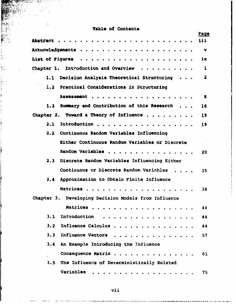
Table of Contents

Acknowledgements . . . . . . . . .. . . . . . . . . . . . v

List of Figur~es . . . . . . . . . . . . . . . . . . . . . ix

Chapter 1. Inritoduction and Overview . . . . . . . . . .1

* . ~1.3. Decision Analysis Theoretical Structuring . . 2

1.2 Practical Considerations in Structuring

Assessment... . . . . . . . . . . . . . . . . 8

1.3 Susuary and Contribution of this Research . . . 16

Catr2.1 Twr hoyo Intfoductio . . . .** . .** . . . 19

Catr2.1 Tvr hoyo Influedcetion . . . . . . 19

2.2 Contiuuous Random Variables Influencing

Either Continuous Random Variables or Discrete

Random Variables. ...... . ...... 20

2.3 Discrete Random Variables Influencing Either

Continuous or Discrete Random Varia±bles . . . . 35

2.4 Approximation to Obtain Finite Influence

Matrices . . . . . . . . . . . . .. ..... ... ... ... ......... 38

Chapter 3. Developing Decision Models from Influence

Matrices . . . . . . . . . . . . . . . . . . . 44

3.1 Introduction .. . . . . . . . . . . . . . . . 44

3.2 Influence Calculus . . . . . . . . . . . . . . . 44

3.3 Influence Vectors . *.*.. .. ............................. 57

3.4 An Example Introducing the Influence

Conseq en qMtrx nc.. .. at..rix. 61

3.5 The Influence of Deterministically Related

Variables . . . . . . 75

Vii

Chapter . A Comparison of the Quadratic

Apploximation with Discretization . . . . . . 89

4.1 ntoduatio . . . . . . . . . . .... 89

4.2 An Overview of Two Proposed Aisessment

Procedures . . . . .90

4.3 An Zxample Doenstrating the Two.

Quadratio Proceures .......... .. 94

4.4 Comparison of Discretization with

the Quadratic Approximation . . . . . . . . . .107

Chapter 5. Summary and Suggestion& for Further

Research . . . . .... . .... .. . 116

Reference8s . ....... . .... , ....... 121

Appendix A. A Series Representation and Approximation

for the Covariance ............ A-1

Appendix B. A Proof that the Change in Certain

Equivalent of (WIS .. ......... A-4

viii

List of Figures

1-1 A representation of the expansion equationshowing the sets S of state variables . . . . 4

1-2 Deterministic sensitivity for two variables . * 6

1-3 Communication paths required for struc-turing a complex decision problem . . . . . . . 10

1-4 The correspondence between influence dia-grams and assertions of probabilistic in-dependence . . . . . . . . . . . ..... . 11

1-5 Multiplication of interaction matrices . . . .. 14

1-6 An example demonstrating ambiguity aboutthe relative importance of two influences . . . 15

2-1 A comparison of our respresentation ofinfluence with the conventional repre-sentation ........ .. .. ... ... 33

2-2 An influence diagram suggesting an influencecalculus 4. . . 4. .. . 0. . . . .. . . .. . . 34

2-3 The effects of approximations on the in-fluence matrix ......... Va ..... 41

2-4 The elements of the approximate influencematrix for the influence of (xIS) on{YIS) . . . . . . . . . . . 0 * 0 * 0 0 43

3-1 Examples of the influence calculus usingthe procedure of Table 3-1 .. ........ . 47

3-2 An influence diagram with a direct and anindirect influence ..... 48

3-3 The elements of the influence matrices ofEquation (3.2.13) . . . . . . . . . . . . . . . 53,54

3-4 Two independent influences on a variable . . . . 56

3-5 An influence diagram with a direct and twoindirect influences . . . . . . . . . . . . . . 56

3-6 The elements of selected influence matricesof Equation (3.2.16) . . . . . . . . . . . . . . 58,59

ix

Page3-7 Influence for the modified entreprenuer's

problem . . . . . . . . . . . . . . 63

3-8 Dopendence of the conditional means andvariances for the modified entrepronuar'sproblem . . . . . . . . . . . . . . • . . ,. * . . 64

3-9 The influence matrices for the influencesof y , 8. and c. • • • • • . .. .... • . • . 66

3-10 The influence-consequence matrix . . . . . . . . . 70

3-11 The approximate influence matrix for deter-ministic influences . . . . . . . . . . . . . .. 76,77

3-12 Deterministic sensitivity for two variables . . . 78

3-13 Modeling policy diagram for treating thevariable x, or x 2 as uncertain on thebasis of their deterministic sensitivities .... 80

3-14 Deterministic sensitivity for a decisionanalysis example •....... • ..... 83

3-15 Functional forms for the deterministicsensitivities of xS, x6 , and x5 . ....... 85

3-16 Modeling policy diagram for treating thevariable x 5 or x 7 as uncertain showingthe location of the transfer price deter-ministic sensitivity-. ........ ..... 88

4-1 Flow chart for the quadratic approximationprocedure using the conditional mean andvariance 0 . a .. 0. .. 0. . . .. 9. .. 0. . . .. 95

4-2 The marginal population distribution formales ages 25 through 64 ............. 96

4-3 Conditional mean, standard deviation, andsecond moment of income given age ........ 98

4-4 Flow chart for the quadratic approximationprocedure using three conditional distribu-tions . . . . . . . . . . . . . . . . . . . . . . 100

4-6 Three conditional distributions on incomegiven age . . . . . . . . . . . . . . . . . . . . 101

4-6 Two slices through the conditional surfaceand their quadratic approximations .c. . . . . . . 103

x

___ Page_4-1 ComparsLon of the quadratic and discrete

approximations with the exact marginaldistribution on income . .. .... ... . 104

4-8 Flow diagram for the conventional methodof disoretisation ..... ....... 105

4-9 rvent tree resulting from discretization . . . . 106

4-10 An example showing the dependence of theerror due to discretization on the con-ditional man al and the conditionalsecond mosent a2 . . 112

4-11 Discretination approximates conditionalinanto by a piecewise linear function . .... 114

A-1 Graphical interpretation of the covarianceapproximation . . . . . . . . . . . . . . . . . . A-3

xi

C1IAPTa..L I

Introduction and Overview

* > Decision analysis combines the decision maker's uncer-

tainty about problem variables, his structure relating the

decisions and outcomes, and his preferences over outcomes to

obtain a logically consistent decision. Structuring of the

decision problem is part of the foundation of decision

analysis. 2 ,-

OrThe primary function of the decision analystis to capture the relationships among the manyvariableo' in a deciskon problem, a processcalled structuring.*ý__v

The purpose of this research is to improve the

decision analysis structuring methodology. There must be a

decision analysis theoretical foundation for the method-

ology, so that the resulting structure conduces to a solutionil ;S

of the decision problem. At the same time,-ww requireý hat

the methodology be useful for communicating the relation-ha complex decision problem. -In ty-f-el-1owing-two----_ý

".Sot discussethese two requirements and reviewr / 1previous research related to each. • ' }

J ,', •, do J •:' " ••

II r III~l I IPlII r -7

.1.1 Decision Analysis Theoretical Structuring

To be precise about what is required of the structuring

process, let the random variable v represent the profit and

d the decision variable. Then, a decision model structure

should permit the computation of the conditional profit lottery

{vld,Sl. If the decision maker believes the profit lottery •aW . i

depends on a set s1 of state variables, 4it may be convenient

to compute the profit lottery through the expansion equation

(1.1.1) {vld,S} f {vJ d, s_,S}{slId,Slds I

The decision maker may believe that some of the variables

included in _1 depend on other state variables. Let the second

set of state variables be denoted as s2 . Then,

(1.1.2) {vld,S} =( {vld,spSI{slld,s IS{ d,s}ds ds,15 - 1122i2 s2

The most general probabilistic expansion of this form is

(1.1.3) {vld,S1 =f5_~ f52 ~d s sl 2 1--1 -2 1.2 S s d }s

However, since all of the state variables upon which v depends

are included in sl ,

{vld,_l,s3 - {Vldl,sl,S}

and (1.1.3) reduces to (1.1.2).

* The notation {vld,SJ represents the probability densitydistribution on the variable v conditioned on the vari-able d . Since we take the subjective view of probability thesymbol S is included to represent conditioning on a particularstate of information.

2

The expansion of (1.1.2) can be repeated to, say, 8n

until the decision maker is comfortable in assessing {SnId,S)-n

and the other required marginal probability distributions. The

resulting expansion is

(1.1.4) {vjd,S f .f .[a'fs {vld,si,}sj~ 2 S

-1 2 -n =N

{.an_ l I dn,S} ... {!.N4d,S}ds ds 2 ... dsn ... dsN

and is represented in Figure 1-1.

Generally, the expansion procedure described by equation

(1.1.4) is impractical, because it results in so many dependencies

between state variables. If the expansion above includes a total

of k state variables, then the number of possible dependencies

is (k-l)' For complex decision problems, the cost of including

every dependency in the analysis is prohibitive and unwarrantable.

The decision analyst uses his judgment to ignore some depend-

encies and to include others in striking a balance between ex-

cersive detail and unreal simplicity. However, once we admit

that the decision model is not going to include every variable

relationship that the decision maker identifies, then we must

require a theoretical basis on which to select the subset of

variable relationships that are to be included. Suppose sn,

1 < n < N , represents a subset of s ,

(1.1.5a) sI 9 El,..,n 9i An,..,N Sý sN.*

Which subsets of variables s used in equation (1.1.5b),--n

3

!2/IxI /

2/

I / II/ /

II ///

/ I/

I!/

/

•FIGURE i-1, A Representation Of The Expansion EquationShowing The Sets siOf State Variables

4X

(v. Ib rd.S)f... Lvjd fS ){8iIdis2 PS)

1-2 =N

*.( { dSlds* ds* *da

best represents the ,decision maker's structure, equation (1.1.4),

as the total number of state variables decreases?

Review of Related. Work in the Theoretical Structuring of

Decision Analysis Problems

The purpose of the deterministic phase of the decision

analysis cycle is to provide a deterministic structure for a

decision problem and, through the deterzi.nistic sensitivity, to

indicate the important variables for inclusion in the probabi-

listic model. This procedure is intuitively reasonable and has

proven successful in over a decade of application. [1,6,7,9,17]

However, so far a theory has not been presented to show that

deterministic sensitivity is the best criterion on which to

determine the subsets an cn s of variables to be included in

the stochastic decision model. As a result, it is possible to

construct some examples of deterministic sensitivity that could

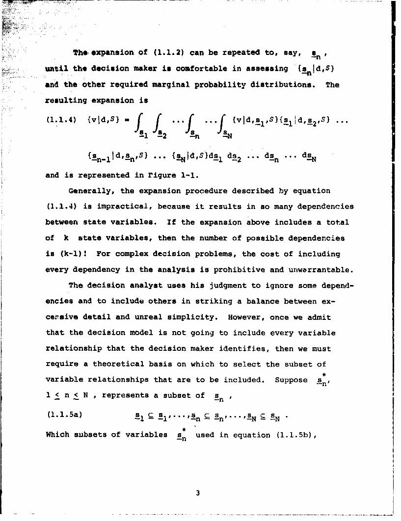
make the selection of the stochastic variables ambiguous. For

example, consider a decision model with two independent, un-

certain state variables x and x2 . Suppose the variables

have identical marginal probability distributions and different

deterministic sensitivities shown in Figure 1-2. If the measure

of the importance of a variable to the decision model is its

affect on the expectation of the profit lottery, then it is

5

.~2 2

fz f

S-1 f. f..2

x 1x 2

xi 2

VI x) I2 x

x1 x 2

FTGURE 1-2 Deterministic Sensitivity For Two Variables

6

better to fix X2 at its mean and allow x1 to be represented

as uncertain than vice versa. Because of the linearity of i,,u

deterMinistic sensitivity# uncertainty about x2 affects the

expectation of the profit lottery in the same way as it affects

the expectation of x 2 .Hence, only the expectation of x2is

required to taodel the expectation o.J the profit lottery. An-

alytical support for these contentions is provided in Chapter 3.

Two early articles by Matheson (8] and Smallwood [16] demon-

strate that one could use decision analysis to decide among

possible decision models. This approach, however, requires the

assignment of a prior probability distribution over either the

possible profit lotteries resulting from a complete analysis

(M~atheson) or the space of possible models (Smallwood). While

these studies provide an interesting conceptual tool for under-

standing the structure of a decision problem, they have not been

widely used in practice, probably because of the analyst's reluc-

tance to assign the required priors.

More recently Tani [18] suggested a variation of Matheson's

approach that can be used to quantify the dissatisfaction with a

current model. Rather than encoding a prior over possible profit

lotteries, Tani uses the differences between the current lottery

and an "authentic" lottcery, which is still a difficult assessment.

Tani assumes t.hat the marginal probability distribution encoded

on state variables are authentic.

With respect to this dissertation, Tani' s most important

contribution is the establishment of a philosophical criterion by

which to judge the "goodness" of a model. He introduces the

7

7Ft

concept of authenticity as the metric for decision models.

"Our ideal in decision analysis is not to constructthe perfect model, but rather to obtain the authenticprofit lottery -- the one that accurately expressescur uncertainty about the future." [181

An authentic profit lottery is one that accurately and fully

expresses the decision maker's beliefs. We have shown elsewhere

how an otherwise attractive structuring device is unacceptable,

because it is not related to the authenticity of the profit

lottery. (131

1.2 Practical Considerations in Structure Assessment

Three important difficulties oppose our attempts to structure

a decision problem: unfamiliarity, complexity, and numerous par-

ticipants. First, by unfamiliarity we mean the analyst's unfamil-

iarity with the political, technical, and economic influences in

a particular decision problem. The decision analysis profession

emerged from the theory with the conviction that the logical

methodology is equally applicable to all decision problems from

deciding on new business ventures or enacting legislation to

buying a house. In fact, it is the decision analyst's initial

unfamiliarity with the important relationships of the problem

that helps him to maintain the vitally important professional

detachment.. (3] However, because of this unfamiliarity, the

analyst requires tools through which the decision maker can

communicate clearly his perception of the problem structure.

A second difficulty in structuring is the complexity of the

decision problem. As the number of variables in the decision

problem increases, the structuring task becomes more difficult for

8

t~~reasons. First the number of possible relationships between

C variables increases an (n'-1)!, leading to a corresponding in-

crease in the effort rwqpried for the assessment. Secondly, the

decision maker will not apprehend some of the actual variable

relationships, because prior to the decision analysis methodology

he had no orderly way to address them. By contrast* in a small

decision problem, with few variables, the decision maker is aware

of all, the relationships between variables and has often spent

considerable time in analyzing them.

If the decision problem is complex, then there are likely to

be many participants in structuring the problem. Even when there

is a single decision maker, many experts are likely to be con-

suldted regarding the relationships between variables, as well as,

for probability assessment. Moreover; several decision analysts

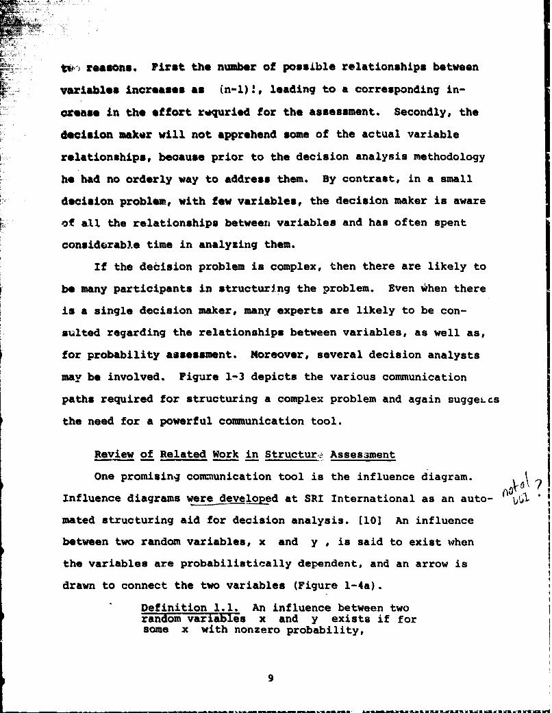
may be involved. Figure 1-3 depicts the various communication

paths required for structuring a complex problem and again suggeLCS

the need for a powerful communication tool.

Review of Related Work in Structur,.ý Assessment

One promising commnunication tool is the influence diagram.

Influence diagrams were developed at SRI International as an auto- ~

mated structuring aid for decision analysis. [10] An influence

between two random variables, x and y , is said to exist when

the variables are probabilistically dependent, and an arrow is

drawn to connect the two variables (Figure 1-4a).

Definition 1.1. An influence between tworandom variables x and y exists if forsome x with nonzero probability,

9--~-~-~----

DECISION

EXPMT DI DECISIONANALYST

DECISIONANALYST

FIGURE 1-3. Communication Paths Required For Structuring AComplex Decision Problem

10

M UffM&t UMM.&M M L f&AlA,~

F .

b:!.:

ix .C. {x,y~zjs) -" •jy, z,S}(:ly,SVIyIS}

d. {x,y,z IS) -"n bIz,y,s~{IS•Is)•s

FIGURE Iv4. The Correspondence Between Influence DiagramsAnd Assertions Of Probablistic Independence

11

WN-

(yjxs) P fyIs)

Using ihis definition, some rules for the manipulation of

influence diagrams can be derived and are discussed in reference

[10). Each influence diagram corresponds to a particular expan-

sion of a joint distribution. For example, the influence diagram

of 1-4b represents the expansnin

{x,y,zjs) - (zjx,y,s)(ylx,s){xIS.

An al.mrnative expansion, represented by l-4c, is

{x,y,z]s) - (xly,z,s)(%jys)(yjS)

and, therefore, l-4c is an allowable rearrangement of the influences

of l-4b. Comparing l-4d with 1-4c shows that the influence between

y and z has been removed, and

{x,y,RIs) a =xiz,y,S)(zIS)(yIs.

Another important property of definition 1.1 is that it appears

to coincide with the decision maker's intuitive use of the word in-

fluence. In past applications of influence diagrams for complex

decision problems at SRI International, when a decision maker or

his expert identified the existence of an influence between vari-

ables (even though it was not mathematically defined for them as in

definition 1.1), the variables were later determined to be prob-

abilistically dependent. Furthermore, influences that were iden-

tified as being strong represented, roughly speaking, more prob-

abilistic dependence than influences that were identified as weak.

Other researchers have demonstrated similar structuring devices,

such as the interaction matrix method. (2,15] This method indicates

12

the existence or non-existence of interactions or influences in a

matrix form rather than diagra atically. Rows represent a set of

variables xi U and columns y, An influence between xj and

YJis indicated by setting the ij element of the matrix to one,

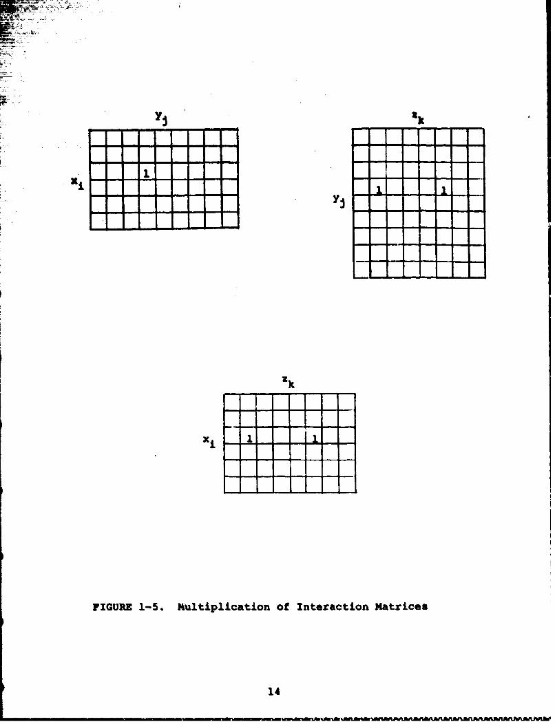
otherwise it is set to zero. When there are sequential influences,

x i influencing yj influencing ak t the matrices can be multi-

plied to show the existence of influences between x i and z k

(Figure 1-5). These interaction matrices may be quite large.

There are several important shortcomings in this approach.

First, the term "interaction" is not generally defined. It may

mean different things to the decision maker and analyst, and no

test is available to compare usage of those words. Secondly, a

ranking of interactions between x i and z k is determined by the

number of influences that exist between the two. This ranking com-

pletely ignores the questions of the degree and type of the inter-

action.

A final criticiasm of the interaction matrix also applies to

the current use of influence diagrams. Both require judgment as

to the relative importance of influences or interactions. The

analyst laments, "Everything is affected to some degree by every-

thing else," and a limitation exists on the number of influences

that can be analyzed. Since interaction is not defined in its use

with interaction matrices, we see little chance that anyone's

judgment regarding the relative importance of interactions is

meaningful. For influence diagrams, a rough notion of more or less

dependence exists, but it is not precise. Figure 1-6 shows an

example of two possible relationships of x and y In the first

13

--- _ -- ----

_ - I

z k

IIx _

FIGURE 1-5. Multiplication of Interaction Matrices

14

-A ~ Suggests a change in

{Y X,S)j

150

example the expectation of the diLEtribution on y is unchanged

Cjven the value of x .However, the variance of that distribu-

tion changes depending on the value of x .In the second example,

the expectation changes depending on the value of x , but the

variance does not. Which of the two cases represents the most

import.ant influence?

1.3 Summary and Contributions of this Research

The example of Figure 1-6 suggests that definition 1.1 is not

acomplete description of influence. While it does define theI

existence of influence, it does not describe the influence i~tself.

Most of Chapter 2 is devoted to the development of a mathematically

precise, general description of influence that is consistent with

the condition of existence given by definition 1.1. This descrip-

tion is applicable to both continuous and discrete influencing

and influenced random variables. In the final section of Chapter

2, we introduce an approximate description of influence to reduce

the informational requirement.

Section 2 of Chapter 3 shows that the influence of any vari-

able on the profit lottery can be determined by means of an in-

fluence calculus. The notation foi the influence of one variable

on another is carefully selected so that the equations for the

influence calCulus can be obtained by inspection of the influence

diagram. The implications for the decision model of the various

degrees and types of influence are conceptualized in the influence-

consequence matrix, which is presented in Section 3.4. We show how

the influence matrix can be used to estimate the differences between

16

the profit lottery from the decision model and the decision maker's

authentic profit lottery. Probably the most important philosophi-

cal result of Chapter 3 is that the selection of variables to com-

pose the decision model should depend on the decision maker's risk

attitutde. Several examples are given.

Chapter 4 compares methods for approximating the profit

lottery from information about the distribution of the profit

lottery conditioned on a state variable and the marginal distri-

bution on the state variable. First, we show that it is the

functional form of the conditional surface as a function of the

state variable that determines the amount of information required

to compute the profit lottery exactly. We also show that the

difference between the quadratic approximation, which is the basis

for the practical application of the influence concept, and con-

ventional discretization is the assumption about the shape of the

conditional surface. The quadratic method assumes this surface is

quadratic in the conditioning variable, and discretization assumes

it is piecewise linear. Since the quadratic method is shown to be

as sound theoretically as discretization and to be ccmparable in

both ease of assessment and accuracy, it should be considered ar

an alternate method for the solution of decision problems directly

from the influence diagram.

After summarizing the results of the previous chapters: Chapter

5 proposes extending the influence calculus to include decision

variables in order that the solution to decision problems can be

directly obtained from the influence diagram. We show that the

influence calculus and influence notation extend in a natural way

17

W*.. ;•' 7 i. . • •. .

to accommodate decision variables. Furthermore, the influence

vector describing the influence of the decision variable on the

profit lottery may be closely related to the solution of the

decision problem. These preliminary results lead us to encourage

further research in the application of the influence concept to

Sdeoision problems.

18

CHAPTER 2

Toward a Theory of Influence

2.1 Introduction

Influence diagrams are an attractive means for assessing

*the decision maker's structure and communicating it. However,

since only the existence of an influence has so far been

defined, the diagrams are only useful for specifying the

* existence of relationships between variables. That is, the

decision maker can indicate using influence diagrams which state

variables are members of the sets a,, *22 ~NOf the

equation (1.1.4). The influence diagram does not indicate the

nature of the conditional relationships among the state

variables, {vl.s1,d,s) or (sn-11.2n, S), and there is no

theoretical basis by which to reduce the potentially large sets

Of important state variables (expression 1.1.5).

The purpose of this chapter is to present a definition of

influence that will extend the usefulness of influence diagrams.

To that end, influence should be defined so that structuring a

decision model using the variables with greatest influence will

result in a theoretically sound decision model and lead to a

solution of the decision problem. We also want a definition

that is consistent with the intuition of both the analyst and the

decision maker . Finally practical application demands that

19

the degree of influence be either easily assessable or routinely

assessed as part of the decision analysis procedure.

Some possible definitions of influence do not result in a

useful structuring methodology for decision analysis, because they

do not focus on the authenticity of the profit lottery. For example,

mutual information is a concept from information theory that is

used to measure the dependence of two random variables. The mutual

information for variables x and y denoted by Ixly is given by

I, xyf fxyIS} log dx dy

Constructing a decision model on the basis of a variable's mutual

information with other model variables does not result in a satis-

factory decision model. (13] The reason is that muali-A rmation

indicates the importance of a variable to the system model rather

than its importance to the profit lottery. This conclusion is

congruous with Tani's claim that the purpose of modeling in deci-

sion analysis is the attainment of the decision maker's authentic

profit lottery.

2.2 Continuous Random Variables Influencing Either ContinuousRandom Variables or Discrete Random Variables

Since this section is rather lengthy and includes several

theorems, lemmas, and their proofs, Table 2-1 outlines the essen-

tial argument presented in this section. Our interest is mainlyd{yls}in the matrix d{x4S}. However, to explain the meaning of the

elements of this matrix and to introduce the notation for deriva--

tives of moments of probability distributions, it is necessary to

20

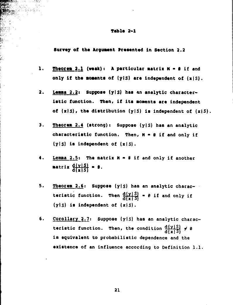
Table 2-1

Survey of the kcgument Presented in Section 2.2

1. Theorem 2.1 (weak)s A particular matrix N a I if and

only If the moments of {y}S) are independent of (xiS).

2. Lema 2.2: Suppose (yj$) has an analytic character-

istic function. Then, if its moments are independent

of (x$S), the distribution {yIS) is independent of {xIS}.

3. Theorem 2.4 (strong): Suppose (yIS) has an analytic

characteristic function. Then, N 0 if and only if

({YS) is independent of {xiS).

4. Lemma 2.5: The matrix N - 0 if and only if another

matrix r.IaI . 0.

5. Theorem 2.6: Suppose {YIs) has an analytic charac-

teristic function. Then d- 0 if and only if

{ylS) is independent of (xlS).

6. Corollary 2.7: Suppose {yJS) has an analytic charac-

teristic function. Then, the condition d xI$} 3 0

is equivalent to probabilistic dependence and the

existence of an influence according to Definition 1.1.

21

4-

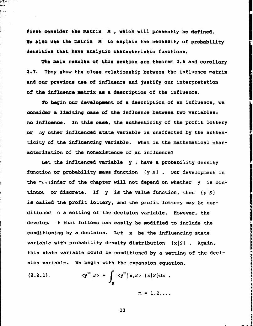
first consider the matrix M , which will presently be defined.

We also use the matrix M to explain the necessity of probability

densities that have analytic characteristic functions.

The main results of this section are theorem 2.6 and corollary

2.7. They show the close relationship between the influence matrix

and our previous use of influence and justify our interpretation

of the influence matrix as a description of the influence.

To begin our development of a description of an influence, we

consider a limiting case of the influence between two variables:

no influence. In this case, the authenticity of the profit lottery

or ny other influenced state variable is unaffected by the authen-

ticity of the influencing variable. What is the mathematical char-

acterization of the nonexistence of an influence?

Let the influenced variable y , have a probability density

function or probability mass function {yjsl . Our development in

the -.cýiinder of the chapter will not depend on whether y is con-

tinuoL or discrete. If y is the value function, then {yls}

is called the profit lottery, and the profit lottery may be con-

ditioned n a setting of the decision variable. However, the

develop.- t that follows can easily be modified to include the

conditioning by a decision. Let x be the influencing state

variable with probability density distribution {xlS} . Again,

this state variable could be conditioned by a setting of the deci-

sion variable. We begin with the expansion equation,

(2.2.1). <ymls> =f <ymlx,s> {xISldx

Vx

22 = 1,2,...

22

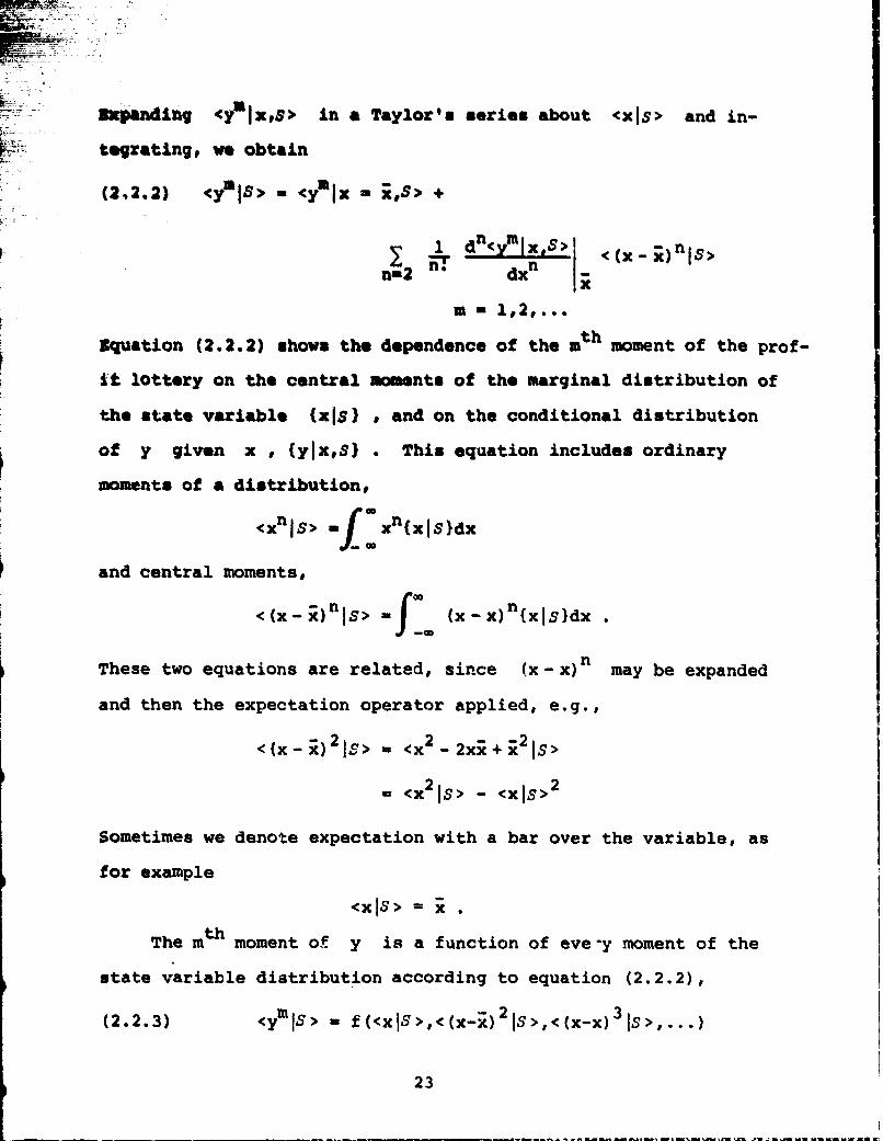
Expandinig <ylx.8> in a Taylor's series about <xls> and in-

tegrating, we obtain

(2.2.2) <yIS> - <yIx - s> +

1 d.n<yl M xS> < (X- T)nls>

n=n2 dx n

Equation (2.2.2) shows the dependence of the mth moment of the prof-

"it lottery on the central moments of the marginal distribution of

the state variable (xIS) , and on the conditional distribution

of y given x , {FyxS} . This equation includes ordinary

moments of a distribution#

<xnls> -f xn{xIS)dx

and central moments,

f -G<(X--nS -L (-)~xsd

These two equations are related, since (x- x)n may be expanded

and then the expectation operator applied, e.g.,

IS> - <x2

= <x2 1s> - <xis>2

Sometimes we denote expectation with a bar over the variable, as

for example

<xIS> = .

The mth moment of y is a function of eve-y moment of the

state variable distribution according to equation (2.2.2),

(2.2.3) <ymIs> - f(<xiS>,<(x-) 2IS>,<(x-x)3 IS>,...)

23

The functional form of f(*) is determined by the functional

r form of the conditional distributions <y xeS>. If the mth

moment of the profit lottery in unaffected by a small perturbation

in the nth central moment (n - 2,3,...) of the state variable dis-

tribution, then it must be true that

a< x-q)n < (x.i)nj S>,0<(-ns>,<x I)2s>,... n , 2,3,...

Differentiating (2.2.2) givenav^lS > I d <YPl'S>I

(2.2.4) - I n a

Ix nx"n 2,3,..,

Similarly, a< S> dy1xS dn <• Mx's> < (x-)n>(2.25) XC` 1 - M-1. -- ( Y _)n IS>(2.2.5) > dx - n-2 n d

S0 .

Both (2.2.4) and (2.2.5) are functions of the expectation of the

marginal distribution of x and both are evaluated at the nominal

value <xlS> . Equation (2.2.4) shows that the rate of change of

the mth moment of the profit lottery is independent of the magni-

tude of the nth central moment of the state variable <(x-x)n js> ,

n - 2,3,... However, from (2.2.5) the rate of change of the mth

moment with respect to <xlS> may depend on the magnitude of every

moment of the state variable distribution.

Now, suppose that the marginal distribution of the state vari-

able x is changed in such a way as to perturb its mean and central

moments slightly. If the profit lottery is unaffected by the change,

then equations (2.2.4) and (2.2.5) must hold for

24

in matrix to=i this condition is X 0 where,<%TS

.... x s

•-.-X

(2.2.6) M " •_ _

8< a<fS-; I' 9c " I > ..3cx- IS)X 9x-SIS

The authenticity of the profit lottery can only be affected

by the authenticity of a state variable distribution when the

profit lottery is altered as a result of changes in the state

variable distribution. Hence, the development of the last few

pages suggest.s the following:

Theorem 2.1 (Weak Form). The moments (if they exist) of

the marginal distribution (yIS) of a variable y are

independent of the marginal density distribution (xIS}

of a variable x if and only if M - 0 , where M is

defined by equation (2.2.6).

Proof: First, assume M- 0 . Then, by (2.2.6),

(2.2.7) 1 dn<ymIxS>1 - 0 for all m and n > 1(2.2.n T. dx' j

Hence6, <ymlx,S> is not a function of x , <yml••>- <yA'ls>

and the moments of fylS) are independent of (xjS) . Next,

25

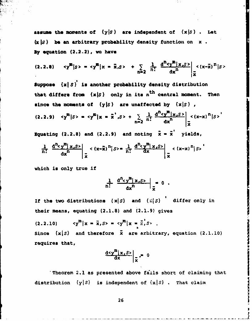
assume the moments of {yiS) are independent of (xIS) . Let

(xis) be an arbitrary probability density function on x

By equation (2.2,2), we have

1 dnCyUIx.s) > n

(2.2.8) •yls> - <r'lx- ;,s> + 1 d. <(x-x) ls>n=2 n dx n

Ix

Suppose (xiS) is another probability density distribution

that differs from NxIS) only in its nth central moment. Then

since the moments of {yis) are unaffected by NxIS} i

1d (YmIx~s> (XniS>l(2.2.9) <?m Is> M (ymjx - x ,t$ + n-19 d <(-x

n- -. d

Equating (2.2.8) and (2.2.9) and noting x - x yields,

1 n ?~y~I x,S> 1j dn<e ,>ns

n dx n I ! d

which is only true if

1 dn(ymIx~S> 0EF -d xn R

If the two distributions (xiS) and (X'IS) differ only in

their means, equating (2.1.8) and (2.1.9) gives

(2.2.10) < 7mix - ;,S> - <yjx - l,S,

Since NxIS) and therefore x are arbitrary, equation (2.1.10)

requires that,

d<ymrx,5s>d 0

"Theorem 2.1 as presented above fills short of claiming that

distribution fyis) is independent of (xIs) • That claim

26

N

requires that independence of all of the moments implies in-

dependence of the distribution itself. Under certain conditions

on {ylS) , one can show that this independence implication

holds, and these conditions lead to a stronger version of Theorem

2.1.

Lemma 2.2: Suppose {fiS) has a characteristic function

f(is) that is analytic in a neighborhood of s - 0 , where

s is a complex variable. If

<ynl$> <ynlx,$> n - 1,2,...

then

(Yls - (ylx,s)

Our proof depends on a theorem proven by Neuts [121

and restated here.

Theorem 2.3 [Neuts]. If the distribution fylS} has a

characteristic function f y(is) that is analytic in a

neighborhood of s - 0, then

M22Ii <Ykklx S> k(2.2.11) fy(is) I k (is)k=0

Proof of Lemma 2.2:

Using the hypothesis of this lemma with equation (2.2.11)

we obtain,

(2.2.12) f(is) k=0<ykx'S> (is)kk

The right-hand side of (2.2.12) is the Maclauren's series for

the characteristic function of {ylx,S} , f (.). Hence

f y(is) - fyx(is)

27

Since the characteristic function has a unique inverse,

(yIS) - (yix.s) .

While our leama is concerned only with independence, Theorem 2.3

addresses the broader issue of when a distribution is determined

by its moments. A distribution is not generally determined by

its moments, and there are several examples that demonstrate

the indeterminancyA[till ; J these same examples N prohibit

us from claiming in Theorem 2.1 that the distribution (yjs) is

independent when N - 0 . However, with the aid of Lemmua 2.2,

we introduce another theorem.

Theorem 2.4. (strong form). Suppose (yIs) has a

characteristic function f(is) that is analytic in a

neighborhood of s - 0 . The marginal distribution

(yIS) on a variable y is independent of the marginal

density distribution (xiS) on a variable x if and

only if M 0.

Proof:

First assume M - 0 . By Theorem 2.1 the moments of fyis)

are independent of {xIS) . By Lemma 2.2 (yIS) - (yIx,$s .

Next assume {yjS) is independent of NxIS) . Then the moments

of fyIS) are independent of (xiS) . According to Theorem 2.1,

M - 0 .

We defer discussion of the importance of the matrix M and its

connection with influence since there is a more useful form of

Theorem 2.4. By writing

28

/r(2.2.13) c(Y-;) mls> <?IYms> + .. + (_l)rI ?-r S> 4 Cy S>r

m -2,3*...

~K K. and differentiating we obtain,0 r m

(2.2.14) + (_,)rkmr, <YIS>r 3<ymrlS> + r<y I-rs>((M-r) <(X-i) rls>-

<Yix-r1 D~y s> J + +. 4<l~- B<YIS>

x

M = 2,p3,...n =2,3, ...

o <r <m

Each of these terms can be evaluated with the help of (2.2.4)

Now consider a matrix denoted by ýIyLIand defined by

(2.2.15) -

a< M C .

a<yS ___ ___ ___ I >X-) ,

WI29

Lemma 2.5. The matrix M -0 if and only if the matrix

&:0xS , where M is defined by equation (2.2.6) and

by (2.2.15).

Proof: For convenience of notation let N =

Suppose Mm% ,then we must show that NM =0 for

all n,m . By equation (2.2.14)

d<.y]~mS> " d<. uS> + ... + r(- m) rd< mrl>

(2.2.16) + r rI y + ...r (r+ ¶m- d<yXS>

m-r -r-l IS>+ y r y+ + r dy>

where d<.iS> represents d<(x-x)n s> for n = 2,3,...th d< (y- )Ims>

Since the mth column of N , d is a linear

combination of the columns of M according to (2.2.16),

M 0 implies N= .

Now, suppose N - 0 . We show by induction that M -

Comparing equations (2.2.6) and (2.2.15),

Mn,l = Nn,1 all n

Let

Mn,j = Nn,j j < m.

By hypothesis,

(2.2.17) M = 0 j < m.

30

Since Nnm - 0 for all n, equation (2.2.16) becomes

.(2.2.18) 0 d u S> + ... + (_1 )r (m) r d m-.is>

+ ym-r r-r-I d<yls> mim-1 d<vIy<. Is>

However, by (2.2.17)

JIS> "0 j < m,

and (2.2.18) reduces to

0 d<ym IS>0 <- iT>

Consequently

M -o 0 j <m.

By induction, N = 0 implies M = 0

using Lemma 2.5 with Theorem 2.4, we immediately obtain:

Theorem 2.6. Suppose YlyS) has a characteristic

function f(is) that is analytic in a neighborhood

of s = 0 . The marginal distribution (ylS} of a

variable y is independent of the marginal density

distribution (xis) of a variable x , if and onlyifd{yls)d{ )if -xS 0 , where dTyLS} is defined by (2.2.15).

When an influence exists between two variables, a matrix

of the form of d~x• characterizes the influence. It is a

particular representation of how the authenticity of one dis-

tribution depends on the authenticity of another distribution.

31

The nm element (n > 1, m > 1) is the effect on the mth

central moment of the influenced distribution of a unit change

in the nth central moment of the influencing distribution

(Equation 2.2.14).

Since the matrix is null when no influence exists and

indicates the type of dependency when an influence does exist,

we call that matrix the "influence matrix" or simply the

"influence" of {xiS) on (ylS} . We denote the influenced~ylS)

matrix describing the influence by d~x[S"

Many distributions of practical interest, such as the

uniform, exponential and normal, do have analytic character-

istic functions. However, it is not really necessary that the

marginal distribution {yjS) have an analytic characteristic

function. By using Lemma 2.5 with Theorem 2.1, a weak version

of 2.6 can be obtained that gives d = 0 if and only if

the moments of {yjs} are independent of (xIS) . In all the

work that follows we are only concerned with the moments of the

influenced distribution. Furthermore, wp use the influence

matrix to describe influences when they are known to exist, not

to discern their existence.

One implication of the matrix definition of influence is

that an influence diagram should be drawn as in 2-la rather than

2-lb. An influence is the impact of one marginal distribution

on another. Looking back to definition 1.1, it is clear that

the existence of an influence means that the distribution is

influenced rather than the variable. However, dafinition 1.1

is ambiguous about what the influencing factor is.

32

a.,

b.

FIGURE 21. A Comparison Of Our Representation Of Influ-ence With The Conventional Representation

33

While the difference between 2-la and 2-lb is not essen-

tial, it distinguishes influence diagrams from other structuring

devices. By emphasizing that an influence relates two prob-

ability distributions, the users of the diagrams are reminded

that the relationship may be probabilistic as well as deter-

ministic and noncausal as well as causal.

Influence Matrix Notation is Conducive toAn Influence Calculus

The notation for the influence matrix dtylst was selected

because it leads to a framework for conceptualizing and analyzing

the influences represented by a complex influence diagram. In

particular, it supports a calculus of influences.

Suppose three variables x, y, and z are related as

shown by the influence diagram below:

{xlsJ fyls) fzls}

FIGURE 2-2. An Influence Diagram SuggestingAn Influence Calculus

Given the influence of {xlS} on fyIS) , as described by the

matrix , and the influence of {yjs) on {zls} , described

by d 'YiS,, how can the influence of fxlS} on (zls} be com-

puted? Recalling Equation (2.2.3)

34

(2.2.3) <YmIS> f(<xjS> <(X-) 2 >, ... , )

every moment of (yIS) depends on every central moment of

(xIS) and its expectation. By equation (2.2.13), every central

moment of fyIS) must also depend on every central moment and

the expectation of (xIS)

%2.2.19) <(y-Yms> eM(<xls> ,'<(x-;) Is>, ..

Similarly,

(2.2.20) <:1S> - gl(<yls> ,<(y-j) 2 1S>, ... )

<(z-i9s> - gr(<yIS> ,<y-i) 2 Is> ... )

By the chain rule of differential calculus,

(2.2.21) <(-)rs> - a<(z-z)r s> > + 2<(z-i)rlS> a<(Y-)2S>a<(x-;)nIS> a<yIs> a<(x-)0nIS> a<(y-j)21S> a< (x-x)IS>

+ ..

Since (2.2.21) is the matrix product of the rth column of dfylS}

and the nth row of d ~yIS} we can write

(2.2.22) d{x S) = d{xyS{} d{yS}

which is analogous to the chain rule of differential calculus.

We pursue the calculus of influences and its form for complex

influence diagrams more thoroughly in a later section.

2.3 Discrete Random Variables Influencing Either

Continuous or Discrete Random Variables

There are many discrete events, such as whether or not it

rains tomorrow and the number of senators voting for a particular

treaty. Sometimes the probability mass function for these discrete

35

events influences a probability density function of a continuous

random variable or a probability mass function. To extend the

influence matrix concept to include this situation, let NxIS)

be the influencing probability mass function, and let fylS) be

either a probability mass function or a probability density func-

tion. The quantity x takes on the values xk for 1 < k < K

with probability PX(Xk). Our approach is to fit a continuous

curve through the points <ymjxk,S> at each point xk . Then,

these curves can be used to derive equations for <ymS> in the

same way as in the previous section. Let the function fm(x)

satisfy the following conditions:

(2.3.1) fm(xk) - <ymlxkS> k - 1,2,...

The functi4 on fm(x) is not unique, and such a function always

exists. •?or example, polynomials of degree greater than K- 1

can be found which satisfy (2.3.1). Writing the Taylor'.- series

for fm(x) about x = x gives=. f• ~1 fm-( (-x)

(2.3.2) ! r(x) f m(R) + f (.)(x-x)

n= -1

where fm= dn f m(x)n dxn

This expression leads to,

- I, xkS> Px(Xk)

(2.3.3) = [fm(m) + 1 . )nnk nni. n k x k

1 nm-'(X) + fi f n(x) < (x--£)nis>

n=2

36

Equation (2.3.3) allows us to define the elements of the

influence matrix for a discrete influencing variable with equa-

tions similar to those we use when the influencing variable is

continuous* In particular, we can write

(2.3.4) M - = (a)

III na<yms ( i nlS>

(2.3.5) f<j s> 2+ f m xW <(x-R)nIS>

and

a<(y-y) IS> I a<ymIs> +(2(x3n.S> +a<r(x-i)n) r

< (x-)S, <Is<yI~rl ~ +...+ my~smrl > m-r~~~

m=2,3, ... m

n=2,3,...

Equations (2.3.4) and (2.3.5) differ from (2.2.4) and (2.2.5)

only in the replacement of the conditional moment <ymix,S> by

the function fmo(X). Equation (2.3.6) is identical to (2.2.14).

The similarity of these sets of equations means that the

theorems and corollaries presented earlier for the case of a

continuous influencing var~ible are applicable to the case of

the discrete influencing variable. No essential changes are

required in the proofs. Hence, the influence matrix d~yS

with its elements appropriately defined, can describe the

37

a . . . . . . . . .. .. . . . .. .. . . . . . . . .. .. . .. .... . .. . . . .. .. .. . . . . . ..

iafluenoe of one random variable on another, whether the

variables are continuous or discrete.

2.4 Mpproximation to Obtain Finite Influence Matrices

On~e difficulty with the influence matrices presented so

far is that they require specifying an infinite number of

elements. To obtain the information necessary to compute the

elements, the decision analyst would need to assess the marginal

distribution on the influencing state variable and the entire

conditional surface. Table 2-2 shows that all of the moments

of the state variable distribution are required. Obtaining

all of the derivatives of the conditional surface practically

necessitates assessing the entire conditional surface. The

moments or probability densities of the influenced variablc

are also required, but in Chapter 4 we show how to obtain

these moments from other information.

Since our intention is to use the influence matrix to

structure the decision problem, an approximation to the in-

fluence matrix may be sufficient and desirable. The analysis

of the influence matrices is likely to show that some state

variables are unimportant to the problem. If a variable is

determined to be unimportant, then most or all of the informa-

tion obtained about the unimportant variable will be irrelevant

to the remainder of the decision analysis. Hence, it is im-

portant to determine the structure of the decision problem

with as little information as possible.

The numbers of nonzero elements of the influence matrix

can be reduced to four by making the following approximations:

38

31

Table 2-2

Information required to specify the Complete Influence

Matrix.

e All derivatives of every conditional moment,

dnCYm1IXS> IM 12,.dxn 1,2,...

* All moments of the state variable distribution.

<xlS> , <(x-x)lIS> n 2,3,...

39

S.. .. _

1). The profit lottery can be adequately described by

its mean and variance.

2). E'very conditional expectation and second moment

is quadratic in the conditioning variable.

The severity of the first approximation depends on the

intended use of the profit lottery. With only the mean and

variance, one can adequately represent the mean and the dis- Iperuion about the mean. In many instances the certain equiva-

lent can be determined to within a few percent using the approxi-

mation, [14]

(2.4.1) 'yls> - <yls - ½yV yIS>

This equation states that the amount the decision maker

would accept for certain, rather than face the uncertainty of

the profit lottery, is approximately equal to the expectation

of the profit lottery less an amount proportional to the variance

of the lottery. The constant of proportionality y is a measure

of the decision maker's attitude toward risk, and it is called

his risk attitude. Questions about the cumulative probability,

which are sometimes important, however, can only be crudely

answered using these approximations.

By the first approximation, the influence matrix of Figure

2-3a simplifies to a matrix with only two nonzero columns (Figure

2-3b). Approximation 2 is not an approximation of a probability

distribution by a quadratic function. Rather, it is the approxi-

mation of two functions of the conditioning variable by two

different quadratic functions,

40

-(uU) b tb- *5

a. CRIS#) •~l ,=s, I •l

ISS),Y],) I tL')l•- 1 • • •

b. ;(xjS) 8K L 2x I-S.l x

S'(x i) I(I; 4(X ) 21C. ((X4) j i s ad (Z-S) 2 Is, o

d~~xls4) a(zlSYl a l s b

0 .0

afyIS) D<ls), I Y- 2;1.=S. SC oY9 3

c o d (x Is ) 3~ lS l CXi . X IS 1, ; CX IS > ý.

I., (X-;) Is> I a- (X-g) i, s> Ij i(x--x) IIs X.

0 00

FIGURE 2-3. The Effects Of Approximations On The InfluenceMatrix

41

(2.4.2) kYo,$ + k I(x-x) + k2x-2) a 1,2

FE'-

Using only this approximation, the influence matrix of 2-3a

. s implifies to the matrix with zero elements as shown in Figure

2-3c. Applying both approximations gives the four elemuent matrix

of Figure 2-4.

Approximating the influence matrix with a 2 x 2 matrix

considerably reduces the informational requirement. The approxi-

mate matrix only requires four derivatives that describe the

conditional surface, and the mean of the state variable distribu-

tion.

42

fctS1

#i~~s -d.<YIS>Id~yS

dtCjS} dcxjS>1 d <xKl

d. < y S>tdcxS 3

- hXs~2cy < IS>hR

=k hc -2<yS>dx -

.5dxX -<

~X

wbe e * d< y 'lx,S> h1 x d2< y x sdx -dx I

hx 2

FIGUREl 2-4. The Elements Of The Approximate InfluenceIMatrix For The Influence of {xlS) on {yISl

~ w -~~~~u MJI' ~ ra'~v~~x M.E~*~ V~x ~I~WV'.1'W.43.r. n.

L... CHAPTER 3

Developing Decision Models from Influence Matrices

3.1 Introduction

The influence matrix, as developed in Chapter 2, provides

*a new way to conceptualize the influence of a variable's proba-

bility distribution on the profit lottery. In this chapter, we

show how this conceptualization can be used in the development

of a decision model. Though judgment still remains an essential

part of the decision model, intuition about the importance of

influences in the model is not required.

3.2 Influence Calculus

Chapter 2 demonstrates that an influence calculus exists for

general influence matrices. The simple example of {xIS} influencing

{yIS1 influencing {zISl suggests that the influence calculus

could be used to reduce complicated influence diagrams to simple

diagrams involving only a few variables. This simplification

would allow one to describe the total influence of any variable

in the diagram on the profit lottery.

These possibilities motivate the more thorough development

of the influence calculus presented in this section. We begin

bydemonstrating a general procedure for computing the total in-

fl uence of a variable on any other variable appearing in the

influence diagram. The total influence is the sum of its direct

44

influence on the variable and its indirect influences, through

intecmediate variables. Next, we derive the mathematical forms

for the elements of the influence matrices for several basic in-

fluence diagrams.

In the computation of the elements of the influence matrices,

we sacrifice the generality of the infinite, exact influence

matrix for the reduced complexity of the 2 x 2 approximate

matrix, though a more general and more complicated development

is possible. The influence calculus is derived for influencing

variables that are continuous. However, it is also applicable

for discrete random variables and mixtures of discrete and con-

tinuous random variables.

An Influence Evaluation ProcedureIf each of the arrows of an influence diagram is labeled

with the proper influence matrix, then the equation for the total

influence of one variable on another can be easily determined

directly from the diagram. The rule for labeling influences is

very simple. An influence is labeled as a partial influence,

for example if the influenced state variable is in-

fluenced by more than one state variable. If it is influenced

by only one other state variable, then it is labeled as a totaldfylS} Tal -1 presents and

influence, for example S Table 3-

illustrates a procedure for determining the total influence equa-

tion that uses the influence diagram and is applicable to com-

plicated diagrams. The results of the procedure for several

complex diagrams are shown in Figure 3-1.

45

v~ ~Ut~~ ~ RN'L~d~ ~~Al u K

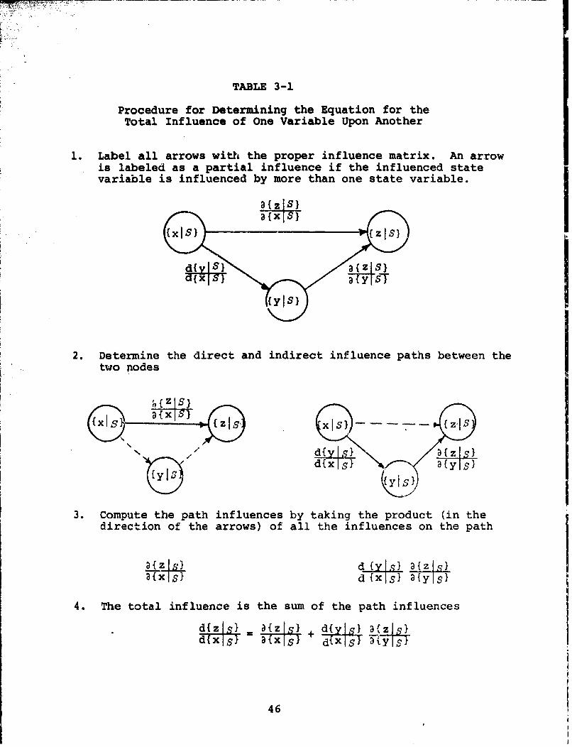
TABLE 3-1

Procedure for Determining the Equation for theTotal Influence of One Variable Upon Another

1. Label all arrows with the proper influence matrix. An arrowis labeled as a partial influence if the influenced statevariable is influenced by more than one state variable.3{zISI

2. Determine the direct and indirect influence paths between the

daxlxls3{y.s.{yXs

3. Compute the path influences by taking the product (in the

direction of the arrows) of all the influences on the path

h{zI d Y }{z Is

d~xIs} d {s}{Y S}

~{xS d{}x a{y I

4. The total influence is the sum of the path influences

d~xls} xls+ d{Xs 2y-4

46

d(zI s) di- s aujl ~zs1 d~xls) d(yls} a (zisid (wls) d(w I s}'alt!s) d~wls) d(xlsl a {y~s}

-dixis) d~zis)d~wls} dbcls}

d(zS S) {Y (v}s {z (z}

dZIS) a {(vIS} a (ZlS}

d 1z IS) (WS)1 a fyls)+dxsiavja i)

ddls dxIws) a- (zxLs) dCI(s) a (XY,91 a {jSl

a sijIs) a IylS}

d{xIsi d~xlsi +a {wls! a (vlsi

FIGUP.. 3-1. Examples Of The Influence Calculus Using TheProcedure Of Table 3-1

47

The only difficulty in evaluating the influence of one

variable on another is that all of the elements of every inter-

mediate influence matrix must be assessed.

Expressions for those elements for several common influence

configurations are derived next.

A Direct and An Indirect Influence

Consider the problem of determining the total effect of a

change in the marginal distribution of a state variable on the

distribution of another state variable. Suppose that the in-

fluencing state variable has both a direct influence and an in-

direct influence, through another state variable. An example of

this problem is calculating the total influence of NxIS) on

(ziS} in Figure 3-2.

{x~s) yzss

FIGURE 3-2. An Influence Diagram with a Direct

and An Indirect Influence

To compute the total influence, we begin by expanding

<zlx,y,S> in a Taylor's series, multiplying by {x,yIS} , and

integrating. The result is

1 x v<,x1 > + if jS+ Coy (x, Y)(3.2.1) <zIs> = <+ fax V>x +2 yy xywhere

Sfx a <zlx's f• a> •2 < z X, xyS> ec- Xa xx etc.

x~y,4

48 i

Taking the partial derivative with respect to <xis> gives

(3.2.2) a~ + f 9 O (,Y13..a <x IS> , x fxy a<xIS> x~-

Notice that fxx F fyy . and fxy are constants by the assump-

tions made in Chapter 2. Equation (3.2.2) is the direct influence

of <xls> on <zIS> . To evaluate it, the change in the co-

variance due to a change in the mean of {xlS} must be determined.

First, we can express Cov(x,y) in terms of the moments of

{xISl , according to Appendix A,

(3.2.3) Cov(x,y) 1 ! dn<y.xS> <(x,-) n+lS>nin. dn-n=l dxn

A similar expression could be derived for terms of the form

<(X-x)n (y-y)mlS> , which would arise if terms of greater than

order two were included in equation (3.2.1). Hence, a more gen-

eral development of this type is possible.

If the conditional surfaces are approximated with a quadratic

function in the conditioning variable (approximation 2 of Chapter

2), then

(3.2.4) Cov(x,y) = hx V<xlS>+ Pxx <(x-x IS3>

where2

h = a<ylx,S> and h =Sa x xx 2

Ix ax I-

Equation (3.2.4) expresses Cov(x,y) in terms of <xls> , and

V <xlS> .However, Cov(x,y) can be written as a function of

49

<xlS> and <Yls> using(3.2.5) <yjs> . <y1js> + I hxx V<xls>

Solving (3.2.5) for V<xlS> and substituting into (3.2.4) pro-

duces,2hx

(3.2.6) Cov(x,y) Wi- (<yIS>-<y I,S>) +2 hxx <(x-i) 3 Is>xx

In this equation <xlS> and <ylS> are independent variables.

As a result, the required derivatives of Cov(xy) can be

evaluated,

h2(3.2.7) -Cvxy 2, 21<yl S>_<yI•S>) - 2

2hh2

and.7 acov(x .v) -h <S>-,S h x

xxand

x

aCov(xf•) hx(3.2.8) 8<ylS> - 2 --.

xx

Again, hx is constant by our approximations in Chapter 2.

Substituting (3.2.7) into (3.2.2) yields,

(3.2.9) <Z S> V< > 2 X•<X S> x fxy hxx hx

A similar expression for the partial derivative with respect to

<Yls> can be obtained with the help of (3.2.8),

(3.2.10) B<z S> =f + 2f h x<y S> xy hxx

50

This equation gives the direct influence of <y S> on <zIS>

The total influence of cxjS> on <zjS> can be obtained

by using (3.2.9) and (3.2.10) in

d<z S> = <zls> +d<x.5> - - -(3.2.11) d<xlS> j,• > ;,i + -,a a•<Sj> y

+ d IS> I <zzIS>a<x-7>- ,iv<,I S>I - -

Equation (3.2.11) says that the total influence of <xiS> on

<zlS> is the sum of its direct influence and its indirect in-

fluence. The factor a.<V<yls> is found from (3.2.1) to be fav<yjIs> i yy

A similar derivation leads to an expression for the influence

of V<Xls> on <zls> :

d<zIS> - - = B<zIS>> + d<yS> - <zls>dv<xjsý ,' y •V<XIS> XO, dV<x Sq>j xIy TZ_,• I~

(3.2.12)

+ aVS<S> <z Is> Id V<xls> Dv<yls>

where V<zIS> = 1 fx <yIs> 1f '

2<z xS> =hfy a x

a<y s> f +xy x

Equations (3.2.11)and (3.2.12), along with expressions for

dV<zlS> d<z21S> - 2<S> d<•-- >d<x s> dx,> - d'zx S>

51

and d<S>.d<zZs 2 IS d<zSv 2______zls __ _ _dv s

dv<xlS> dv<xlS> d <xlS>

can be combined in the convenient influence matrix form for the

total influence of (xjS} on (zisi ,

d .- d<zis> - -<x -

Ix,Yx

"a{zls} d{yIS} a{ziS)(3.2.13) =Tx. + dixISl F)yTST

The total influence is the sum of the direct influence,d{y lS} ý{--, S} Fi u e 3 3 n

and the indirect influence lS} T Figures 3-3a and

3.3b detail the elements of selected matrices of this equation.

A Special Case

A special case of two influencing variables occurs when

either of the following conditions holds:

a) Cov(x,y) = 0

b) a2<zixy> a = 2 <z2Ix'y>L = 0:y ;,s ,axay

In that case, Equation (3.2.1) reduces to

<ziS> = <zixyS> + f V<xlS> + fyy

from which we find

52

VC

3.<" s 3xIciis,

*2< z I S>fxy

(~V< Z S>-2h 2 Axy x

w b ere d < y lx 's ý-d l1 .ý S

xd

f . L<zx~ f <zxrf>-Z Ixty? S>X a x xx ax2Xt jj X 3 xa y I

~ I*a.e 2Y'y~ *a <Zlxf

X" x'ry li

FIGURE 3'3a, The Elements Of The Influence Mratrices OfEquation (3.2.13)

53

a~ ~ 8uSI

-Ca~ a L- I4' -C2& z..sIVf18

fý+2f~yh/2g /g (h -2oZssf )2gx /xxh yx -c fxy)

5f .5f y * (~ZIS>fyy

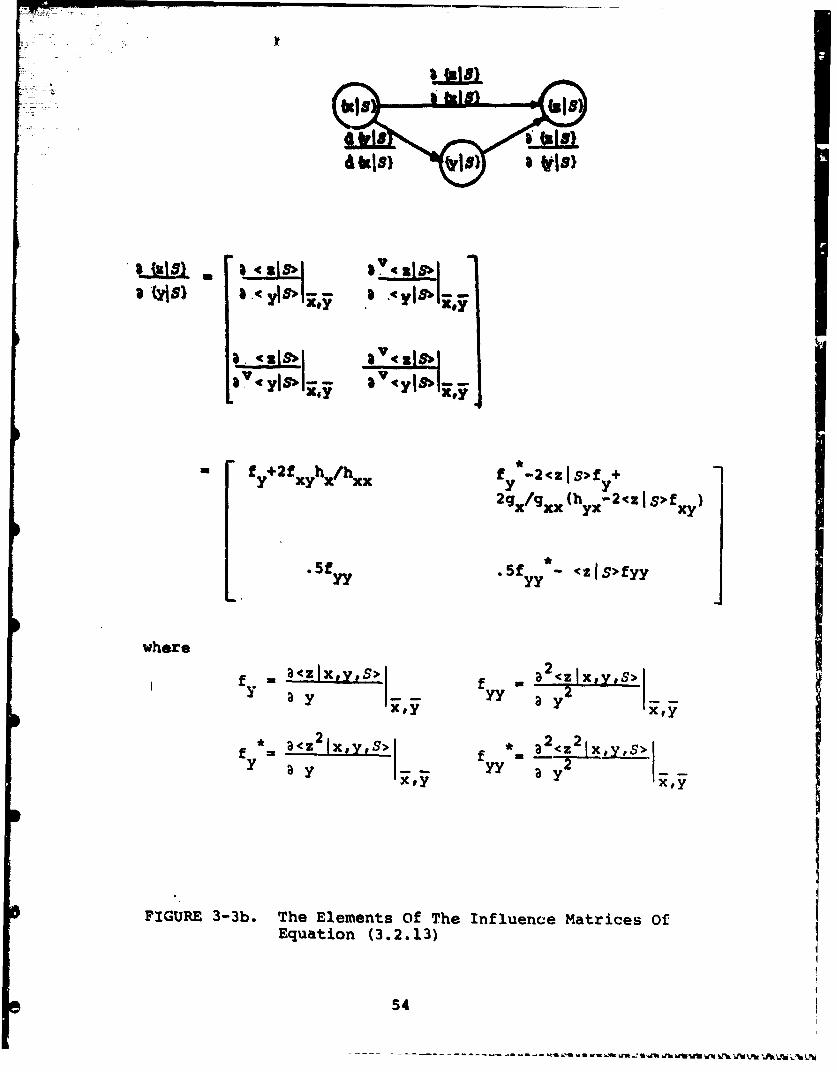
where

-y a3czIx.Y#S> <jXV

y yy a_ Y2 2xt

FIGURE 3-3b. The Elements Of The Influence Matrices OfEquation (3.2.13)

54

-------------- ~

= 8<21s), 3<zlxoY,,s>

These conditions produce a simplification in the influence

matxix, which is evident comparing as shown in Figure

3-3a with

(3.2.14) "{Ii. 1/2.f1 f * 24(ZIS~f

xx 1 2 xx - <zS>fxx

The direct influence matrix of (3.2.14) can be determined with-

out information about <ylx,S> . Furthermore, under these condi-

tions we have

fx ax •<zx' ' y

f <z Ix,S> Ix ax "I x

and similar expressions for fxx , f x , and f ." Hence, the

elements of (3.2.14) can be determined independently of the in-

fluence of {ySl}

Of course, condition a) holds for the situation depicted in

Figure 3-4. In that case there are no indirect influences,

and equation (3.2.13) simplifies to

(3.2.15) d~zlf} = a{z1S}

where a is given by (3.2.14).

55

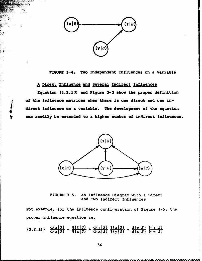
FIGURE 3-4. Two Independent Influences on a Variable

A Direct Influence and Several Indirect Influences

Equatitm (3.2.13) and Figure 3-3 shov the proper definition

of the influQnce matrices when there is one direct and one in-

direct influence on a variable. The development of the equation

can readily be extended to a higher number of indirect influences.

(ZISI

FIGURE 3-5. An Influence Diagram with a Directand Two Indirect Influences

For example, for the influence configuration of Figure 3-5, the

proper influence equation is,

(3.2.16) dix]S) W a{x SA d }x S) a{YjS1 + d{xlS} a{wls)

56

The elements of selected matrices are displayed in Figure

3-6a and 3-6b.

The covariances between each variable that influences {zIS}

and all of the other influencing state variables must be con--sidered in computing the direct influence of that variable.

Evaluation of the elements of (3.2.16) requires that assess-

ments be made of the mean and variance of z conditioned on the

three variables x,y,, and w *It can be easily extended to the

the appropriate equations can be written down by inspection of

(3.2.13) and (3.2.16). The practical limitation on the exten-

sions of (3.2.16) is the difficulty of assessing moments con-

ditioned on more than three variables.

3.3 Influence Vectors

When the influenced marginal distribution is the profit

lottery, it is sometimes unnecessary to describe the influence

on the entire distribution. Often the certain equivalent ade-

quately characterizes the profit lottery. In those instancesI

a decritio oftheinfluence on the certain equivalent may be

sufficient.

Howard [5] showed that the certain equivalent could beI

represented as a ?ower series:

= k: Z k-Ik=lk

wherey =the decision maker's risk aversion

coefficient

57

8(xS} h 2 2(hIS V 2h 2

xyIS fx~~>) +x fx IS>--i--f + 2zsfy+

(hh

2g2 2g

S> 2gx- S> Sg f

where

fx = 3 <zlwfx"y,S> f x a<z 2 jwx1yS>a 3x a 3x

a x a I

etc.

FIGURE 3-6a. The Elements Of Selacted Influence Matrices ofEquation (3.2.16)

58

{zS, f +2f X.. + fx-2<~ +

3(yj Yhxxv ~2k

khyy x

(k <.5f,-< )( S -2<f S~

where

k y etc.y

yIFIGURE 3-6b. The Elements Of Selected Influence Matrices of

Equation (3.2.16)

59

k kthz the k cumulant of the profit lottery.

By truncating the series and evaluating the cumulants, one can

obtatn an expression of the form

(3.3.1) <zjS> C c1<zs> + K C <(z-) kIS> Yk-i

Por example, with K-2 , =1 and C - If we let

(3.3.2) C - [C 1 C2Y C32 ... Ckk 0 0 0]T,

then we can define an influence vector

(3.3.3) d $ <x S> C <x 2 "2RIS [a< 1>X-x) Is> -I

According to this equation, the influence of {xlS} on the

certain equivalent of the profit lottery is described by a vector

of changes in -<zlS> resulting from changes in the expectation

and central moments of xlS}•

The influence calculus applies to influence vectors as well

as influence matrices. For example, if

d{zIS) :-d{xlS} d{yl•T '

thend -x IS>, = d{z S) CW

(3.3.4) =- S}.d<zS>

A special case of Equation (3.3.3) occurs when k= 1 in

- -- - - - - -- - - -- -- -60-

4pqquation (3.3.1), then (3.3.3) becomes

'.;i•,-d<xs I> d{z J..q [1 0 0 ]T(343.5) (i o} *

, "[~d<z IS> d<zlx-S2> T•"dC~X)ISLX

3.4 An Example Introducing the Influence Consequence Matrix

We have shown in preceding sections that the influence

matrices when combined using the influence calculus establish

how changes in the marginal probability distribution of a state

variable affect the profit lottery. Wc have also suggested

that the relative importance of these changes is measurable byd"< zlS>

the change in the certain equivalent, e.c,. " In this

section we propose a method for combining the theory of influence

with the judgment of the analyst aa an aid in developing the

diicision model.

To illustrate the method, we make use of a modified version

of the entreprenuar's decision problem, posed by Howard [5].

The entreprenuer must decide upon the price of his product P

in the face of uncertainty about demand, q(P), and the cost of

his product C(P). His profit function is

ir(C,q,P) , Pq(P) - Cq(P)

The variables C end q are assumed to be uncertain. Letting

6C = C -

Aq = q - q

allows definition of Air (AC, Aq,P) as

61

(3.4.1) AW(AC,AqP) ' P[q(P) + Aq] - C[q(P) + Aq] - AC - 7r(C,q,P)

which is the change in profit due to fluctuations of C and q

about their means. Both {AqjS) and (ACIS} have means of

zero and

v<ACIS> - 10000

V<AqlS> 100

An influence diagram for the original problem with modifica-

tions is shown in Figure 3-7. The random variables Y , E , and 6

have been added and the dependencies of the moments of

{ACIy,e,S} and {AqI6,E,S} are presented in Figure 3-8. For

example, e can be thought of as a general economic indicator.

As e increases both <ACIy,e,S> and <AqI6,c,S> are assumed

to increase linearly, but the corresponding variances do not

increase. A similar remark holds for the relationship between

AC and c . The following marginal probability densities have

been assumed:

(3.4.2) {yIS = 0 <6<101

{CIS} < C < 1

{61s1 26 0 < 6 < 1

From the original entreprenuer's problem, we find

2(3.4.3) An(0,Aq,P*) = 17.58Aq + .0249(Aq)

and

(3.4.4) An(AC,0,P*) = - AC

where P* is the optimal setting of P when AC = Aq = 0 . All

62

Boundary of original entreprenuer's problem

FIGURE 3-7. Influence For The Modified Entreprenuer's Problem

63

r4

0 S

r4

9:00 I40 (

C.W.

r4 E-4 04

P4 4

P0141)0

A.- A

old * 5 544

64 .1

of the following is conditioned on P - P,

if we assume the deciaibn maker is risk neutral, then by

(3.3.4) the influence vectors are

,<•,Pf$> [NWP'rS>I 8<wlp'"> I

3 at q j s ' = ' < A q l S > - V < A l > -

T q aip s <_ &q_ S >_ _ _

The cross-partial is3A 1 zero according to (3.4.1).

Therefore, (3.4.5) can readily be evaluated, using (3.4.3) and

(3.4.4), As

•(3.4.6)T<AwIP*S> L S> IT

I- [17.6 I2

and

a<2 <*W1> 1 T

( 3 .4 .4 ) , a scf

> ] Ta=P S> 1 0 .

The elements of the influence matrices for state variables

y,6, and e can be determined from Figure 3-8. The matricesare shown in Figure 3-9, along with the computations for thetotal influence on the profit lottery.

The influence matrices can be useful in explaining the type

and strength of relationships between state variables and the

profit lottery. Examining the influence matrices shows that

{YIS) affects only V<ACIS> , and V<ACIS> does not affect

65

d•,uS . 3-(cIS) dc,IS>

d y I S) •' 'I S) d 'Ac IS10 :i(S6 1 - FII!<,..I.s- a' rA~jI S) d C., S>

d 6 Is) a' 6IS} d'{AqIS)

- 0 356 187 17I-Loo ,2671.- -1 [26.6

dSIS>, A{^cIS) <Is + I'{Assg} Sd<,lSdrlS}) a'etlS d{AtcIS) a' S)Isl d{AqIS}

r1o0 1 [13][

0 1335 j 0 1 0 V .025]

FIGUPE 3-9. The Influence Matrices For The InfluencesOf Y,#6, and c.

66

<rjP*,•) . Consequently, neither <y7S> nor v<yIS> affect

tho expectation of the profit lottery. On the other hand,

<w1PrS> is affected by V ,AqIS> Therefore, {61SJ affects

the profit lottery even though it affects only V <AqS> . Theeffect of <61S> on <%IP*,S> is small., because it acts though

its influenoe on V<Aql$>. <cS> has a much larger effect on

<clP*,S> , because it acts though its influence on <AqlS> IThe effect of <eIS> through <AqjS> is partially cffset by an

opposing effect through <ACIS>

Selecting Variables for the Model

Sometimes the influence matrix itself will indicate that

a particular variable is unimportant to the problem and need not

be included in the model. For exanple, since <nIP*,s> is un-

affected by the distribution on {61S} in the exampie, the

decision maker will not suffer if {61S} is omitted from the

model.

In general, the analyst must use his judgment to interpretm

tbe influence matrix. Figure 3-9 shows that <n!P*,S> is more

sensitive to the mean of {eJS than to the mean of {61S}, but

is less sensitive to the variance of {cIS} than to the variance

of {61S} . Should the uncertainty of both of these variables

be included in the model, or only one? If one is to be uncertain,

which one should it be?

To clarify the roles of the influence matrices and the

analyst's judgment, we introduce the expression

d <zlS> A<x(3.4.6) I i<,s> I

67

The factor -TRN is the first te~m of the influence vector

d <f1 of equation (3.3.3).

In the context. of the influence matrix, we think of it as

the change in the certain equivalent due to a change in the mean

of NxIS) However, it may also be interpreted as the deter-

muinistic sensitivity of the certain equivalent to a unit change

in the variable x about its mean. The factor A<xIs> expresses

the decision analyst's judgment about the difference between the

mean of the distribution assigned to x and the mean of the

decision m~aker's authentic distribution on x .This differenceI

may be due to difficulties in the assessment procedure, a hasty

assessment, or the fact that the state variable is influenced by

many other variables. Therefore, the quantity given by (3.4.6)

is the change in the certain equivalent that results from ob-

taining an authentic mean of the state variable distribution.

If the value of expression (3.4.6) for a particular state

variable is a large fraction of the certain equivalent or the

difference between certain equivalents for different decision

settings, additional modeling or more careful assessment of that

state variable is warranted. If the value is small, then other '

state variables should be considered for additional work.

The number of variables that are treated as uncertain inI

a decision analysis problem is usually constrained to six or seven

due to time and budget limitations. Therefore, identifying whichI

variables should be represented as uncertain is an important

concern. While (3.4.6) can be used to indicate the importance

68

of further modeling, a similar expression indicates whether a

particular state variable should be treated as a random variable

or whether the uncertainty can be ignored and the variable fixed

at its mean value. The factor d<&IS>a in expression (3.4.7),

d'<ld V<xlS> ,

(3.4.7) v< s>dx<SzI S

is the second element of the influence vector dUR }1

We could have multiplied df<zIs> by a factor AV<xlS> ,dV<xl s>

the decision analyst's judgment about the difference between the

variance of the assigned distribtuion and the authentic distribu-

tion on x .However by multiplying by the variance v<xlS>

rather than the change in variance, Equation (3.4.7, approximates

the change in certain equivalent that results from fixing x at

its mean and not treating it as a random variable. Appendix B

gives a proof that under the approximations made earlier

(3.4.8) 3~<zls> v<xls> w-<zls> - <zlx , s> .a V<xls>

The influence-consequence matrix of Figure 3-10 conceptu- Ualizes the implications of the various combinations of magnitude

for the modeling indicators of (3.4.6) and (3.4.7). The top

portion of each matrix entry recommends an action regarding the

improvement of the authenticity of the distribution assigned to

the state variable. In the lower portion of each entry is a

69

A•_

•t

d-- 8 39 S1I

Model NoFurther FurtherModeling

Uncertain Uncertain

IdVcxt[S> c~:

Model NoFurther FurtherModeling

SMALL

Fixed At Fixed AtMean Mean

FIGURE 3-10. The Influence-Consequence Matrix

70 J

recommendation about whether that state variable should be con-

sidered as uncertain or should be fixed at its mean in the

de-'ision model.

Of particlar interest is the lower left element, which

corresponds to a large change in the certain equivalent due to

anticipated changes in the expectation of the state variable,

1)ut little change when its uncertainty is ignored. In this case,further modeliiig is recommended to more accurately determine the

mean of the state variable. A model of the influences on tie

mean of that state variable might include uncertainty, even

though -he influanced variable itself is not treated as uncertain

in the decision model. To otr knowledge, this option has not

beei exercised in decision models, ard it is a new result of our

analysis of influences.

Returning to the illustrative entreprenuer's problem, Table

3-2 shows the values of (3.4.6) and (3.4.7) for the state vari-

ablo- Y,6, and E . Since a numerical estimate of the difference

between the a.sessed mean and authentic mean is required for each

state varia,.. e, we have assumedr<xls> = .1 V<xls>

This expression reflects the feeling that the mean of a broad

distribution is less authentic than the mean of a narrow distribu- 0

tion. Of course, other functional forms might also be used.

As we mentioneJ above, y is irrelevant and may be|

ignored. mveating e as uncertain is not necessary, since its

uncertainty inly contributes .08 to the expected value of 200.5

71

Table 3-2

The Influence of the Variables y, c, and 6

and the Modeling Consequence

I.

Y' 6 £

311S> 0 8.7 76

a<ffIs>

•<rIS> 0 6.6 .25

av<. I s>

_<_ >_ .1 x F<. Is> 0 .16 4.4a<* IS>

x<jS> V< 1 S> 0 .37 .08a v<. IS>

No Further No Further Further

CONSEQUENCE Modeling Modeling Modeling

Fixed At Uncertain Fixed At

Mean Mean

72

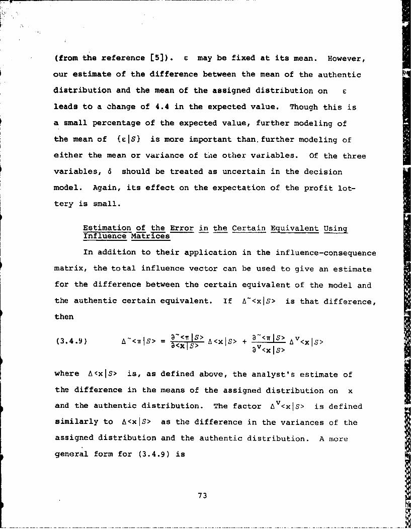
(from the reference [5]). e may be fixed at its mean. However,

our estimate of the difference between the mean of the authentic

distribution and the mean of the assigned distribution on C

leads to a change of 4.4 in the expected value. Though this is

a small percentage of the expected value, further modeling of

the mean of {jIS} is more important than further modeling of

either the mean or variance of tie other variables. Of the three

variables, 6 should be treated as uncertain in the decision

model. Again, its effect on the expectation of the profit lot-

tery is small.

Estimation of the Error in the Certain Equivalent Using

Influence Matrices-

In addition to their application in the influence-consequence

matrix, the total influence vector can be used to give an estimate

for the difference between the certain equivalent of the model and

the authentic certain equivalent. If A~<xlS> is that difference,

then~<7 IS> ___<____

(3.4.9) At<r Is> = a<x s> A<xls> + V<T Is> Av<xls>a <.Xls aV <x lS >

where A<xlS> is, as defined above, the analyst's estimate of

the difference in the means of the assigned distribution on x

and the authentic distribution. The factor A V<xIS> is defined

similarly to A<xlS> as the difference in the variances of the

assigned distribution and the authentic distribution. A moregeneral form for (3.4.9) is

73

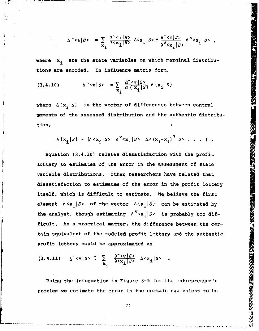
a ~<7 I S> A<X IS> + __ IS>a, a8> 1 v< A<xis> •

where xi are the state variables on which marginal distribu-

tions are encoded. In influence matrix form,

(3.4.10) A-<IT IS> d <7lS A {xi IS)•x.T T xils}1

where A{xils} is the vector of differences between central

moments of the assessed distribution and the authentic distribu-

tion,

A{xiIS} = [A<xiIS> AV<xils> A<(xi-xIS>

Equation (3.4.10) relates dissatisfaction with the profit

lottery to estimates of the error in the assessment of state

variable distributions. Other researchers have related that

dissatisfaction to estimates of the error in the profit lottery

itself, which is difficult to estimate. We believe the first

element A<xiIS> of the vector A{xilS} can be estimated by

the analyst, though estimating A V<xiJS> is probably too dif-

ficult. As a practical matter, the difference between the cer-

tain equivalent of the modeled profit lottery and the authentic

profit lottery could be approximated as

(3.4.11) A~<vlS> I a~<v1S>Xi 1 S> A<xilS>

Using the information in Figure 3-9 for the entreprenuer's

problem we estimate the error in the certain equivalent to be

74

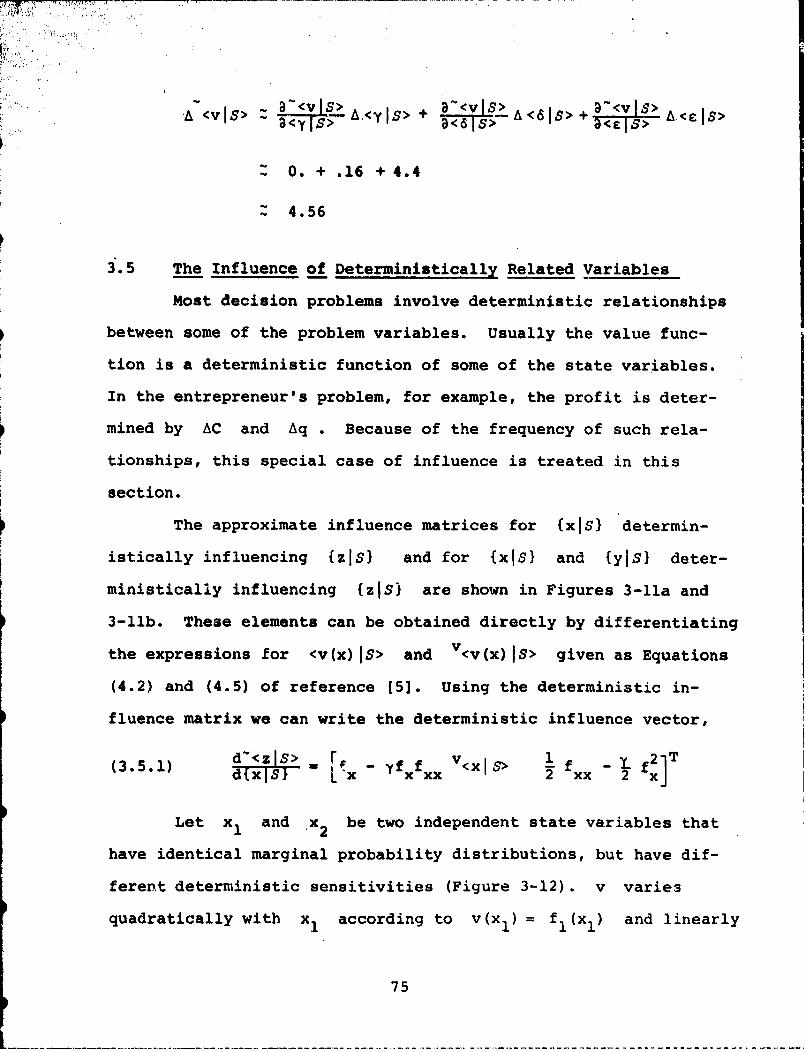
PI•A~<vIS> a L + <. Is>+s> <6Is

Z 0. + .16 + 4.4

Z 4.56

3.5 The Influence of Deterministically Related Variables

Most decision problems involve deterministic relationships

between some of the problem variables. Usually the value func-

tion is a deterministic function of some of the state variables.

In the entrepreneur's problem, for example, the profit is deter-

mined by AC and Aq . Because of the frequency of such rela-

tionships, this special case of influence is treated in this

section.

The approximate influence matrices for {xIS} determin-

istically influencing {zjSl and for {xjS} and {yjS} deter-

ministically influencing {zjS} are shown in Figures 3-11a and

3-11b. These elements can be obtained directly by differentiating

the expressions for <v(x) IS> and V<v(x) IS> given as Equations

(4.2) and (4.5) of reference [5]. Using the deterministic in-

fluence matrix we can write the deterministic influence vector,

(3.5.1) d-<xlS)> . - yf f V<2 x -f f2]Td~xTS1T LX x XX 2 xx -2 xj

Let x1 and x 2 be two independent state variables that

have identical marginal probability distributions, but have dif-

ferent deterministic sensitivities (Figure 3-12). v varies

quadratically with x1 according to v(x 1) = f 1 (x1 ) and linearly

75

a WxS) a Z S

a. -Cz S> aVzSa C ~I S> 3s a V~xI5 > it

y gv >2 9 <y19

xx y xy

2 (gxgygxy) hxV<x 194~

29g (QV4 I 3-2hx 2/h=)

.5&g f 2

weea z(x,y) g a 2 z tx~y)I .z (X,y) etc.

r dcylx,s>

xO,Y

FIGURE 3-11b. The Approximate Influence Matrix For Determin-istic Influences

77

V-f 1 (x1 ) Vf 2 (x 2 )

---- - , S ; .- - - -I

il l xi 2

II Ix 2

FT GURE 3-12. Deterministic SensitiviLy For 'wo Variables

78

with x 2 , V(x 2 )- f 2 (x 2 ). By expression (3.4.7), the change in

the certain equivalent due to fixing xI and x2 at their means

are, respectively,

(3.5.2) d<v[S> V<x Is> -f + fl2 V<xls>dV<xlIS>

(3.5.3) d'cvIS> V<x 22s, = + j f 2 v<X21s>dV<x 2 1S>

Now, suppose that the budget constraint on the analysis

is such that only one of these two variables can be included in

the model as uncertain, and the other must be fixed as its mean.

Policy regions for this decision as a function of the decision=1an

maker's risk tolerance p and f 2 can be obtained byY2

equating (3.5.2) and (3.5.3). Figure 3-13 displays the resulting

diagram.

Risk Neutral Decision Maker Is Concerned About Nonlinearity

The most surprising feature of the figure is that for risk

neutral decision makers, x1 is the variable that should be

treated as uncertair, in order to minimize the error in the cer-

tain equivalent of the profit lottery. This result is easily

seen by setting y - 0 in Equations (3.5.2) and (3.5.3). It is

surprising because tV choice between x and x 2 does not de-

pend on the slope of the deterministic sensitivity plot. Even

though the change in Uic u.L La... &....e.aL be•.%L.W-.. =... ....

values of x 2 could be greater than the change between extreme

values of xl, it is xI that should be included as uncertain.

79

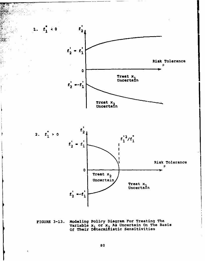
1.ff f2

Risk Tolerancep

0Treat x

" I Uncertainf2 r-fl

Treat x•Uncertain

f2

2. f: 0 f 2

22

, , f'12/flf 2 f f1

Risk Tolerancep

0 Treat x 2 Tet

Se Uncertain

f2 "-fl

FIGURE 3-13. Modeling Policy Diagram For Treating TheVariable x or x As Uncertain On The BasisOf Their Diternmihistic Sensitivities

80

The linear variations of the functions f 1(W and f 2 (x)

do not appear in the expression for <v(x) IS> . Consequently,

the risk neutral decision maker needs to concentrate only on

modeling the nonlinear dependency of the value function on the

state variable x, , because that dependency alters the expecta-

tion of the profit lottery. However, the linear variations of

the decision maker's risk tolerance decreases, ne is increasingly

concerned with the risk premium and the linear terms. The risk

averse decision maker must balance the error that is made by

ignoring the effect of f 2 (x) on the risk premium against the

errors made by ignoring the effects of f Wx and f (x) on

the risk premium and the effect of f (x) on the expectation of

the profit lottery.

De~nencyof the Decision Model on the Decision Maker's

Perhaps a more important philosophical issue suggested by

Figure 3-13 is the implication that the choice of variables for

the decision model should depend on the decision maker's riskI

attitude. Two decision makers with the same information about

aproblem but with different risk attitudes may model a decisionI

problem differently.

Decision analysts have always distinguished themselves

from other modelers by insisting that the specifications of aI

model.be determined by a particular decision. Our work suggests

that the specifications of -!le model must not only be determined

__ _ 81

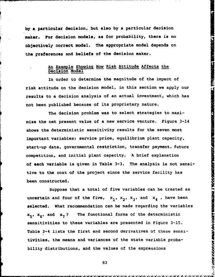
by a particular decision, but also by a particular decision

maker. For decision model., as for probability, there is no

objectively correct model. The appropriate model depends on

the preferences and beliefs of the decision maker.

An Exml Shwn How Risk Attitude Affects the

Dec i7ion Mod-el

In order to determine the magnitude of the impact of

risk attitude on the decision model, in this section we apply our

results to a decision analysis of an actual investment, which has

not been published because of its proprietary nature.

The decision problem was to select strategies to maxi-

mize the net present value of a new service venture. Figure 3-14

shows the deterministic sensitivity results for the seven most

important variables: service price, equilibrium plant capacity,

start-up date, governmental restriction, transfer payment, future

competition, and initial plant capacity. A brief explanation

of each variable is given in Table 3-3. The analysis is not sensi-

tive to the cost of the project since the service facility has

been constructed.

Suppose that a total of five variables can be treated as

uncertain and four of the five, x 1 . x2 ', x3 P and x , have been

selected. What recommendation can be made regarding the variablesI

x5,, x6, and x7 ? The functional forms of the deterministic

sensitivities to these variables are presented in Figure 3-15.

Table 3-4 lists the first and second derivatives ot these sensi-

tivities, the means and variances of the state variable proba-

bility distributions, and the values of the expressions

82

TABLE 3-3. Brief Explanation of the StateVariables in the Example Problem

x Service Price - Since this service is unique in the U.S.,a large uncertainty exists about thedemand curve.

x2Eguilibrium, - Though the plant that provides the servicePlant Capciy is constructed, it has not operated, and

new technology is involved.

x Start-up Date - Even if the owners decide to begin plant3 operation as soon as possible, the actual

start-up date is uncertain. Delayedstart-up reduces the present value of theprofit stream.

x4Governmental - Because the client is currently the onlyRestriction company able to provide this service, the

possibility of government restriction ofprofit exists.

x 5Transfer - Part of the service is performed by anotherPayment company. The cost of that service is un-

certain.

x6Future - Competitors may enter the market in theCompetition future.

X 7 Initial Plant - The plant is expected to start productionCapacity at less than equilibrium capacity. Early

capacity is uncertain, however.

84

v,net presentvalue

"590

570

x 6

-530

x7 x 5

1-510

i-a< xiIS> x + iIs>

FIGURE 3-15. Functional Forms For The Deterministic Sensi-tivities of x5,x6 and x7 .

85

r-7

A

0 > V 3%

0%%

0 A A N

04

. - - !

A

$.n44

v. 0'4

5 r40

fdIn

U) "E-4 4

'4.4 it 1

'.4 4V4 k '. 4 q

.44 *44U Na

f40 FA "q

-- _-

d-vS S> )•x S> and d-vIS> VcxivS>Id~c jAi. (. . x sd Is> i

Recall these last two expressions approximate, respectively, the

change in the certain equivalent due to a change in the mean of

a state variable and the change in the certain equivalent due

to igncring uncertainty in the state variable.

This table reveals that the variable with the largest

deterministic sensitivity x5 is not the first one that should be

treated probabilistically. To the contrary, x7 , with thesmallest sensitivity would piLoduce the greatest change in cer-

tain equivalent if its uncertainty was ignored. As we discussed,

in the previous section this effect is the result of the non-

linearity of the determinis sensitivity of x 7 , as seen in

Figure 3-15.

As we might expect, obtaining an authentic mean for vari-

able x5 is more important than for variables x 6 and x7

Upon inspection of the influence consequence m- (Figure

3-10), of the three variables x5 , x 6, and xT, x 5 and x6

should be fixed at their means, but x5 should be carefully

assessed or futher modeled.

Finally, the modeling policy diagram for the decision to

treat x 5 or x 7 as uncertain is shown in Figure 3-16.

87

10-

Treat x

UncetainUncertain

5-

f; Risk Tolerance

0

100.; 200 300

-10

FIGURE 3-16. M4odeling Policy Diagram For Treating The Variablex Or xc As Uncertain Showing The Location Of TheTiansfel Price Deterministic Sensitivity

CHAPTER 4

A Comparitcn of the Quadratic

Approximation with Discretization

4.1 Introduction

We begin this chapter by showing what factor determines

the information required to compute exactly the moments of the

profit lottery. If the conditional moments of the profit lottery

are polynomials of degree k in the conditioning variable, then

those moments must be assessed at k + 1 values of the state

variable. Furthermore, only k moments of the marginal distribu-

tion are required. Hence, it is the functional form of the con-

ditional surface that determines the required information.

Our use of in luence matrices depends on approximating the

conditional moments by quadratic functions. In Section 4.3 of

this chapter, we present procedures for assessing the information

required by the quadratic approximation.

Since current practice for computing the profit lottery is

to discretize the conditional distribution, in Section 4.4 we

compare discretization with the quadratic approximation. We find

that neither the quadratic approximation nor discretization holds

a cleir advantage. Our sample problem does demonstrate a defi-

.iency in discretization that is not generally appreciated.

While discretization of the marginal distribution preserves the

mean of the marginal distribution, it does not generally yield

the correct mean of the profit lottery.

A related result of this chapter is a derivation of dis-

cretization showing under wbat conditions discretization of a

89

state variable will lead to the correct moments of the profit

lottery. This derivation is identical to the derivation of the

quadratic procedure. The only difference between discretization

and the quadratic procedure is in the assumption about the con-

ditional moments of the profit lottery given the value of the

state variable.

Since the theoretical derivation of the quadratic method

differs from discretization in the assumption about the condi-

tional moments and since the quadratic method is comparable to

discretization in both ease of assessment and accuracy, it should

be considered as an alternate method for the solution of decision

problems directly from their influence diagrams.

4.2 An Overview of Two Proposed Assessment Procedures

Consider the problems of estimating the marginal probability

distribution on a variable y that is influenced by another vari-

able x.

{ylS} might be the pro it lottery an x a state variable that

influences y through several intermediate state variables, or

y might be another state variable directly influenced by (xiS}.

In either case, our earlier result, equation (2.2.2), indi-

cates that

<ymjs> = <ymlx = i'S> + n=2 dn<Ymlx'S> <(x-•) nS>n2 n! dx n x

Now, suppose that <ymlx,S> is approximated by a polynomial of

90

%"&W~ft Ati"6t W . W%"tWL U.1ArA."UVW~rW W m un 1INW'% NA 6'X R *IAAAX VLA W- A-AK kA~ h O A Vh XA VMA

degree k . Than this equation becomes a finite sum of terms,

S1 d<ymlxS> n(4,2.1) <ymjS> Z <?Ix- ;,s> + (X• : x (-• IS>n. x

The error in the estimation of <YmIs> due to the approximation

is- I dn(,ymIxS> <(x i)nIS>

n-k+l dxn

If <ymlx,S> and (xiS) are known, this expression can be used

to obtain the value of <ymjS> within any desired degree of

accuracy. It should be clear from equation (4.2.1) that as one

increases k and the accuracy of the approximation, more and

more information is required about the conditional surface. Using

equation (4.2.1) required knowledge of <ymlx,S> at k +1 valuesK thof x in order to determine the k derivative of <mIxS>.

In the remainder of the chapter we discuss assessment proce-

dures for the case of k - 2 , in which the moments of y are

approximated as quadratic functions of x . These procedures can

be extended for higher values of k , though additional assessments

are required.

If we approximate the conditional moment by a quadratic func-

tion of x and restrict our attention to means and variances,

(4.2.1) becomes

(4.2.2a) <ylS> Z <ylx = ,S> +2 dx2 L>

Ix.2 21~x ,S> +Id2< dx' S

(4.2.2b) <y2 IS> z <y2 1x- 21 dx ,2xs V<xIs>

Idx

91

We propose two procedures for obtaining the information

required by (4.2.2). First, by assessing {(yx = x,s) , the

analyst can compute <yix - x,S> and 0<ylx - ;,S>. If the

decision maker is familiar with the concepts of conditional mean

and conditional standard deviation, the 'analyst can then ask for

the shape of <ylx,S> and O<ylx,S> as functions of x . The

two points <ylx = ;,S> and O<cyx - RS> are combined with the

respective shapes to obtain <cyx,S> and O<Ylx,S> . From these

two curves the required second derivatives can be approximated.

This entire procedure is discussed more thoroughly and demonstrated

in the next section.

A second procedure for less technical decision makers is to

assess {ylx,S) at two values of x in addition to x . For

example, if (yjx+0 <xjS>,S}, fyix,S), and (yli - °<xlS>,S} are

assessed, corresponding values of the conditional mean and second

moments can be computed. The second derivatives required for

(4.2.2) could be obtained using a three-point app--oximation.

However, when the entire distribution (ylx,S} is assessed

at three points, it is possible to estimate the marginal distribu-

tion (yjs} , rather than just its mean and variance. Instead of

(4.2.2), a similar equation with a similar derivation is used,

(4.2.3) [ylSi : fyIx - ;,S) + 12 2 iYx,JSi V<xls>2 ax 2 ix

This approximation is exact when fylx,S} is quadratic in x

The second procedure, which estimates fylS} , is also demonstrated

in the next section.

Notice that both quadratic procedures can be applied

92

repetitively. That is, for the situation of (xIs) influencing

i • {(yIS) influencing (zts) , equations (4.2.2) or (4.2.3) can be

used to obtain <yjS> and V<yjS> . These two moments and the

appropriate assessments of (zly,S) can ba used: in equations

like (4.2.2) or (4.2.3) to obtain either <zIS> and <z2 :> or

the entire distribution {sIS).

Using the approximation for the covariance introduced in

Chapter 3, equation (3.2.0.), both equations can be extended to

include situations where the profit lottery is influenced by more

than one variable. For example, corresponding to the influence

diagram,

the equation for (zjS) is

1 32ZxYs) V<xys> + 2- v2 2V 2yI $>

(4.2.4)

+ 2 zlyXS> v<xs> + a xMaIy ax 2x

Again, this equation can be applied repetitively.

The information that must be assessed to obtain the marginal

distribution by (4.2.4) or (4.2.3) or the moments by (4.2.2) is

the same information required to obtain the influence matrices in

those cases. Hence, the assessments -required to determine all of

93

the influence matrices for a given influence diagram can also be

used to estimate the profit lottery.

4.3. An Example Demonstrating the Quadratic Procedures

In a demonstration of the two quadratic procedures for

computing the properties of the profit lottery, consider the age

and income distrIbutions for males ages 25 through 64 according

to the U. S. Census [191. Suppose that the decision maker is

familiar with the age distribution of that population and the

conditional income distribution given age. Then, two p-rcedures,

based on equations (4.2.2) and (4.2.3) are available to approxi-

mate the marginal income distributions.

Procedure I: Assessment of Conditional Mean

and Conditional Variance

Equation (4.2.2) can be used to approximate the mean and

variance of the marginal distribution on income with the assess-

ment of only two probability distributions. Figure 4-1 is a flow

chart for this procedure. The marginal distribution on age for

males ages 25 through 64, shown in Figure 4-2, is assessed in

order to compute its mean and variance. According to the figure,

these values are 43.7 and 126, respectively. Aft,.r the mean of

the age distribution is determined, the distribution of income

conditional on the mean age is assessed. Then, the mean and vari-

ance of income conditioned on the mean age can be computed.

The mean income at the mean age is used as a benchmark in

obtaining the curve of mean income as a function of age. The deci-

sion maker is asked how his estimata of the mean income would

94

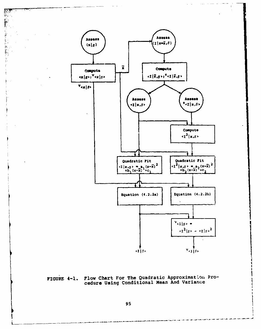
computo caw_

I-- -

Y UlL

n oa2Vxsor

5adratic Pit Qadratic Fit

+bIV< +b• 2 x

v Ills> -¢ I

<12S V <I js ý,

FIGURE 4-1. Flow Chart For The Quadratic Approximatlaoii Pro-cedure Using Conditional Mean And Variance

95

inn

Inn

%n 0.41

0

enQ

0'

04

Ln04)N0

1044

41-

969

change as the revealed value of age increases and decreases from

the mean of the age distribution. Similarly, the standard devia-

tion of income at the mean age provides a benchmark for assessing

the conditional standard deviation as a function of age. The

curves of conditional mean income and income standard deviation

computed for the census data are presented in Figure 4-3.

Of course# the conditional standard deviation is a difficult

concept, and not all decision makers will be able to draw the re-

quired graph, even with the benchmark. It may be necessary to do

additional assessment in order to help the decision maker estimate

the conditional standard deviation. However, if it is necessary

to assess carefully the entire conditional distribution at several

values of the conditioning variable, then the second procedure,

discussed below, should be used.

Once the curves of conditional mean and standard deviation

have been assessed, the conditional second moment can be computed

as a function of the conditioning variable. The conditional second

moment of income given age <I 2 1x,s> is also shown in Figure 4-3.

Each curve, <IIx,S> and <I 2!x,S> , is fit with a quadratic func-

tion and, the coefficients are then used in equation (4.2.2) to

compute the moments of the influenced marginal distribution. For

our example, we have I<IIs> - <IIx,S>+÷Id 2 <L V 2<xls>2 dx2

Ix

= 10350 (-17.3) (126)

= 9260

97

.4 00 0 00 04 00a

-!0!012 I

vIkn k

v 4)

OT

AA

t4J

1 .4 %k

_ x'

0'

0 -A

uNN

94Jo 0 09

$4 H

98

•-.:•j.--+~~~~~ <i2>.<11,>+xrS> VxS

V.1 Is <I--X

dx

. 147 x 10 - (- .494 x 106) (126)

, 116 x 106

azid

.I2 IS> 1 1S> <IS>

, 30.0 x

Procedure II: Assessment of Conditional Distributions

Approximating the age distribution using equation (4.2.3)

requires the assessment of four complete distributions. Figure

4-4 displays a flow chart for this procedure. The necessary

assessments are the marginal age distribution [xIS} and three

distributions for income conditioned on particular values of age.

The conditioning values of age are selected to give a good qua-

.dratic approximation to the age-income surface. For t:mampie, the

following equation works well2 {IlxS} ~ {Ilx= + <xIS>,S-{I Ix=RSfiIx=x,S}-1IIx=i'-<xSS

a xxa<x s ' x I S> .(4.3.1)

0<xIS>

Therefore, the conditioning values of age for the three assessments

of income distribution depend on the mean and standard deviation of

the age distribution.

From the marginal distribution on age (Figure 4-2), the mean

age of.that population is 43.7, and its variance is 126. The three

required distributions of income conditioned on age are shown in

Figure 4-5. These distributions are used in equation (4.3.1) to

99

Assess(Xis

Aasses Assessmsss

Equation (4.3.1)

2iLLia (1x -

FIGURE 4-4. Flow Chart For The Quadratic Approximation Pro-cedure Using Three Conditional Distributions

100

- - ~WWVWrnw W*5UvM% WWW"M Lan"

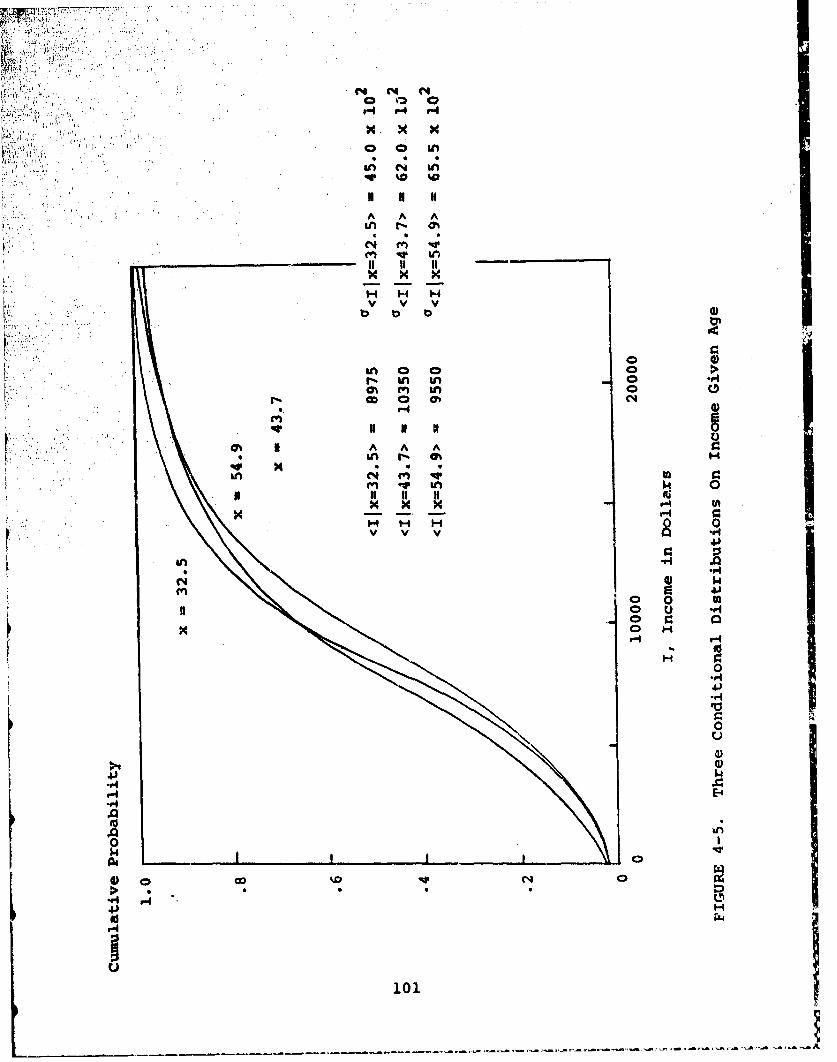
(CM C4 N4

x .x

U; 4 A.

"*1~ 0 0 Sn

r- in4 LoCD 04 '

H H H

A A A

in ~ ~ S C4A4t

M qv M k

H H- 3-4

0 0

Osr- rr)IA0

9-44

U;0 1

* AN

OD S S

>n(4 ~ 4-AA 4

4jI

IA 101

Sf~:2 which In used along with fItx=i,s) inaxx

equation (4.2.3) in obtaining {IISI . Figure 4-6 displays the

uneveness of thG surface (Ilx,S) and also shows the quadratic

approximation to the surface. According to Figure 4-7, the

quadratic approximation for the marginal income distribution

.,closely matches the exact distribution.

The Conventional Procedure: Discrotization

In contrast to the quadratic methods, Figure 4-8 diagrams

the steps in approximating (ils) using the conventional discrete

method. Again, four complete distribtAions must be assessed: the

marginal distribution on age and three conditional income distri-

butions. Following the assessments, each distribution is dis-

cretized to find the expectation in each interval.

The marginal distribution on age used in the discretization

(Figure 4-2) is the same one used for the quadratic approximation.

It is discretized at the points

<xx < 75x,S> = 30

<xl .275 X< X < 8 0 x,S> = 43.7

<xl .80x < x,S> = 60

in order to reduce the amount of data interpolation required. The

notation p refers to the p-fractile of (xiS1 . Conditional

distributions (Ilx,SI are assessed at each of the three ages

given in (4.3.2) and discretized.

In Figure 4-9, the discretization of the age and conditional

income distributions is displayed as an event tree. By taking the

102

'&a

II

SII I.I1.4

V4 44

! in ! •inx H

a

I I AN-I to

LM -r 0

0,4

.2",1

0

1)1to

0

•.0 U,4

E-4

~4J

00

41 0 GDN 0r4 v

>Q1

0 *4

P34

103

4J)

00C)

0 r.

.Q 4 014 i-H 44)4 0 0 4

0 4 4)W4) 14 14 V4

0 u a I1

0d I1?A4

.94

4)1

H -

4144 Od

0 $4

14000 O

414r-4U E-

4J4

to P4

p10

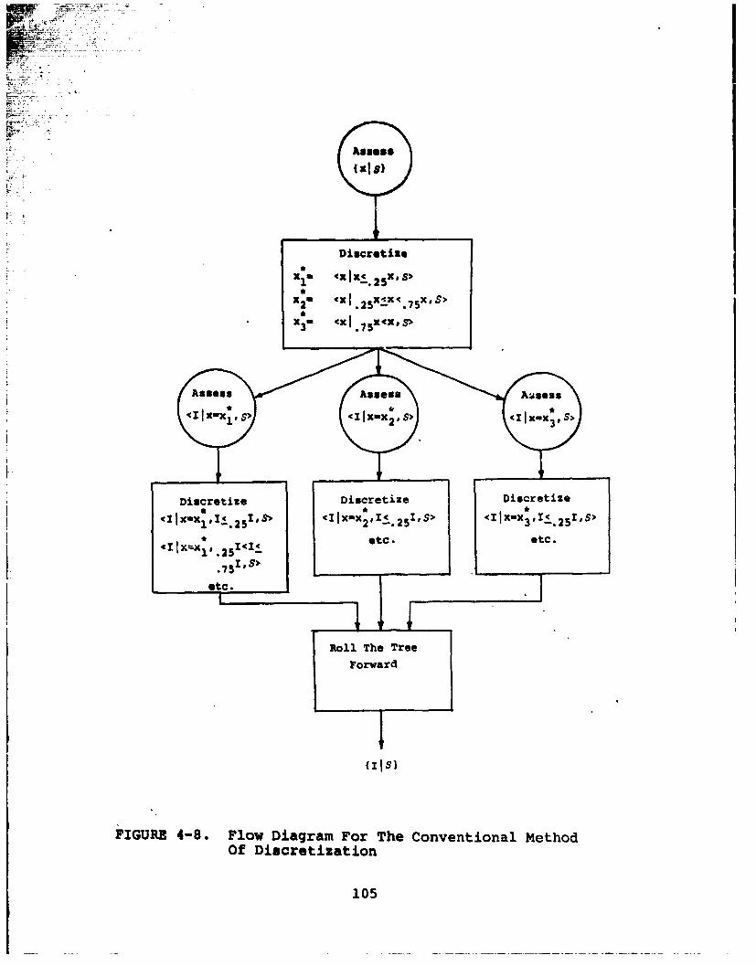
(Assess

Discretizex a- 'ex I X-C 5xS1;x2" •xl, 2 5x.5o

X2 (X 2 5 X1 75xS

13W x. 7 5xcx°s

Discretize Discretize Discretize

otc. etc.V.l~x,25I<•

Roll The TreeForward

{z Is)

FIGURE 4-8. Flow Diagram For The Conventional MethodOf Discretization

105

AGO Income ProductProbability

I " 2900 .069

i x ,,30 _..5 1" 8000

> - , . . (• --- 2 .138

25

~~ I 1.4200.069

I - 3500 .131

S.2

.55x 43.7 .5 1 9250 .6

.263

1 19400 .131

I 1900 .05

Sr = 7900.05

.25

x 60 .5 1 -7000

- .10

.25

I -17900 .05

FIGURtE 4-9. Event Tree Resulting From Discretizdat' Jon

106

ft s n~ a Shfl 1 fl

product of the event trio probabilities, "rolling the tree for-

ward*, the marginal distribution on income can be approximated.

The discrete approximation is plotted along with the quadratic

approximation and the exact distributicn in Figure 4-7.

It is evident from Figure 4-7 that the quadratic approx:ima-

tion is quite accurate, and the discrete approximation is less

accurate. However, the tabulation of Table 4-1, comparing the

moments of the approximation with the exact values, shows the

discrete and continuous approximations to be comparable and

acceptablQ. In the next section the theoretical basis for dis-

cretization is investigated, and the reason for its overestima-tion of the expected income is explained.

4.4 Comparison of Discretization With the Quadratic Approximation

The degree of confidence that we have in a model structure

resulting from influence matrices and our use of the associated

estimate of the profit lottery depends on the accuracy of -he

quadratic approximation. If the approximation is crude, then the

influence matrices can only provide the analyst with a means to

conceptualize the modeling process. The associated estimate of

the profit lottery would need to be verified by more exact methods.

On the other hand, if the quadratic approximation is sufficiently

accurate, then the influence method would yield a model structure

in which the analyst is confident. Furthermore, additional re-

search to determine how to use the estimates of the profit lottery

to solve the decision problem directly from the influence diagram

would be warranted.

107

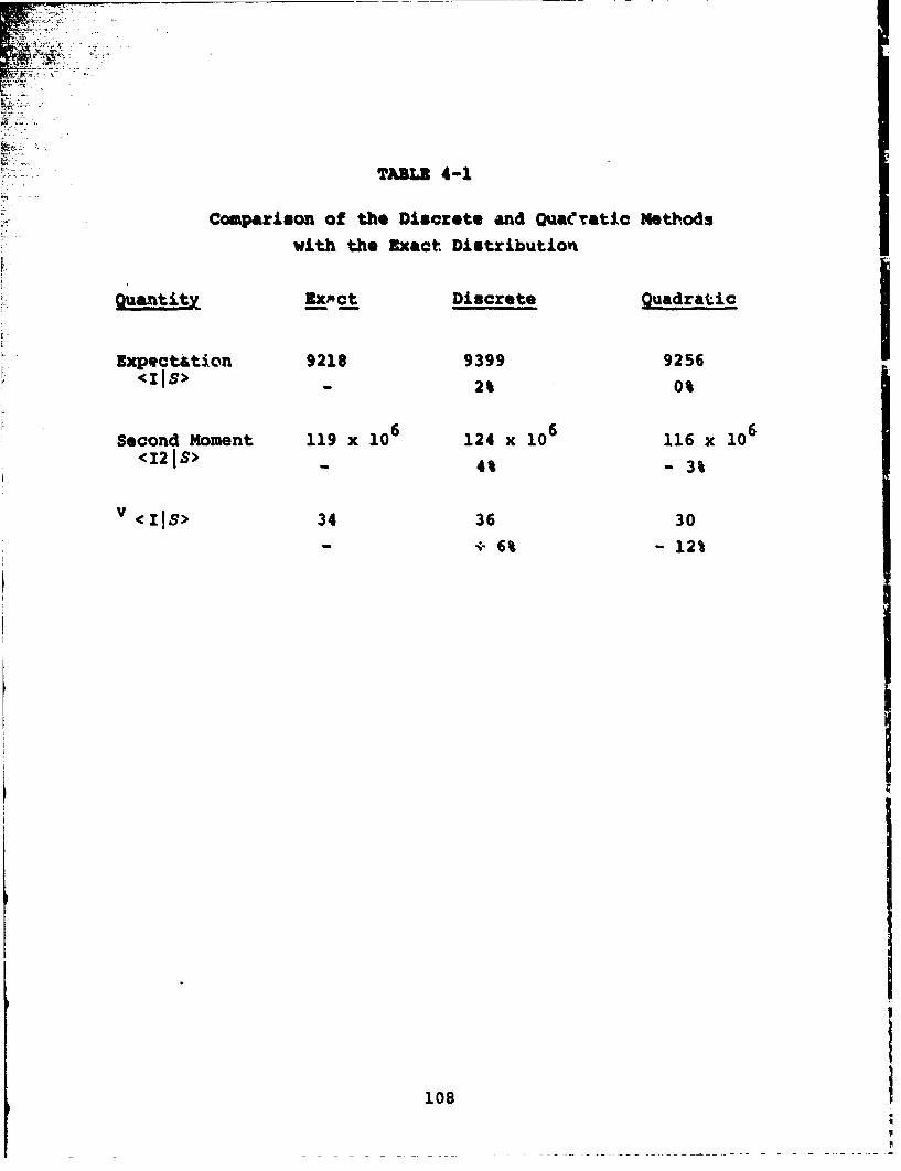
TABut 4-1

Comparison of the Discrete and Quaevratic Methods

with the Exact Distribution

•tilz Exmt Discrete Quadratic

Expectttion 9218 9399 9256<Ils> - 21 0%

Second Moment 119 x 106 124 x 106 116 x 106<12 Is> -4% - 3%

v <I s> 34 36 30

- + 6% -121

108

The most frequently used method for computing the moments

of a distribution that is dependent on another variable is dis-

cretization of the influencing variable. Discretization means

dividing the range of x into intervals and associating tha

probability weight from an interval with a point within that

interval. For example, if {xiS) is a normal distribution, the

analyst can divide x into three intervals at the 25% and 75%

fractiles of NxIS) , denoted 2 5 x and 7 5 x , respectively.

Then, he can assign probability weights of .25, .50, and .25

to the points

<xI - < x < 2 5 x> Z x<xi. 2 5 x 75 .50

< x < Mx>x. 7 5 xx< > .90

This procedure preserves the expectation of Lx IS) , since

<xlS> - <xix <. 25x,S> '{ 2 5xis}

+ <xi. 2 5 x <X <.7 5x,S> [I{. 7 5xiS} - 1{. 2 5xis1I

+ <xl 7 5x<x,S> [1 -•(. 5 xis)]

When (xis) influences {yjS) , the moments of {yls} can

be approximated by repeating the procedure. At each of the points

given in (4.4.1) the analyst discretizes the conditional distri-

bution {yIx,S) . The discretization preserves the moments of

the conditional distribution, since,

< , = <ym . 2 5y,x,s> 1. 25 yjx,S

<ym1.25Y <_Y <.5Yx's> [!'{.75ylx,s} - ''.2,ylx,s}]+<ymI .7,y<_y,xS> [1- <[ Yx')

109 .75- x}]

109

However, the moments of the marginal distribution, (yIS) , are

only approximated au,<¥"Is>-Z <y"Ix-a <=Ix <. K>ts> "€2xls)

~yIS yjx- xi *25205 t 25x 3

(4.4.3) + <ymjx <xl .2 5x 1 x<.?5x>S>'(•. 75xIs) - rk(.2 5xls)l

+ (y*IXUX aX "1~ 9- ' 7 xIs)I+ <ylx <x.7,x <_ "S,>11 75{vsll

or more generallyN+l

(4.4.4) <ymIS> Z ytl <¥ m j x - <Xlxn' 1-x<xnes> ['(x!nls) -'(xn -lS))

where Xo . and X+l ' + .

While discretization of NxIS) preserves the moments of the

state variable distribution (xis) , it only approximates the

moments of the profit lottery (yIS)

An Example Showing that the Moments of the Profit Lotterye-iy~ riiI~i~eFo or Un-g-eres tiatR S--Dlscretiiation

Suppose that (xIS) is a normal distribution with standard

deviation ax and that

<,Ixs> - %xa2 + bmx + cm

Using equation (4.4.3), the approximate value obtained by dis-

cretization at the points of (4.4.1) is<yMID,S> - ama2 + .8 am V<xis> + b; + c.

-2-Since the exact value is ax + bmx + cm , the error due to

discretization is

(4.4.5) <ymlS> - <ymIDS> - * .18 am V<xis>

where. D denotes the value computed using the discretization

procedure. From (4.4.5) the errors in the mean and variance of

(yjs) are found to be

110

(4.4.6) yj$) 4&yDt) - .18 a1 Vcx Svcyls> -v'4yjDs - + .18 a2 V4xlS( - .36 aI v4Ais> <yls>

-.097 aI ~(XIS>

The implioation of these cquations in displayed in Figure

4-10. There will always be an error in the men of the profit

lottery unless al - 0 , and whether it is overestimated orunderestimated depends on the sign of a1 . In either case, thevariance of the profit lottery may be overestimated or underestimated.

Derivation of the Discrete Approximation

These considerations motivate an investigation of the con-

ditionu under which discretization, as in equation (4.4.4), is

exact. We begin with the expansion equation

ad dIi- S> <Ymlx,s> (xls) dx

and divide the integration into regions

(4.4.7) <ymS> - 1f <?ymIx,S>(xls)dx + ... Ix k <ymIxS>xISldx +

S0 k-i+. K <ymlx,S>fxISldx

xK-1

Within each region the conditional moment can be expanded in a

Taylor's series about the expectation of x in that interval,

(4.4.8) <ymlx,s> - <,mIx - <xlxck>,S>

+ 11d (x - <xxxck>cn-i dnx x - <xlxck>

where k - [x: Xk_1 <x<_xk . Substituting (4.4.8) into (4.4.7)

111

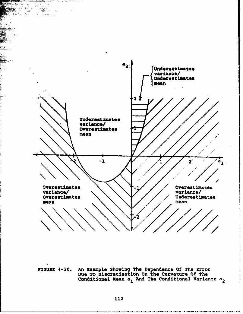
az.a UnderestimatesJvariance/

Stan

2 r

Underestimatesvariance/Overestimatesmean

a

-o / 777

//

Overestimates - / Overestimatesvariance/ variance/Overestimates / Underestimatesmean mean

FIGURE 4-10. An Example Showing The Dependence Of The ErrorDue To Discretization On The Curvature Of TheConditional Mean a1 And The Conditional Variance a2

112

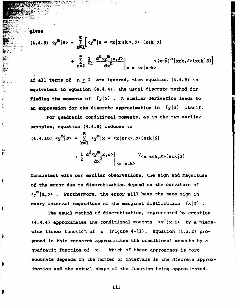
<Y *S -Ca <x Ixek >,,S> (xek S)

S+ ~ <((X-x) xck,S>{xck$S)-

n=2 -* dxn -•-=x <X -<xiek> •

If all terms of n > 2 are ignored, then equation (4.4.9) is

equivalent to equation (4.4.4), the usual discrete method for

finding the moments of {ylS) . A similar derivation leads to

an expression for the discrete approximation to fylS) itself.

For quadratic conditional moments, as in the two earlierc

examples, equation (4.4.9) reduces toK

(4.4.10) <cY mIS> I < <Ix - <xlxck>,S>{xckIS)knl

+ 1 a<Ylx's> V<xlxck,S>[xckjS1dx2 <x!xck>

Consistent with our earlier observations, the sign and magnitude

of thp error due to discretization depend on the curvature of

<Ymlx,S> . Furthermore, the error will have the same sign in

every interval regardless of the marginal distribution NxIS)

The usual method of discretization, represented by equation

(4.4.4) approximates the conditional moments <ymlx,S> by a piece-

wise linear functicn of x (Figure 4-11). Equation (4.2.2) pro-

posed in this research approximates the conditional moments by a

quadratic function of x . Which of these approaches is more

accurate depends on the number of intervals in the discrete approx-

imation and the actual shape of the function being approximated.

113

DiscreteApproximation

n- n +1

~x nS>< l S

FXIGUAZ 4-11. Di~scretizationApproximates Conditional MomentsBy A Piecewise Linear Function

114

We conclude that discretization is not inherently more accurate

than the quadratic method. The better method should be deter-

mined by th4 particular application and the ease of assessment.

115

CHAPTER 5

Summary and Suggestions for

Further Research

Our characterization of influence allows the decision

analyst to conceptualize the relationship between the probability

distributions on different variables in a decision model. One

can think of an influence between two probability distributions

{xjs} and {yl s as transforming the moments of one distribu-

tion into the moments of the other. The strength and type of

the influence can be measured by a set of derivatives denoted

as

(5.1) d<(yý S> >(.1 .<y)I> n > 1, m > 1d< (xx)nI S> I

which extends in an obvious way for n = 1 and m = 1

Therefore, the influence of x on y is characterized by

an infinite matrix that has its n, m element given by (5.1),

and is denoted byd{yIs)

This influence matrix has several useful properties. First, the

matrix is null if and only if the moments of {y IS are unaf-

fected by the moments of {xIS} and y is probabilistically

independent of x . Hence, the matrix is null if and only if no

influence exists. Second, when the matrix has nonzero elements,

those-,elements specify the type and strength of the influence.

Finally, because the elements of the matrix follow the rules of

116

differential calculus, a calculus of influences appears possible.

Pot example, in the diagram:

tha influence matrix of x on z may be computed as

d~ IS). a d(ylS) d~ylS1•

Using several examples, we have demonstrated that inf.-ince

matrices can be used to structure decision problems. The in-

fluence-consequence matrix introduced in Chapter 3 shows that

the elements of the influence matrix can be used to determine

which areas of the decision model require further modeling and

which variables should be treated as uncertain in the decision

model. These recommendations amount to a new interpretation of

deterministic sensitivity.

We have also used the influence matrix to demonstrate that

there is no single correct decision model. The appropriate

decision model depends on the risk attitude of the decision

maker.

Finally, we investigated the theoretical basis for discre-

tizating marginal probability distribut.on!3 to compute the profit

lottery. Discretization and the quadratic method, on which in-

fluence matrices are based, differ only in the assumption about

the functional form of the profit lottery conditioned on the

state variable. Since the two methods are comparable in case of

assessment and accuracy, we conclude that the• quadratic method

117

should be considered as an alternate method for the solution

of decision problems directly from their influence diagrams

without the intermediate step of constructing a decision tree.

To develop this possibility would require extending the

influence theory and influence calculus presented in Chapters

2 and 3 to include decision variables. We illustrate our ap-

proach to this problem with the following example. Consider a

decision variable D influencing the profit lottery {ylD,S}:

Both the mean and variance of the profit lottery will

generally depend on D . Limiting our attention to those two

moments, we write

d<ylD,S>(5.2) <yjDS> Z <yIDOiS> + dD (D - D0 )

DO

+ I 2<(ID,S> (D - 22 dD2 dD ID O0

(5.3) V<yID,S> Z V<yID0,S> + d V<yID'S> (

dD (D - D 0)

Do

118

where D is an arbitrary nominal setting of the decision vari-

able. Let us define the influence of D on {yID,S), analogous

to our earlier definition for the influence between state vari-

ables, as

(5.4) d-~s dcyID,,S> dID0 D jdD "dD DO 0 dD DO0

d 2<,y D,)S > d 2V<yID,S>,2YDD> dD2L dD2LbL I D0 D2 IDo

00

The elements of this matrix can be obtained by an assessment

procedure similar to that discussed in Chapter 4.

Now, the first order condition for the optimum decision

D* is•d-<yls> -

dD D

or approximately

(5d<D,S> 1 dV<yIDpS> -(5 5 cy D S " dD -0 .dD D* D*

Expressions for the two derivatives are obtained by differenti-

ating (5.2) and (5.3). Upon substitution into (5.5), we obtain

an estimate for the difference between D and the optimum de-

cision D*,

(5.6) d<ylD,S> 1 dV<ylD,S>dD D 0 -dD

dDD* D0 2 D2d <yID,S> 1 d V<yD,S>

dD2 D0 2Y dD2 DO

119

Equation (5.6) suggests that the optimal decision can be deter-

mined from the influence of the decision on the profit lottery,

equation (5.4), and the decision maker's risk attitude. In fact,

the right side of equation (5.6) is the ratio of the elements of

the influence vector

(5.7) d . d1 T35 ETY]

Of course, considerable theoretical development is required

to show how to solve general decision problems from the influence

diagram. Our simple example assumes a continuous decision vari-

able, which has derivatives, but in practice decision variables

are often discrete. Furthermore, our simple influence diagram

consists of a single decision variable and a single state variable.

Research is needed to show how to solve sequential decision pro-

blems with several state variables by the influence method. An-

. gsr important related question is how to determine the value of

i1.-rmation directly from the influence diagram.

Our work with the influence method for state variables,

pres,-ited in Chapters 2, 3, and 4, and our simple example in this

ch&. ir, lead us to believe that additional research and experience

with the influence method will lead to more developments of prac-

tical value and theoretical interest. We encourage further re-

search in the application of the influence concept to decision

problems.

120

Refferenoes

[1]. Cook, W. Howard, wDecision Analysis for Product

Development4, IZE Transactions on Systems Sciencean•.d Cbrei--s-Vo . BEC-4It .- ',Spm:• 9

pp. 324-354.

[2]. Hill, J. Doublas and Richard G. Ollila, "Analysisof Complex Decision Making Processes,," IEEE Trans-actions on S syoma. , Man,, and Cybernetic7s-Vo17--C-8,N.3,kiK17, pp. ls 0.;-TO-----

(3]. Howard, Ronald A., "Decision Analysis: Applied DecisionTheory," Proceedings of the Fourth InternationalConferenceo-n Operation~aEResearch, Wiley-Interacience,1966,' Fpp.53--71. '.. .

[4]. Howard, Ronald A., "The Foundations of DecisionAnalysis," IEEE Transactions on Systems Science andCybernetics, Vol. SSC-4, No. 3, September 1968,'pp. 211-279.

[5]. Howard, Ronald A., "Proximal Decision Analysis,"Management Science, Theory, Vol. 17, No. 9, May 1971,pp. 507_-541.

(6]. Howard, Ronald A., J. E. Matheson, and D. W. North,"The Decision to Seed Hurricanes," Science, Vol. 176,16 June 1972, pp. 1191-1202.

[7]. Howard, Ronald A., "Social Decision Analysis,"Proceedings of the IEEE, Vol. 63, No. 3. March 1975,pph 359-371.

[8]. Matheson, James E., "The Economic Value of Analysisand Computation," IEEE Transactions on Sysm Scienceand Cybernetics, SSC-4, No. 3, September 1968,pp. 325-332.

(9]. Matheson, James E., "Decision Analysis Practice:Examples and Insights," Proceedings of the FifthInternational Conference on Operational Research,Venice, 1969, Travistock Publications, 1970,pp. 677-691.

[10]. Miller, Allen C., et al, Development of AutomatedAids for Decision Analysis, Reserc-h Report to theDefse Advanced Research Projects Agency by SRIInternational, Menlo Park, Ca., May 1976, pp. 115-174.

121

(113. Morlan, P. A. P., An Introduction to Probability Theory,Clarendon Press, bNOrf ,T 9611, p. -Yl9.

112]. NOutS, Marcel F., Probability, Allyn and Bacon, Inc.,Boston, 1973, p. 277.

(131. Owen, Daniel L., "Nutual Information as a PotentialDefinition of Influence," unpublished paper.

(143. Pratt, John W., "Risk Aversion in the Small and in theLarge," Econometrica, Vol. 32, No. 1-2, Jinuary-April,1964.

(153. Sag*, Andrew P., Methodoloqy for Large Scale Systems,McGraw-Hill Book Company, New York_-I7,7-pp. 3-164.

(161. Smallwood, R. D., "A Decision Analysis of ModelSelection," IEEE Transactions on Systems Science and" C beretics, V-T. SSC-4, To. 3, September 1968,Tpp.

E17]. Spetzler, Carl S., and Ramon M. Zamora, "DecisionAnalysis of a Facilities Investment and ExpansionProblem," in Readings in Decision Analysis ed. byRonald A. Howard, Jams-E.-Matheson, and KatherineL. Miller, SRI International, Menlo Park, Ca., 1976,pp. 205-233.

[181. Tani, Stephen N., Modeling and Decision Analysis,Ph.D. dissertation, Department of Engineering-EconomicSystems, Stanford University, June 1975.

(191 U. S. Bureau of the Census, Census of Population: 1970Vol. 1, Characteristics of the Popu_-aton Part l,-'•tedStates Summary - Section 2, U. S. Government PrintingOffice, Washington, D.C., 1973.

122

Appendix A

A Series Representation and Approximation for

the Covariance

An expression for Cov(xy) in terms of the moments of

(xiS) can be obtained by writing,

(A.1) Cov(x,y) - )/(x-i) (y-y) {xyS dydx

(A.2) - I (x-i)<ylx,S>{xiSldx

(A.3) " fx<ylx,S>{xlS)dx - ;jx

Expanding <ylxS> in a Taylor's series gives

(A.4) <ylx,s> - <ylx,S> + I n --dxnS> (x-i)n=1 dx-

Upon substitution of (A.4) into (A.2) and completion of the in-

tegration, one obtains

(A.5) Cov(x,y) - 1 d n<y I xS> <(x-_)n+l Is>n 1nI dx n LIx

When <ylx,S> is linear in x, the covariance is equal to

the first term of (A.5),

(A.6) Cov(x,y) =d<ylx,>

x

This expression can be interpreted graphically. Equation

A-1

(A..3) shohs that the oovariance is a comparison of the expected

area cylx,8> x. with the area zy Because of the linearity

of <YlXt > , we have

<Yls> -<Yl;,S>

The variance of (xjS) can be interpreted roughly as an oscilla-

tion of x about <xjS> I and it induces a similar oscillation

of <ylx,S> about <ylxS>. Since the increase in the area

<ylx,S> x is larger when x is greater than x than the cor-

responding reduction when x is less than x, uncertainty in

x increases the expectation of <ylx,S> x. The amount of the

increase of the expectation of <ylx,S>x over y, which by

Equation (A.2) is the covariance, depends on the slope d<ylx,$>dx "

A-2

Increase in x'yjx,t.

whien x >Reduction in x<yJx,S:)

Eyjx,33 vwhenx x

cyjlsI - cylx-i,s, ",

Variation in x aboutits expection

FIGURE A-i. An Interpretation Of The Covariance Using TheApproximation Developed In Appendix A

A- A-3

I- Appendix 9

A proof that the change in the certain equivalent of (xIS)

due to fixing x at its men is approximated by

V ~ 8F- *VCIS, Imv•s

Taking the first two twerma of equation (2.2.2) for m - 1,2

gives

1(8.1) <IS> = <Ix a oS> + hxX V<xIS>

(B.2) <W21s> <12 1xa ;08> + ½h "<,XIs>,

whereh td 2<wlxS>l h: d2<w 2,xS>

xx dx xx dx2

Using (B.1) and (B.2), we obtain

(B.3) v<WIs> - <2jls> - <Is>2

N <cw 2 Ix ;,S>- <Ix ",$>2

2 *+ ( h xx - <vIx - ,S$>h xx 1 h2xx <xlS>)V<XlS>

The approximation for the certain equivalent is

(B.4) "<WIs> - <VIS> - v<WIs>

Using (B.1) and (B..3) in (B.4) yields(B.5) V<WIs> " <RIx - ;,s> - . (<.2 Ix - - >- 2

+ [T h Mhxx -Wlx =x,S>h - Ih2 x- vxS>)VX>

A-4

The first two terms on the right of (B.5) approximate the certain

.quivalent of w when x - x Hence,

(-l.6) "IS• ~<wlx - x,S> 1 [ hx' - ( hx- <nIx=iS>hxx -

-h V<xls>)] V<xls>

According to equation (3.3.3), the influence vector is'

d-x s " [d<7r S> TdxjS [Ld-<x dS> VcxlS>J

"-d{x ) [ T"

The elements of the influence matrix can be found in

Figure 2-4 and used in this equation:[<whS> " h - 2<TrIS> h ] [ - ]T

f hxx Y h*x - <wlS> hx

The second element of this product is

(B.7) d I<xrS> 1 h -h

(B7) d VtxIs> xx -2 2 hxx <71I hx

Substituting for <wlIS> according to B.1,

(B.8) d-<rrS> - 1 h X h * h <n.Ix ixS>hdV<xIS> xx 2 (S >T

1 h 2 v<xS>~xx

Multiplying (B.8) by V<xlS> and comparing with (B.6), we find,

A-5

x IS> - h2 <xls> < 7Is> -><wjl,S>d V<xIs> x

Consequently* the expression

(B.9) d ISlS>d <xls>

approximates the change in the certain equivalent of {wIS} due

to fixing x at its mean value provided the term

Sh2 V<xlS>28 xx

is small. If it is not small it can be added to the expression

(B.9) to improve the -dproximation.

A-6: NZ