Deceptiveness of internet data

for disease surveillance

Reid Priedhorsky*§ Dave Osthus* Ashlynn R. Daughton*†

Kelly R. Moran* Aron Culotta‡*Los Alamos National Laboratory†University of Colorado, Boulder‡Illinois Institute of Technology

§corresponding author: reidpr@lanl.gov

July 30, 2018 / LA-UR 17-24564

Abstract

Quantifying how many people are or will be sick, and where, is a criticalingredient in reducing the burden of disease because it helps the publichealth system plan and implement effective outbreak response. This pro-cess of disease surveillance is currently based on data gathering usingclinical and laboratory methods; this distributed human contact and re-sulting bureaucratic data aggregation yield expensive procedures that lagreal time by weeks or months. The promise of new surveillance approachesusing internet data, such as web event logs or social media messages, isto achieve the same goal but faster and cheaper. However, prior work inthis area lacks a rigorous model of information flow, making it difficult toassess the reliability of both specific approaches and the body of work asa whole.

We model disease surveillance as a Shannon communication. Thisnew framework lets any two disease surveillance approaches be comparedusing a unified vocabulary and conceptual model. Using it, we describeand compare the deficiencies suffered by traditional and internet-basedsurveillance, introduce a new risk metric called deceptiveness, and offermitigations for some of these deficiencies. This framework also makes therich tools of information theory applicable to disease surveillance. Thisbetter understanding will improve the decision-making of public healthpractitioners by helping to leverage internet-based surveillance in a waycomplementary to the strengths of traditional surveillance.

1

arX

iv:1

711.

0624

1v2

[cs

.IT

] 3

1 Ju

l 201

8

1 Introduction

Despite advances in medicine and public health, infectious disease still causessubstantial morbidity and mortality [28]. Disease surveillance provides the datarequired to combat disease by identifying new outbreaks, monitoring ongoingoutbreaks, and forecasting future outbreaks [21]. However, traditional surveil-lance relies on in-person data gathering for clinical evaluations and laboratorytests, making it costly, difficult, and slow to cover the necessary large geographicareas and population. Disease surveillance using internet data promises to reachthe same goals faster and at lower cost.

This promise depends on two things being true: (1) people leave traces of theirown and others’ health status online and (2) these traces can be extracted andused to accurately estimate disease incidence. Traces include search queries [16],social media messages [8], reference work usage [13], and blog posts [7].1

The first claim is compelling, but the second is more elusive. For example, GoogleFlu Trends, a web system based on [16], opened to great fanfare but proved tobe inaccurate in many situations [25] and shut down in the summer of 2015 [11].The field has also encountered difficulty answering criticisms from the publichealth community on how it deals with demographic bias, media coverage ofoutbreaks, high noise levels, and other issues. Because the field’s successes arebased on observational studies in specific contexts, it is hard to know how robustor generalizable these approaches are or what unsuccessful alternatives remainunpublished.

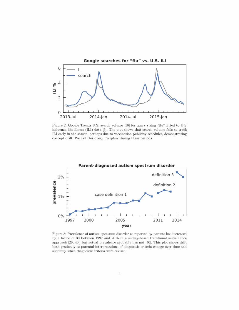
This paper argues that a necessary part of the solution is a mathematical modelof the disease surveillance information flow. We offer such a model, describingboth internet-based and traditional disease surveillance as a Shannon commu-nication [37] (Figure 1). This lets us discuss the two approaches with unifiedvocabulary and mathematics. In particular, we show that they face similar chal-lenges, but these challenges manifest and are addressed differently. For example,both face concept drift [12]: Google search volume is sometimes, but not always,predictive of influenza incidence (Figure 2), and traditional estimates of autismspectrum disorder are impacted by changing interpretations of changing casedefinitions [40] (Figure 3).

Using this model, we introduce a new quality metric, deceptiveness, in order toquantify how much a surveillance system risks giving the right answer for thewrong reasons, i.e., to put a number on “past performance is no guarantee offuture results”. For example, basketball-related web searches correlate with someinfluenza seasons, and are thus predictive of flu, but should not be included influ estimation models because this correlation is a coincidence [16].

This approach lets us do three things. First, we show that neither approachis perfect nor has fully addressed its challenges. Second, we show that the two

1One review of this body of research is our previous work [32].

2

+

INFORMATION SOURCE

populationat risk

ENCODER care provider assignment

internet system and users

DESTINATION public health leadership

DECODER weighted average

statistical model

NOISE SOURCE health care system

internet system and users

MESSAGE w disease incidence

RECEIVED MESSAGE ŵ incidence estimate

SIGNAL U

incidence by sub-population some internet activity traces

RECEIVED SIGNAL X

diagnoses by sub-population all internet activity traces

NOISE systematic δ random ε

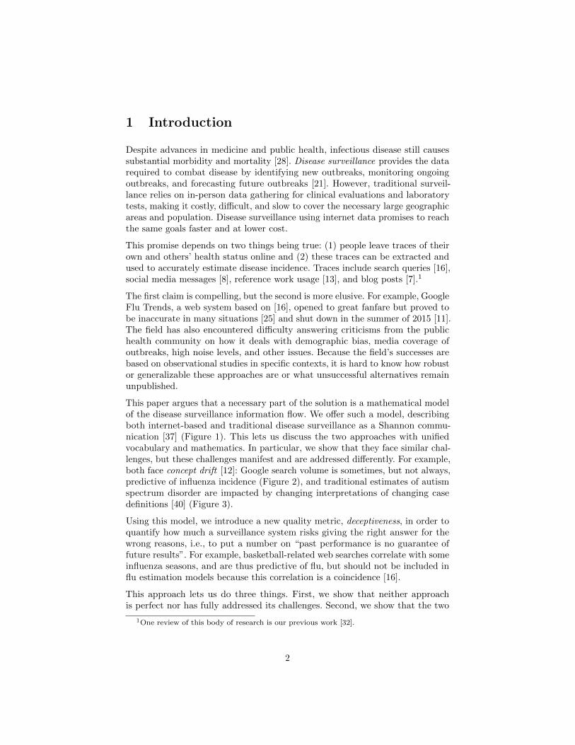
Figure 1: Schematic diagram of disease surveillance as a Shannon communication,patterned after Figure 1 of [37] and using the notation in this paper. This formulationlets one compare any two disease surveillance approaches with unified vocabulary andapply the rich tools of information theory.

approaches are complementary; internet-based disease surveillance can add valueto but not replace traditional surveillance. Finally, we identify specific improve-ments that internet-based surveillance can make, in order to become a trustedcomplement, and show how such improvements can be quantified.

In the body of this paper, we first describe a general mapping of disease surveil-lance to the components of Shannon communication, along with its challengesand evaluation metrics in terms of this mapping. We then cover the same threeaspects of traditional and internet-based surveillance more specifically. We closewith a future research agenda in light of this description.

2 Disease surveillance in general

Many aspects of traditional and internet-based disease surveillance are similar.This section lays out the bulk of our model in common and highlights the aspectsthat will be treated specifically later. We first describe disease surveillance asa Shannon communication, then use these concepts to discuss the challenges ofsurveillance and metrics to assess performance.

3

2013-Jul 2014-Jan 2014-Jul 2015-Jan0

2

4

6

ILI %

Google searches for flu vs. U.S. ILI

ILIsearch

Figure 2: Google Trends U.S. search volume [18] for query string “flu” fitted to U.S.influenza-like-illness (ILI) data [6]. The plot shows that search volume fails to trackILI early in the season, perhaps due to vaccination publicity schedules, demonstratingconcept drift. We call this query deceptive during these periods.

1997 2000 2005 2011 2014year

0%

1%

2%

prev

alen

ce

case definition 1

definition 2

definition 3

Parent-diagnosed autism spectrum disorder

Figure 3: Prevalence of autism spectrum disorder as reported by parents has increasedby a factor of 30 between 1997 and 2015 in a survey-based traditional surveillanceapproach [29, 40], but actual prevalence probably has not [40]. This plot shows driftboth gradually as parental interpretations of diagnostic criteria change over time andsuddenly when diagnostic criteria were revised.

4

25 people in population5 infected this week (20%)

2/6 are diagnosed (33%)

Incidence estimate isweighted mean:2/6 × 10/25 + 3/8 × 15/25 = 36%

Article coefficients trained on previous reference data𝛽₃ = 0.023 Influenza𝛽₂ = 0.016 Fever𝛽₁ = 0.000 Basketball𝛽₀ = 0.090 intercept

Update coefficientsfor next time

10 use Clinic A  1 infected (10%)

15 use Clinic B  4 infected (27%)

6 visit clinic

3/8 are diagnosed (38%)

8 visit clinic

information source messagesignalencoder

received signalnoise source

"

Wikipedia article Influenza

3 visits from infection observations

3 visits for other reasons

" " "

" "6 visits total

"

Wikipedia article Fever

3 visits from infection observations

4 visits for other reasons

" " "

" "7 visits total

"

"×

"

Wikipedia article Basketball

1 visits from infection observations

4 visits for other reasons

"

" "5 visits total

"

signal encoder and noise source received signal

decoderreceived message

Apply statistical model6𝛽₃ + 7𝛽₂ + 5𝛽₁ + 𝛽₀6×0.024 + 7×0.016 + 5×0 + 0.090 = 34%

decoder

#destination

received message

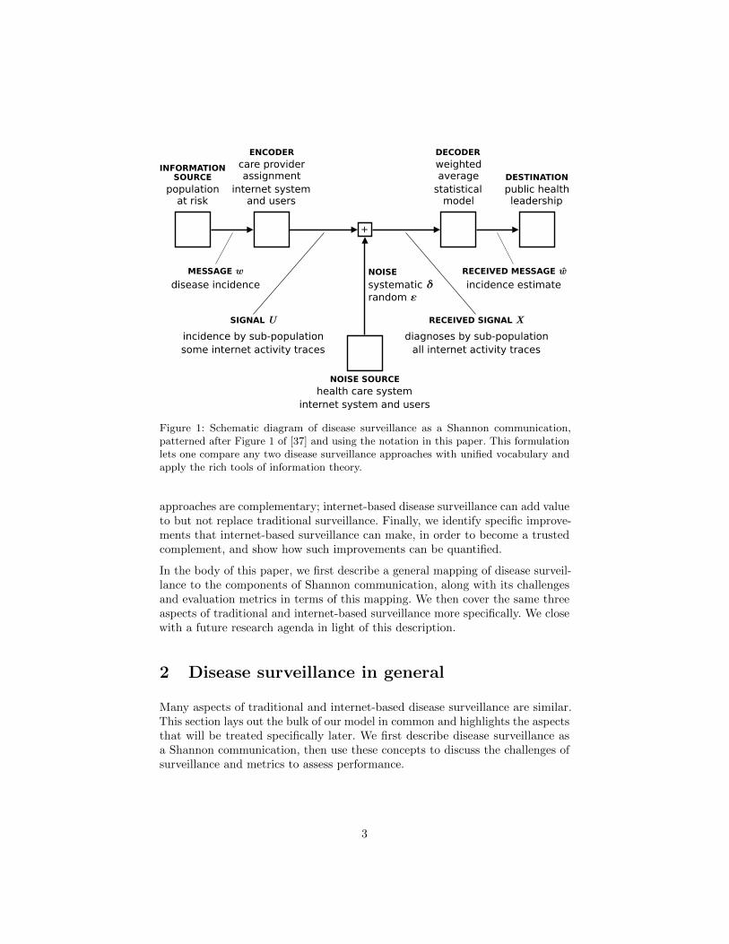
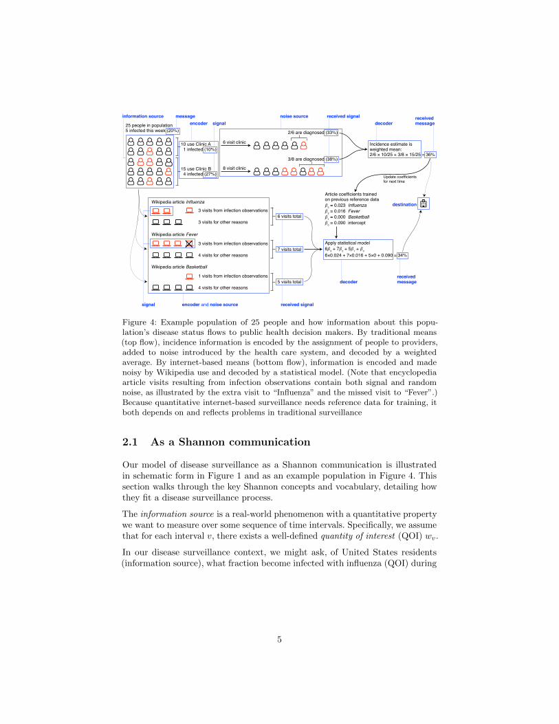
Figure 4: Example population of 25 people and how information about this popu-lation’s disease status flows to public health decision makers. By traditional means(top flow), incidence information is encoded by the assignment of people to providers,added to noise introduced by the health care system, and decoded by a weightedaverage. By internet-based means (bottom flow), information is encoded and madenoisy by Wikipedia use and decoded by a statistical model. (Note that encyclopediaarticle visits resulting from infection observations contain both signal and randomnoise, as illustrated by the extra visit to “Influenza” and the missed visit to “Fever”.)Because quantitative internet-based surveillance needs reference data for training, itboth depends on and reflects problems in traditional surveillance

2.1 As a Shannon communication

Our model of disease surveillance as a Shannon communication is illustratedin schematic form in Figure 1 and as an example population in Figure 4. Thissection walks through the key Shannon concepts and vocabulary, detailing howthey fit a disease surveillance process.

The information source is a real-world phenomenon with a quantitative propertywe want to measure over some sequence of time intervals. Specifically, we assumethat for each interval v, there exists a well-defined quantity of interest (QOI) wv.

In our disease surveillance context, we might ask, of United States residents(information source), what fraction become infected with influenza (QOI) during

5

each week of the flu season (interval):2

wv =people newly infected during v

total population at risk(1)

Each wv comprises one symbol, and the message W is the sequence of all wv;i.e., W = {w1, w2, ..., w|V |}. Here, W comprises the true, unobservable epidemiccurve [30] that public health professionals strive for.

Next, each symbol is transformed by an encoder function to its correspondingencoded symbol, Uv(wv). This transformation is distributed, so Uv is not a scalarquantity but rather a set of sub-symbols uvi:

Uv(wv) = {uv1(wv), uv2(wv), . . . , uv|U |(wv)} (2)

(Note that when clear from context, we use unadorned function names like Uv anduv to refer to their output, not the function itself, with the argument implied.)

For traditional disease surveillance, the encoder is the partitioning of the pop-ulation at risk into sub-populations. For example, uvi might be the fraction ofpeople served by clinic i who became infected during interval v.

For internet-based surveillance, the encoder is an internet system along withits users. Individuals with health concerns search, click links, write messages,and create other activity traces related to their health status or observations.For example, uvi might be the noise-free number of web searches for query imotivated by observations of infection.

Both types of disease surveillance are noisy. Thus, Uv is unobservable by thedecoder. Instead, the received symbol at each interval is a set Xv of noisy features:

xvi(wv) = uvi(wv) + δvi + εvi (3)

Xv(wv) = {xv1(wv), xv2(wv), . . . , xv|U |(wv)} (4)

Each observable feature xvi is composed of unobservable signal uvi, systematicnoise δvi, and random noise εvi.

For traditional disease surveillance, the noise source is the front-line health caresystem along with individuals’ choices on whether to engage with this system.For example, there is random variation in whether an individual chooses toseek care and systematically varying influence on those choices. Also, diagnosticcriteria can be over- or under-inclusive, and providers make both random andsystematic diagnosis errors. Considering these and other influences, xvi mightbe the fraction of individuals visiting clinic i who are diagnosed positive during

2This is known as incidence. An alternate measure is prevalence, which is the number ofactive infections at any given time and which may be more observable by laypeople. Despitethis, we illustrate our model with incidence because it is more commonly used by public healthprofessionals. The two are roughly interchangeable unless the interval duration is considerablyshorter than the typical duration of infection.

6

interval v, which is not the same as the fraction of individuals in sub-populationi who become infected.

For internet-based surveillance, both the noise source and the encoder are inthe internet system and its users. For example, whether a given individual withhealth observations makes a given search contains random variation and system-atic biases; also, health-related articles are visited by individuals for non-healthreasons. Technical effects such as caching also affect the data. xvi might be thenumber of number of searches for query i, which is different than the numberof searches for query i motivated by observations of infection and unaffected bynoise.

The decoder function wv(Xv) transforms the received symbol into an estimate ofthe QOI. For traditional disease surveillance, this is typically a weighted averageof xvi; for internet-based surveillance, it is a statistical model trained againstavailable traditional surveillance estimates, which lag real time.

Further details of encoding, noise, and decoding are specific to the differentsurveillance methods and will be explored below.

Finally, the destination of the communication is the people who act on theknowledge contained in wv, in our case those who make public health decisions,such as public health professionals and elected or appointed leadership.

The problem is that wv 6= wv for both traditional and internet surveillance. Thisleads to the questions why and by how much, which we address next.

2.2 Challenges

QOI estimates wv are inaccurate for specific reasons.3 Feature i might be non-useful because (a) uvi(Xv) is too small, (b) δvi is too large, (c) the function uviis changing, and/or (d) δvi is changing. These problems can be exacerbated bymodel misspecification, e.g. if the “true” relationship is quadratic but a linearmodel is used; we assume a reasonably appropriate model. The following sub-sections describe these four challenges.

2.2.1 uvi(Xv) too small: Signal to noise ratio

Disease surveillance can miss useful information because the signal uvi is toosmall: either it does not exist (uvi = 0) or is swamped by noise (uvi � δvi + εvi).

3This ontology of errors is related to that of survey statistics, which classifies on twodimensions [24]. Sampling error is random when the whole population is not observed andsystematic when the selected sample is non-representative (selection bias). Non-sampling erroris everything else, such as measurement and transcription error, and can also be random orsystematic.

7

For example, many diseases have high rates of asymptomatic infection; abouthalf of influenza cases have no symptoms [4]. Asymptomatic infections are hardto measure because they do not motivate internet traces and infected individualsdo not seek care. Thus, correction factors tend to be uncertain, particularly forspecific outbreaks.

An example of the latter is diseases that have low incidence but are well-knownand interesting to the public, such as rabies, which had two U.S. cases in 2013 [1].These diseases tend to produce many internet activity traces, but few are relatedto actual infections.

2.2.2 δvi too large: Static sample bias

The populations sampled by disease surveillance differ from the population atlarge in systematic ways. For example, those who seek care at clinics, and arethus available to traditional surveillance, tend to be sicker than the generalpopulation [19], and internet systems invariably have different demographicsthan the general population [10].

This problem increases systematic noise δvi for a given feature i by the sameamount in each interval v.

2.2.3 uvi changing: Encoding drift

The encoder function can change over time, i.e., uvi 6= uti for different intervalsv 6= t. For example, internet systems often grow rapidly; this increases thenumber of available observers, in turn increasing the average number of tracesper infection.

This is a form of concept drift and reduces estimate accuracy when modelserroneously assume function uvi = uti.

2.2.4 δvi changing: Sample bias drift

Systematic noise can also change over time, i.e., δvi 6= δti. A commonly citedcause is the “Oprah Effect” (named after the American television personalityand businesswoman Oprah Winfrey), where public interest in an outbreak risesdue to media coverage, in turn driving an increase in internet activity relatedto this coverage rather than disease incidence [3]. Traditional surveillance canhave similar problems, dubbed the “Jolie Effect”; some scholars believe actressAngelina Jolie’s well-publicized preemptive mastectomy caused a significantchange in the population of women seeking breast cancer-related genetic tests [9].

This is another form of concept drift and reduces estimate accuracy when modelserroneously assume δvi = δti.

8

Some phenomena can be a mix of the two types of drift. For example, internetsystems actively manipulate activity [25], such as Google’s search recommen-dations that update live while a query is being typed [17]. This can lead usersto create disease-related activity traces they might not have otherwise, whethermotivated by an observed infection (encoding drift) or not (sample bias drift).

2.3 Accuracy metrics

Epidemiologists evaluate disease surveillance systems on a variety of qualitativeand quantitative dimensions [38]. One of these is accuracy: how close is theestimated incidence to the true value? This can be considered from two perspec-tives. Error is the difference between the estimated and true QOI values, whiledeceptiveness is the fraction of an estimate that is based on coincidental ratherthan informative evidence. The latter is important because it quantifies the riskthat future applications of a model will give less accurate estimates. This sectiondefines the two metrics.

2.3.1 Error

We quantify error E in the usual way, as the difference between the QOI and itsestimate:

Ev = wv − wv (5)

Perfectly accurate estimates yield Ev = 0, overestimates Ev > 0, and underesti-mates Ev < 0. Importantly, Ev is unobservable, because wv is unobservable.

As we discuss below, traditional surveillance acknowledges that Ev 6= 0 but itsmethods often assume Ev = 0, and this finds its way into internet surveillancevia the latter’s training.

2.3.2 Deceptiveness

Our second metric, deceptiveness, addresses the issue that an estimate can beaccurate for the wrong reasons. A deceptive search query is illustrated in Figure 2.Another example for internet-based surveillance is the sport of basketball, whoseseason of play roughly coincides with the flu season. A naıve model can noticethis correlation and build a decoder that uses basketball-related activity tracesto accurately estimate flu incidence. Philosophers might say this model has ajustified true belief — it has a correct, evidence-based assessment of the flu —but this belief is not knowledge because it is not based on relevant evidence,creating a Gettier problem [14]. This flu model relies on a coincidental, ratherthan real, relationship [16]. We call such a model, based on deceptive features,also deceptive.

9

We quantify the deceptiveness of both disease incidence estimates and individualfeatures for both specific intervals and the analysis period as a whole. For aspecific interval, deceptiveness is the fraction of the feature or estimate’s valuethat is the result of noise, and the deceptiveness for the analysis period as a wholeis the maximum of any interval (or some other suitable aggregation function).

Specifically, the deceptiveness of a specific feature i at interval v is:4

gvi =|δvi|+ |εvi|

|uvi|+ |δvi|+ |εvi|∈ [0, 1] (6)

One can also define systematic and random deceptiveness gs and gr if the twotypes of noise should be considered separately.

We summarize the deceptiveness of a feature by its maximum deceptiveness overall intervals:

gi = maxv

(gvi) (7)

The deceptiveness of a complete estimate or model depends on the decoderfunction w, because a decoder that is better able to exclude noise (e.g., by givingdeceptive features small coefficients) will reduce the deceptiveness of its estimates.Thus, we partition w into functions that depend on signal ws, systematic noisewns, and random noise wnr:

∆v = {δv1, δv2, ..., δv|U |} (8)

Ev = {εv1, εv2, ..., εv|U |} (9)

wv(Xv) = wsv(Uv) + wns

v (∆v) + wnrv (Ev) (10)

The deceptiveness of an estimate G is therefore:

Gv =|wns

v (∆v)|+ |wnrv (Ev)|

|wsv(Uv)|+ |wns

v (∆v)|+ |wnrv (Ev)|

∈ [0, 1] (11)

G = maxv

(Gv) (12)

A deceptive feature is an example of a spurious relationship. These typicallyarise due to omitted variable bias: there is some confounding variable (e.g., dayof year) that jointly influences both a deceptive feature and the QOI, creating amodel mis-specification [2]. Corrections include adding confounds to the modelas control variables and data de-trending. These effects can be captured by ourapproach in wns and wnr.

Like error, deceptiveness is unobservable, and more pernicious because quan-tifying it relies on the causality of the relationship between a feature and theQOI. This makes it easy and tempting to discount. Further, being a measure of

4This formulation ignores the fact that a feature can have multiple, offsetting sources ofnoise. One could correct this problem by summing the absolute value of each noise sourceindependently. In general, the definition of g should be adapted to specific applications.

10

risk, estimating it from past data requires care because relevant future outcomescannot be incorporated. However, as we discuss below, additional informationsuch as semantic relatedness can help with such estimates.

We turn next to a specific analysis of traditional disease surveillance as a Shannoncommunication.

3 Traditional disease surveillance

Traditional disease surveillance is based on in-person gathering of clinical orlaboratory data. These data feed into a reporting chain that aggregates themand computes the corresponding QOI estimates.

This section completes the Shannon model for traditional surveillance by detail-ing the encoding, noise, and decoding steps. We then explore the implicationsof this model for the surveillance challenges and accuracy metrics.

3.1 Shannon communication model

As a concrete example to illustrate the encoding and decoding componentsof the traditional surveillance communication, we use the United States’ sea-sonal influenza reporting system, ILInet, because it is one of the most fea-tureful traditional surveillance systems. ILInet produces incidence estimates ofinfluenza-like-illness (ILI): symptoms consistent with influenza that lack a non-flu explanation [5]. Other well-known surveillance systems include the EuropeanSurveillance System (TESSy) [31], the Foodborne Diseases Active SurveillanceNetwork (FoodNet) [20], and the United States’ arboviral surveillance system(ArboNET) [27].

Data for ILInet is collected at roughly 2,800 voluntarily reporting sentinelprovider clinics [5]. During each one-week interval, reporting providers count(a) the total number of patients seen and (b) the number of patients diagnosedwith ILI. These numbers are aggregated via state health departments and theCDC to produce the published ILI estimates.

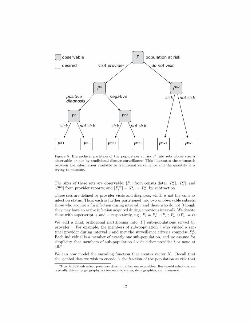
This procedure suggests a hierarchical partition of the population at risk, asillustrated in Figure 5. The observable sets are:

• Pv : All members of the population at risk.

• P vv : People who visit a sentinel provider.

• P nvv : People who do not visit a sentinel provider.

• P dv : People who visit a provider and meet the surveillance criteria, in this

case because they are diagnosed with ILI.

• P ndv : People who visit a provider but do not meet the surveillance criteria.

11

Pd+ Pd– Pnd+ Pnd– Pnv+ Pnv–

Pd Pnd

PnvPv

Pobservable

desired

population at risk

visit provider do not visit

positive diagnosis

negative sick not sick

sick not sick sick not sick

Figure 5: Hierarchical partition of the population at risk P into sets whose size isobservable or not by traditional disease surveillance. This illustrates the mismatchbetween the information available to traditional surveillance and the quantity it istrying to measure.

The sizes of these sets are observable: |Pv| from census data; |P vv |, |P d

v |, and|P nd

v | from provider reports; and |P nvv | = |Pv| − |P v

v | by subtraction.

These sets are defined by provider visits and diagnosis, which is not the same asinfection status. Thus, each is further partitioned into two unobservable subsets:those who acquire a flu infection during interval v and those who do not (thoughthey may have an active infection acquired during a previous interval). We denotethese with superscript + and − respectively, e.g., Pv = P+

v ∪P−v ; P+v ∩P−v = ∅.

We add a final, orthogonal partitioning into |U | sub-populations served byprovider i. For example, the members of sub-population i who visited a sen-tinel provider during interval v and met the surveillance criteria comprise P d

vi.Each individual is a member of exactly one sub-population, and we assume forsimplicity that members of sub-population i visit either provider i or none atall.5

We can now model the encoding function that creates vector Xv. Recall thatthe symbol that we wish to encode is the fraction of the population at risk that

5How individuals select providers does not affect our exposition. Real-world selections aretypically driven by geography, socioeconomic status, demographics, and insurance.

12

became infected during the interval:

wv =|P+

v ||Pv|

(13)

|P+v | = |P d+

v |+ |P nd+v |+ |P nv+

v | (14)

This can be partitioned by sub-population i:

uvi(wv) =|P+

vi ||Pvi|

(15)

βi =|Pvi||Pv|

(16)

wv =

|U |∑i=1

βiuvi (17)

Note that wv is defined in terms of infection status. On the other hand, surveil-lance can observe only whether someone visits a sentinel provider and whetherthey are diagnosed with the surveillance criteria. Each feature xvi ∈ Xv is thefraction of patients visiting provider i who are diagnosed:6

xvi =|P d

vi||P v

vi|(18)

Decoding to produce the estimate wv is accomplished as in Equation 17, usingthe population-derived β as above:7

w(Xv) =

|U |∑i=1

βixvi (19)

In short, the traditional surveillance communication is purpose-built to col-lect only disease-relevant information and thus couples with a simple decoder.Nonetheless, this communication does face the challenges enumerated above andis not noise-free. This we address next.

3.2 Challenges

This section details the four challenges outlined above in the context of traditionalsurveillance. The key issue is sample bias, both static and dynamic.

6In reality, providers report the numerator and denominator of xvi separately, but we omitthis detail for simplicity.

7This corresponds to the ILInet product weighted ILI, which weights by state population.A second product, plain ILI, gives each reporting provider equal weight. For simplicity, thispaper uses unadorned ILI to refer to weighted ILI.

13

3.2.1 Signal to noise ratio

Traditional surveillance generally does not have meaningful problems with signalto noise ratio. While there are noise sources, as discussed below, these tend tobe a nuisance rather than a cause of misleading conclusions.

This is due largely to the purpose-built nature of the surveillance system, whichworks hard to measure only what is of interest. To avoid missing cases of impor-tant rare diseases, where signal to noise ratio is of greatest concern, monitoringis more focused. For example, any provider who sees a case of rabies must reportit [1], in contrast to ILInet, which captures only a sample of seasonal flu cases.

3.2.2 Static sample bias

Patient populations (P v) differ systematically from the general population (P ).For example, patients in the Veteran Health Administration tend to be sickerand older than the general population [19], and traditional influenza systemstend to over-represent severe cases that are more common in children and theelderly [35].

Sampling bias can in principle be mitigated by adjusting measurement weightsto account for the ways in which the populations differ, for example by age [35],triage score [35], and geography [5]. This, however, requires quantitative knowl-edge of the difference, which is not always available or accurate.

ILInet uses the number of sites that report each week, state-specific baselines,and age [5]. For influenza, age is particularly important for mitigating samplebias, because severity and attack rate differ widely between age groups [35].

3.2.3 Encoding drift

In our model, traditional surveillance is immune to encoding drift because theencoder functions contain only wv (Equation 15); there are no other parametersto effect drift.

3.2.4 Sample bias drift

Traditional surveillance is designed to be consistent over time, but it does notreach this goal perfectly and is not immune to drifting sample bias.

One source of drift is that case definitions change. Figure 3 illustrates this forautism spectrum disorder, and the definition of ILI has also varied over time [23].Another is that individuals’ decisions on whether to seek care drift; for example,media coverage of an outbreak [34] or a celebrity editorial [9] can affect these

14

decisions. These and others do not affect the newly infected and non-newly-infected equally, so the sample bias and associated systematic noise changes.

This suggests that traditional surveillance might be improved by better address-ing sample bias. Bias could be reduced by sampling those not seeking care, e.g.,by random telephone surveys of the general population for flu symptoms, and itcould be better corrected with improved static and dynamic bias models.

3.3 Accuracy

Traditional surveillance features include patients not newly infected (P d−vi ⊂ P d

vi)and exclude people who are newly infected but receive a negative diagnosis or donot visit a sentinel provider (P nd+

vi ∩P dvi = ∅ and P nv+

vi ∩P vvi = ∅, respectively).

Causes include lack of symptoms, diagnosis errors by individual or provider, andaccess problems. That is:

xvi =|P d

vi||P v

vi|6= |P

+vi ||Pvi|

= uvi (20)

In practice, this problem is addressed by essentially assuming it away. Thatis, consumers of traditional surveillance assume that the fraction of patientsdiagnosed with the surveillance criteria does in fact equal the new infection rateamong the general population:

|P dvi||P v

vi|=|P+

vi ||Pvi|

(21)

xvi = uvi (22)

Some recent work extends this to assume that the quantities are proportional,independent of v [36, e.g.].

Epidemiologists know this assumption is dubious. They are careful to refer to“ILI” rather than “influenza”, do not claim that ILI is equal to incidence, andgive more consideration to changes over time rather than specific estimate values.Under these caveats, the measure serves well the direct goals of surveillance, suchas understanding when an outbreak will peak and its severity relative to pastoutbreaks [5].

Both error and deceptiveness in traditional surveillance depend on noise. Thiscan be quantified by rewriting Equation 18:

xvi = uvi +|P d

vi||P v

vi|− |P

+vi ||Pvi|

(23)

δvi + εvi =|P d

vi||P v

vi|− |P

+vi ||Pvi|

(24)

15

As one might expect, the noise in feature xvi is the difference between the fractionof clinic-visiting, diagnosed patients and the fraction of the general populationnewly infected.

One challenge is separating the noise into systematic and random components.For example, if a newly infected person chooses to seek care, how much of thatdecision is random chance and how much is systematic bias? The present workdoes not address this, but one can imagine additional parameters to quantifythis distinction.

3.3.1 Error

Recall that error is the difference between the true QOI and its estimate:

Ev = wv −|P+

v ||Pv|

(25)

The unobservable ratio|P+

v ||Pv| can be estimated, but with difficulty, because one

must test the entire population, not just those who seek care or are symptomatic.One way to do this is a sero-prevalence study, which looks for antibodies inthe blood of all members of a population; this provides direct evidence of pastinfection rates [15].

The adjustments discussed above in §3.2 also reduce error by improving wv.

3.3.2 Deceptiveness

One can write the deceptiveness of a specific feature as follows:

gvi =

∣∣∣ |Pdvi||P v

vi|− uvi

∣∣∣uvi +

∣∣∣ |Pdvi||P v

vi|− uvi

∣∣∣ (26)

Note that because we only know δvi and εvi as a sum, we must use |δvi+εvi| ratherthan |δvi|+ |εvi|, making the metric less robust against offsetting systematic andrandom error.

This again depends on an unobservable ratio, meaning that in practice it mustbe estimated rather than measured.

wv 6= wv in traditional disease surveillance due to unavoidable systematic andrandom noise. Nevertheless, it frequently provides high-quality data of greatsocial value. For example, the distinction between a case of influenza and a caseof non-influenza respiratory disease with flu-like symptoms is often immaterialto clinical resource allocation and staffing decisions, because the key quantity isvolume of patients rather than which specific organism is at fault. wv provides

16

this. Thus, traditional surveillance is an example of a situation where the quantityof interest wv is elusive, but a noisy and biased surrogate wv is available andsufficient for many purposes. Accordingly, traditional surveillance has much incommon with internet-based surveillance, as we next explore.

4 Internet-based disease surveillance

In contrast to traditional surveillance, which is based on data gathered by directobservation of individual patients, internet-based disease surveillance conjecturesthat traces of people’s internet activity can drive a useful incidence estimationmodel. Thus, its Shannon communication differs, as do the corresponding impli-cations for its challenges and accuracy.

4.1 Shannon communication model

Internet-based surveillance leverages found features optimized for unrelated pur-poses,8 instead of purpose-built ones as in traditional surveillance.

Rather than diagnosis counts made by health care providers, features in internetsurveillance arise by counting defined classes of activity traces; thus, they aremuch more numerous. For example, Wikipedia contains 40 million encyclopediaarticles across all its languages [41], versus 2,800 ILInet providers. As a corol-lary, while traditional features offer useful information by design, internet-basedfeatures are the result of complex guided and emergent human behavior andthus overwhelmingly non-informative. That is, most internet features provideno useful information about flu incidence, but a few might. For example, thenumber of times the Wikipedia article “Influenza” was requested in a given weekplausibly informs a flu estimate, while “Basketball” and “George H. W. Bush”do not.

Raw traces such as access log lines are converted into counts, such as the numberof requests for each article, searches for each query string, or n-gram mentionsper unit time. In the case of Wikipedia, xvi ∈ Z ≥ 0 is the number of requestsfor Wikipedia article i during interval v.

These trace counts comprise the features. For example, for each new infectionduring interval v, some number of requests uvi for every Wikipedia article i isgenerated. Added to this signal is systematic noise δvi (article requests made forother reasons), and random noise εvi (random variation in article traffic). Thus,the features observable to the decoder are the familiar mix of signal and noise:

xvi = uvi + δvi + εvi. (3)

8For example, looking at illustrations of cats [33].

17

Internet features use a different unit than traditional features. For traditionalsurveillance, the symbol and feature units are both the person, who has a specificinfection status and can be assigned a positive or negative diagnosis. For internetsurveillance, the unit is activity traces. These include traces of informationseeking activity such as Wikipedia article requests [13] or Google searches [16]as well as information sharing activity such as n-grams in Twitter messages [8].This mismatch between feature units (trace counts) and encoded symbol units(people) is a challenge for internet-based surveillance that is not shared withtraditional surveillance.

Like traditional surveillance, the decoder is a function of the observable data(features). Often, this is a parameterized model, such as a linear model, thatcontains parameters that must be estimated. This is done by fitting the modelagainst a reference data set, which is usually incidence estimates from a tradi-tional surveillance system. We denote these reference data as yv. For a linearmodel, the fit is set up as:

yv =

|U |∑i=1

βixvi + β0 + εv (27)

The slopes βi are estimated in two steps. The first is a filter: because includingthe very large number of irrelevant internet features in a regression would be noisyand inefficient, most of them are removed by setting βi = 0. This procedure mightbe a context analysis (i.e., all features semantically unrelated to the outbreakof interest are removed), a correlation analysis (features where the correlationbetween y and xi is below a threshold are removed), or something else. Thegoal is to greatly reduce the number of features, e.g. from 40 million to tens orhundreds in the case of Wikipedia, implementing the modelers’ prior belief overwhich features are relevant and not deceptive.

Next, β0 and the remaining βi are estimated by fitting the collection of xi to yusing some kind of regression. These estimated coefficients constitute a fittedmodel that can be applied to a previously unseen set of features Xt, producingan estimate of the reference yv and in turn the QOI wv.

This illustrates how internet-based disease surveillance is inextricably bound totraditional surveillance. Quantitative statistical estimates require quantitativereference data, and traditional surveillance in some form is what is available.Internet surveillance thus inherits many of traditional surveillance’s flaws; forexample, if the reference data are biased, the internet estimates will share thisbias.

However, internet estimates do have important advantages of timeliness and costbecause the information pipeline, once configured, is entirely automated. Whilefor contexts like U.S. ILI, which has a lag of 1–2 weeks [5], this speed advantageis modest, in other contexts traditional surveillance lags by months or an entireseason, a critical flaw [22].

18

4.2 Challenges

Internet-based disease surveillance faces a new set of challenges derived from itsuse of a non-purpose-built encoder.

4.2.1 Signal to noise ratio

This is a significant problem for internet-based surveillance. For example, theEnglish Wikipedia article “Rabies” was requested 1.6 million times in 2013 [39],but there were only two U.S. cases that year [1]. Thus, it’s certain that u� δ+εand plausible that u = 0, making requests for this article a deceptive feature.

This limits the applicability of internet-based surveillance. Outbreaks likely occurhaving no features with sufficiently low deceptiveness, making them impossibleto surveil reliably with internet data. This may be true even if fitting yieldsa low-error model, because fitting seeks out correlation rather than causality;recall the basketball problem.

Models can address this by estimating deceptiveness and down-weighting featureswith high deceptiveness. Thus, accurately estimating deceptiveness is important.We explore this further below.

4.2.2 Static sample bias

Internet surveillance suffers from sample bias in multiple ways. First, disease-related activity traces in a given internet system reflect people’s responses to thereal world, including reflections of their own health status or that of people theyobserve (who are likely to be similar to them). Internet use varies systematicallybased on factors related to health status, such as age and other demographics;in turn, activity traces vary systematically by those same factors. For example,social media tends to be modestly skewed on most demographic variables studied,including gender, age, race, education, income, and urban/rural [10].

Second, the unit mismatch between the message (people) and signal (trace counts)can increase this bias. For example, one might hypothesize that a younger personwith respiratory symptoms might post more messages about the situation thanan older person with the same symptoms. If this is systematically true, then thethe number of activity traces is additionally biased on top of the user bias notedabove. This opportunity for bias is not shared with traditional surveillance.

However, the fitting process compensates for these biases. For example, if men areoverrepresented among a systems’ users and this is evident in their activity traces,the gendered traces will be down-weighted, correcting for the overrepresentation.Thus, the resulting estimates will be roughly as biased as the reference data.

19

4.2.3 Encoding drift

This issue can be a problem for internet surveillance, because the assumptionthat uvi = uti for all intervals v and t (Equation 27) is false. For example,modern search sites use positive feedback: as more people search for flu, thesystem notices and offers more suggestions to search for flu [25], thus increasingthe number of searches per infection.

Models can address this by incorporating more realistic assumptions about howu changes over time, for example that it varies smoothly.

4.2.4 Sample bias drift

This is perhaps the most pernicious problem for internet surveillance. That is,the assumption that δvi = δti ∀ v, t (also Equation 27) is simply false, sometimesvery much so. Causes can include gradual user and activity pattern drift overtime as well as sudden “Oprah Effect” shifts.

Models can address this by treating δ over time more realistically. Opportunitiesinclude explicit model terms such as smooth variation, leveraging deceptivenessestimates to exclude deceptive features, and including data sources to estimatecurrent sample bias, though taking advantage of such opportunities well may bechallenging.

We argue that in order for any internet-based surveillance proposal to be credible,it must address signal-to-noise ratio and drift issues using careful, quantitative,and application-aware methods. On the other hand, static sample bias can be ad-dressed by simply following best practices. We propose some assessment optionsin the next section.

4.3 Accuracy

Error for internet-based models can be easily computed against the referencedata y, but because the QOI w is not observable even after the passage oftime, true error is not observable either. This has two consequences. First, anyimperfections in the traditional surveillance are not evident in the error metric;thus, it is prudent to evaluate against multiple reference data. Second, simulationstudies where w is known are important for properly evaluating a proposedapproach.

Deceptiveness adds an additional problem: it depends not only on the quantita-tive relationship between features and the QOI but their causal relationship aswell. This makes it fundamentally unknowable, even with perfect reference data.

However, the situation is not quite so grim, as proxies are often available. For ex-ample, our previous work showed that limiting Wikipedia models to semantically

20

2013-Jul 2014-Jan 2014-Jul 2015-Jan0

2

4

6IL

I %Google searches for flu (interpolated) vs. U.S. ILI

ILIsearch

2013-Jul 2014-Jan 2014-Jul 2015-Jan0

2

4

6

ILI %

Searches for influenza (Google topic) vs. U.S. ILI

ILIsearch

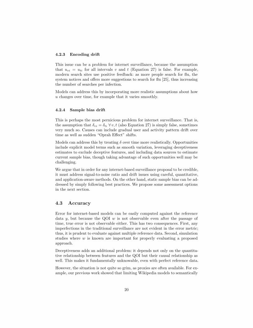
Figure 6: Alternatives to the deceptive feature in Figure 2 [6, 18]. These examplesshow that additional information can sometimes be used to reduce deceptiveness ininternet features. At top, expert knowledge about the patterns of seasonal flu is usedto identify and remove the deceptive period, replacing it with a linear interpolation.At bottom, Google’s proprietary machine learning algorithms are used to identify andcount searches likely related to the disease, rather than occurrences of a raw searchstring.

related articles reduced error [32]. Models can also reduce risk by monitoringcarefully for the breakdown in coincidental correlation that makes deceptive fea-tures troublesome. Our point is not that the situation is hopeless but that thateffective internet-based models must grapple quantitatively with deceptiveness.

We argue that doing so successfully is plausible; compare the features in Figure 6to the one in Figure 2. Properly designed internet-based surveillance might bealmost as accurate as traditional surveillance but available faster, providingsimilar value in a more nimble, and thus actionable, fashion.

21

5 Discussion

Traditional disease surveillance is not perfect. It has problems with static samplebias and, to a lesser degree, drifting bias. These are consequences of the fact thattraditional surveillance can only gather information from people in contact withthe health care system. Thus, expanding access to health care, outreach, andfurther work on compensating for these biases can improve incidence estimatesproduced by traditional surveillance.

Internet-based surveillance is not perfect either. In addition to inheriting most ofthe problems of traditional surveillance, with which it is necessarily entangled fortraining data, it adds signal-to-noise problems, further sample bias issues, andfurther drift as a consequence of its found encoder. Yet because it is inexpensiveand more timely, it holds great promise. So what is to be done? We proposethree things.

1. Because deceptiveness matters, model features should be selected that haveboth high correlation with reference data (to drive good predictions) andlow deceptiveness (to reduce the risk of including coincidentally predic-tive features). Existing data fitting techniques address the first part, andwe recommend adding a deceptiveness estimation step using additionalinformation such as semantic relatedness.

2. Because past model performance by itself is not predictive of future per-formance, model proposals should also include an analytical argumentsupporting their performance. One approach is to (a) define application-appropriate bounds on acceptable estimate error and deceptiveness, (b) de-rive the properties of input features necessary to meet those bounds, and(c) show that input features with those properties are available.

3. Because performance metrics include quantities unobservable in the realworld, no model should be evaluated only on real data. Models should alsobe evaluated on simulated disease outbreaks, which do not replicate thereal world in every detail but are valid tools for understanding [26], whereall quantities are known.

Internet-based disease surveillance cannot replace traditional surveillance, but itcan be an important complement because it is faster and cheaper with broaderreach. By better understanding the deficiencies of both along with their common-alities and relationship, using the tools proposed above, we can build quantitativearguments describing the added value of internet-based surveillance in specificsituations. Only then can it be relied on for life-and-death public health deci-sions [13].

22

Acknowlegements

This work was supported in part by the U.S. Department of Energy throughthe LANL/LDRD Program. A.C. was funded in part by the National ScienceFoundation under awards IIS-1526674 and IIS-1618244. Sara Y. Del Valle, JohnSzymanski, and Kyle Hickmann provided important feedback.

References

[1] Deborah Adams, Kathleen Fullerton, Ruth Jajosky, Pearl Sharp, Diana On-weh, Alan Schley, Willie Anderson, Amanda Faulkner, and Kiersten Kugeler.Summary of notifiable infectious diseases and conditions — United States,2013. MMWR, 62(53), October 2015. doi:10.15585/mmwr.mm6253a1.

[2] Joshua D. Angrist and Jorn-Steffen Pischke. Mostly harmless econometrics:An empiricist’s companion. 2009.

[3] Declan Butler. When Google got flu wrong. Nature, 494(7436), February2013. doi:10.1038/494155a.

[4] Centers for Disease Control and Prevention. MMWR morbidity tables.Dataset, 2015. URL: http://wonder.cdc.gov/mmwr/mmwrmorb.asp.

[5] Centers for Disease Control and Prevention. Overview of influenza surveil-lance in the United States. Fact sheet, October 2016. URL: https:

//www.cdc.gov/flu/pdf/weekly/overview-update.pdf.

[6] Centers for Disease Control and Prevention (CDC). FluView, 2017. URL:http://gis.cdc.gov/grasp/fluview/fluportaldashboard.html.

[7] Courtney D. Corley, Diane J. Cook, Armin R. Mikler, and Karan P. Singh.Text and structural data mining of influenza mentions in web and socialmedia. Environmental Research and Public Health, 7(2), February 2010.doi:10.3390/ijerph7020596.

[8] Aron Culotta. Lightweight methods to estimate influenza rates and alcoholsales volume from Twitter messages. Language Resources and Evaluation,47(1), March 2013. doi:10.1007/s10579-012-9185-0.

[9] Sunita Desai and Anupam B. Jena. Do celebrity endorsements matter?Observational study of BRCA gene testing and mastectomy rates afterAngelina Jolie’s New York Times editorial. BMJ, 355, December 2016.doi:10.1136/bmj.i6357.

[10] Maeve Duggan, Nicole B. Ellison, Cliff Lampe, Amanda Lenhart, and MaryMadden. Social media update 2014. Technical report, Pew ResearchCenter, January 2015. URL: http://www.pewinternet.org/2015/01/09/demographics-of-key-social-networking-platforms-2/.

23

[11] Flu Trends Team. The next chapter for Flu Trends, August2015. URL: http://googleresearch.blogspot.com/2015/08/the-next-chapter-for-flu-trends.html.

[12] Joao Gama, Indre Zliobaite, Albert Bifet, Mykola Pechenizkiy, and Abdel-hamid Bouchachia. A survey on concept drift adaptation. ACM ComputingSurveys, 46(4), March 2014. doi:10.1145/2523813.

[13] Nicholas Generous, Geoffrey Fairchild, Alina Deshpande, Sara Y. Del Valle,and Reid Priedhorsky. Global disease monitoring and forecasting withWikipedia. PLOS Computational Biology, 10(11), November 2014. doi:

10.1371/journal.pcbi.1003892.

[14] Edmund L. Gettier. Is justified true belief knowledge? Analysis, 23(6), June1963. URL: http://www.jstor.org/stable/3326922.

[15] Cheryl L Gibbons, Marie-Josee J Mangen, Dietrich Plass, Arie H Havelaar,Russell John Brooke, Piotr Kramarz, Karen L Peterson, Anke L Stuurman,Alessandro Cassini, Eric M Fevre, and Mirjam EE Kretzschmar. Measuringunderreporting and under-ascertainment in infectious disease datasets: Acomparison of methods. BMC Public Health, 14(1), December 2014. doi:

10.1186/1471-2458-14-147.

[16] Jeremy Ginsberg, Matthew H. Mohebbi, Rajan S. Patel, Lynnette Brammer,Mark S. Smolinski, and Larry Brilliant. Detecting influenza epidemicsusing search engine query data. Nature, 457(7232), November 2008. doi:

10.1038/nature07634.

[17] Google Inc. Search using autocomplete - Search Help, 2016. URL: https://support.google.com/websearch/answer/106230?hl=en.

[18] Google Inc. Google Trends, 2017. URL: https://trends.google.com/trends/.

[19] Nicholas M. Halzack and Thomas R. Miller. Patients cared for by theVeterans Health Administration present unique challenges to health careproviders. Policy brief Vol 2. Issue 3, American Society of Anesthesiologists,April 2014.

[20] Olga L. Henao, Timothy F. Jones, Duc J. Vugia, and Patricia M. Griffin.Foodborne diseases active surveillance network — 2 decades of achievements,1996–2015. Emerging Infectious Diseases, 21(9), September 2015. doi:

10.3201/eid2109.150581.

[21] Dorothy M. Horstmann. Importance of disease surveillance. PreventiveMedicine, 3(4), December 1974. doi:10.1016/0091-7435(74)90003-6.

[22] Ruth Ann Jajosky and Samuel L Groseclose. Evaluation of reporting time-liness of public health surveillance systems for infectious diseases. BMCPublic Health, 4(1), July 2004. doi:10.1186/1471-2458-4-29.

24

[23] L Jiang, V Lee, W Lim, M Chen, Y Chen, L Tan, R Lin, Y Leo, I Barr,and A Cook. Performance of case definitions for influenza surveillance.Eurosurveillance, 20(22), June 2015. doi:10.2807/1560-7917.ES2015.20.22.21145.

[24] Graham Kalton. Introduction to survey sampling, volume 07-035. 1983.

[25] David Lazer, Ryan Kennedy, Gary King, and Alessandro Vespignani. Theparable of Google Flu: Traps in big data analysis. Science, 343(6176), March2014. URL: http://science.sciencemag.org/content/343/6176/1203.

[26] Bruce Y. Lee, Virginia L. Bedford, Mark S. Roberts, and Kathleen M.Carley. Virtual epidemic in a virtual city: Simulating the spread of influenzain a US metropolitan area. Translational Research, 151(6), June 2008.doi:10.1016/j.trsl.2008.02.004.

[27] Nicole P. Lindsey, Jennifer A. Brown, Lon Kightlinger, Lauren Rosenberg,and Marc Fischer. State health department perceived utility of and satisfac-tion with ArboNET, the U.S. national arboviral surveillance system. PublicHealth Reports, 127(4), 2012. URL: http://www.ncbi.nlm.nih.gov/pmc/articles/PMC3366375/.

[28] Colin D. Mathers and Dejan Loncar. Projections of global mortality andburden of disease from 2002 to 2030. PLOS Medicine, 3(11), November2006. doi:10.1371/journal.pmed.0030442.

[29] National Center for Health Statistics. 2015 data release. Dataset, Jan-uary 2017. URL: https://www.cdc.gov/nchs/nhis/nhis_2015_data_

release.htm.

[30] Kenrad E. Nelson and Carolyn Williams. Infectious disease epidemiology.March 2013.

[31] Gordon L. Nichols, Yvonne Andersson, Elisabet Lindgren, Isabelle De-vaux, and Jan C. Semenza. European monitoring systems and datafor assessing environmental and climate impacts on human infectiousdiseases. Environmental Research and Public Health, 11(4), April 2014.doi:10.3390/ijerph110403894.

[32] Reid Priedhorsky, David A. Osthus, Ashlyn R. Daughton, Kelly Moran,Nicholas Generous, Geoffrey Fairchild, Alina Deshpande, and Sara Y.Del Valle. Measuring global disease with Wikipedia: Success, failure, and aresearch agenda. In Computer Supported Cooperative Work (CSCW), 2017.doi:10.1145/2998181.2998183.

[33] Rathergood. The internet is made of cats, January 2010. URL: https://www.youtube.com/watch?v=zi8VTeDHjcM.

[34] G.J. Rubin, H.W.W. Potts, and S. Michie. The impact of communicationsabout swine flu (influenza A H1N1v) on public responses to the outbreak:

25

Results from 36 national telephone surveys in the UK. Health TechnologyAssessment, 14(34), July 2010. doi:10.3310/hta14340-03.

[35] N. Savard, L. Bedard, R. Allard, and D. L. Buckeridge. Using age, triagescore, and disposition data from emergency department electronic records toimprove Influenza-like illness surveillance. Journal of the American MedicalInformatics Association, February 2015. doi:10.1093/jamia/ocu002.

[36] Jeffrey Shaman, Alicia Karspeck, Wan Yang, James Tamerius, and MarcLipsitch. Real-time influenza forecasts during the 2012–2013 season. NatureCommunications, 4(2387), December 2013. doi:10.1038/ncomms3837.

[37] Claude E. Shannon. A mathematical theory of communication. Bell Sys-tem Technical Journal, 27(3), July 1948. doi:10.1002/j.1538-7305.1948.tb01338.x.

[38] S. B. Thacker, R. G. Parrish, and F. L. Trowbridge. A method for evaluatingsystems of epidemiological surveillance. World Health Statistics Quarterly,41(1), 1988.

[39] User:Henrik. Wikipedia article traffic statistics, 2014. URL: http://stats.grok.se/.

[40] Benjamin Zablotsky, Lindsey I. Black, Matthew J. Maenner, Laura A.Schieve, and Stephen J. Blumberg. Estimated prevalence of autism andother developmental disabilities following questionnaire changes in the 2014National Health Interview survey. National Health Statistics Reports, 87,November 2015. URL: https://www.cdc.gov/nchs/data/nhsr/nhsr087.pdf.

[41] Erik Zachte. Wikipedia statistics all languages, November 2016. URL:https://stats.wikimedia.org/EN/TablesWikipediaZZ.htm.

26