Decentralized H controllerdesignforlarge …jerlynch/papers/HinfEESD.pdf · 378 Y. WANG, J. P....

EARTHQUAKE ENGINEERING AND STRUCTURAL DYNAMICSEarthquake Engng Struct. Dyn. 2009; 38:377–401Published online 19 November 2008 in Wiley InterScience (www.interscience.wiley.com). DOI: 10.1002/eqe.862

DecentralizedH∞ controller design for large-scale civil structures

Yang Wang1,∗,†, Jerome P. Lynch2 and Kincho H. Law3

1School of Civil and Environmental Engineering, Georgia Institute of Technology, Atlanta, GA 30332, U.S.A.2Department of Civil and Environmental Engineering, University of Michigan, Ann Arbor, MI 48109, U.S.A.

3Department of Civil and Environmental Engineering, Stanford University, Stanford, CA 94305, U.S.A.

SUMMARY

Complexities inherent to large-scale modern civil structures pose many challenges in the design of feedbackstructural control systems for dynamic response mitigation. With the emergence of low-cost sensors andcontrol devices creating technologies from which large-scale structural control systems can deploy, a futurecontrol system may contain hundreds, or even thousands, of such devices. Key issues in such large-scalestructural control systems include reduced system reliability, increasing communication requirements, andlonger latencies in the feedback loop. To effectively address these issues, decentralized control strategiesprovide promising solutions that allow control systems to operate at high nodal counts.

This paper examines the feasibility of designing a decentralized controller that minimizes the H∞norm of the closed-loop system. H∞ control is a natural choice for decentralization because impositionof decentralized architectures is easy to achieve when posing the controller design using linear matrixinequalities. Decentralized control solutions are investigated for both continuous-time and discrete-timeH∞ formulations. Numerical simulation results using a 3-story and a 20-story structure illustrate thefeasibility of the different decentralized control strategies. The results also demonstrate that when realisticsemi-active control devices are used in combination with the decentralized H∞ control solution, betterperformance can be gained over the passive control cases. It is shown that decentralized control strategiesmay provide equivalent or better control performance, given that their centralized counterparts could sufferfrom longer sampling periods due to communication and computation constraints. Copyright q 2008 JohnWiley & Sons, Ltd.

Received 19 June 2008; Revised 8 September 2008; Accepted 9 September 2008

KEY WORDS: H-infinity control; feedback structural control; decentralized control; smart structures

∗Correspondence to: Yang Wang, School of Civil and Environmental Engineering, Georgia Institute of Technology,Atlanta, GA 30332, U.S.A.

†E-mail: [email protected]

Contract/grant sponsor: Office of Naval ResearchContract/grant sponsor: Office of Technology Licensing Stanford Graduate FellowshipContract/grant sponsor: NSF; contract/grant number: CMMI-0824977

Copyright q 2008 John Wiley & Sons, Ltd.

378 Y. WANG, J. P. LYNCH AND K. H. LAW

1. INTRODUCTION

Real-time feedback control has been a topic of great interest to the structural engineering commu-nity over the last few decades [1–4]. A feedback structural control system includes an integratednetwork of sensors, controllers, and control devices that are installed in the civil structure to miti-gate undesired vibrations during external excitations, such as earthquakes or typhoons. Under anexternal excitation, the dynamic response of the structure is measured by sensors. Sensor data arecommunicated to a centralized controller that uses the data to calculate an optimal control solution.The optimal solution is then dispatched by the controller to control devices, which directly (i.e.active devices) or indirectly (i.e. semi-active devices) apply forces to the structure. This processrepeats continuously in real time to mitigate, or even eliminate, undesired structural vibrations. Itwas recently reported that more than 50 buildings and towers have been successfully instrumentedwith various types of structural control systems from 1989 to 2003 [5]. In practice, semi-activecontrol is usually preferred over active control because it can achieve at least an equivalent levelof performance, consumes orders of magnitude less power, and provides higher level of relia-bility. Examples of semi-active control devices include active variable stiffness devices, semi-activehydraulic dampers (SHD), electrorheological dampers, and magnetorheological dampers [6]. Addi-tional advantages associated with semi-active control include adaptability to real-time excitation,inherent bounded input/bounded output stability, and invulnerability against power failure.

Traditional feedback structural control systems employ centralized architectures. In such anarchitecture, one central controller is responsible for collecting data from all the sensors in thestructure, making control decisions, and dispatching these control decisions to control devices.Hence, the requirements on communication range and data transmission bandwidth increase withthe size of the structure and with the number of sensors and control devices being deployed. Thecommunication requirements could impose economical and technical difficulties for the implemen-tation of feedback control systems in increasingly larger civil structures. The centralized controlleritself represents a single point of potential failure; failure of the controller may paralyze the entirecontrol system. In order to overcome these inherent challenges, decentralized control architecturescould be alternatively adopted [7–9]. For example, a structural control system consisting of 88fully decentralized semi-active oil dampers has been installed in the 170m-tall Shiodome Towerin Tokyo, Japan [10, 11].

This paper examines both fully decentralized scheme, where the controller on a floor only haslocal sensor data from that floor, and partially decentralized scheme, where the controller alsoreceives sensor data from neighboring floors (or substructures). In a decentralized control systemarchitecture, multiple controllers are distributed throughout the structure. Acquiring data from alocal subnet of sensors, each controller commands control devices in its vicinity. The benefits oflocalizing a subset of sensors and control devices to each controller include shorter communicationranges and reduced data transmission rates in the control system. Decentralization also eliminatesthe risk of global control system failure if one of the controllers should fail. For large-scalestructures, occasional failure of decentralized controllers may only cause minor degradation to thecontrol performance.

Decentralized control design based on the linear quadratic regulator (LQR) optimization criteriahas been previously explored by the authors to study the feasibility of utilizing wireless sensors ascontrollers for feedback structural control [12, 13]. This paper investigates a different approach tothe design of a decentralized control system based on H∞ control theory, which is known to offerexcellent control performance when ‘worst-case’ external disturbances are encountered. Owing to

Copyright q 2008 John Wiley & Sons, Ltd. Earthquake Engng Struct. Dyn. 2009; 38:377–401DOI: 10.1002/eqe

DECENTRALIZED H∞ CONTROLLER DESIGN 379

the multiplicative property of the H∞ norm [14], H∞ control design can also consider modelinguncertainties (as is typical in most civil structures). Centralized H∞ controller implementationin the continuous-time domain for civil structural control has been extensively studied [15–21].When compared with traditional linear quadratic Gaussian controllers,H∞ controllers can achieveeither comparable or superior performance [22, 23]. For example, it has been shown that H∞control design may achieve better performance in attenuating transient vibrations of the structure[24]. However, decentralized H∞ controller design, either in the continuous-time domain ordiscrete-time domain, has rarely been explored in structural control.

TheH∞ control solution can be readily formulated as an optimization problem with constraintsexpressed in terms of linear matrix inequalities (LMI) [25]. For such problems, sparsity patternscan be easily applied to the controller matrix variables. This property offers significant conveniencefor designing decentralized controllers, where certain sparsity patterns can be applied to the gainmatrices consistent with certain desired feedback architecture. This paper presents pilot studiesinvestigating the feasibility of decentralized H∞ control that may be employed in large-scalestructural control systems. More specifically, decentralized H∞ controller design is presented inboth the continuous-time and discrete-time domains. Using properties of LMI, the decentralizedH∞ control problem is converted into a convex optimization problem that can be convenientlysolved using available mathematical packages.

Numerical simulations are conducted to validate the performance of the decentralized H∞controller design. In the first example, a 3-story structure is used to demonstrate the detailed proce-dure for the design of the decentralized H∞ controller. The control performance of decentralizedH∞ controllers is then compared with the performance of decentralized LQR-based controllers[12, 13]. In the second example, simulations of a 20-story benchmark structure are conducted toillustrate the efficacy of the decentralized H∞ control solution for large-scale civil structures.Different information feedback architectures and control sampling rates are employed so as toprovide an in-depth study of the proposed approaches. Control performance using ideal actuatorsand large-capacity SHD dampers are presented for the 20-story structure. Performance of thedecentralized control system is compared with passive control cases where the SHD dampers arefixed at minimum or maximum damping settings.

2. FORMULATION OF DECENTRALIZED H∞ CONTROL

This section first discusses the design of a decentralizedH∞ controller for structural control in thecontinuous-time domain. The controller’s counterpart in the discrete-time domain is then derived.In both derivations, properties of LMI are utilized to convert the formulation of the decentralizedcontrol design problem into a convex optimization problem.

2.1. Continuous-time decentralized H∞ control

For a lumped-mass structural model with n degrees-of-freedom subjected tom1 external excitations,and controlled by m2 control devices, the equations of motion can be formulated as

Mq(t)+Cq(t)+Kq(t)=Tuu(t)+Tww(t) (1)

where q(t)∈Rn×1 is the displacement vector relative to the ground; M, C, K∈Rn×n are the mass,damping, and stiffness matrices, respectively; u(t)∈Rm2×1 and w(t)∈Rm1×1 are the control force



Figure 1. A three-story controlled structure excited by unidirectional ground motion.

and external excitation vectors, respectively; and Tu∈Rn×m2 and Tw∈Rn×m1 are the control andexcitation location matrices, respectively.

For simplicity, the discussion is based on a 2D shear–frame structure subjected to unidirectionalground excitation. In the example structure shown in Figure 1, it is assumed that the externalexcitation, w(t), is a scalar function (m1=1) containing the ground acceleration time history qg(t);the spatial load pattern Tw is then equal to −M{1}n×1. Entries in u(t) are defined as the controlforces between neighboring floors. For the 3-story structure, if a positive control force is definedto be moving the floor above the device toward the left direction, and moving the floor below thedevice toward the right direction (as shown in Figure 1), the control force location matrix Tu isdefined as

Tu=⎡⎢⎣

−1 1 0

0 −1 1

0 0 −1

⎤⎥⎦ (2)

The second-order ordinary differential equation (ODE), Equation (1), can be converted to a first-order ODE by the state-space formulation as follows:

xI(t)=AIxI(t)+BIu(t)+EIw(t) (3)

where xI=[q(t); q(t)]∈R2n×1 is the state vector; AI∈R2n×2n , BI∈R2n×m2 , and EI∈R2n×m1 arethe system, control, and excitation matrices, respectively:

AI=[ [0]n×n [I]n×n

−M−1K −M−1C

], BI=

[[0]n×m2

M−1Tu

], EI=

[ {0}n×1

−{1}n×1

](4)

In this study, it is assumed that inter-story drifts and velocities are measurable. The displacementand velocity variables in xI, which are relative to the ground, are first transformed into inter-storydrifts and velocities (i.e. drifts and velocities between neighboring floors). The inter-story driftsand velocities at each story are then grouped together as:

x=[q1 q1 q2 −q1 q2− q1, . . . ,qn−qn−1 qn− qn−1]T (5)



A linear transformation matrix C∈R2n×2n can be defined such that x=CxI. Substituting xI=C−1xinto Equation (3), and left multiplying the equation with C, the state-space representation with thetransformed (inter-story) state vector becomes

x(t)=Ax(t)+Bu(t)+Ew(t) (6)

where

A=CAIC−1, B=CBI, E=CEI (7)

The system output z(t)∈Rp×1 is defined as the sum of linear transformations to the state vectorx(t) and the control force vector u(t):

z(t)=Czx(t)+Dzu(t) (8)

where Cz∈Rp×2n and Dz∈Rp×m2 are the output matrices for the state and control force vectors,respectively. Assuming static state feedback, the control force u(t) is determined by u(t)=Gx(t),where G∈Rm2×2n is termed the control gain matrix. Substituting Gx(t) for u(t) in Equations (6)and (8), the state-space equations of the closed-loop system can be written as:

x(t) = ACLx(t)+Ew(t)

z(t) = CCLx(t)(9)

where

ACL = A+BG

CCL = Cz+DzG(10)

In frequency domain, the system dynamics can be represented by the transfer function Hzw(s)∈Cp×m1 from disturbance w(t) to output z(t) as [26]

Hzw(s)=CCL(sI−ACL)−1E (11)

where s is the complex Laplacian variable. The objective of H∞ control is to minimize theH∞-norm of the closed-loop system, which in the frequency domain is defined as

‖Hzw(s)‖∞ =sup�

�[Hzw( j�)] (12)

where � represents angular frequency, j is the imaginary unit, �[·] denotes the largest singularvalue of a matrix, and ‘sup’ denotes the supremum (least upper bound) of a set of real numbers.The definition shows that in the frequency domain, the H∞-norm of the system is equal to thepeak of the largest singular value of the transfer function Hzw(s) along the imaginary axis (wheres= j�). The H∞-norm also has an equivalent interpretation in the time domain, as the supremumof the 2-norm amplification from the disturbance to the output:

‖Hzw(s)‖∞ = supw,‖w(t)‖2 �=0

(‖z(t)‖2/‖w(t)‖2) (13)

where the 2-norm of a signal f(t) is defined as ‖f(t)‖2=√∫ t=+∞

t=−∞ fT(t)f(t)dt , which representsthe energy level of a signal. In this study, the H∞-norm can be viewed as the upper limit of



the amplification factor from the disturbance (i.e. seismic ground motion) energy to the output(i.e. structural response) energy. The disturbance is called a ‘worst-case’ disturbance when thisupper limit is reached. By minimizing the H∞-norm, the system output (which includes structuralresponse measures) can be greatly reduced when a worst-case disturbance (which is the earthquakeexcitation) is applied.

According to the Bounded Real Lemma, the following two statements are equivalent for aH∞ controller that minimizes the smallest upper bound of the H∞-norm of a continuous-timesystem [25]:

1. ‖Hzw‖∞ <� and ACL is stable in the continuous-time sense (i.e. the real parts of all theeigenvalues of ACL are negative).

2. There exists a symmetric positive-definite matrix H∈R2n×2n such that the followinginequality holds: [

ACLH+HATCL+EET/�2 HCT

CL

∗ −I

]<0 (14)

where ∗ denotes the symmetric entry (in this case, CCLH), and ‘<0’ means that the matrixat the left side of the inequality is negative definite. Using the closed-loop matrix definitionsin Equation (10), Equation (14) becomes[

AH+HAT+BGH+HGTBT+EET/�2 HCTz +HGTDT

z

∗ −I

]<0 (15)

The above nonlinear matrix inequality can be converted into LMI by introducing a new variableY∈Rm2×2n where Y=GH[

AH+HAT+BY+YTBT+EET/�2 HCTz +YTDT

z

∗ −I

]<0 (16)

In summary, the continuous-time H∞ control problem is now transformed into a convexoptimization problem:

minimize �

subject to H>0 and the LMI expressed in Equation (16)(17)

Here Y, H, and � are the optimization variables. Numerical solutions to this optimization problemcan be computed, for example, using the Matlab LMI Toolbox [27] or the convex optimizationpackage CVX [28]. After the optimization problem is solved, the control gain matrix is computed as:

G=YH−1 (18)

In general, the algorithm finds a gain matrix without any sparsity constraints; in other words,it represents a control scheme consistent with a centralized state feedback architecture. Tocompute gain matrices for decentralized state feedback control, appropriate sparsity constraintscan be applied to the optimization variables Y and H while solving the optimization problem of



Equation (17). For most available software packages, the sparsity constraints can be convenientlydefined by assigning corresponding zero entries to the Y and H optimization variables. Forexample, gain matrices of the following sparsity patterns may be employed for a three-storystructure:

GI=⎡⎢⎣

� 0 0

0 � 0

0 0 �

⎤⎥⎦ and GII=

⎡⎢⎣

� � 0

� � �0 � �

⎤⎥⎦ (19)

Note that each entry in the above matrices represents a 1×2 block. According to the linearfeedback control law u(t)=Gx(t), when the sparsity pattern in GI is used, only the inter-storydrift and velocity at the i th story are needed to determine the control force ui at the same story.When the sparsity pattern in GII is adopted, the inter-story drifts and velocities from both the i thstory and the neighboring stories (story) are needed in order to determine the control force uiat the i th story. Considering the relationship between G and Y as specified in Equation (18), inorder to find the control gain matrices satisfying the shape constraints in GI, the following shapeconstraints may be applied to the optimization variables Y and H:

YI=⎡⎢⎣

� 0 0

0 � 0

0 0 �

⎤⎥⎦ and HI=

⎡⎢⎣

� 0 0

0 � 0

0 0 �

⎤⎥⎦ (20)

Similarly, to compute control gain matrices satisfying the shape constraints of GII, the followingshape constraints may be applied to the optimization variables:

YII=⎡⎢⎣

� � 0

� � �0 � �

⎤⎥⎦ and HII=

⎡⎢⎣

� 0 0

0 � 0

0 0 �

⎤⎥⎦ (21)

It is important to realize that due to the constraints imposed on the Y and H variables, thepresented decentralized H∞ controller precludes the possibility that a decentralized gain matrixmay exist with Y and H variables not satisfying the corresponding shape constraints. For example,it is possible that a gain matrix may satisfy the sparsity pattern in GI while the corresponding Yand H variables do not conform to the sparsity patterns shown in Equation (20). The applicationof sparsity patterns to Y and H variables makes the gain matrix easily computable using existingsoftware packages, although the approach may not be able to explore the complete solution spaceof decentralized gain matrices. That is, the approach for decentralized H∞ controller design maynot guarantee that a minimumH∞-norm is obtained over the complete solution space; rather, onlya minimum H∞-norm is obtained for the solution space contained within the boundary imposedby the shape constraints on Y and H.



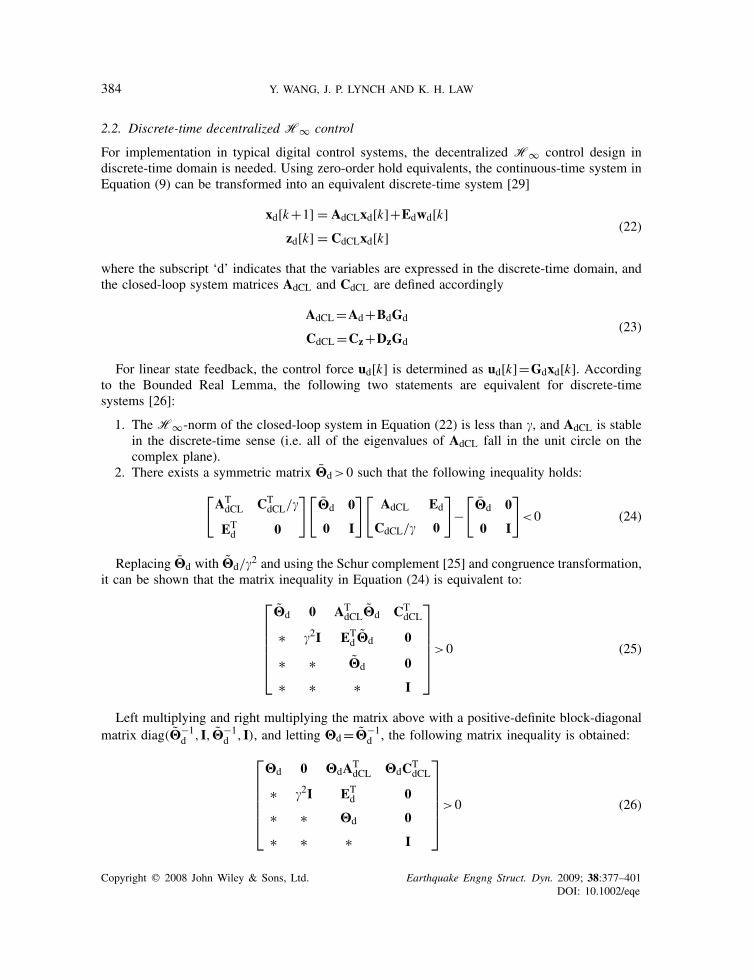
2.2. Discrete-time decentralized H∞ control

For implementation in typical digital control systems, the decentralized H∞ control design indiscrete-time domain is needed. Using zero-order hold equivalents, the continuous-time system inEquation (9) can be transformed into an equivalent discrete-time system [29]

xd[k+1] = AdCLxd[k]+Edwd[k]zd[k] = CdCLxd[k]

(22)

where the subscript ‘d’ indicates that the variables are expressed in the discrete-time domain, andthe closed-loop system matrices AdCL and CdCL are defined accordingly

AdCL=Ad+BdGd

CdCL=Cz+DzGd(23)

For linear state feedback, the control force ud[k] is determined as ud[k]=Gdxd[k]. Accordingto the Bounded Real Lemma, the following two statements are equivalent for discrete-timesystems [26]:

1. The H∞-norm of the closed-loop system in Equation (22) is less than �, and AdCL is stablein the discrete-time sense (i.e. all of the eigenvalues of AdCL fall in the unit circle on thecomplex plane).

2. There exists a symmetric matrix Hd>0 such that the following inequality holds:

[ATdCL CT

dCL/�

ETd 0

][Hd 0

0 I

][AdCL Ed

CdCL/� 0

]−

[Hd 0

0 I

]<0 (24)

Replacing Hd with Hd/�2 and using the Schur complement [25] and congruence transformation,it can be shown that the matrix inequality in Equation (24) is equivalent to:

⎡⎢⎢⎢⎢⎢⎣

Hd 0 ATdCLHd CT

dCL

∗ �2I ETd Hd 0

∗ ∗ Hd 0

∗ ∗ ∗ I

⎤⎥⎥⎥⎥⎥⎦>0 (25)

Left multiplying and right multiplying the matrix above with a positive-definite block-diagonalmatrix diag(H−1

d ,I,H−1d ,I), and letting Hd=H−1

d , the following matrix inequality is obtained:

⎡⎢⎢⎢⎢⎢⎣

Hd 0 HdATdCL HdCT

dCL

∗ �2I ETd 0

∗ ∗ Hd 0

∗ ∗ ∗ I

⎤⎥⎥⎥⎥⎥⎦>0 (26)



Similar to the continuous-time system, by replacing the closed-loop matrices AdCL and CdCLin Equation (26) with their definitions in Equation (23), and letting Yd=GdHd, the above matrixinequality can be converted into:

⎡⎢⎢⎢⎢⎢⎣

Hd 0 HdATd +YT

dBTd HdCT

z +YTdD

Tz

∗ �2I ETd 0

∗ ∗ Hd 0

∗ ∗ ∗ I

⎤⎥⎥⎥⎥⎥⎦>0 (27)

Therefore, the discrete-time H∞ control problem can be converted to a convex optimizationproblem with LMI constraints:

minimize �

subject to Hd>0 and the LMI expressed in Equation (27)(28)

Here again, Yd, Hd, and � are the optimization variables. After the optimization problem is solved,the control gain matrix is computed as:

Gd=YdH−1d (29)

Furthermore, the sparsity pattern of the gain matrix can be obtained by specifying appropriatezero entries to the LMI variables Yd and Hd, following the same procedure as described in thecontinuous-time case.

3. NUMERICAL SIMULATIONS

Since the discrete-time formulation is suitable for implementation in modern digital controllers,numerical simulations are conducted to evaluate the performance of the discrete time decentralizedH∞ control schemes described in Section 2.2. In Section 3.1, the procedure for designing thedecentralized H∞ controller is illustrated in details using a 3-story structure. Performance of theH∞ controllers is compared with the performance of controllers based on the LQR optimizationcriteria. In Section 3.2, simulations using a 20-story benchmark structure are conducted to illustratethe efficacy of the decentralized H∞ control solution for large-scale civil structures. Results usingboth ideal actuators and large-capacity SHD dampers are presented for the 20-story structure.

3.1. Numerical simulation of a 3-story structure

3.1.1. Decentralized H∞ control. Simulations of a 3-story shear–frame structure are firstpresented to illustrate the procedure employed in decentralized H∞ control design. The framestructure is modeled as an in-plane lumped-mass shear structure with one actuator allocatedbetween every two neighboring floors. It is assumed that both the inter-story drifts and inter-storyvelocities between every two neighboring floors are measurable. Such an assumption is reasonable



considering that modern SHD dampers contain internal stroke sensors and load cells that measurereal-time damper displacements and forces, respectively [11]. Assuming V-brace elements areused as shown in Figure 1, the displacement and force measurements can be used to estimateinter-story drifts and velocities. The following mass, stiffness, and damping matrices are adoptedfor the example structure:

M =

⎡⎢⎢⎣6

6

6

⎤⎥⎥⎦×103 kg, K=

⎡⎢⎢⎣

3.4 −1.8

−1.8 3.4 −1.6

−1.6 1.6

⎤⎥⎥⎦×106N/m

C =

⎡⎢⎢⎣

12.4 −5.16

−5.16 12.4 −4.59

−4.59 7.20

⎤⎥⎥⎦×103N/(m/s)

(30)

For unidirectional ground excitation, the continuous-time system matrices A, B, and E can beobtained via Equation (7) as

A =

⎡⎢⎢⎢⎢⎢⎢⎢⎢⎢⎢⎢⎢⎣

0 1 0 0 0 0

−266.7 −1.2 300 0.8603 0 0

0 0 0 1 0 0

266.7 0.7647 −600 −2.156 266.7 0.7647

0 0 0 0 0 1

0 0 300 0.8603 −533.3 −1.965

⎤⎥⎥⎥⎥⎥⎥⎥⎥⎥⎥⎥⎥⎦

B =

⎡⎢⎢⎢⎢⎢⎢⎢⎢⎢⎢⎢⎢⎣

0 0 0

−1.667 1.667 0

0 0 0

1.667 −3.333 1.667

0 0 0

0 1.667 −3.333

⎤⎥⎥⎥⎥⎥⎥⎥⎥⎥⎥⎥⎥⎦

×10−4, E=

⎡⎢⎢⎢⎢⎢⎢⎢⎢⎢⎢⎢⎣

0

−1

0

0

0

0

⎤⎥⎥⎥⎥⎥⎥⎥⎥⎥⎥⎥⎦

(31)

Note that the state-space vector corresponding to these matrices no longer contains displacementsand velocities relative to the ground. Instead, the vector has been formulated to contain inter-storydrifts and velocities that are grouped by floors as given in Equation (5). The system matrices in



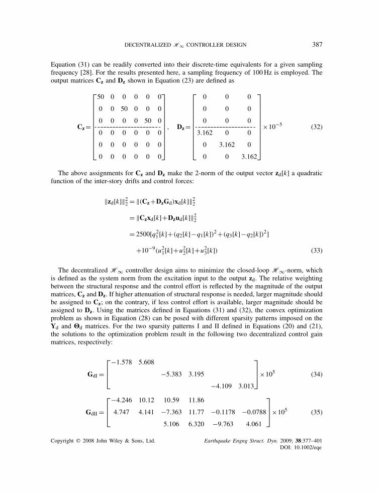
Equation (31) can be readily converted into their discrete-time equivalents for a given samplingfrequency [28]. For the results presented here, a sampling frequency of 100Hz is employed. Theoutput matrices Cz and Dz shown in Equation (23) are defined as

Cz=

⎡⎢⎢⎢⎢⎢⎢⎢⎢⎢⎢⎣

50 0 0 0 0 0

0 0 50 0 0 0

0 0 0 0 50 0- - -- - -- - -- - -- - -- - -- - -- - -- - -- - -- - -- - -- - -- - -- - -- - -- - -- - -- - -- - -0 0 0 0 0 0

0 0 0 0 0 0

0 0 0 0 0 0

⎤⎥⎥⎥⎥⎥⎥⎥⎥⎥⎥⎦

, Dz=

⎡⎢⎢⎢⎢⎢⎢⎢⎢⎢⎢⎣

0 0 0

0 0 0

0 0 0- - -- - -- - -- - -- - -- - -- - -- - -- - -- - -- - -- - -- - -- - -- - -- - -- - -- - -3.162 0 0

0 3.162 0

0 0 3.162

⎤⎥⎥⎥⎥⎥⎥⎥⎥⎥⎥⎦

×10−5 (32)

The above assignments for Cz and Dz make the 2-norm of the output vector zd[k] a quadraticfunction of the inter-story drifts and control forces:

‖zd[k]‖22 = ‖(Cz+DzGd)xd[k]‖22= ‖Czxd[k]+Dzud[k]‖22= 2500[q21 [k]+(q2[k]−q1[k])2+(q3[k]−q2[k])2]

+10−9(u21[k]+u22[k]+u23[k]) (33)

The decentralized H∞ controller design aims to minimize the closed-loop H∞-norm, whichis defined as the system norm from the excitation input to the output zd. The relative weightingbetween the structural response and the control effort is reflected by the magnitude of the outputmatrices, Cz and Dz. If higher attenuation of structural response is needed, larger magnitude shouldbe assigned to Cz; on the contrary, if less control effort is available, larger magnitude should beassigned to Dz. Using the matrices defined in Equations (31) and (32), the convex optimizationproblem as shown in Equation (28) can be posed with different sparsity patterns imposed on theYd and Hd matrices. For the two sparsity patterns I and II defined in Equations (20) and (21),the solutions to the optimization problem result in the following two decentralized control gainmatrices, respectively:

GdI =⎡⎢⎣

−1.578 5.608

−5.383 3.195

−4.109 3.013

⎤⎥⎦×105 (34)

GdII =⎡⎢⎣

−4.246 10.12 10.59 11.86

4.747 4.141 −7.363 11.77 −0.1178 −0.0788

5.106 6.320 −9.763 4.061

⎤⎥⎦×105 (35)



Table I. H2- and H∞-norms of the open-loop transfer function Hzw and the closed-loop norms usingboth the H∞ controllers and LQR controllers.

Closed-loop

Fully decentralized Partially decentralized CentralizedOpen-loop

(Uncontrolled) GLQRdI GdI(H∞) GLQR

dII GdII(H∞) GLQRdIII GdIII(H∞)

H∞-norm 8.4366 1.2836 0.8521 1.0462 0.7076 0.9922 0.7045H2-norm 0.4657 0.1874 0.3020 0.1786 0.5027 0.1772 0.6108

When no sparsity pattern is applied to Yd and Hd, a full gain matrix representing centralizedfeedback is generated

GdIII=⎡⎢⎣

2.354 15.24 −0.6553 11.52 1.505 6.281

−3.719 10.04 3.358 8.539 1.125 4.499

−3.954 5.742 −1.599 4.726 5.687 3.269

⎤⎥⎦×105 (36)

The open-loop H∞-norm of the uncontrolled structure and the closed-loop H∞-norms ofthe controlled structure using the above gain matrices are listed in Table I. The H∞-norm of theuncontrolled structure is computed using the discrete-time system defined in Equation (22) with thegain matrix Gd set as a zero matrix. Comparing the four cases in Table I, the uncontrolled structurehas the highestH∞-norm (8.4366), which indicates the largest ‘worst-case’ amplification from theexcitation input wd to the output zd. Among the three controlled cases, because the centralized casewith gain matrix GdIII assumes that complete state information is available for control decisions,the lowest H∞-norm (0.7045) is achieved (which means best control performance). The fullydecentralized case with gain matrix GdI has the largest norm (0.8521) among the three H∞controllers; this is somewhat expected because the fully decentralized controller has the leastamount of information available for calculating control decisions for each control device.

The 1940 El Centro NS (Imperial Valley Irrigation District Station) earthquake record with itspeak acceleration scaled to 1m/s2 is used as the ground excitation. Three ideal actuators thatgenerate any desired control force are deployed at the three stories. In contrast to a realistic semi-active or active control device, an ideal actuator offers unlimited force capacity, and has zero timedelay while delivering the force. Maximum inter-story drifts and control forces during the dynamicresponse are plotted in Figure 2. The inter-story drift plots in Figure 2(a) include the results for theuncontrolled structure and the structure controlled using the three different gain matrices. Usingideal actuators, all three controlled cases achieve significant reduction in inter-story drifts comparedwith the uncontrolled case. Among the three controlled cases, the fully decentralized case usinggain matrix GdI achieves the smallest reduction in inter-story drifts, which is consistent with theperformance comparison indicated by the H∞-norms in Table I. The difference between the casesusing gain matrices GdII and GdIII is minor, with GdIII achieving slightly better performance.

Figure 2(b) presents the peak control forces for the three controlled cases. The fully decentralizedcontroller imposes the lowest requirements on the control force capacity. The peak control forcesare similar between the partially decentralized case GdII and the centralized case GdIII. The largestsum of the three peak actuator forces is about 35 kN, which represents the total capacity of all the



Figure 2. Simulation results when ideal actuators are deployed on the 3-story structure.

Table II. RMS values of control forces and the changes in RMS inter-story drifts (H∞ control cases).

Controlled

RMS of GdI GdII GdIIIuncontrolledinter-story Drift Force Drift Force Drift Forcedrift (mm) change (%) (kN) change (%) (kN) change (%) (kN)

Story-1 2.9 −85 2.06 −95 3.08 −96 3.09Story-2 2.1 −78 1.35 −95 2.08 −96 2.06Story-3 1.4 −82 0.69 −95 1.05 −94 1.09Average N/A −82 1.37 −95 2.07 −95 2.08

actuators. This amount of total actuator capacity is about 19% of the building weight (180 kN), arealistic ratio as suggested by most references [30–32].

Further illustration of the trade-off between structural response attenuation and control effortis shown in Table II. The table first lists the root-of-mean-square (RMS) values of the inter-storydrifts at all three floors when the structure is uncontrolled, i.e. 2.9, 2.1, and 1.4mm, respectively.For the three controlled cases, changes in RMS drifts are listed in percentages relative to theuncontrolled values, i.e. negative numbers represent reduction from the uncontrolled value. Forexample, case GdIII offers 96% reduction to the RMS drift at the first story. RMS values of threeactuator forces are also listed for the three controlled cases. For each controlled case, the bottomrow of Table II provides average drift changes and RMS forces across the three stories. It is againshown that cases GdII and GdIII offer greater reduction to structural response through larger controleffort.

3.1.2. Comparison with decentralized LQR control. It could be instructive to compare the decen-tralized H∞ controller design with the decentralized LQR controller design that was previouslystudied [12]. The LQR control algorithm aims to select the optimal control force trajectory ud by



minimizing the expected value of a quadratic cost function, J :

J =∞∑k=1

(xTd [k]Qxd[k]+uTd [k]Rud[k]), Q2n×2n�0 and Rm2×m2 >0 (37)

Using the same definition of the output matrices as described in Equation (32), the followingweighting matrices are employed for the LQR controller design:

Q=CTz Cz (38)

R=DTz Dz (39)

As a result, the LQR optimization index J is proportional to the signal 2-norm of the systemoutput:

J =K∑

k=1(xTd [k]CT

z Czxd[k]+uTd [k]DTz Dzud[k])

=K∑

k=1‖Czxd[k]+Dzud[k]‖22

=K∑

k=1‖zd[k]‖22

= ‖zd‖22/�t (40)

where �t is the sampling period, and note that CTz Dz=0 and DT

z Cz=0 using the definitions inEquation (32). The design of the LQR controller iteratively searches for an optimal control gainmatrix by traversing along the optimization gradient. Sparsity shape constraints are iterativelyapplied to the search gradient in order to compute the decentralized gain matrices. The followingthree decentralized/centralized LQR gain matrices are obtained:

GLQRdI =

⎡⎢⎣4.4137 1.2649

4.6383 0.9489

5.1068 0.6965

⎤⎥⎦×105 (41)

GLQRdII =

⎡⎢⎣5.4594 1.2150 −0.3170 0.4404

0.5689 0.5262 4.0575 0.8687 0.2693 0.2932

−0.1671 0.2163 5.0089 0.6818

⎤⎥⎦×105 (42)

GLQRdIII =

⎡⎢⎣5.2399 1.2321 0.8256 0.5676 0.1599 0.2438

0.5157 0.5230 4.1441 0.8631 0.4141 0.2975

0.1322 0.2427 0.6449 0.3228 4.5696 0.6714

⎤⎥⎦×105 (43)

Table I also lists the H2- and H∞-norms of the open-loop transfer function Hzw and theclosed-loop norms using both the H∞ controllers and the LQR controllers. Since the LQR control



Figure 3. Singular values of the closed-loop system transfer function Hzw( j�) using the decentralizedH∞ controller GdI and decentralized LQR controller GLQR

dI .

approach is equivalent to an H2 control design that minimizes the closed-loop H2-norm, LQRcontrollers are expected to perform well in reducing the closed-loop H2-norm [14, 33]. Similarto the H∞-norm, definition of the system H2-norm can also be written in terms of the singularvalues of the transfer function matrix:

‖Hzw(s)‖2=√

1

2�

∫ +∞

−∞∑i

�2i [Hzw( j�)]d� (44)

As expected, Table I shows that the LQR controllers, no matter decentralized or centralized,consistently perform better than their H∞ counterparts in reducing the H2-norm, while theH∞ controllers consistently perform better than their LQR counterparts in terms of reducing theH∞-norm.

In this example, the second dimension of the transfer function matrix Hzw( j�) is one, becausethe disturbance w is a scalar that represents the ground excitation. Therefore, Hzw( j�) has onlyone singular value at each frequency �, which is the largest singular value. Figure 3 plots thesingular value of the closed-loop system transfer function Hzw( j�) using the decentralized H∞controller GdI and the decentralized LQR controller GLQR

dI . The definition of the systemH∞-normin Equation (12) shows that the H∞-norm should be equal to the peak of the largest singular valueover the frequency span. Correspondingly, Figure 3 shows that the peak of the singular value usingthe H∞ controller GdI is about 0.85, while the peak for the LQR controller GLQR

dI is about 1.28;both of which are consistent with the H∞-norms listed in Table I. Figure 3 also illustrates thatthe decentralized H∞ controller excels at ‘pushing down the peak of the largest singular value.’In comparison, the decentralized LQR controller is shown to excel in reducing all singular valuesover the entire frequency span, which agrees with the objective of minimizing the H2-norm (asdefined in Equation (44)).

Simulations are conducted using the LQR controllers, with the same 1940 El Centro NS earth-quake excitation scaled to 1m/s2. Three ideal actuators are again deployed at the three stories.Maximum inter-story drifts and control forces during the dynamic response are plotted in Figure 4.



Figure 4. Simulation results when ideal actuators are deployed on the 3-story structure.

Comparison between Figures 2 and 4 show that LQR controllers generally achieve less reductionto peak inter-story drifts. On the other hand, the advantage of the LQR controllers in this exampleis that they impose lower requirements to the force capacity of the structural control devices. Forthe LQR control cases, the total actuator capacity is approximately 20 kN, i.e. about 11% of thebuilding weight. This ratio is much lower than the ratio of 19% for the H∞ control cases.

Similar to Table II for the H∞ control cases, further illustration of the trade-off betweenstructural response attenuation and control effort is shown in Table III for LQR control. For thecontrolled cases, changes in RMS drifts are again listed in percentages relative to the uncontrolledvalues. The table shows that as compared with case GLQR

dI , cases GLQRdII and GLQR

dIII offer greaterreduction to structural response at the expense of larger control effort. Comparing the bottom rowsof Tables II and III, it is again illustrated that the LQR cases achieve less attenuation to structuralresponse, while demanding less control effort.

3.2. Numerical simulation of a 20-story benchmark structure

3.2.1. Simulation using ideal actuators. To explore the performance of decentralized H∞ controlfor a larger-scale structure, a 20-story benchmark building designed for the Structural EngineersAssociation of California (SAC) project is selected [34]. Same as the 3-story example, discrete-timecontrollers are adopted in the simulation. The building is modeled as an in-plane lumped-massshear structure with control devices allocated between every set of neighboring floors. Figure 5(a)shows the mass, stiffness, and damping parameters of the structure. In the numerical simulations, itis assumed that both the inter-story drifts and inter-story velocities between every two neighboringfloors are measurable. As shown in Equation (5), the state-space equations are formulated suchthat the state-space vector contains inter-story drifts and velocities. Simulations are conductedfor different decentralization schemes as shown in Figure 5(b). The degree-of-centralization (DC)reflects the different communication architectures, with each communication subnet (as denoted bychannels Ch1, Ch2, etc.) covering a limited number of stories. The controllers covered by a subnetare allowed to access the sensor data within that subnet. For example, the case where DC=1has each subnet covering only five stories with a total of four subnets utilized. For DC=2, each



Table III. RMS values of control forces and the changes in RMS inter-story drifts (LQR control cases).

Controlled

RMS of GLQRdI GLQR

dII GLQRdIII

uncontrolledinter-story Drift Force Drift Force Drift Forcedrift (mm) change (%) (kN) change (%) (kN) change (%) (kN)

Story-1 2.9 −66 1.20 −71 1.32 −73 1.42Story-2 2.1 −65 0.76 −71 1.04 −72 1.01Story-3 1.4 −67 0.42 −72 0.46 −75 0.59Average N/A −66 0.79 −71 0.94 −73 1.01

Figure 5. Twenty-story SAC building for numerical simulations: (a) model parameters of the lumped-massstructure and (b) communication subnet partitioning for different degrees-of-centralization (DC).

subnet covers 10 stories and a total of three subnets are utilized; meanwhile, overlaps exist betweensubnets for DC=2. For stories covered by multiple overlapping subnets, each controller at thesestories should have communication access to data within all the overlapping subnets. Althougheach controller may command multiple control devices, in this example, a control device can onlybe commanded by one controller. The gain matrices for the decentralized information structureswith DC=1 and 2 have the following sparsity patterns:

when DC = 1; when DC = 2 (45)

Each entry in the above matrices represents a 5× 10 block submatrix. To achieve the sparsitypatterns in gain matrix Gd, the matrix variable Yd in Equation (28) is defined to have the samesparsity pattern as Gd, and Hd is defined to be always block-diagonal. For the cases where DC=3and 4, the number of stories covered by each communication subnet increases accordingly, whichresult in fewer zero blocks in Gd. Clearly, the case where DC=4 corresponds to a centralizedfeedback structure with all devices in the same subnet (i.e. Ch1).



To investigate the effectiveness of the proposed decentralized control design, we first assume the20-story structure is instrumented with ideal actuators that can produce any desired force. Outputmatrices Cz and Dz in Equation (23) are defined as

Cz=[102I40×40

020×40

], Dz=

[040×20

10−12I20×20

](46)

Simulations are performed for different DCs (DC=1, . . . ,4) and sampling periods (rangingfrom 0.01 to 0.06 s at a resolution of 0.01 s). Additionally, three ground motion records all scaledto a peak ground acceleration (PGA) of 1m/s2 are used for the simulation: 1940 El Centro NS(Imperial Valley Irrigation District Station), 1995 Kobe NS (JMA Station), and 1999 Chi-Chi NS(TCU-076 Station). Two representative performance indices, J1 and J2, as proposed by Spenceret al. [34] are adopted:

J1 = maxEarthquakes

{maxk,i

di [k]/

maxk,i

di [k]}

(47)

J2 = maxEarthquakes

{‖zd‖22/‖zd‖22} (48)

Here J1 and J2 correspond to maximum inter-story drifts and output vector zd, respectively. InEquation (47), di [k] represents the inter-story drift between floor i (i=1, . . . ,n) and its lowerfloor at time step k, and maxk,i di [k] is the maximum inter-story drift over the entire time historyand among all floors. The maximum inter-story drift is normalized by its counterpart maxk,i di [k],which is the maximum response of the uncontrolled structure. The largest normalized ratio amongthe simulations for the three different earthquake records is defined as the performance index J1.Similarly, the performance index J2 is defined in Equation (48) based on the 2-norm of the outputvector zd; i.e. ‖zd‖22=�t

∑Kk=1 z

Td [k]zd[k], with K being the last time step of the simulation. When

computing the two indices, a uniform sampling period of 0.001 s is used to collect the structuralresponse data points for di [k] and zd[k], regardless of the sampling period of the feedback controlscheme. Because these indices have been normalized against the performance of the uncontrolledstructure, values less than 1 indicate that the closed-loop control solution is effective with smallerindex values indicating better overall control performance.

Figure 6 shows the control performance indices for DCs and sampling rates. Generally speaking,control performance is better for higher DCs and shorter sampling periods. The plots show thatall control schemes achieve obvious reduction in structural response when compared with theuncontrolled case, i.e. the normalized performance indices are much less than 1. To better reviewthe simulation results, the performance indices for the four different control schemes are re-plottedas a function of sampling period in Figure 6(c) and (d). Figure 6(d) clearly illustrates the expectedcomparison among the four control cases, i.e. for each sampling time, the achieved output normgenerally decreases as the DC increases.

While it may appear from Figure 6 that a centralized control architecture always performs betterthan decentralized ones operating at the same sampling frequency, such a centralized system withhigh nodal counts might be economically and technically difficult to implement in large-scale civilstructures. For example, significant communication and computation resources are usually requiredto implement a large-scale centralized control system. As a result, longer sampling periods needto be adopted which, in turn, reduces the effectiveness of the centralized solution. In contrast, if adecentralized architecture is implemented, the control system would be capable of shorter sampling



Figure 6. Simulation results for the 20-story SAC building instrumented with ideal actuators. Theplots illustrate performance indices for different sampling steps and degrees-of-centralization(DC): (a) 3D plot for performance index J1; (b) 3D plot for performance index J2; (c) condensed

2D plot for J1; and (d) condensed 2D plot for J2.

periods that lead to potential improvement in the control performance. It can be observed fromFigure 6 that if shorter sampling periods are adopted in partially decentralized control systems(DC2 or DC3), smaller performance indices can be achieved when compared with a centralizedsystem (DC4) that adopts a longer sampling period. The trade-off between centralization andsampling period will be further explored in the next simulation analysis.

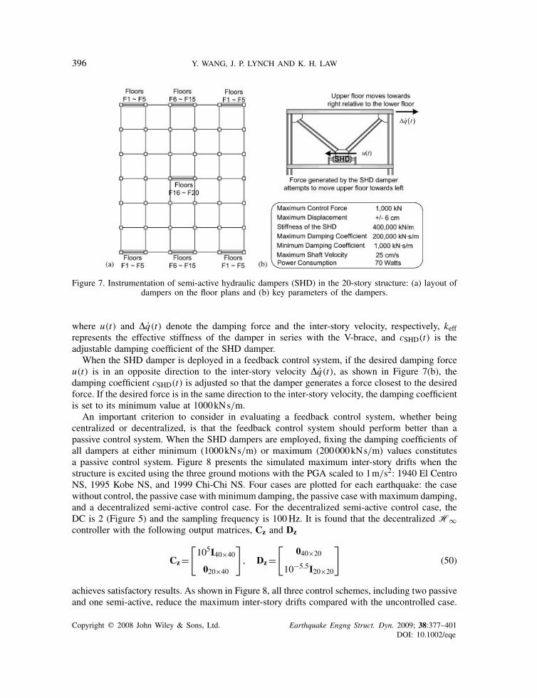
3.2.2. Simulation using SHD dampers. To investigate the performance of decentralized H∞control using realistic structural control devices, SHD dampers are employed in the simulations forthe 20-story structure. The arrangement of SHD dampers in the building is shown in Figure 7(a).From lower to higher floors, the number of instrumented SHD dampers decreases gradually from4 to 1. Figure 7(b) shows the installation of a SHD damper between two floors using a V-brace,together with key parameters of the damper. To accurately model the damping force, the Maxwellelement proposed by Hatada et al. [35] is employed. In a Maxwell element, a dashpot and astiffness spring are connected in series, which result in a damping force described by the followingdifferential equation:

u(t)+ keffcSHD(t)

u(t)=keff�q(t) (49)



Figure 7. Instrumentation of semi-active hydraulic dampers (SHD) in the 20-story structure: (a) layout ofdampers on the floor plans and (b) key parameters of the dampers.

where u(t) and �q(t) denote the damping force and the inter-story velocity, respectively, keffrepresents the effective stiffness of the damper in series with the V-brace, and cSHD(t) is theadjustable damping coefficient of the SHD damper.

When the SHD damper is deployed in a feedback control system, if the desired damping forceu(t) is in an opposite direction to the inter-story velocity �q(t), as shown in Figure 7(b), thedamping coefficient cSHD(t) is adjusted so that the damper generates a force closest to the desiredforce. If the desired force is in the same direction to the inter-story velocity, the damping coefficientis set to its minimum value at 1000kNs/m.

An important criterion to consider in evaluating a feedback control system, whether beingcentralized or decentralized, is that the feedback control system should perform better than apassive control system. When the SHD dampers are employed, fixing the damping coefficients ofall dampers at either minimum (1000kNs/m) or maximum (200000kNs/m) values constitutesa passive control system. Figure 8 presents the simulated maximum inter-story drifts when thestructure is excited using the three ground motions with the PGA scaled to 1m/s2: 1940 El CentroNS, 1995 Kobe NS, and 1999 Chi-Chi NS. Four cases are plotted for each earthquake: the casewithout control, the passive case with minimum damping, the passive case with maximum damping,and a decentralized semi-active control case. For the decentralized semi-active control case, theDC is 2 (Figure 5) and the sampling frequency is 100Hz. It is found that the decentralized H∞controller with the following output matrices, Cz and Dz

Cz=[105I40×40

020×40

], Dz=

[040×20

10−5.5I20×20

](50)

achieves satisfactory results. As shown in Figure 8, all three control schemes, including two passiveand one semi-active, reduce the maximum inter-story drifts compared with the uncontrolled case.



Figure 8. Maximum inter-story drifts for cases without control, with passive control (damping coefficientsof all SHD dampers fixed at minimum or maximum), and with decentralized semi-active control (DC=2

and 100Hz sampling frequency).

The passive control case with maximum damping generally results in less inter-story drifts thanthe passive case with minimum damping, except at a few higher floors for the El Centro and Kobeearthquakes. The decentralized semi-active control case not only effectively reduces drifts at lowerfloors, but also achieves greater mitigation of drifts at the higher floors compared with the twopassive cases. Better performance of the decentralized semi-active control case is observed for allthree earthquake records. For the Kobe earthquake, decentralized semi-active control reduces thedrift at the 18th story by about 75% compared with the uncontrolled and the two passive controlcases. This shows that in the passive case with maximum damping, dampers at each story mayonly attempt to reduce local responses and results in conflict among damper efforts at differentstories. While in the semi-active control case that aims to minimize the overall H∞-norm of theglobal structural system, efforts from dampers at different stories can be better coordinated toreduce overall structural response.

Figure 9 compares the performance indices for the 20-story structure instrumented with SHDdampers, when different control schemes are adopted. The two passive control schemes includethe maximum and minimum damping cases. To illustrate the effect of faster sampling frequency(i.e. shorter sampling periods) in decentralized feedback control, feedback control cases withdifferent centralization degrees (DC=1, . . . ,4) are associated with different sampling frequencies.For each centralization degree, the sampling frequency is selected in reverse proportion to thenumber of stories contained in one communication subnet (shown in Figure 5). For example, asampling frequency of 100Hz is associated with case DC2, while a sampling frequency of 50Hzis associated with the centralized case DC4 due to larger communication and computation burdens.



Figure 9. Simulation results for the 20-story SAC building instrumented with semi-active hydraulicdampers (SHD). The plots illustrate performance indices for passive control cases and semi-activefeedback control cases with different degrees-of-centralization (DC) and sampling frequencies:

(a) performance index J1 and (b) performance index J2.

The same three ground motion records scaled to a peak acceleration of 1m/s2 are used in thesimulation: 1940 El Centro NS, 1995 Kobe NS (JMA Station), and 1999 Chi-Chi. As shown inFigure 9, the feedback control cases generally achieve better performance when compared with thetwo passive control cases. Furthermore, the figure illustrates that although decentralized feedbackcontrol cases do not have complete sensor data available when calculating control decisions, theymay outperform the centralized case due to the faster sampling frequencies that are availablethrough decentralization. For example, compared with the centralized scheme DC4 (at 50Hz), thepartially decentralized scheme DC2 (at 100Hz) can provide larger reduction to both maximuminter-story drift and the 2-norm of the output vector zd.

4. SUMMARY AND CONCLUSION

This paper presents pilot studies in exploring decentralized structural control design that minimizesthe closed-loop H∞-norm. The decentralized control design offers promising solutions to large-scale structural sensing and control systems. Solutions are developed for both continuous-timeand discrete-time formulations. The properties of linear matrix inequalities are utilized to convertthe complicated decentralized H∞ control problem into a simple convex optimization problem.For such a convex optimization problem, decentralized architectures can be easily incorporatedto yield decentralized H∞ control solutions. Such solutions are necessary to provide controlsystems with the ability to scale with the number of sensors and actuators implemented in thesystem. Nevertheless, it should be noted that the shape constraining approach for decentralized



H∞ controller design is heuristic. The approach may not guarantee the minimum H∞-norm overthe complete solution space.

Numerical simulation results using a 3-story and a 20-story structure illustrate the feasibilityof the different decentralized control architectures. Comparison between the performance of thedecentralized H∞ controllers and the performance of decentralized LQR-based controllers illus-trates that both controllers deliver expected performance. Using the simulation results for the3-story structure, the trade-off between structural response attenuation and control effort is demon-strated for both the H∞ controllers and LQR controllers. The ratio of the required total actuatorcapacity over the building weight appears realistic for both types of controllers. For the 20-storystructure, the simulation results demonstrate that when realistic semi-active control devices (suchas the SHD dampers) are used in combination with the decentralized H∞ control algorithm, betterperformance can be gained over the passive control cases. It is also illustrated that decentralizedcontrol strategies may provide equivalent or even superior control performance, given that theircentralized counterparts could suffer longer sampling periods due to communication and computa-tion constraints. On the other hand, since the proposed control design is based on the assumptionof system linearity, further investigation on how to improve the control performance with nonlinearsemi-active control devices is needed.

The drawbacks of the presented decentralized H∞ control design include the inability toconsider the effect of time delay in the feedback loop and the requirement for inter-story drift andvelocity data for feedback. Future research in decentralized H∞ control may consider time delayeffects in the control algorithm and utilize system output feedback. Furthermore, dynamic outputfeedback will be explored instead of static feedback, to capitalize on a much larger controllerparametric space. Comparative studies will then be conducted between the decentralized H∞ anddecentralized LQR control designs with consideration of time-delay effects [12]. Future investiga-tion may also include developing a systematic method for the design of decentralized architectures,e.g. the delineation of overlapping subnets, as well as the selection of appropriate degrees ofcentralization.

ACKNOWLEDGEMENTS

This research is partially funded by the Office of Naval Research through the Young Investigator Awardreceived by Prof. Jerome P. Lynch at the University of Michigan. Part of the research was accomplishedduring Prof. Yang Wang’s PhD study at Stanford University, where he was supported by the Office ofTechnology Licensing Stanford Graduate Fellowship. This research is also partially supported by NSF,Grant Number CMMI-0824977 to Stanford University. The authors would like to thank Prof. Chin-HsiungLoh of the National Taiwan University for sharing the 3-story structure model, which is based on anexperimental structure built at the National Center for Research on Earthquake Engineering in Taiwan.Last but not least, the authors would like to thank the anonymous reviewers for their valuable commentsand suggestions.

REFERENCES

1. Soong TT. Active Structural Control: Theory and Practice. Wiley: Harlow, Essex, England, 1990.2. Spencer Jr BF, Nagarajaiah S. State of the art of structural control. Journal of Structural Engineering 2003;

129(7):845–856.3. Yao JTP. Concept of structural control. Journal of Structural Division (ASCE) 1972; 98(7):1567–1574.



4. Housner GW, Bergman LA, Caughey TK, Chassiakos AG, Claus RO, Masri SF, Skelton RE, Soong TT,Spencer Jr BF, Yao JTP. Structural control: past, present, and future. Journal of Engineering Mechanics 1997;123(9):897–971.

5. Chu SY, Soong TT, Reinhorn AM. Active, Hybrid, Semi-active Structural Control: A Design, ImplementationHandbook. Wiley: Hoboken, NJ, 2005.

6. Soong TT, Spencer Jr BF. Supplemental energy dissipation: state-of-the-art and state-of-the-practice. EngineeringStructures 2002; 24(3):243–259.

7. Sandell Jr N, Varaiya P, Athans M, Safonov M. Survey of decentralized control methods for large scale systems.IEEE Transactions on Automatic Control 1978; 23(2):108–128.

8. Siljak DD. Decentralized Control of Complex Systems. Academic Press: Boston, 1991.9. Lunze J. Feedback Control of Large Scale Systems. Prentice-Hall: Englewood Cliffs, NJ, 1992.

10. Shimizu K, Yamada T, Tagami J, Kurino H. Vibration tests of actual buildings with semi-active switching oildamper. Proceedings of the 13th World Conference on Earthquake Engineering, Vancouver, BC, Canada, 1–6August, 2004.

11. Kurino H, Tagami J, Shimizu K, Kobori T. Switching oil damper with built-in controller for structural control.Journal of Structural Engineering 2003; 129(7):895–904.

12. Wang Y, Swartz RA, Lynch JP, Law KH, Lu K-C, Loh C-H. Decentralized civil structural control using real-timewireless sensing and embedded computing. Smart Structures and Systems 2007; 3(3):321–340.

13. Wang Y. Wireless sensing and decentralized control for civil structures: theory and implementation. Ph.D. Thesis,Department of Civil and Environmental Engineering, Stanford University, Stanford, CA, 2007.

14. Skogestad S, Postlethwaite I. Multivariable Feedback Control: Analysis and Design. Wiley: Chichester, WestSussex, England, 2005.

15. Balandin DV, Kogan MM. LMI-based optimal attenuation of multi-storey building oscillations under seismicexcitations. Structural Control and Health Monitoring 2005; 12(2):213–224.

16. Chase JG, Smith HA. Robust H∞ control considering actuator saturation. I: theory. Journal of EngineeringMechanics 1996; 122(10):976–983.

17. Jabbari F, Schmitendorf WE, Yang JN. H∞ control for seismic-excited buildings with acceleration feedback.Journal of Engineering Mechanics 1995; 121(9):994–1002.

18. Lin C-C, Chang C-C, Chen H-L. Optimal H∞ output feedback control systems with time delay. Journal ofEngineering Mechanics 2006; 132(10):1096–1105.

19. Mahmoud MS, Terro MJ, Abdel-Rohman M. An LMI approach to H∞-control of time-delay systems for thebenchmark problem. Earthquake Engineering and Structural Dynamics 1998; 27(9):957–976.

20. Johnson EA, Voulgaris PG, Bergman LA. Multiobjective optimal structural control of the Notre Dame buildingmodel benchmark. Earthquake Engineering and Structural Dynamics 1998; 27(11):1165–1187.

21. Narasimhan S, Nagarajaiah S. Smart base isolated buildings with variable friction systems: H∞ controller andSAIVF device. Earthquake Engineering and Structural Dynamics 2006; 35(8):921–942.

22. Yang JN, Lin S, Jabbari F. H∞-based control strategies for civil engineering structures. Structural Control andHealth Monitoring 2004; 11(3):223–237.

23. Wang S-G. Robust active control for uncertain structural systems with acceleration sensors. Journal of StructuralControl 2003; 10(1):59–76.

24. Chase JG, Smith HA, Suzuki T. Robust H∞ control considering actuator saturation. II: applications. Journal ofEngineering Mechanics 1996; 122(10):984–993.

25. Boyd S, El Ghaoui L, Feron E, Balakrishnan V. Linear Matrix Inequalities in System and Control Theory. SIAM:Philadelphia, PA, 1994.

26. Zhou K, Doyle JC, Glover K. Robust and Optimal Control. Prentice-Hall: Englewood Cliffs, NJ, 1996.27. Gahinet P. LMI Control Toolbox for Use with MATLAB. MathWorks Inc.: Natick, MA, 1995.28. Grant M, Boyd S. CVX: Matlab software for disciplined convex programming (web page and software).

http://stanford.edu/∼boyd/cvx (18 June 2008).29. Franklin GF, Powell JD, Workman ML. Digital Control of Dynamic Systems. Addison-Wesley: Menlo Park, CA,

1998.30. Kim J-H, Jabbari F. Actuator saturation and control design for buildings under seismic excitation. Journal of

Engineering Mechanics 2002; 128(4):403–412.31. Barroso LR, Chase JG, Hunt S. Resettable smart dampers for multi-level seismic hazard mitigation of steel

moment frames. Journal of Structural Control 2003; 10(1):41–58.32. Kannan S, Uras HM, Aktan HM. Active control of building seismic response by energy dissipation. Earthquake

Engineering and Structural Dynamics 1995; 24(5):747–759.



33. Burl JB. Linear Optimal Control: H2 and H∞ Methods. Addison-Wesley Longman: Menlo Park, CA, 1999.34. Spencer Jr BF, Christenson RE, Dyke SJ. Next generation benchmark control problem for seismically excited

buildings. Proceedings of the 2nd World Conference on Structural Control, Kyoto, Japan, 29 June–2 July 1998.35. Hatada T, Kobori T, Ishida M, Niwa N. Dynamic analysis of structures with Maxwell model. Earthquake

Engineering and Structural Dynamics 2000; 29(2):159–176.


Decentralized H controllerdesignforlarge …jerlynch/papers/HinfEESD.pdf · 378 Y. WANG, J. P....

Documents

Transcript of Decentralized H controllerdesignforlarge …jerlynch/papers/HinfEESD.pdf · 378 Y. WANG, J. P....