Decentralization and the Gamble for Unity - … · Decentralization and the Gamble for Unity...
56
Decentralization and the Gamble for Unity Michael Gibilisco * September 15, 2017 Abstract I reconcile competing accounts of decentralization and its effect on secession- ist mobilization by endogenizing the regional minority’s grievance level in a dynamic framework. I demonstrate that decentralized institutions may have higher rates of minority unrest than their more centralized counterparts, and vice versa. Federations with moderate levels of power-sharing arrangements are particularly prone to secessionist violence. Even optimally chosen levels of decentralization can be followed by outbursts of minority protest or rebel- lion as the government subsequently refrains from repression in order to gen- erate enough good will for a lasting peace. More broadly, grievances have a non-monotonic relationship with the onset and duration of secessionist con- flict, which is one explanation for their elusive relationship in the greed versus grievance debate. * University of Rochester Department of Political Science. Harkness Hall 333, Rochester NY 14627. Email: [email protected]
Transcript of Decentralization and the Gamble for Unity - … · Decentralization and the Gamble for Unity...
Decentralization and the Gamble for Unity
Michael Gibilisco∗
September 15, 2017
Abstract
I reconcile competing accounts of decentralization and its effect on secession-ist mobilization by endogenizing the regional minority’s grievance level in adynamic framework. I demonstrate that decentralized institutions may havehigher rates of minority unrest than their more centralized counterparts, andvice versa. Federations with moderate levels of power-sharing arrangementsare particularly prone to secessionist violence. Even optimally chosen levelsof decentralization can be followed by outbursts of minority protest or rebel-lion as the government subsequently refrains from repression in order to gen-erate enough good will for a lasting peace. More broadly, grievances have anon-monotonic relationship with the onset and duration of secessionist con-flict, which is one explanation for their elusive relationship in the greed versusgrievance debate.
∗University of Rochester Department of Political Science. Harkness Hall 333, Rochester NY14627. Email: [email protected]

1 Introduction
Decentralization, or a similar type of home-rule institution, offers one of the most
promising solutions to conflict in ethnically divided societies. Federalist institutions
preserve the integrity of the state, avoiding the costly alternatives of repression or
civil violence. Diverse regimes such as Spain, India, and China devolve authority to
more localized units, and both the number of decentralized territories and the scope
of their delegated powers are on the rise (Arzaghi and Henderson 2005; Rodden
2004).
Despite its importance, there is little scholarly consensus on the effectiveness of
decentralization in multiethnic states. While some theories paint it as a long-term,
stabilizing solution to conflict (Hechter 2000; Lijphart 1977; Lustick, Miodownik
and Eidelson 2004), others consider it a potentially violent interlude along the path
to secession (Bunce and Watts 2005; Cornell 2002; Kymlicka 1998; Roeder 2009).
Consistent with both claims, researchers find that decentralization has mixed and,
at times, contradictory effects on a variety phenomena related to secessionist mobi-
lization including protests (e.g., Saideman et al. 2002), rebellions (e.g., Cederman
et al. 2015; Siroky and Cuffe 2014), ethnoterritorial parties (e.g., Brancati 2006;
Meguid 2015), and regional identities (e.g., Cole 2006; Elkins and Sides 2007).
In this paper, I show that these apparently contradictory accounts are, in fact,
consistent with each other. I construct a dynamic game in which per-period inter-
action is explicitly shaped by endogenous levels of grievance, that is, the minority’s
latent animosity toward the central government. In particular, I incorporate two fea-
tures of intergroup resentment that appear essential for a theory of conflict. First,
grievances arise through the emotional legacy of conflict, rivalry, and disenfranchise-
ment (Hale 2008; Horowitz 1985; Petersen 2002; Wimmer, Cederman and Min 2009).
Thus, hostile policies associated with preventive repression, such as the suspension
of civil liberties, fuel psychological tensions between the majority and minority. In
contrast, more accommodative policies, such as decentralization, allow the tensions
to soften over time. Second, grievances are politically exploitable. A regional elite
may use its group’s antipathy toward the central government to overcome collective
action problems and mobilize a populace for secession (Cederman, Weidmann and
Gleditsch 2011; Hechter, Pfaff and Underwood 2016).1
Although I am not the first to study the relationships among ethnic conflict,
decentralization, and historical grievances, I endogenize all three in an explicitly dy-
namic framework, demonstrating how the key features of group antipathy determine
1Several authors document such an effect in countries with secessionist groups (Araj 2008;Benmelech, Berrebi and Klor 2015; Bloom 2004; Dugan and Chenoweth 2012; Gil-Alana and Barros2010; LaFree, Dugan and Korte 2009; Zussman and Zussman 2006). More broadly, Opp (1988),and Opp and Roehl (1990) detail survey evidence linking grievances to the support of protestersand their policy goals. Blattman (2009) and Lyall, Blair and Imai (2013) demonstrate that stateviolence increases political participation and decreases support for the regime.
1

the government’s long-term treatment of minorities. Government policies and their
effects on minority grievances reinforce each other over time. On the one hand, re-
pressive policies increase the minority’s resentment toward the central government,
and hence its mobilization capacity, magnifying the future security benefits of repres-
sion. On the other hand, by abstaining from repression and tolerating protests, the
government may reduce minority resentment toward peaceful levels, attenuating the
future security costs associated with permitting said protests. Thus, governments
face a dynamic trade-off between long-term peace and short-term security. While
repression deters the threat of secession today, it increases grievances tomorrow,
moving majority-minority relations further away from peace. If minority grievances
are not too large, then the incentive for peace dominates the incentive for security,
and the government gambles for unity. That is, it tolerates secessionist mobilization
in the short run in order to establish enough amity for a stable peace in the long
run.
Whether or not the government’s optimal strategy involves gambling for unity
depends critically on the degree of decentralization. By credibly allocating regional
control away from the central government to the minority, federalist institutions
reduce the stakes of center-periphery conflicts. This makes gambling for unity more
appealing through two channels. The first is obvious; as the government’s relative
benefit from controlling the region’s resources or policies decreases, it tolerates a
higher risk of secession, avoiding costly repression. The second is more nuanced.
Decreasing the minority’s relative benefit from independence dissuades the group
from mobilizing at smaller grievance levels, where its capacity for mobilization is
depleted. Because of this, decentralization increases the speed at which grievances
dissipate to peaceful levels, thereby diminishing the security costs associated with
the gambling for unity strategy. Thus, the government grants some degree of regional
autonomy if it plans to reduce grievances in the subsequent interaction.
The baseline model I construct captures these interactions by treating minor-
ity grievances like a capital stock, fueled by preventative repression but potentially
weakened in repression’s absence. While anticipating the endogenous evolution of
intergroup animosity, a central government and a peripheral minority struggle to
control a regional territory in each of an infinite number of periods. Within each
period, the government chooses whether to preemptively repress the minority, grant
it independence or take a hands-off approach. Subsequently, if preventative repres-
sion is not used, then the group determines whether or not to engage in secessionist
mobilization, and the probability that such efforts succeed increases with the group’s
grievance. I then allow the government to create constitutionally guaranteed power-
sharing institutions, where it may credibly commit to some level of decentralization
at the beginning of the interaction.
2

I characterize two results that resolve the contradictory accounts of decentral-
ization and its effectiveness. First, exogenous one-off shifts in decentralization levels
have non-monotonic effects on the incidence of secession. In other words, decentral-
ized institutions may have higher rates of minority unrest than their more centralized
counterparts, and vice versa. In particular, states with moderate levels of decentral-
ization are more susceptible to secessionist violence than those with small or large
levels. Second, I consider the government’s optimal decentralization level and its
associated risk of secession in the subsequent interaction. I show that there exist
equilibria in which the government grants some degree of regional autonomy and
deters the threat of secession, as in the United Kingdom after devolution in the late
1990s. In other equilibria, however, positive levels of decentralization, even when
optimally chosen by the central government, do not deter the threat of secession and
may encourage minority mobilization, as in the Basque Country after the adoption
of the Spanish Constitution. Thus, outbursts of minority unrest after exogenous and
endogenous decentralization are entirely consistent with both theoretical accounts.
The theory not only reconciles competing visions of federalism, but it also endo-
genizes several variables of interest including grievances, minority-initiated conflict
and government repression, generating several substantive implications. In equi-
librium, grievances have a non-monotonic effect on the incidence of secessionist
conflict, where only moderately aggrieved minorities mobilize, thus providing a the-
ory for their heretofore elusive empirical relationship (Blattman and Miguel 2010;
Fearon and Laitin 2003; Laitin 2007). With small grievances, the result is obvious
as mobilization offers the group little to no benefits. With moderate grievances, the
government gambles for unity, so minority unrest erupts. In contrast, with large
grievances, the security costs associated with gambling for unity are substantial,
so the government preempts unrest by using repression or granting independence.
Likewise, I demonstrate that governments devolve power only to moderately ag-
grieved groups, a result similar to the relationship between democratization and
inequality in Acemoglu and Robinson (2005). Furthermore, when the government
does optimally decentralize, moderate increases in minority animosity lead to gov-
ernment to respond by devolving greater levels of decentralized powers, a pattern
consistent with asymmetric federalism in Spain and India. Finally, I show that the
government and minority group can enter cycles of repression and mobilization. In
these cycles, grievances have a non-monotonic effect on repression, where the gov-
ernment represses at a small grievance level but tolerates mobilization are a larger
level. While these cycles are often attributed to tit-for-tat behavior (e.g., Haushofer,
Biletzki and Kanwisher 2010), they emerge in this simpler setting, which excludes
these types of punishment strategies.
Furthermore, my theory builds upon previous work analyzing intergroup an-
imosity and center-periphery relationships in three directions (Cederman, Weid-
3
mann and Gleditsch 2011; Hale 2008; Hechter, Pfaff and Underwood 2016; Horowitz
1985; Petersen 2002; Wimmer, Cederman and Min 2009). First, I analyze both the
strategic and emotional aspects of center-periphery relations in a unified framework
rather than separating the two considerations.2 As mentioned above, this gener-
ates new hypotheses concerning the key variables of interest. Second, other game
theoretic approaches to ethnic violence rely on explanations that apply to conflicts
or bargaining failures more generally, e.g., incomplete information or commitment
problems (Fearon 2006; Walter 2009a). As I demonstrate below, secessionist wars
can erupt in this model’s equilibrium even when the government credibly commits
to future power-sharing institutions and has complete information about the minor-
ity’s preferences. Thus, by focusing on group hatred, the theory highlights a causal
factor that is potentially more unique to ethnic disputes than to interstate or other
forms of conflict, where group emotions arguably play less of a role. Third and
highly related, previous theories of secession traditionally emphasize the stakes of
regional control (Collier and Hoeffler 2006; Muller and Seligson 1987; Walter 2009b;
Wimmer 2002) and whether or not minority mobilization is feasible or cost-effective
(Fearon and Laitin 2003; Tarrow 1994). While these are both important parameters
in the model, I add to this body of work by characterizing the effects of regional
grievances on the long-term evolution civil conflict and the government’s optimal
policy response.
This paper proceeds as follows. I close this section by briefly differentiating
my approach from previous models of grievance, repression, and decentralization.
In Section 2, I construct a dynamic theory of grievances, and Section 3 contains
the main results of the baseline model. In Section 4, I study the effects of de-
centralization on minority unrest and analyze the government’s optimal level of
decentralization. Section 5 concludes.
1.1 Models of Grievance and Decentralization
Attempting to capture the emotional concerns described above, scholars endoge-
nize group hatred and conflict in a political economy framework, but they examine
finite-period interactions between groups. For example, Shadmehr (2014) inves-
tigates backlash protests after repression and finds a non-monotonic relationship
between economic inequality and repression. Similarly, although they do not focus
on group psychologies, several authors model counterproductive repression (Bueno
De Mesquita 2005b; Bueno de Mesquita and Dickson 2007; Dragu and Polborn 2014;
2For example, when criticizing rational choice approaches, Horowitz writes “economic theoriescannot explain the extent of the emotion invested in ethnic conflict” (1985, p. 134) and “a bloodyphenomenon cannot be explained by a bloodless theory” (1985, p. 140). In addition, Hale concludesthat “explanations of ethnic politics, then, must divorce ethnicity from the realm of motives (desires,preferences, values) at the same time that they introduce into the realm of strategy....” (2008, p.3).
4

Lichbach 1987). In addition, Amegashie and Runkel (2012) develop a two-period
contest model, where the fighting in the first period generates “revenge” rewards
in the second, and Glaeser (2005) considers the signaling incentives of hate speech
in campaigns. Unlike these theories, I endogenize the tensions between majority
and minority groups in a fully dynamic model. In this environment, the majority’s
benefit from tolerating minority mobilization arises from the future prospects of a
long-term peace. In contrast, finite environments do not account for these benefits
when the majority may not expect grievances to sufficiently dissipate after a single
interaction.
When explaining decentralization, several theories abstract away from group
conflict by analyzing the trade-offs between large countries with economies of scale
or a central planner and smaller ones with better targeted local policies (e.g., Alesina
and Spolaore 1997; Bolton and Roland 1997; Oates 1972). Several scholars expand
these models to include bargaining on the federal level (Besley and Coate 2003;
Lockwood 2002) or legislative voting on federal directives (Loeper 2013). Similarly,
Bednar (2007) studies the efficiency of federalism in a repeated public goods set-
ting, and others describe how decentralization can reduce corruption (e.g., Edwards
and Keen 1996) or prevent governments from interfering with markets (e.g., Qian
and Weingast 1997). Anesi and De Donder (2013) consider secessionist wars and
accommodative policies, but in their framework, the minority group never mobilizes
after majorities adopt accommodative policies in equilibrium. Bueno De Mesquita
(2005a) also models why governments concede to regional groups even though the
concessions subsequently increase the intensity of center-periphery conflict. His
approach requires more complicated history-dependent strategies in which govern-
ments cannot commit to concessions without a future threat of minority violence.
In contrast, my analysis does not rely on an equilibrium construction with folk-
theorem-like properties, and I model decentralization as a credible commitment,
reflecting the situations in countries such as Spain and India with constitutionally
guaranteed power-sharing institutions.
Finally, this paper is also related to other dynamic models of contentious politics.
Harish and Little (2017) consider a model of opposition violence in elections where
two parties interact over an arbitrarily large number of periods, rotating in and out
of office. Using infinitely repeated environments, Acemoglu and Robinson (2005)
investigate regime transitions, and Fearon (2004) uses a similar approach to analyze
civil wars.3 In these two papers, the degree to which actors successfully mobilize or
win wars is drawn i.i.d. across periods. In contrast, the theory constructed below
incorporates a fully endogenous state variable, i.e., grievances, that determines the
degree to which minority unrest results in successful secession. This introduces a
3In static environments, Boix (2003) and Shadmehr (2014) adopt similar modeling strategies.The latter separates the Periphery’s mobilization and revolution decisions, and the former modelsthe effectiveness of repression as private information, introducing signaling incentives.
5

rich dynamic trade-off between short-term security and a long-term peace for the
central government. In addition, the model exhibits considerable path dependence,
where a single equilibrium exhibits several patterns of center-periphery relationships
depending on the initial level of grievances.
2 A Theory of Minority Grievances
A central government, which I call the Center and label C, and a peripheral elite,
which I call the Periphery and label P , struggle to control a regional territory or
policy.4 The two groups interact for an infinite number of periods t = 1, 2, . . . They
discount future interactions by δ ∈ (0, 1).
Period t’s interaction is characterized by a commonly observed, two-dimensional
state variable xt = (st, gt). The first dimension is a binary variable st ∈ {P,C},denoting the actor who controls the territory initially in the period. The second
dimension, gt ∈ N0, describes the regional population’s current level of grievance—
or animosity toward the central government. I use grievance, animosity, spite, etc.
interchangeably hereafter. Grievances determine the probability with which seces-
sionist mobilization succeeds if launched by the Periphery. Label this probability
F (gt), where F is strictly increasing in gt. In other words, grievances determine the
Periphery’s capacity for mobilization, and a secessionist movement more likely suc-
ceeds as the region become more aggrieved. While I focus on secession throughout,
mobilization can be interpreted more broadly as an attempt to force concessions from
the central government, and this can include protest, violence, war, or even support
for a separatist party. Furthermore, assume that secession is impossible when the
local population has no grievances, i.e., F (0) = 0, and that p ∈ (0, 1] describes the
maximum capabilities of a secessionist movement, i.e., limg→∞ F (g) = p.
Once the Periphery gains control over its territory or policy (st = P ), it retains
control in the subsequent interaction (st′
= P for all t′ > t). In other words,
independence is an absorbing state, essentially ending the game.5 In contrast, if
the Center controls the regional territory in period t, i.e., st = C, then Figure 1
describes the interaction within the period, which proceeds as follows.
1. The Center and the Periphery observe grievance gt ∈ N0.
2. The Center chooses policy rt ∈ {∅, 0, 1}, deciding whether to grant indepen-
dence (rt = ∅), use preemptive repression (rt = 1), or pursue a hands-off
approach (rt = 0).
4In Spain, the Center would be the Spanish government, and the Periphery could be secessionistleaders in either the Basque Country or Catalonia. In colonial India, the two actors are the Britishgovernment and Indian independence leaders, respectively. The Center could also be the Israeligovernment, and the Periphery a Palestinian liberation faction such as Fatah or Hamas.
5This assumption is standard in models of rebellion and civil war (e.g., Acemoglu and Robinson2005; Fearon 2004; Shadmehr 2014, 2015) and adds tractability to the subsequent analysis.
6

Figure 1: A period of interaction under the Center’s control.
gt C P
(0,
πPP1−δ
)
(πCC − κC , πCP
)gt+1 = gt + 1
(πCC , π
CP
)gt+1 = max{gt − 1, 0}
(πCC , π
CP − κP
)
(−ψ, π
PP
1−δ − κP)
gt+1 = max{gt − 1, 0}
Period t+ 1Period t
rt = 0
rt = ∅
rt = 1
mt = 0
mt = 1
1-F (gt)
F (gt)
Caption: For the Center, rt = ∅ denotes grant independence, rt = 1 repression, and rt = 0 takea hands-off approach. For the Periphery, mt = 1 denotes mobilize and mt = 0 no mobilization.Circles refer to histories after which the Periphery gains independence, i.e., st
′= P , for all periods
t′ > t.
3(a) If the Center grants independence (rt = ∅), then the interaction ends with
the Periphery gaining control over the region in the next period (st+1 = P ).6
3(b) If the Center represses (rt = 1), then Center retains control of the territory
(st+1 = C).7
3(c) If the Center neither represses nor grants independence (rt = 0), then the Pe-
riphery takes action mt ∈ {0, 1} and decides to mobilize a secessionist move-
ment (mt = 1) or not (mt = 0). With probability F (gt), mobilization suc-
ceeds, and the Periphery gains independence (st+1 = P ). With complimentary
probability, mobilization fails, and the territory remains under Center control
(st+1 = C).
Payoffs are as follows. First, repression and mobilization are costly, and they
entail per-period costs κC and κP for the Center and Periphery, respectively. In
addition, actor i receives per-period benefit πji ≥ 0 when j controls the territory,
6Below, I make independence a continuous variable capturing the degree of autonomy or de-centralization.
7In this framework, repression is “controlling or eliminating specific challenges (real or imag-ined) to existing political leaders, institutions, and/or practices” (Davenport 2007, p. 3). Such anassumption captures asymmetric power relations where repression temporarily removes the Periph-ery’s ability to coordinate for collective action. This is similar to other models of repression (e.g.,Acemoglu and Robinson 2005; Boix 2003; Shadmehr 2014). See Davenport (2007) and Earl (2011)for other definitions of repression.
7

and I normalize the Center’s benefit under Periphery-control to zero, πPC = 0.8
The benefits can include the region’s tax surplus or control over its linguistic or
cultural policies, which carry their own similarly tangible benefits such as trade,
employment opportunities, etc. Because independence is an absorbing state, if the
Periphery gains control over the region, then actors receive total future benefits
πPi + δπPi + δ2πPi + . . ., which reduces toπPi1−δ . Accordingly, Figure 1 reports these
total benefits after histories in which the Periphery gains territorial control, i.e.,
those with Center-granted independence or successful mobilization. Finally, if the
Periphery successfully mobilizes a secessionist movement, then the Center receives
a cost −ψ, where the parameter ψ > 0 captures the Center’s preference for Center-
initiated independence over an often times messier secessionist movement.9
As long as the Center retains its control over the local territory, the interac-
tion within each period remains the same. Nonetheless, grievances change endoge-
nously and evolve according to the history of government repression. To capture
this, I assume that repression today increases the Periphery’s animosity toward the
Center tomorrow, but this animosity decreases in the absence of repression.10 For-
mally, if today’s grievances are gt and the Center chooses policy rt, then tomorrow’s
grievances, gt+1, take the form:
gt+1 =
gt + 1 if rt = 1
max{gt − 1, 0} otherwise.
This formalization has an intuitive interpretation.11 In the short run, preemptive
repression, such as the suspension of civil liberties or military occupation, prevents
regional protests and mobilization within period t, but in the long run, repression
increases regional grievances in period t+1. When the Center refrains from repress-
ing the regional populace, their resentment towards the government depreciates
although the Periphery may protest in the current period. Large grievance levels re-
sult in a Periphery with a stronger capacity for protests and mobilization, and small
levels diminish this capacity. Although it may appear that this construction as-
sumes repression has no persistent benefits, this is not the case. In fact, repression’s
benefits persist for an entire period. Because the length of a period is arbitrary, the
8It is also possible to normalize the Periphery’s payoff of Center control, i.e., πCP to zero as well.Avoiding this normalization makes the decentralization application in Section 4 more intuitive,however.
9The substantive results would not change if the Center received cost −ψ after any mobilizationregardless of its success.
10If grievances depreciate with probability β ∈ (0, 1] after the government refrains from repres-sion, then the substantive results of the model would not change.
11Adding one unit of grievance after repression may appear restrictive. Nonetheless, I placerelatively mild assumptions on the mapping from grievances to secessionist capabilities, i.e., F ,which can capture a host of interpretations such as increasing or decreasing returns to grievance.
8

model captures situations in which repression’s security benefits deteriorate more
quickly than its effects on regional grievances.
I characterize sub-game perfect equilibria in stationary Markovian strategies
(equilibria, hereafter), as is standard in these dynamic games.12 In this game,
such strategies describe behavior in which the Center controls the regional territory
(st = C), which means they can be written as functions of gt. Because they are
stationary, I drop references to time periods hereafter. Allowing for mixing, such
a strategy for the Center is a function σC : {∅, 0, 1} × N0 → [0, 1]. Here, σC(r; g)
denotes the probability that the Center chooses policy r ∈ {∅, 0, 1} at grievance g.
For the Periphery, a strategy is a function σP : N0 → [0, 1], where σP (g) denotes
the probability with which the Periphery mobilizes. A strategy profile σ is a pair
σ = (σC , σP ). Finally, V σi (g) denotes i’s continuation value from beginning the
game in state x = (C, g) with both actors subsequently playing according to profile
σ. Appendix A contains formal statements of expected utilities and the equilibrium
definition.
Throughout, I focus the analysis on interesting cases, barring certain parameter
values leading to trivial interaction. This focus translates into two assumptions.
First, the Periphery’s cost of mobilization cannot be arbitrarily large as to drown
out any value of regional control. Second, the Center’s cost of a successful seces-
sionist movement cannot be arbitrarily small, or else it has no incentive to prevent
mobilization. Assumptions 1 and 2 explicitly state these conditions.13
Assumption 1 The Periphery values independence, that is, πPP − πCP > (1−δ)κPp .
In words, the condition implies that the Periphery mobilizes with very large
grievances if the Center were to never grant independence. Obviously, this occurs
when the Periphery values self-determination, that is, πPP−πCP is large, and actors are
patient. The next assumption says that successful secessionist movements impose
non-trivial costs on the Center.
Assumption 2 Secession is costly, that is, ψ > min{πCC (1−p)
p ,(1−δ)κC−p(πCC−δκC)
p(1−δ)
}.
In words, the inequality implies that the Center prefers to use repression or grant
independence rather than risk secessionist mobilization at very large grievances.
Such an assumption is satisfied when p = 1, that is, the probability of a successful
movement goes to one as grievances become very large. With these preliminary
considerations clarified, I proceed to the analysis of the game in the next section.
Subsequently, I expand the model to include decentralization.
12Because the model is a dynamic game with finite actions and a countable state space, anequilibrium exists, albeit in mixed strategies (Federgruen 1978).
13Below, I also discuss how behavior changes without these assumptions.
9

3 Repression and the Evolution of Grievances
In this section, I characterize equilibria of the baseline model. I first construct a
necessary condition on the level of grievance for the Periphery to mobilize and the
government to repress or grant independence. To do this, consider the cutpoint g†
defined as
g† = max
{g ∈ N0 | κP ≥ F (g)
πPP − πCP1− δ
}.
Because F is strictly increasing, g† exists and is unique if and only if Assumption
1 holds. Throughout, I say grievance g is small (large) if g ≤ g† (g > g†). In
this baseline model, I focus on the generic case where κP > F(g†) πPP−πCP
1−δ , but this
assumption is appropriately relaxed in the extended version with decentralization.
Lemma 1 If grievances are small, then the Periphery never mobilizes, and theCenter neither represses nor grants independence. That is, g ≤ g† implies σP (g) = 0and σC(0; g) = 1 in every equilibrium σ.
The Appendix contains the Lemma’s proof and those of all subsequent results.
Intuitively, the Periphery mobilizes with probability zero at grievance g if mobiliza-
tion’s costs are larger than its benefits, that is,
κP > F (g)
[πPP
1− δ− πCP − δV σ
P (g − 1)
].
The right-hand-side of the inequality denotes the marginal benefits of mobilization
at grievance g, where the Periphery compares its value of winning independence to
its value of remaining in the country and weights this difference by the probability
of success. Because the Periphery can choose to never mobilize in all future periods,
in which case its stage payoff does not depend on σC , V σP (g − 1) is bounded below
byπCP1−δ in any equilibrium σ. Combining this lower bound with the inequality above
reveals that the Periphery will never mobilize with small grievances.
Whether large grievances are sufficient for mobilization depends on the Center’s
strategy. For example, if the Periphery expects the Center to grant independence
or to repress and substantially inflate its grievances, then the Periphery may refrain
from mobilizing today because it expects either independence or a greater mobi-
lization capacity in future periods, respectively. Which of these possibilities can be
realized in equilibrium depends the Center’s cost of repression. The cost of repres-
sion varies across countries depending on a host of factors including the Periphery’s
distance from the Center, the Center’s bureaucratic and military capabilities, and
the type of terrain within the region (Fearon and Laitin 2003).
To distinguish two cases, say the regime is strong if the cost of repression is small,
10

that is, κC < πCC . Likewise, the regime is weak if the cost of repression is large, that
is, κC > πCC . In other words, a regime is strong when the central government can
effectively repress the minority group and still retain a profit from regional control.
In contrast, weak regimes have low military capabilities or a considerable distance
to the region, and repressing the minority group entails prohibitive costs.
Strong and weak regimes exhibit considerably different dynamics. Because of
this, I characterize equilibria in each regime separately. In strong regimes, the results
below demonstrate that equilibrium behavior is not only in pure strategies but also
unique. In weak regimes with intense grievances, in contrast, equilibrium behavior
may not be unique and may involve mixing, though all equilibria produce identical
behavior at more moderate grievance levels.
3.1 Strong Regimes
In strong regimes, the Center never grants independence, as it can always repress
the Periphery and receive some positive concessions from keeping the country to-
gether. Although the Center always has repression as a beneficial recourse, it may
refrain from using it and instead reduce grievances to levels that ensure a peaceful
interaction. When this happens, the Center may risk secession in the short run in
order to obtain a lasting peace in the long run. More formally, the Center deter-
mines at what grievance g does the payoff from repression outweigh the payoff from
letting minority spite dissipate to peaceful levels below g†. Because the Periphery’s
capacity for mobilization increases with its animosity toward the government, the
Center’s equilibrium strategy exhibits a strong monotonicity property as the next
proposition demonstrates.
Proposition 1 In strong regimes, there exists cutpoint g∗ ∈ R such that g∗ > g†
and the following hold in every equilibrium σ.
1. The Periphery mobilizes if and only if grievances are large, i.e., if g > g†, thenσP (g) = 1 and if g ≤ g†, then σP (g) = 0.
2. If g < g∗, then the Center neither represses nor grants independence, i.e.,σC(0; g) = 1, and grievances depreciate toward zero.
3. If g > g∗, then the Center uses repression, i.e., σC(1; g) = 1, perpetuatinggrievances toward positive infinity.
4. Secession occurs with positive probability along the path of play if and only ifgrievance are moderate, i.e., g† < g < g∗.
Thus, the equilibrium’s dynamics reveal considerable path dependence in the
sense that observable behavior and the evolution of grievances change considerably
as initial grievances, g1, vary. This is illustrated in Figure 2, which graphs the
equilibrium path of play as a function of intergroup tensions. In the figure, the
11

Figure 2: The equilibrium path of play in strong regimes (Proposition 1).
g∗g+1 g + 1 g + 2g − 1g†g − 3
1 -F (g)
F (g)
secession
1 -F (g - 1)
F (g - 1)
secession
horizontal line represents the possible grievance levels, and the arrows describe how
the game transitions between grievances and whether the region gains independence.
When g1 is small, no protests occur by Lemma 1. This alleviates the need for
repression, grievances depreciate in all future periods, and the country remains
unified over time. When g1 is moderately large (g† < g1 < g∗), the Center does
not repress, because it gambles for the country to enter the peaceful states below
g† without breaking apart. In this case, regional protests erupt, and the country
remains unified with probability strictly less than one. Finally, when g1 is more
intense (g1 > g∗), the country is unlikely to enter the unified peaceful states, so
the Center uses repression to prevent mobilization. In this last case, intergroup
hostilities increase, but the country remains unified through long-term repression.
Thus, the evolution of grievance is particularly stark in strong regimes. This
may raise questions concerning the degree to which the result is robust to changes
in the underlying modeling choices. To gain some leverage on an answer, I show
that the equilibrium in Proposition 1 is strict, that is, in the equilibrium, each actor
has a unique best-reply at every grievance level.14 As such, continuous changes in
the model’s payoffs and transition probabilities will have no effect on equilibrium
strategies as long as the perturbations are sufficiently small. This covers a series
of robustness checks. For example, the model could incorporate a random, discrete
shock to the grievance variable in each period. Likewise, backlash mobilization may
erupt after repression with a certain probability, which is similar to ensuring that
the Center’s payoff from repression decreases with larger grievances. When these
shocks are sufficiently small, Proposition 1 describes equilibrium strategies in the
extended model, although the path of play becomes more complicated due to the
additional stochastic processes.
Furthermore, the proposition requires both the costly secession and valuable
independence assumptions. If they do not hold, then the equilibrium is strategically
trivial. If Assumption 1 fails, then all grievances are small, and Lemma 1 describes
equilibrium strategies. On the other hand, if Assumption 2 fails, then the Periphery
14The Supplementary Information contains a formal definition and proof; it can be found atmichaelgibilisco.com/research
12

mobilizes if and only if grievances are large, but the Center never represses because
it has no incentive to prevent mobilization.
Proposition 1 has two implications concerning how grievances relate to repres-
sion and secession. First, there is a non-monotonic relationship between grievances
and the probability of secessionist mobilization, providing one reason for their elu-
sive empirical relationship (Blattman and Miguel 2010; Collier and Hoeffler 2004;
Dixon 2009; Fearon and Laitin 2003). A selection effect emerges, because the Center
preempts mobilization with intense grievances, generating the monotonicity. Hence,
regional activists who attempt to provoke repression (e.g., Bueno de Mesquita and
Dickson 2007; Kydd and Walter 2006) have a complicated decision. Specifically,
there is a “window of opportunity” for regional grievances to be effective and se-
cession to occur with positive probability. Furthermore, these non-linearities have
initial empirical support. For example, Hegre and Sambanis (2006) find only mod-
erate values of grievance increase the likelihood of civil war. In addition, Lacina
(2014) investigates violence in India during federalization and concludes that “a lin-
ear relationship between objective measures of grievance and militancy is therefore
thwarted by governments’ credible threat of repression against the most marginal,
aggrieved interests” (p. 733).
Second, the proposition suggests that time-series data of repression and mobi-
lization may inspire greater confidence in repression’s long-term effectiveness (e.g.
Benmelech, Berrebi and Klor 2015; Dugan and Chenoweth 2012; Haushofer, Bilet-
zki and Kanwisher 2010; Lyall 2009). In equilibrium today’s repression implies
decreased regional mobilization or hostilities tomorrow, because the Center is also
repressing in future periods. By assumption, however, repression creates grievances,
which in turn encourage the Periphery to mobilize. In the extreme, if actual data
were generated from the equilibrium in Proposition 1, then it would produce evi-
dence of effective long-term repression, that is, repression today preventing mobi-
lization tomorrow. The reason only one effect emerges along the path of play is that
the Center represses perpetually whenever it first represses along the equilibrium
path, confounding the relationship between today’s governmental policies today and
tomorrow’s mobilization.
3.2 Weak Regimes
As illustrated in the last section, the Center tolerates minority unrest at moderate
grievance levels but perpetually represses intensely aggrieved minorities. In weak
regimes, however, perpetual repression is not sustainable as it is cost prohibitive.
Instead the Center uses independence as a tool for dealing with regional minorities.
Nonetheless, when the Center grants independence in some periods, the Periphery
may not mobilize in others as it expects major concessions in the future. Essentially,
independence creates a commitment problem in which the Periphery cannot credibly
13

commit to mobilizing today when it expects independence along the path of play. It
then becomes more difficult to pin down equilibrium strategies when grievances are
more intense as mixing between periods may occur. Thus, the following result char-
acterizes the model’s equilibrium in weak regimes with an explicit characterization
for moderate grievances and a less detailed statement for intense onces.
Proposition 2 In weak regimes, there exists cutpoint g∗ ∈ R such that g∗ > g†,and the following hold in every equilibrium σ.
1. If g < g∗, then the Periphery mobilizes, i.e., σP (g) = 1, if and only if g > g†,and the Center neither represses nor grants independence, i.e., σC(0; g) = 1.
2. If g > g∗, then the path of play never transitions to grievance g′ < g∗, and theCenter grants independence with positive probability along the path of play.
3. If κP < F (bg∗ + 1c) (πPP − πCP ), then g > g∗ implies the Periphery mobilizes,i.e., σP (g) = 1, and the Center grants independence, i.e., σC(∅; g) = 1.
In words, when grievances fall below g∗, weak regimes behave similarly to strong
regimes, where the Center tolerates potential minority mobilization. As before, with
moderate grievances (g† < g < g∗), this involves the Center gambling for unity.
At intense grievances (g > g∗), this strategy becomes more costly than granting
independence as the Center would need to risk a substantial number of periods
of mobilization.15 Thus, the Center’s optimal strategy precludes grievances falling
below g∗ once the game begins above the cutpoint, because doing so would force the
path of play into a costly gambling for unity interaction. Furthermore, when g > g∗,
weak regimes exhibit considerably different dynamics than strong ones. Specifically,
the Center now grants independence with positive probability along the path of play
beginning at grievance g > g∗. If the condition in Proposition 2(3) holds, then the
government preempts mobilization with independence at all grievances above g∗. In
any case, the Periphery eventually wins control over its territory at these levels of
animosity. This stands in stark contrast to strong regimes with intense grievances,
which remain unified through perpetual repression.
Proposition 2 does not address the possibility of repression in weak regimes. To
do this, I say an equilibrium σ supports long-term repression if there exists grievance
g such that the Center represses with positive probability for all grievances at least
as large as g, i.e., σC(1; g′) > 0 for all g′ ≥ g. In addition, I say an equilibrium σ
supports cycles of repression and mobilization if there exists grievance g such that
(a) the Center represses with positive probability at grievance g, i.e., σC(1; g) > 0,
and (b) the Periphery mobilizes with positive probability along the path of play at
grievance g + 1, i.e., σC(0; g + 1)σP (g + 1) > 0. Given that repression is ineffective
15Indeed, this is how the endogenous cutpoint is computed: g < g∗ and g > g∗ imply thatgambling for unity has a payoff larger and smaller than zero (the payoff from granting independence),respectively.
14

and the monotonicity result in Proposition 1, one might expect that weak regimes
do not engage in either long-term repression or cycles of repression and mobilization.
The next result illustrates that this intuition is correct only for long-term repression.
Proposition 3 In weak regimes, no equilibrium supports long-term repression, butthere exist equilibria that support cycles of repression and mobilization. Furthermore,if κC > (1 + δ)πCC , then the Center never represses with positive probability in everyequilibrium, i.e., σC(1; g) = 0 for every grievance g and equilibrium σ.
In other words, long-term repression is an impossibility in weak regimes, but
these regimes can exhibit intermittent repression when its associated costs are not
too large. To see the former result, if the Center hypothetically represses for an
infinite number of periods, then its payoff isπCC−κC
1−δ , which is negative under weak
regimes. The Center can then profitably deviate by granting independence, which
guarantees a payoff of zero. The result concerning cycles of repression is more
nuanced, but they can emerge when there is inter-temporal mixing. Specifically,
the Periphery does not mobilize with probability one at grievance g + 1 because
it expects the possibility of concessions tomorrow. Likewise the Center may use
repression at grievance g because it knows the Periphery will not mobilize with
probability one tomorrow. Thus, when κC > (1 + δ)πCC , the cost of repression today
outweighs tomorrow’s benefits of territorial control even when the Periphery never
mobilizes, which drives the necessary condition for repression.
Proposition 3 carries several substantive implications. First, cycles of repres-
sion and mobilization are consistent with several empirical studies analyzing center-
periphery relationships (Clauset et al. 2010; Dugan and Chenoweth 2012; Haushofer,
Biletzki and Kanwisher 2010). While these cycles are often attributed to tit-for-tat
behavior, they emerge in this simpler setting, which excludes punishment strate-
gies. In addition, grievances can have a non-monotonic effect on the likelihood of
repression as in Shadmehr (2014). This non-monotonicity emerges in Shadmehr
(2014) when the populace does not mobilize with intermediate grievances, because
it expects repression but its grievances are not large enough for it to tolerate such a
risk. In contrast, the non-monotonicity emerges in my model from the commitment
problem discussed above. Finally, several studies compare repression patterns in
democracies (where the cost of repression is relatively large due to elections) to those
in autocracies (which lack similar electoral costs). For example, Carey (2006) finds
that democracies do not use long-term repression, unlike their autocratic counter-
parts, and other scholars demonstrate that democracies are more likely to exhibit
protests and rebellion after government coercion than autocracies (Daxecker and
Hess 2013; Gupta, Singh and Sprague 1993). If democracies are more likely to be
weak regimes than autocracies, then these dynamics are consistent with the patterns
of repression emerging across Propositions 1 and 3.
15

Figure 3: Summary of dynamics in the baseline model.
πCC
g†
g∗
cost of repression, κC
grievance, g
National Unity
Gambling for Unity
Repression
Independence
Having analyzed both regimes, Figure 3 summarizes the dynamics of the base-
line model. In the graph, the horizontal and vertical axes represent the Center’s
cost of repression and the Periphery’s grievance, respectively. The remaining lines
carve out the parameter space, where the solid line represents the cut-point g∗ as a
function of repression’s cost, κC . Finally, the labels describe behavior emerging un-
der their respective parameters. In words, the cut-point g∗ demarcates two basins
of attraction. When grievances are relatively moderate, i.e., g < g∗, they evolve
toward zero in equilibrium as the Center neither represses nor grants independence.
Furthermore, when g† < g < g∗, this entails gambling for unity in which secession
occurs with positive probability. When grievances are more intense, however, they
remain so. In strong regimes, intergroup tensions increase toward positive infinity
through repeated repression. Likewise large grievances never depreciate below g∗
in weak regimes, but center-periphery relations do not exhibit long-term repression,
and the minority group gains independence after enough time passes.
Figure 3 also highlights the equilibria’s path-dependent nature. Although Propo-
sitions 1 and 2 characterize equilibria for all levels of initial grievances, g1, these
initial grievances are crucial determinants for observed behavior. Substantial path-
dependence may raise questions concerning the origins of initial grievances and
whether they exhibit a chicken-or-the-egg dilemma. Nonetheless, there are sev-
eral sources of regional grievances absent government repression. Grievances reflect
the policies of past regimes or colonial rulers, the success of nation-building exercises
in the 18th and 19th centuries, and the strength of the regional identity, for exam-
ple. As these factors vary across countries and regions within countries, grievances
16

will vary. This variation that is exogenous to current repression decisions is thus
captured in the model with initial grievance parameter g1. Having analyzed the
baseline model, I now investigate the effects of decentralization on national unity
and the government’s optimal decentralization level.
4 Decentralization and Prospects for Peace
In this section, I explore how decentralization affects a country’s prospects for peace.
To facilitate this analysis, I simplify the model’s payoffs assuming that complete
control over region is worth π to both actors. Next, the parameter d ∈ [0, π] denotes
the degree of decentralization or regional autonomy. If the country remains together
in period t, then the Center receives π−d and the Periphery receives d regardless of
the actions chosen in the period.16 If the Periphery gains independence in period t
(either through secession or granted by the Center), then the Center and Periphery
receive 0 and π in every remaining period, respectively. In terms of the other
parameters, this means a shift to πCC = π − d and πCP = d while πPC = 0 and
πPP = π. In other words, decentralization increases the relative value of unified
state for Periphery but decreases this value for the Center. Thus, this extension
best captures fiscal or political decentralization where the Center and the Periphery
dividing resources or policy making power, respectively (Falleti 2005). For example,
π could represent taxes collected in the region and d the division of taxes between
regional and national governments. Along these lines, π could also represent hours
in a school year devoted to language study, and d represents division between local
and national languages. More abstractly, π could denote the amount of intrinsic
self-determination the region demands and d the division that is actually in place.
Before proceeding, three comments are in order concerning the subsequent anal-
ysis. First, I consider credible decentralization, that is, devolved or decentralized
political powers are externally enforced through protected institutions. More for-
mally, the Center can credibly commit to division d ∈ [0, π] throughout the re-
mainder of the strategic interaction.17 Such an assumption reflects the situations
in many countries, such as Spain, India, and Nigeria where constitutions contain
articles specifically devolving protected powers to regional groups. Although central
governments can potentially side step these provisions by establishing military rule
throughout regional territories, such a choice either reflects severe repression of the
16It could also be the case that when the Center represses, its per-period payoff is π − κCrather than π − d − κC , in which case repression extracts the entire value of the region. Ford > 0, this is isomorphic to reducing the cost of repression. Thus, such a modification impliesdecentralization decreases the cost of repression, an assumption that seems unappealing given thesubstantive literature.
17Rudolph and Thompsom (1985) discuss how devolution and decentralization more effectivelydeter ethnoterritorial mobilization than government policies, and Alonso (2012) accredits this todecentralization’s ability to overcome commitment problems.
17

minority, which is included in the model, or a costly regime change, which is outside
the model’s scope. In other words, credible decentralization is an assumption that
holds when constitutional guarantees can be upheld with probability one.
Second, I analyze decentralization using two different approaches. In one ap-
proach, I consider decentralization to be an exogenous parameter and illustrate when
decentralization works to preserve national unity and deter wars of secession. This
is a standard comparative statics analysis and generates substantive implications
that could be tested using previous studies if decentralization is exogenous (e.g.,
Brancati 2006, pp. 660–3). In the other approach, I consider the Center’s decision
to decentralize before the game begins, and the analysis details necessary and suf-
ficient conditions for decentralization to emerge endogenously. In other words, this
approach provides new theories concerning the reason for and the degree to which
governments decentralize.
Third, notice that decentralization does not affect the Periphery’s mobilization
capacity, i.e., F , either directly or through the Periphery’s grievances. This reduces
the number of assumptions concerning the endogenous evolution of grievances and
is substantively important for several reasons. Some theories already argue that
decentralization increases the Periphery’s mobilization technology through the al-
location of fiscal and other types of symbolic resources (e.g., Brubaker 1996; Cor-
nell 2002). As discussed in Anderson (2014), these arguments traditionally rely on
the difficult to verify assumption that federalism is “hardening/deepening ethnic
identities or even creating these from scratch” (p. 182). As I illustrate below, how-
ever, increases in decentralization levels may still result in larger propensities for
secessionist mobilization, but this relationship is independent from its effect on the
Periphery’s mobilization capacity. In addition, because power-sharing institutions
represent major policy and symbolic concessions, others may intuitively argue that
decentralization decreases the Periphery’s antipathy toward the Center. By leaving
this potential effect outside the model, my results are stronger: I illustrate that
governments still decentralize in equilibrium even though these institutions do not
have the additional benefit of reducing grievances.
4.1 Exogenous Decentralization
This section illustrates comparative statics as the regional territory becomes more
or less decentralized, and I focus the analysis on whether decentralization actually
works. That is, does decentralization prevent repression and preserve national unity?
Note that in this version of the model, Lemma 1 implies the Periphery mobilizes
only if
κP ≤ F (g)π − d1− δ
.
18

Now larger levels of decentralization deter the Periphery from mobilizing because
there is less discrepancy between the Periphery’s payoff from a unified country and
an independent region. That is, the cutpoint g† increases with decentralization,
d. Thus, there exist two competing forces on national unity: decentralization dis-
courages the Periphery from mobilizing but also encourages the Center to risk se-
cession by refraining from repression and gambling for national unity. The latter
force emerges because decentralization encourages the Center to gamble for unity
by diminishing its benefits from regional control and reducing the time required for
grievances to depreciate to peaceful levels.
To illustrate how these forces affect center-periphery relations, Figure 4 graphs
g∗ as a function of decentralization for two values of the government’s cost of seces-
sion, ψ. There are two key takeaways from the figure. First, with substantial decen-
tralization, the Center never represses or grants further independence. Intuitively,
even a very aggrieved Periphery will never mobilize for costly independence after
significant policy concessions. Second, as decentralization increases, the Center uses
less repression against the regional minority. This occurs because decentralization
affects two important dimensions in the model. Along one dimension, more conces-
sions means the Periphery has less incentive to mobilize, so the country can more
quickly enter a state of persistent peace if the Center were to reduce grievances.
Along the second dimension, more concessions reduces the Center’s benefit from
controlling the territory, which means it is more likely to risk secession. As such,
the government is most likely to gamble for national unity when decentralization d
is close to π−κC and the cost of secession, ψ, is small. In this part of the parameter
space, a unified peace is still profitable for the Center and successful secessions do
not impose extreme costs.
While Figure 4 describes how equilibria change as the country decentralizes,
it does not directly answer question: Does decentralization work? That is, does
decentralization actually preserve national unity? The current literature finds mixed
results (Bird, Vaillancourt and Roy-Cesar 2010), and the baseline model speaks to
the competing findings due to decentralization’s diverging effects on national unity.
On the one hand, decentralization means the Periphery is guaranteed some power,
making secession less necessary to achieve its policy goals. On the other hand,
decentralization encourages the Center to gamble for unity, permitting mobilization.
To understand which effect dominates and when, I examine how decentralization
affects the country’s probability of remaining unified in the long run, labeled the
probability of national unity, hereafter. For a fixed level of decentralization d, three
potential paths of play emerge at initial grievance g1 in equilibrium. First, if g1 < g∗,
the Center neither represses nor grants independence, and the probability of national
19

Figure 4: Graph of g∗ as a function of decentralization, d.
æææææææææææææææææææææææææææææææææææææææææææææææ
æ
æ
æ
ææ
ææ
ææ
ææ
ææ
ææ
ææ
ææ
ææ
ææ
ææ
ææ
æ
æ
æ
æ
æ
æ
æ
æ
ààààààààààààààààààààààààààààààààààààààààààààààààààààààààààààààààà
ààà
àà
àà
à
à
à
à
à
à
à
à
à
à
æ
à ψ = π
ψ = π5
Decentralization, d
g∗
π − κC π − (1−δ)κPp
Caption: For d ∈[0, π − (1−δ)κP
p
), the figure computes g∗ with the following parameters: π = 100,
κC = 50, κP = 300, and δ = 0.95. Here, ψ takes on two positive values, and F (g) = 1 − 10.01g+1
,
which implies p = 1 and Assumption 2 holds. If d > π− (1−δ)κPp
, then Assumption 1 does not holdand no g∗ exists.
unity is 1 if g1 ≤ g†∏g′:g†<g′≤g1 (1− F (g′)) otherwise.
Second, if g1 > g∗ and the regime is strong (π − d − κC > 0), then the Center
represses in all future periods, and the nation remains unified with probability one.
Third, if g1 > g∗ and the regime is weak (π − d − κC < 0), then the probability of
national unity is zero, and the country will ultimately break apart as the Periphery
gains independence.
With this construction in hand, Figure 5 graphs the probability of national unity
as a function of decentralization, while holding fixed an initial grievance g1. Most
importantly, the figure illustrates a non-monotonic relationship between decentral-
ization and national unity. Little or no decentralization does not sufficiently meet
the Periphery’s demands, and a lasting peace requires a substantial risk of secession.
In this part of the parameter space, the Center represses. In contrast, moderate de-
centralization reduces the risk of secession but not entirely, so the Center gambles
for unity, and secession occurs with positive probability. Although the probability
of national unity is strictly less than one at these moderate levels, greater decen-
tralization increases national unity because the Periphery is mobilizing for fewer
periods along the path of play. Finally, for substantial levels of decentralization, the
20

Figure 5: Probability of national unity as a function of decentralization.
ææææææææææææææææææææææææææææææææææææææææææææææææææææææææææææææææææææææææææææææææææææææææææææææææææææææææææææææææææææææææææææææææææææææææææææææææææææææææææææææææææææææææææææææææææææææææææææææææææææææææææææææææææææææææææææææææææææææææææææææææææææææææææææææææææææææææææææææææææææææææææææææææææææææææææææææææææææææææææææææææææææææææææææææææææææææææææææææææææææææææææææææææææææææææææææææææææææææææææææææææææææææææææææææææææææææææææææææææææææææææææææææææææææææææææææææææææææææææææææææææææææææææææææææææææææææææ
æææææææææææææææææææææææææææææææææææææææææææ
ææææææææææææææææææææææææææææææææææææææææææ
ææææææææææææææææææææææææææææææææææææææææ
æææææææææææææææææææææææææææææææææææææ
ææææææææææææææææææææææææææææææææææ
æææææææææææææææææææææææææææææææææææææææææææææææææææææææææææææææææææææææææææææææææææææææææææææææææææææææææææææææææææææææææææææææææææææææææææææææææææææææææææææææææææææææææææææææææææææææææææææææææææææææææææææææææææææææææææææææææææææææææææææææææææææææææææææææææææææææææææææææææææææææææææææææææææææææææææææ
0.25
0.5
0.75
1.0
Decentralization, dπ − κCπ − (1−δ)κP
F (g1)
PR NationalUnity
Caption: For d ∈ [0, π− κC ], the probability of national unity is computed when the path of playbegins in g1 = 30 and the parameters take the following values: π = 100, κC = 50, κP = 300,δ = 0.95, ψ = 25, and F (g) = 1− 1
0.01g+1.
Periphery never mobilizes, guaranteeing national unity. This leads to the following
result.
Proposition 4 There exists a nonempty, open set of parameters such that the prob-ability national unity decreases and then increases with decentralization in equilib-rium.
More substantively, the model produces slippery slope dynamics where decen-
tralization, d > 0, may admit secessionist mobilization which would not have oc-
curred under centralized institutions, d = 0 (Brancati 2006; Hechter 2000; Jolly 2015;
Kymlicka 1998). This dynamic does not emerge because decentralization “provide[s]
both material and cognitive supports for nationalist conflict” as previous work hy-
pothesizes (Hechter 2000, p. 141). Instead, it emerges when centralized institutions
encourage the government to repress the aggrieved minority group, deterring mo-
bilization, and decentralized ones encourage the central government to gamble for
national unity, encouraging mobilization. Essentially, decentralization reduces the
time required for grievances to dissipate to peaceful levels and the Center’s bene-
fit of territorial control, both of which make the gambling-for-unity strategy more
attractive, thereby generating the model’s slippery slope dynamics.
4.2 Endogenous Decentralization
The preceding discussion suggests why the Center would decentralize: decentraliza-
tion discourages an aggrieved Periphery from mobilizing. When regional grievances
21
are not too large, the Center may find some amount of decentralization beneficial,
because power-sharing arrangements satisfy the demands of the Periphery without
the substantial cost of repression or the risk of gambling for unity. To better ana-
lyze this, I now consider the game when the Center chooses a decentralization level
d∗ ∈ [0, π] once in period t = 0. Subsequently, the Center and Periphery play the
game as described above. Such a set-up captures the institutionalized devolution
that occurs once at an exogenous time. For example, after the death of Francisco
Franco, the Spanish parliament used the drafting of a new constitution as an op-
portunity to devolve powers to specific regions. In the analysis, I focus on strong
regimes, where repression and decentralization are substitutes. Because of this,
the results below are stronger as they characterize when decentralization emerges
endogenously even in the most discouraging environments.
To model this, let g†[d] denote the cutpoint between large and small grievances
defined earlier but now parametrized by level d ∈ [0, π]. Furthermore, for the Cen-
ter’s decentralization choice to be well-behaved, I assume that the Periphery will
not mobilize when indifferent. In a similar manner, g∗[d] denotes the cutpoint from
Propositions 1 and 2. If no such cut-point exists, then either Assumption 1 or 2
does not hold. Recall that in these cases, the Center never represses nor grants
independence for all grievance g, so define g∗[d] = +∞. In this extended version of
the model, an equilibrium is a level of decentralization d∗ and collection of strategy
profiles σ = (σd), which includes a strategy profile σd for each decentralization level
d ∈ [0, 1]. As in the previous version of the model, the level of initial grievance g1
is exogenous, which means the Center’s equilibrium level of decentralization can be
written as a function of initial grievances, denoted d∗[g1], when illustrating compar-
ative statics. Finally, it is useful to define a cutpoint d[g] that denotes the smallest
level of decentralization at which grievance g is small. This implies that d[g] takes
the form:
d[g] =
min{π − (1−δ)κP
F (g) , 0}
if g > 0
0 otherwise.
With these preliminaries in hand, the next proposition describes two conditions for
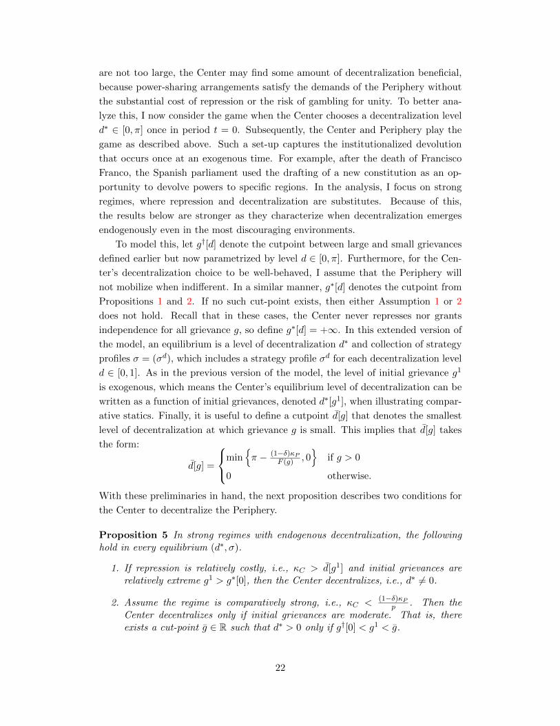
the Center to decentralize the Periphery.
Proposition 5 In strong regimes with endogenous decentralization, the followinghold in every equilibrium (d∗, σ).
1. If repression is relatively costly, i.e., κC > d[g1] and initial grievances arerelatively extreme g1 > g∗[0], then the Center decentralizes, i.e., d∗ 6= 0.
2. Assume the regime is comparatively strong, i.e., κC < (1−δ)κPp . Then the
Center decentralizes only if initial grievances are moderate. That is, thereexists a cut-point g ∈ R such that d∗ > 0 only if g†[0] < g1 < g.
22

Figure 6: Initial grievances, g1, and equilibrium decentralization, d∗[g1].
æ æ æ æ æ æ æ æ æ æ æ æ æ æ æ æ æ æ
æ
æ
æ
æ
æ
æ
æ
æ
æ
æ
æ
æ
æ
æ
æ
æ
æ
ææ
ææ
ææ
ææ
æ æ æ æ æ æ æ æ
10
20
30
40
50
EquilibriumDecentralization
10 20 30 40 50
Initial Grievance
Caption: For each initial grievance g1, the Center’s optimal decentralization level is computedwhen the parameters are as follows: π = 100, κC = 50, κP = 300, and δ = 0.95, ψ = 25, andF (g) = 1− 1
0.01g+1. In this case, g†[0] = 17.
In words, Proposition 5 details sufficient and necessary conditions for decentral-
ization to arise endogenously. The first result is a sufficient condition and says that
when the Center expects to enter into a repressive relationship with the Periphery
absent decentralization, i.e., g1 > g∗[0], and this repression is costly, i.e., κC > d[g1],
then it decentralizes control over the region. This sufficient condition is particularly
important because it guarantees that central governments will decentralize power to
an aggrieved Periphery even with cost-effective repression. In contrast, the second
is a necessary condition, and it says that the Center only decentralizes to minority
groups with moderate grievances.
To better understand this last result, Figure 6 graphs the Center’s equilibrium
level of decentralization, d∗[g1]. As stated in the proposition, decentralization only
occurs when the Periphery has moderate grievances. When g1 is small, there is no
need to decentralize as the Periphery will never mobilize. When g1 is quite large,
the amount of decentralization the Periphery demands is unpalatable to the Center,
and repression is a more cost-effective policy response. In contrast, when g1 is
moderate, the Center finds some level decentralization preferable, and it appeases
the Periphery with small levels of power sharing.
To see why the Center chooses these specific decentralization levels, Figure 7
graphs the Center’s equilibrium continuation value as a function of decentralization
when the game begins with four different regional grievance levels. Each of these
initial values potentially represents a different type of regional group with varying
historical grievances. Consider the group in Figure 7(a). Here, g1 ≤ g†[0], so the
23
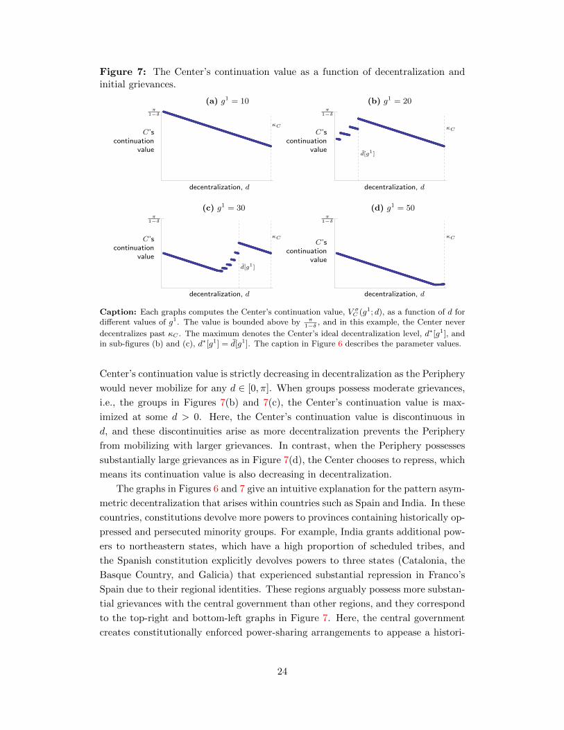
Figure 7: The Center’s continuation value as a function of decentralization andinitial grievances.
æææææææææææææææææææææææææææææææææææææææææææææææææææææææææææææææææææææææææææææææææææææææææææææææææææææææææææææææææææææææææææææææææææææææææææææææææææææææææææææææææææææææææææææææææææææææææææææææææææææææææææææææææææææææææææææææææææææææææææææææææææææææææææææææææææææææææææææææææææææææææææææææææææææææææææææææææææææææææææææææææææææææææææææææææææææææææææææææææææææææææææææææææææææææææææææææææææææææææææææææææææææææææææææææææææææææææææææææææææææææææææææææææææææææææææææææææææææææææææææææææææææææææææææææææææææ
æææææææææææææææææ
ææææææææææææææææææææææææææææææææææææææææææææ
æææææææææææææææææææææææææææææææææææææææ
æææææææææææææææææææææææææææææææææææææææææææææææææææææææææææææææææææææææææææææææææææææææææææææææææææææææææææææææææææææææææææææææææææææææææææææææææææææææææææææææææææææææææææææææææææææææææææææææææææææææææææææææææææææææææææææææææææææææææææææææææææææææææææææææææææææææææææææææææææææææææææææææææææææææææææææææææææææææææææææææææææææææææææææææææææææææææææææææææææææææææææææææææææææææææææææææææææææææææææææææææ
ææææææææææææææææææææææææææææææææææææææææææææææææææææææææææææææææææææææææææææææææææææææææææææææææææææææææææææææææææææææææææææææææææææææææææææææææææææææææææææææææææææææææææææææææææææææææææææææææææææææææææææææææææææææææææææææææææææææææææææææææææææææææææææææææææææææææææææææææææ
æææææææææææææææææææææ
ææææææææææææææææææææ
ææææææææææææææææææ
æææææææææææææææææ
æææææææææææææææææææææææææææææææææææææææææææææææææææææææææææææææææææææææææææææææææææææææææææææææææææææææææææææææææææææææææææææææææææææææææææææææææææææææ æææææææææææææææææææææææææææææææææææææææææææææææææææææææææææææææææææææææææææææææææææææææææææææææææææææææææææææææææææææææææææææææææææææææææææææææææææææææææææææææææææææææææææææææææææææææææææææææææææææææææææææææææææææææææææææææææææææææææææææææææææææææææææææææææææææææææææææææææææææææææææææææææææææææææææææææææææææææææææææææææææææææææææææææææææææææææææææææææææææææææææææææææææææææææææææææææææææææææææææææææææææææææææææææææææææææææææææææææææææææææææææææææææææææææææææææææææææææææææææææææææææææææææææææææææææ
(c) g1 = 30
C’scontinuation
value
π1−δ
decentralization, d
d[g1]
κC
(a) g1 = 10
C’scontinuation
value
π1−δ
decentralization, d
κC
(b) g1 = 20
C’scontinuation
value
π1−δ
decentralization, d
κC
d[g1]
(d) g1 = 50
C’scontinuation
value
π1−δ
decentralization, d
κC
Caption: Each graphs computes the Center’s continuation value, V σC (g1; d), as a function of d fordifferent values of g1. The value is bounded above by π
1−δ , and in this example, the Center never
decentralizes past κC . The maximum denotes the Center’s ideal decentralization level, d∗[g1], andin sub-figures (b) and (c), d∗[g1] = d[g1]. The caption in Figure 6 describes the parameter values.
Center’s continuation value is strictly decreasing in decentralization as the Periphery
would never mobilize for any d ∈ [0, π]. When groups possess moderate grievances,
i.e., the groups in Figures 7(b) and 7(c), the Center’s continuation value is max-
imized at some d > 0. Here, the Center’s continuation value is discontinuous in
d, and these discontinuities arise as more decentralization prevents the Periphery
from mobilizing with larger grievances. In contrast, when the Periphery possesses
substantially large grievances as in Figure 7(d), the Center chooses to repress, which
means its continuation value is also decreasing in decentralization.
The graphs in Figures 6 and 7 give an intuitive explanation for the pattern asym-
metric decentralization that arises within countries such as Spain and India. In these
countries, constitutions devolve more powers to provinces containing historically op-
pressed and persecuted minority groups. For example, India grants additional pow-
ers to northeastern states, which have a high proportion of scheduled tribes, and
the Spanish constitution explicitly devolves powers to three states (Catalonia, the
Basque Country, and Galicia) that experienced substantial repression in Franco’s
Spain due to their regional identities. These regions arguably possess more substan-
tial grievances with the central government than other regions, and they correspond
to the top-right and bottom-left graphs in Figure 7. Here, the central government
creates constitutionally enforced power-sharing arrangements to appease a histori-
24

cally aggrieved population that may seek independence without such concessions.
In contrast, less historically repressed regions or populaces without strong regional
identities were not granted the same considerations.
In Figure 7, when the Center decentralizes (top-right and bottom-left graphs),
it chooses a level d∗ that deters the Periphery from mobilizing in the subsequent
interaction. As the following proposition points out, however, this not a general
property of the model.
Proposition 6 If repression is not too costly, i.e., κC < max{π2 , π − d[g1]
}, then
the following hold
1. If the Center decentralizes, i.e, d∗ > 0, in equilibrium (d∗, σ), then it neitherrepresses nor grants independence along the subsequent path of play.
2. There exists a non-empty, open set of parameters in which the governmentdecentralizes (d∗ > 0) and neither repression nor mobilization occurs alongthe path of play in the unique equilibrium (d∗, σ).
3. There exists a non-empty, open set of parameters in which the governmentdecentralizes (d∗ > 0) and mobilization (but no repression) occurs along thepath of play in the unique equilibrium.
In words, Proposition 6(1) says that, assuming κC is small enough, if the Center
decentralizes, then it refrains from repressing the minority group or granting it inde-
pendence in the subsequent interaction.18 Propositions 6(2) and 6(3) are possibility
results describing these accommodative relationships. The former illustrates that
the Center may completely appease the secessionist threat with decentralization,
resulting in a peaceful relationship. In contrast, the latter demonstrates that the
Center may decentralize to a positive degree but not enough to completely deter
mobilization in the subsequent interaction. Such a situation arises when the Cen-
ter does not write a permanent power-sharing agreement with a Periphery whose
grievances, and hence capacity for mobilization, will deteriorate quickly over time.19
In these cases, the Center’s optimal strategy is to decentralize and appease only
moderately aggrieved groups although the Periphery is mobilizing with probability
one along the subsequent path of play. This means that mobilization and secession
can still occur after the Center optimally decentralizes.
Proposition 6 carries an important implication for bargaining theories of civil
war. Essentially, war (or mobilization) occurs with positive probability in this model
even though there is complete information and no commitment problem. Like previ-
ous models, this dynamic requires a sudden decrease in the Periphery’s probability
18Proposition 6(1) also guarantees an optimal d∗ exists. Specifically, any d∗ > 0 must makethe Periphery indifferent between mobilizing and not at some grievance g > g†[0] and g < g1.Thus, conditional on beginning at g1, the Center will maximizes its continuation value from neverrepressing or granting independence over finite set of decentralization levels.
19In other words, the result requires a convexity in F .
25

of winning, but conflict still persists with credible commitment, unlike other models
where credible commitment prevents conflict (e.g. Acemoglu and Robinson 2005;
Fearon 2004; Powell 2006). This difference emerges because the Center chooses a
level of decentralization that appeases moderately aggrieved groups tomorrow, but
today, it gambles that intense grievances will depreciate without successful secession.
The result in Proposition 6(3) does require that the Center decentralizes only
at the beginning of the game. More substantively, this assumption implies that the
timing of the central government’s decision is exogenous, but the government still
optimally chooses the degree of local autonomy. If the Center can also choose the
timing of decentralization in the equilibrium from Proposition 6(3), then it’s optimal
strategy would be to delay decentralization, risk several periods of minority unrest
by abstaining from repression, and then decentralize only after minority grievances
have depreciated to smaller levels. Such a setup is beyond the scope of the paper,
however. If the timing of decentralization is endogenous, then this suggests that the
issue of decentralization can be revisited, that is, the Center may choose more or
less decentralization in the future. In this case, decentralization becomes temporary
commitment, which does not reflect the situation in many federalist countries with
constitutionally protected regional powers.
5 Conclusion
This paper investigates the decentralization dilemma and offers an explanation as
to why decentralization can both encourage secessionist conflict and contribute to
a lasting peace in multiethnic societies. The theory centers around the dynamics
of intergroup tensions and their effects on the long-term strategies of governments
and minority groups. One effect is obvious. As the degree of regional autonomy
increases, minority groups with smaller grievances are less likely to mobilize for
secession. Because of this, decentralization decreases the time required for minority
grievances to reach peaceful levels, thereby attenuating the security costs associated
with the Center’s strategy to gamble for unity. This creates a second effect, where
larger levels of decentralization incentivize the government to avoid repression and
to lay the foundation for a lasting peace by tolerating minority unrest in the interim.
The theory highlights the interaction of a minority’s latent grievance and the
majority’s long-run repression/decentralization strategy in determining a country’s
evolution toward or away from peace. This is particularly important because the
interaction generates intricate relationships among grievance, repression and mi-
nority mobilization, hindering the efforts to uncover monotonic or even quadratic
effects. This suggests that a more structural or theoretically informed empirical
analysis is required to analyze relationships between grievances and observable ac-
tions. Such an endeavor might allow grievances to be estimated as an unobserved
26

state variable in a structural model. Likewise, the interaction between grievances
and the Center’s strategy induces non-monotonic relationships between decentral-
ization and the probability of national unity or secession. The analysis also generates
a testable implication that a U-shaped relationship exits between decentralization
and the probability of secession in strong regimes.
Besides a focus on latent grievances, the model raises several promising avenues
for future research and improvement, two of which appear particularly pressing.
First the analysis assumes that decentralization occurs only once at the beginning
of the game, and such an assumption appears restrictive. For example, the United
Kingdom devolved several powers to Scotland and Wales in 1998 after decades of
stasis. To better capture this dynamic, future work may endogenize the timing of
decentralization and allow the Center to repeatedly revisit the issue. In addition, in
the model, central governments create decentralized institutions with considerable
speed and precision; however, this may not be the case. Instead, it may take several
periods before decentralization can be fully implemented or governments may choose
decentralization levels from a far more coarse set. In this case, decentralization is
more like a hatchet, rather than a scalpel, and the analysis could include periods of
institutional friction in which decentralization becomes gradually implemented.
A Continuation Values and Expected Utilities
Let Vi denote i’s continuation value when the game begins in a period where the
Periphery controls the region, i.e., in some state x = (P, g). These values are
independent of σ and take the form VC = 0 and VP =πPP1−δ . Let UσC(r; g) and
UσP (m; g) denote the Center and Periphery’s dynamic payoffs from choosing r ∈{∅, 0, 1} and m ∈ {0, 1} in state x = (C, g), respectively, when actors subsequently
play according to profile σ. For the Center, UσC(r; g) takes the following form:
UσC(r; g) =
0 if = ∅
πCC − κC + δV σC (g + 1) if r = 1
−σP (g)F (g)ψ + (1− σP (g)F (g))(πCC + δV σ
C (g − 1))
if r = 0.
For the Periphery, UσP (m; g) denotes the its dynamic payoff conditional on having
reached its decision node, i.e., the Center chooses r = 0, in state x = (C, g). Thus,
UσP (m; g) takes the form
UσP (m; g) =
−κC + F (g)VP + (1− F (g))(πCP + δV σ
P (g − 1))
if m = 1
πCP + δV σP (g − 1) if m = 0.
(1)
With this notation in hand, the next definition states the equilibrium conditions.
27

Definition 1 Strategy profile σ is an equilibrium if the following hold:
σC(r; g) > 0 =⇒ UσC(r; g) ≥ UσC(r′; g),
σP (g) > 0 =⇒ UσP (1; g) ≥ UσC(0; g), and
σP (g) < 1 =⇒ UσP (0; g) ≥ UσC(1; g)
for all grievance g and polices r, r′ ∈ {∅, 0, 1}.
Notice that for some grievance g, the Center’s continuation value, V σC (g), takes
the form
V σC (g) =
∑r∈{∅,0,1}
σ(r; g)UσC(r; g).
Thus, if σ is an equilibrium and σ(r; g) > 0 for some grievance g and action r ∈{∅, 0, 1}, then V σ
C (g) = UσC(r; g) or else C has a deviation by playing some r′ ∈{∅, 0, 1}.
B Proof of Lemma 1
I restate and then prove the lemma. As discussed in Section 3, I maintain the generic
assumption that κP > F(g†) πPP−πCP
1−δ .
Lemma 1 If grievances are small, then the Periphery never mobilizes, and theCenter neither represses nor grants independence. That is, g ≤ g† implies σP (g) = 0and σC(0; g) = 1 in every equilibrium σ.
Proof. We first prove that g ≤ g† implies the Periphery does not mobilize with
positive probability. To see this, suppose σP (g) > 0 for some g ≤ g† and equilibrium
σ. To rule out profitable deviations, we require UσP (1; g) ≥ UσP (0; g). By Equation
1, this equivalent to
κP ≤ F (g)[VP − πCP − δV σ
P (g − 1)].
Now V σP (g − 1) ≥ πCP
1−δ for any equilibrium σ. To derive this lower bound, note that
when P mobilizes with probability zero in all future periods, its per-period payoff
is πCP , which is independent of σC . Thus, it cannot be that V σP (g − 1) <
πCP1−δ , as P
would profitably deviate by never mobilizing in all future periods. Combining these
two inequalities, we have
κP ≤ F (g)[VP − πCP − δV σ
P (g − 1)]
≤ F (g)
[VP −
πCP1− δ
]= F (g)
πPP − πCP1− δ
.
28

Thus, κC ≤ F (g)πPP−π
CP
1−δ , but this contradicts the assumption that g ≤ g†.With this result established, we prove that g ≤ g† implies the Center does
not repress or grant independence with positive probability. To see this, suppose
σC(r; g) > 0 for some g ≤ g†, r 6= 0, and equilibrium σ. There are two cases.
Case 1: r = 1, repression. Then, C’s expected utility is
UσC(1; g) = πC − κC + δV σC (g + 1)
≤ πC − κC + δπCC
1− δ
<πCC
1− δ.
However,πCC1−δ is C’s continuation value if it takes action r = 0 in all future periods
because grievances will never increase and the previous result establishes that P will
never mobilize with positive probability along the subsequent path of play. Hence,
taking action r = 0 in all future periods is a profitable deviation, a contradiction.
Case 2: r = ∅, independence. Then, C’s expected utility is
UσC(∅; g) = 0
<πCC
1− δ.
As in Case 1, this inequality implies taking action r = 0 in all future periods is a
profitable deviation, a contradiction.
C Preliminary Results
Before proving the main result, we prove a series of lemmas which hold across
regime type and do not depend on Assumptions 1 or 2 unless explicitly stated.
These lemmas are fairly technical, so they have been relegated to the Appendix.
Let the function VC : N→ R denote C’s continuation value from beginning the
game at state (C, g) and continuing to play r = 0 for all future periods while P
mobilizes if and only if g > g†. Specifically, this means VC(g) takes the form
VC(g) =
πCC1−δ if g ≤ g†
−F (g)ψ + (1− F (g))(πCC + δVC(g − 1)) if g > g†.
Figure 8 illustrates an example of VC , and we now establish several properties of VC
which are essential to the subsequent analysis.
Lemma 2 1. VC(g) >−F (g)ψ+(1−F (g))πCC
1−(1−F (g))δ for all g such that F (g) > 0.
29

æ æ æ æ æ
æ
æ
æ
æ
æ
æ
æ
æ
æ
æ
æ
æ
æ
æ
æ
æ
æ
ææ
ææ
ææ
ææ æ æ æ æ æ æ æ æ æ æ æ æ æ æ æ æ æ æ æ æ æ æ æ æ æ æ æ æ æ æ æ
max G1g
Π1-∆
V�
C
Figure 8: Graph of VC . To produce the figure, the parameters take values πCC =100, κC = 25, κP = 75, ψ = 400, and δ = 0.95. In addition, F (g) = 1− 1
0.01g+1 .
2. VC(g − 1) > VC(g) for all g > g†.
3. If the Periphery values independence, then limg→∞ VC(g) =−pψ+(1−p)πCC
1−(1−p)δ .
Proof. To show (1), consider some g such that F (g) > 0 and F (g′) = 0 for all g′ < g.
Such a g exists because F (0) = 0 and limg→∞ F (g) = p > 0. Then we have
VC(g) = −F (g)ψ + (1− F (g))
(πCC + δ
πCC1− δ
)= (1− (1− F (g))δ)
−F (g)ψ + (1− F (g))πCC1− (1− F (g))δ
+ (1− F (g))δπCC
1− δ
>−F (g)ψ + (1− F (g))πCC
1− (1− F (g))δ.
Above, the strict inequality follows because (a) F (g) > 0 and (b) F is strictly
increasing with limit p > 0 imply that F (g) ∈ (0, p).
For induction, consider some g such that F (g) > 0 and F (g − 1) > 0. Suppose
the inequality holds for all g′ < g such that F (g′) > 0. Then we have
VC(g) = −F (g)ψ + (1− F (g))(πCC + δVC(g − 1))
> −F (g)ψ + (1− F (g))
(πCC + δ
−F (g − 1)ψ + (1− F (g − 1))πCC1− (1− F (g − 1))δ
)≥ −F (g)ψ + (1− F (g))
(πCC + δ
−F (g)ψ + (1− F (g))πCC1− (1− F (g))δ
)=−F (g)ψ + (1− F (g))πCC
1− (1− F (g))δ,
30

where the third line follows because the fraction−F (g)ψ+(1−F (g))πCC
1−(1−F (g))δ is decreasing in
F (g).
To show (2), note that it must hold when g = g† + 1 because ψ > 0 and
g > g† implies F (g) > 0. Now consider some g > g† + 1. For induction, suppose
VC(g′ − 1) > VC(g′) for all g′ such that g† < g′ < g. Because g > g†, we have
VC(g) = −F (g)ψ + (1− F (g))(πCC + δVC(g − 1))
≤ −F (g − 1)ψ + (1− F (g − 1))(πCC + δVC(g − 1))
< −F (g − 1)ψ + (1− F (g − 1))(πCC + δVC(g − 2))
= VC(g − 1),
where the second line follows because
VC(g) >−F (g)ψ + (1− F (g))πCC
1− (1− F (g))δ≥ −ψ
and F (g) is increasing in g.
To prove (3), consider a sequence {gn}∞n=1 such that limn→∞ gn =∞ and gn <
gn+1. Then the sequence{VC(gn)
}∞n=1
is weakly decreasing because it is strictly
decreasing gn+1 > g† and constant when gn+1 < g†. In addition,{VC(gn)
}∞n=1
is
bounded below because C’s payoffs are finite and C discounts with rate δ < 1. Thus,{VC(gn)
}∞n=1
has a limit, call it L. If the Periphery does value independence, the
we have
L = limn→∞
VC(gn)
= limn→∞
F (gn)(−ψ) + limn→∞
(1− F (gn))(πCC + δVC(gn − 1))
= −pψ + (1− p)(πCC + δL
),
which implies L =−pψ+(1−p)πCC
1−(1−p)δ .
Lemma 3 For all grievances g, V σC (g) ≥ VC(g) in every equilibrium σ.
Proof. To see this, suppose not. That is, suppose there exist grievance g and equi-
librium σ such that V σC (g) < VC(g). Then by the construction of VC and Lemma 1,
g > g†, or else V σC (g) =
πCC1−δ = VC .
Next consider a deviation for C, labeled σ′C , such that σ′C(0; g′) = 1 for all
g′ ≤ g. I now demonstrate that V σ′C (g) ≥ VC(g), where σ′ = (σ′C , σP ), which implies
σ′C is a profitable deviation because VC(g) > V σC (g) by supposition.
The proof is by induction. The inequality, V σ′C (g′) ≥ VC(g′), holds when g′ ≤ g†
by the construction of VC and Lemma 1. Now consider some g′ > g† and suppose
31

V σ′C (g′′) ≥ VC(g′′) for all g′′ < g. Then we have
V σ′C (g′) = −σP (g)F (g)ψ + (1− σP (g′)F (g′))
(πCC + δV σ′
C (g′ − 1))
≥ −σP (g′)F (g′)ψ + (1− σP (g′)F (g′))(πCC + δVC(g′ − 1)
)≥ −F (g′)ψ + (1− F (g′))
(πCC + δVC(g′ − 1)
)= VC(g′).
Hence, V σ′C (g) ≥ VC(g) as required.
Lemma 4 If σC(1; g) > 0 and σC(0; g + 1) = 1 for some grievance g, then σP (g +1) < 1 in every equilibrium σ.
Proof. Suppose not. Then there exists a g such that σC(1; g) > 1, σC(0; g + 1) = 1
and σP (g + 1) = 1 in equilibrium σ. We can write V σC (g + 1) as
V σC (g + 1) = −F (g + 1)ψ − (1− F (g + 1))
(πCC + δV σ
C (g))
= −F (g + 1)ψ − (1− F (g + 1))(πCC + δUσC(1; g)
)= −F (g + 1)ψ − (1− F (g + 1))
(πCC + δ
(πCC − κC + δV σ
C (g + 1))).
Solving reveals that
V σC (g + 1) =
(1− F (g + 1))(π(1 + δ)− δκC)− F (g + 1)ψ
1− (1− F (g + 1))δ2.
By Lemma 3, V σC (g + 1) ≥ VC(g + 1). By Lemma 2(1),
VC(g) >(1− F (g + 1))πCC − F (g + 1)ψ
1− (1− F (g + 1)δ).
Stringing these two inequalities together,
V σC (g + 1) >
(1− F (g + 1))πCC − F (g + 1)ψ
1− (1− F (g + 1)δ).
Substituting the closed form solution for V σC (g + 1) into the inequality above and
solving for κC reveals that
κC <F (g + 1)(πCC + ψ(1− δ))
1− (1− F (g + 1))δ.
To derive a contradiction, consider a deviation in which C plays r = 1 with
probability 1 in all future periods beginning at grievance g + 1. This is a profitable
32

deviation if and only if
V σC (g + 1) <
πCC − κC1− δ
⇐⇒ κC <F (g + 1)(πCC + ψ(1− δ))
1− (1− F (g + 1))δ.
However, κC <F (g+1)(πCC+ψ(1−δ))
1−(1−F (g+1))δ as shown above. Hence, C can profitably deviate
by always repressing.
Lemma 5 Consider some g > g† and equilibrium σ. If (a) σC(0; g − 1) = 1 orσC(0; g) = 1 and (b) σC(∅; g′) = 0 for all g′ < g, then σP (g) = 1.
Proof. Suppose not. That is, consider some equilibrium σ and grievance g > g† such
that
(a) σC(0; g − 1) = 1 or σC(0; g) = 1,
(b) σC(∅; g′) = 0 for all g′ < g, and
(c) σP (g) < 1.
Because σ is an equilibrium, we require UσP (0; g) ≥ UσP (1; g) to rule out profitable
deviations, which is equivalent to
κP ≥ F (g)[VP − πCP − δV σ
P (g − 1)].
Because σC(0; g − 1) = 1 or σC(0; g) = 1, the path of play will never reach a
grievance larger than g. Because σC(∅; g′) = 0 for all g′ ≤ g, the Center will never
grant independence along the subsequent path of play. Recall that when the C
represses, P stage payoff is πCP , which is its payoff if it chooses not to mobilize, and
even if C does repress with positive probability at some g′ < g, the subsequent path
of play will still never reach a grievance larger than g. Then g > g† implies V σP (g−1)
is bounded above byF (g)VP + (1− F (g))πCP − κP
1− (1− F (g))δ,
which is P ’s payoff if its grievance never depreciates along the path of play, C never
represses, and P always mobilizes. Combining these two inequalities, we require
κP ≥ F (g)[VP − πCP − δV σ
P (g − 1)]
≥ F (g)
[VP − πCP − δ
F (g)VP + (1− F (g))πCP − κP1− (1− F (g))δ
].
Solving for κP implies
κP ≥ F (g)πPP − πCP
1− δ,
that is, g ≤ g†. But this contradicts the assumption g > g†.
33

D Equilibrium behavior with moderate grievances
This section characterizes the model’s equilibria for moderate grievances. Essen-
tially, the main result states that the Center neither represses nor grants indepen-
dence with moderate grievances, and this characterization is constant across regime
type. To define moderate grievances, we introduce the cut-point g∗. Let g∗ ∈ R be
a cut-point that solves
g < g∗ =⇒ VC(g) > max
{πCC − κC
1− δ, 0
}, and
g > g∗ =⇒ VC(g) < max
{πCC − κC
1− δ, 0
}.
(2)
Lemma 6 The cut-point g∗ solving Equation 2 exists if and only if the Peripheryvalues independence (Assumption 1) and secession is costly (Assumption 2).
Proof. For necessity, suppose Assumptions 1 and 2 hold. Then Lemma 2 and As-
sumption 1 imply that VC(g) is weakly decreasing in g and converges to
limg→∞
VC(g) =−pψ + (1− p)πCC
1− (1− p)δ.
Because VC(g) =πCC1−δ > 0 for all g ≤ g† and VC(g) is strictly decreasing in g when
g > g†, we require
−pψ + (1− p)πCC1− (1− p)δ
< max
{πCC − κC
1− δ, 0
}, (3)
by the continuity of VC(g).
We now demonstrate that the inequality in Equation 3 holds in strong regimes;
the argument for weak regimes is identical. Suppose πCC − κC > 0. Then Equation
3 reduces to−pψ + (1− p)πCC
1− (1− p)δ<πCC − κC
1− δ,
which is equivalent to
ψ >(1− δ)κC − p(πCC − δκC)
p(1− δ).
Because πCC − κC > 0, Assumption 2 reduces to
ψ > min
{πCC (1− p)
p,(1− δ)κC − p(πCC − δκC)
p(1− δ)
}=
(1− δ)κC − p(πCC − δκC)
p(1− δ).
34

Thus, the inequality in Equation 3 holds, and therefore g∗ exists.
For sufficiency, suppose Assumption 1 does not hold, then g† does not exist. That
is, κP > F (g)πPP−π
CP
1−δ for all grievances g. Thus, VC(g) =πCC1−δ > max
{πCC−κC
1−δ , 0}
for all grievances g, and there cannot exist a real number g∗ ∈ R such that g > g∗
implies VC(g) < max{πCC−κC
1−δ , 0}
.
Now suppose Assumption 1 holds but not Assumption 2. Then Lemma 2 implies
that, for all g,
VC(g) ≥−pψ + (1− p)πCC
1− (1− p)δ
> max
{πCC − κC
1− δ, 0
},
where the last inequality follows because Assumption 2 does not hold. Thus,
there does not exist a real number g∗ ∈ R such that g > g∗ implies VC(g) <
max{πCC−κC
1−δ , 0}
.
We now prove that g < g∗ implies σC(0; g) = 1 in every equilibrium σ, that
is, the Center neither represses nor grants independence with moderate grievances.
The result requires three preliminary lemmas. Notice that if either Assumption 1
or 2 does not hold, VC(g) > max{πCC−κC
1−δ , 0}
for all g, and we can set g∗ = ∞ in
the subsequent results.
Lemma 7 If g < g∗, then σC(∅; g) = 0 in every equilibrium σ.
Proof. By Lemma 1, the result holds if g ≤ g†. So consider g > g† and suppose,
contrary to the hypothesis, that σC(∅; g) > 0 for some grievance g < g∗ and some
equilibrium σ. Then V σC (g) = UσC(∅; g) = 0. This contradicts Lemma 3 because
VC(g) > 0 = V σC (g) if g < g∗.
Lemma 8 In strong regimes, the Center does not grant independence with positiveprobability, i.e., σC(∅; g) = 0 for all g in every equilibrium σ.
Proof. The result holds for g ≤ g† by Lemma 1. Suppose the result does not hold
for some g > g†. Then σC(∅; g) > 0 implies UσC(∅; g) = 0, but C’s dynamic payoff
of repressing at g is
UσC(1; g) = πCC − κC + δV σC (g + 1).
Then V σC (g + 1) ≥ 0 or else C can profitably deviate at g + 1 by granting indepen-
dence. But this implies UσC(1; g) ≥ πCC − κC > 0, so C has a one-shot deviation at
g by repressing, a contradiction.
35
Lemma 9 For all g, σ(r; g) > 0 implies σ(∅; g + 1) = 0 in every equilibrium σ.
Proof. By Lemma 8, the statement is vacuously true in strong regimes. Thus,
consider a weak regime, i.e, assume π − κC < 0. Suppose σC(r; g) > 0 for some g
and σC(∅; g + 1) > 0. Then
V σC (g) = UσC(r; g)
= π − κC + δV σC (g + 1)
= π − κC + δUσC(∅; g)
= π − κC < 0,
but this means C can profitably deviate at g by granting independence, i.e., σ is
not an equilibrium.
Lemma 10 Fix an equilibrium σ. Then there does not exist a g < g∗ such thatσC(1; g′) > 0 for all g′ ≥ g.
Proof. Suppose not and consider such a g < g∗ where σC(1; g′) > 0 for all g′ ≥ g in
equilibrium σ. Then
V σC (g) = UσC(1; g)
= πCC − κC + δV σC (g + 1).
Because VC(g′) = UσC(r; g′) for all g′ such that σC(r; g′) > 0, similar substitutions
imply V σC (g) =
πCC−κC1−δ . However, g < g∗ implies
VC(g) >πCC − κC
1− δ= V σ
C (g),
by Equations 2. However, VC(g) > V σC (g) contradicts Lemma 3.
With these lemmas in hand, we now state the main result of the section.
Lemma 11 If g < g∗, then σ(0, g) = 1 in every equilibrium σ.
Proof. The claim holds if g ≤ g† by Lemma 1. So consider g > g† such that g < g∗
where σC(0; g) < 1. By Lemma 7, σC(1; g) > 0. Furthermore, C represses with
positive probability for at most some finite k periods by Lemma 10. That is, there
exists a g+ such that σC(1; g′) > 0 for g′ = g, ..., g+ and σC(1; g+ + 1) = 0. By
Lemma 9, this implies σC(0; g+ + 1) = 1. In addition, Lemmas 1 and 9 imply
σC(∅; g′) = 0 for all g′ < g+. Thus, Lemma 5 and σC(1; g+ + 1) = 0 imply P
36

mobilizes at g+ + 1 with probability 1. However, σC(1; g+) > 0, σC(0; g+ + 1) = 1,
and σP (g+ + 1) = 1 contradict Lemma 4.
Almost as an immediate corollary, the following lemma characterizes P ’s equi-
librium strategy for moderate grievances. It only consider the generic case in which
g∗ is not an integer.
Lemma 12 If g > g† and g ≤ bg∗ + 1c, then σP (g) = 1 in every equilibrium σ.
Proof. Because g ≤ bg∗ + 1c, Lemma 11 implies σC(0; g′) = 1 for all g′ < bg∗ + 1c.Then Lemma 5 implies σP (g) = 1.
E Proof of Proposition 1
This section proves Proposition 1. Notice that the previous section characterizes
equilibrium behavior for moderate grievances, i.e., g < g∗. We now character-
ize equilibrium behavior for large grievances (g > g∗) and then restate and prove
Proposition 1. Due to the result in Lemma 6, we maintain Assumptions 1 and 2
throughout, or else no g∗ characterizing Equation 2 exists. As before, we consider
the generic case in which there does not exist g ∈ N0 such that VC(g) =πCC−κC
1−δ ,
that is, g∗ is not an integer.
Lemma 13 In strong regimes, σC(1; bg∗ + 1c) = 1 and σC(1; g) > 0 for all g > g∗
in every equilibrium σ.
Proof. The proof is by induction. First, we demonstrate that σC(1; bg∗ + 1c) = 1.
To see this, suppose σC(1; bg∗+1c) < 1. Then Lemma 8 implies σC(0; bg∗+1c) > 0.
By Lemmas 11 and 12,
UσC(0; bg∗ + 1c) = VC(bg∗ + 1c)
<πCC − κC
1− δ,
because bg∗+1c > g∗. But this means C can profitably deviate at grievance bg∗+1cby repressing for an infinite number of periods, a contradiction.
For induction, consider some g > bg∗ + 1c and assume σC(1; g − 1) > 0. To
derive a contradiction, assume σC(1; g) = 0. By Lemma 8, σC(0; g) = 1. Likewise,
Lemma 8 guarantees C does not grant independence in any equilibrium, so Lemma
5 implies P mobilizes at g with probability 1. But then this contradicts Lemma
4.
37

Lemma 14 In strong regimes, g > g∗ implies V σC (g) =
πCC−κC1−δ in every equilibrium
σ.
Proof. If g > g∗, then Lemma 13 implies σC(1; g′) > 0 for all g′ ≥ g. The remainder
of the proof follows from an almost identical argument as the one in Lemma 10.
Lemma 15 In strong regimes, g > g∗ and σC(0; g) > 0 imply σP (g) < 1 in everyequilibrium σ.
Proof. Suppose not. Then there exists g > g∗ such that σC(0; g) > 0 and σP (g) = 1.
Because σC(0; g) > 0, Lemma 13 implies g − 1 ≥ bg∗ + 1c. Likewise, σC(1; g) > 0
by Lemma 13, so it must be the case that UσC(0; g) = UσC(1; g). Then we have
UσC(0; g) = UσC(1; g) ⇐⇒ −F (g)ψ + (1− F (g))(πCC + δV σC (g − 1)) = π − κC + δV σ
C (g + 1)
⇐⇒ −F (g)ψ + (1− F (g))
(πCC + δ
π − κC1− δ
)=π − κC1− δ
⇐⇒ κC =F (g)(πCC + (1− δ)ψ)
1(1− F (g))δ,
where we use Lemma 14 and g− 1 ≥ bg∗+ 1c to substitute for values V σC (g− 1) and
V σC (g + 1).
Because σ is an equilibrium, we require UσC(1; g) = V σC (g) ≥ VC(g), by Lemma
3. Then Lemma 2(1) implies
UσC(1; g) >−F (g)ψ + (1− F (g))πCC
1− (1− F (g))δ⇐⇒
πCC − κC1− δ
>−F (g)ψ + (1− F (g))πCC
1− (1− F (g))δ
⇐⇒ κC <F (g)(πCC + (1− δ)ψ)
1(1− F (g))δ,
which establishes the desired contradiction.
Lemma 16 In strong regimes, there exists cut-point g ∈ R such that if g > g, thenσP (g) = 1 and σC(1; g) = 1 in every equilibrium σ.
Proof. The proof is constructive. Define g ∈ R to be a number that satisfies the
following implications:
g < g =⇒ κP > F (g)
[VP − πCP − δ
pVP + (1− p)πCP − κP1− (1− p)δ
], and
g > g =⇒ κP < F (g)
[VP − πCP − δ
pVP + (1− p)πCP − κP1− (1− p)δ
].
38
Such a g exists because F (g)[VP − πCP − δ
pVP+(1−p)πCP1−(1−p)δ
]is positive and strictly in-
creasing in g. Furthermore,
limg→∞
F (g)
[VP − πCP − δ
pVP + (1− p)πCP1− (1− p)δ
]= p
πPP − πCP1− δ
,
and Assumption 1 implies
κP < pπPP − πCP
1− δ.
We first show that σP (g) = 1 for g > g. Suppose not; then there exists g > g such
that σP (g) < 1. To rule out profitable deviations, we require UσP (0; g) ≥ UσP (1; g),
which is equivalent to
κC ≥ F (g)[VP − πCP − δV σ
C (g − 1)].
Because the Center never grants independence in strong regimes, V σC (g − 1) is
bounded above bypVP+(1−p)πCP−κP
1−(1−p)δ for the same reasons described in the proof of
Lemma 5. Combining these two inequalities gives us
κC ≥ F (g)[VP − πCP − δV σ
C (g − 1)]
≥ F (g)
[VP − πCP − δ
pVP + (1− p)πCP − κP1− (1− p)δ
],
but this implies g ≤ g, which is contradiction. Thus, σP (g) = 1. Then Lemma 13
and the contrapositive of Lemma 15 imply σC(1; g) = 1, as required.
Lemma 17 In strong regimes, if g > g∗, then σP (g) = 1 in every equilibrium σ.
Proof. Suppose not. Suppose there exists g such that g > g∗ and σP (g) < 1. Then
Lemma 16 implies that there exists grievance g+ ≥ g such that σP (g+) < 1 and
σP (g′) = σC(1; g′) = 1 for all g′ > g+. To rule out profitable deviations, we require
UσP (0; g+) ≥ UσP (1; g+). This implies
κP ≥ F (g+)[VP − πCP − δV σ
C (g+ − 1)].
Because P will never be able to mobilize at a larger grievance than g+ along the
path of play and C never grants independence, V σC (g+ − 1) is bounded above by
F (g+)VP + (1− F (g+))πCP − κP1− (1− F (g+)δ)
,
39

for the same reasons described in Lemma 5. Then we have
κP ≥ F (g+)[VP − πCP − δV σ
C (g+ − 1)]
≥ F (g+)
[VP − πCP − δ
F (g+)VP + (1− F (g+))πCP − κP1− (1− F (g+)δ)
]= F (g+)
πPP − πCP1− δ
,
which implies g+ ≤ g†. But g > g∗ > g† by construction. And g+ > g implies
g+ > g†, a contradiction.
We now restate and prove Proposition 1, which characterizes equilibria in strong
regimes.
Proposition 1 In strong regimes, there exists cutpoint g∗ ∈ R such that g∗ > g†
and the following hold in every equilibrium σ.
1. The Periphery mobilizes if and only if grievances are large, i.e., if g > g†, thenσP (g) = 1 and if g ≤ g†, then σP (g) = 0.
2. If g < g∗, then the Center neither represses nor grants independence, i.e.,σC(0; g) = 1, and grievances depreciate toward zero.
3. If g > g∗, then the Center uses repression, i.e., σC(1; g) = 1, perpetuatinggrievances toward positive infinity.
4. Secession occurs with positive probability along the path of play if and only ifgrievance are moderate, i.e., g† < g < g∗.
Proof. To see (1), note that, by Lemma 1, it suffices to show that if g > g†, then
P mobilizes with probability 1. Consider such a grievance g. There are two cases.
If g < g∗, then Lemma 12 implies σP (g) = 1. If g > g∗, then Lemma 17 implies
σP (g) = 1. The result in (2) follows immediately from Lemma 11. To see (3), note
that g > g∗ implies σP (g) = 1. Then Lemma 13 and the contrapositive of Lemma 15
imply σC(1; g) = 1, as required. The final result is a corollary of the first three.
F Proof of Proposition 2
This section proves Proposition 2. Notice that previous results characterizes equi-
librium behavior for moderate grievances, i.e., g < g∗. We now characterize equilib-
rium behavior for large grievances (g > g∗) and then restate and prove Proposition
2. Thus, we main Assumptions 1 and 2 throughout, or else no g∗ characterizing
Equation 2 exists. As before, we consider the generic case in which g∗ is not an
integer.
40
Lemma 18 Fix an equilibrium σ. In weak regimes, there does not exist a g suchthat σC(1; g′) > 0 for all g′ ≥ g.
Proof. The result follows from the inequality πCC−κC < 0 and the argument proving
Lemma 10.
Lemma 19 Consider g = bg∗+1c. In weak regimes, σC(0; g) = 0, and σC(∅; g) > 0in ever equilibrium σ.
Proof. First, we show that σC(0; g) = 0. If not, then V σC (g) = UσC(0; g) = VC(g),
by Lemmas 11 and 12. But then V σC (g) < 0 because g > g∗, so C can profitably
deviate by granting independence at g.
Second, we show that σC(1; g) < 1. To see this, suppose not, i.e., suppose
σC(1; g) = 1. By Lemma 18, there exists g+ > g such that σC(1; g+ + 1) = 0
and σC(1; g′) > 0 for all g′ = g, ..., g+. Then by Lemma 9, σC(∅; g′) = 0 for all
g′ = g, .., g+ + 1. By Lemma 11, σC(0; g′) = 1 for all g′ < g. Then Lemma 5 implies
σP (g+ + 1) = 1. However, σC(1; g+) > 0, σC(0; g+ + 1) = 1, and σP (g+ + 1) = 1
contradict Lemma 4. Thus, σC(1; g) < 1, which implies σC(∅; g) > 0 by the previous
paragraph.
Lemma 20 Consider g = bg∗ + 1c. In weak regimes, if F (g + 1)(πPP − πCP ) > κP ,then σP (g′) = 1 and σC(∅; g′) = 1 for all g′ > g∗ in every equilibrium σ.
Proof. First, we show that P mobilizes for all g′ > g∗. Lemma 12 demonstrates P
mobilizes at g = bg∗+1c. Now, P mobilizes at g′ > g if UσC(1; g′) > UσC(0; g′), which
is equivalent to
κC < F (g′)[VP − πCP − δV σ
P (g′ − 1)].
An upper bound on V σP (g′ − 1) is
πPP1−δ , which is the discounted sum of P ’s largest
per-period payoff. Combining these two inequalities implies P mobilizes when
F (g′)(πPP − πCP ) > κP , which holds because F (g + 1)(πPP − πCP ) > κP , and F is
increasing.
Second, I claim that σC(1; g′) = 0 for all g′ ≥ g. Suppose not. Then there exists
a g+ such that σC(1; g+) > 0 and σC(0; g+ + 1) = 1 by Lemmas 9 and 18. The
previous paragraph demonstrates that P mobilizes with probability 1 with grievance
g+ + 1. But this contradicts Lemma 4.
Third, I claim that σC(∅; g′) = 1 for all g′ > g∗. To see this, note that σC(1; g) =
0 and Lemma 19 imply σC(∅; g) = 1. For induction, consider some g′ such that
σC(∅; g′′) = 1 for all g′′ = g, ..., g′− 1. We show σC(∅; g′) = 1. To see this, suppose
not. By the previous paragraph, σC(1; g′) = 0, so σC(0; g) > 0. Because P mobilizes
41

at g′ > g, we have
UσC(0; g′) = −F (g′)ψ + (1− F (g′))πCC + δV σC (g′)
= −F (g′)ψ + (1− F (g′))πCC
< 0,
where the last inequality follows from g′ > g∗. But UσC(0; g′) < 0 means C can prof-
itably deviate at g′ by granting independence. Thus, σC(0; g′) = 0 in equilibrium,
which implies σC(∅; g′) = 1.
Before proving the last technical lemma of this section, consider the following
definitions. The set G ⊆ N0 is an absorbing set with respect to profile σ if once the
path of play enters state (C, g) such that g ∈ G, it never transitions to a state (C, g′)
such that g′ /∈ G with positive probability. The set G is an irreducible absorbing set
with respect to σ if G is an absorbing set with respect to σ and there does not exist
a proper subset G′ ( G such that G′ is an absorbing set with respect to σ.
Lemma 21 Consider an equilibrium σ and some g such that g > g∗. Then thefollowing hold:
1. beginning at grievance g, the path of play enters an irreducible absorbing setG,
2. maxG exists,
3. g∗ < minG, and
4. there exists g′ ∈ G such that σC(∅; g) > 0.
Proof. To prove (1), consider g > g∗ and two cases. If σC(1; g) = 0, then the path
of play enters the set {bg∗+ 1c, ..., g}, which is an absorbing set because σC(0; bg∗+
1c) = 0 by Lemma 19. So the set {bg∗+ 1c, ..., g} has a irreducible absorbing set, G.
If σC(1; g) > 0, then Lemma 18 imply there exists g+ > g such that σC(1; g′) > 0
for all g′ = g, ..., g+ and σC(1; g+ + 1) = 0 from Lemma 9. Then the path of play
enters the set {bg∗ + 1c, ..., g+ + 1}, which is an absorbing set as well.
The proof of (2) and (3) follow immediately from the existence of G and Lemmas
18 and 19, respectively.
To prove (4), suppose not. Suppose σC(∅; g′) = 0 for all g′ ∈ G. First, this
implies #G > 1. If #G = {g}, then C cannot be repressing with positive probability
at g, or else G is not absorbing. Also, if #G = {g} and σC(0; g) > 0, then F (g) = 1
and σP (g) = 1 or else the path of play would transition to g − 1 with positive
probability. In this case, UC(0; g) = −ψ < 0, but this means C has a profitable
deviation by granting independence at g.
Because G is an irreducible absorbing set, σC(1; maxG − 1) > 0, or else G \{maxG} would be absorbing as well. Furthermore, σC(1; maxG) = 0 or else the
42

path of play would transition with positive probability to maxG + 1. Because
σC(1; maxG − 1) > 0 and σC(1; maxG) = 0, Lemma 9 implies σC(0; maxG) = 1
Because the path of play never leaves G. and transitions to grievance g′ > maxGand C never grants independence along the path of play starting from maxG, then
σP (maxG) = 1, which follows from an identical argument as the one in Lemma 5.
However, this contradicts Lemma 4.
I now restate and prove Proposition 2.
Proposition 2 In weak regimes, there exists cutpoint g∗ ∈ R such that g∗ > g†,and the following hold in every equilibrium σ.
1. If g < g∗, then the Periphery mobilizes, i.e., σP (g) = 1, if and only if g > g†,and the Center neither represses nor grants independence, i.e., σC(0; g) = 1.
2. If g > g∗, then the path of play never transitions to grievance g′ < g∗, and theCenter grants independence with positive probability along the path of play.
3. If κP < F (bg∗ + 1c) (πPP − πCP ), then g > g∗ implies the Periphery mobilizes,i.e., σP (g) = 1, and the Center grants independence, i.e., σC(∅; g) = 1.
Proof. To prove (1) follows immediately from Lemmas 1, 11, and 12, which charac-
terize equilibrium behavior for grievances g < g∗. The proof of (2) follows immedi-
ately from Lemma 21, and the proof of (3) follows from Lemma 20.
G Proof of Proposition 3
I first prove an intermediary result.
Lemma 22 If κC > (1 + δ)πCC , then the Center never represses in any equilibriumσ, i.e., σC(1; g) = 0 for all grievances g.
Proof. To derive a contradiction, suppose the contrary. That is, suppose κC >
(1 + δ)πCC and the Center represses in equilibrium σ. Thus, the regime is weak, and
there exist some g such that σC(1; g) > 0. By Lemma 18, there exists g+ > g such
that σC(1; g+ + 1) = 0 and σC(1; g′) > 0 for all g′ = g, ..., g+. Then by Lemma 9,
σC(∅; g′) = 0 for all g′ = g+1, .., g+ +1. Hence, σC(0; g+ +1) = 1. We can compute
C’s continuation value at g+ as
V σC (g+) = UσC(1; g+)
= πCC − κC + δV σC (g+ + 1)
= πCC − κC + δ[σP (g+ + 1)
(−F (g+ + 1)ψ + (1− F (g+ + 1))(πCC + δV σ
C (g+))
+
(1− σP (g+ + 1))(πCC + δV σ
C (g+))].
43

Solving for V σC (g+) reveals that
V σC (g+) =
πCC (1 + (1− F (g+ + 1)σP (g+ + 1))δ)− κC − F (g+ + 1)σP (g+ + 1)δψ
1− (1− σP (g+ + 1)F (g+ + 1))δ2,
which is decreasing in σP (g+ + 1). Because σP (g+ + 1) ≥ 0, then
V σC (g+) ≤
πCC (1 + δ)− κC1− δ2
Thus, κC > (1+δ)πCC implies V σC (g+) < 0. But this implies C can profitably deviate
at g+ by granting independence and guaranteeing itself a payoff of zero.
Next, I restate and prove Proposition 3.
Proposition 3 In weak regimes, no equilibrium supports long-term repression, butthere exist equilibria that support cycles of repression and mobilization. Furthermore,if κC > (1 + δ)πCC , then the Center never represses with positive probability in everyequilibrium, i.e., σC(1; g) = 0 for every grievance g and equilibrium σ.
Proof. Lemma 18 proves the first claim, that is, there does not exist an equilibrium
σ and grievance g such that σC(1; g′) > 0 for all g′ ≥ g. In addition, Lemma 22
proves the final the claim, i.e., the necessary condition.
To prove the second claim, I construct an equilibrium. In this example, I assume
πCC = πPP = 1, and πCP = 0. In addition, κC = 1.2 and κP = .25. This implies that
the regimes is weak. Finally, δ = .9, ψ = 6, and F takes the form:
F (g) =
0 if g = 0
g700 + 33
175 if g ≥ 1 and g ≤ 8
.8 + γ(g) otherwise,
where γ is a strictly increasing function such that γ(9) = 0 and limg→∞ γ(g) = .2.
Thus, g† = 0, and g∗ can be any real number between 6 and 7, because VC(6) ≈ .33
and VC(7) ≈ −.15. By Proposition 2 and Lemma 12, the Periphery mobilizes with
probability one for all g ∈ {1, 2, ..., 7} and the Center neither represses nor grants
independence for all g ∈ {0, 1, 2, ..., 6}.Next, I claim that the Periphery mobilizes and the Center grants independence
with probability one for all g ≥ 9. From the logic in the proof of Lemma 20, it
suffices to show that
F (g)(πPP − πCP ) > κP ,
for all g ≥ 9. This inequality holds because F is strictly increasing and F (9)(πPP −πCP ) = .8, which is greater than κP = .25.
44

Next assume that σC(0; 8) = 1. We characterize mixing probabilities, σC(1; 7),
σC(∅; 7), and σP (8), such that the following hold:
σC(1; 7) + σC(∅; 7) = 1
UσC(1; 7) = UσC(∅; 7)
UσP (1; 8) = UσP (0; 8).
The first equation say the Center mixes between repression and granting indepen-
dence at g = 7, which is immediately above g∗. The second and third equations
are the C and P ’s indifference conditions, respectively. Because UσC(∅; 7) = 0, C’s
indifference equations takes the form:
πCC − κC + δV σC (8) = 0, (4)
where
V σC (8) = σP (8)
[−F (8)ψ + (1− F (8))
(πCC + δV σ
C (7))]
+ (1−σP (8))[πCC + δV σ
C (7)].
In equilibrium, V σC (7) = UσC(∅; 7) = 0. Thus, we have
V σC (8) = σP (8)
[−F (8)ψ + (1− F (8))πCC
]+ (1− σP (8))πCC .
Substituting the above equality into Equation 4, C’s indifference condition takes the
form:
πCC − κC + δ(σP (8)
[−F (8)ψ + (1− F (8))πCC
]+ (1− σP (8))πCC
)= 0. (5)
Next, consider P ’s indifference equation, UσP (1; 8) = UσP (0; 8), which takes the
form
−κP + F (8)πPP
1− δ+ (1− F (8))
(πCP + δV σ
P (7))
= πCP + δV σP (7), (6)
where
V σP (7) = σC(∅; 7)
πPP1− δ
+ σC(1; 7)[πCP + δV σ
P (8)]
= σC(∅; 7)πPP
1− δ+ σC(1; 7)
[πCP + δUσP (0; 8)
]= σC(∅; 7)
πPP1− δ
+ σC(1; 7)[πCP + δ
(πCP + δV σ
P (7))]
45

Here the second equality follows because σC(0; 8) = 1. Solving Equations 5 and 6
with the constraint σC(∅; 7) + σC(1; 7) = 1 reveals that
σP (8) =(1 + δ)πCC − κC(πCC + ψ)δF (8)
≈ .56
and
σC(1; 7) =κP − F (8)(πPP − πCP )
δ2κP + δF (8)(πPP − πCP )≈ .13.
I now rule out profitable deviations. First, C does not have a profitable deviation
at g = 7 due to its indifference equation and because UσC(0; 7) = VC(7) < 0. Also,
C has no profitable deviation at g = 8, because VC(8) > 0. To see this, note that
πCC − κC + δV σC (8) = 0 by Equation 4, and πCC − κC < 0. If C deviates by granting
independence, then its payoff is zero. Likewise, if C deviates by repressing, its
payoff is πCC − κC + δV σC (9), which reduces to πCC − κC < 0 because C is granting
independence when g = 9. Finally P ’s indifference condition precludes profitable
deviations at g = 8.
H Proof of Proposition 5
Throughout this section, g∗[d] denotes a cut-point in Propositions 1 and 2, which
solves Equation 2 parameterized by πCC = π − d. If no such cut-point exists, then
either Assumption 1 or 2 does not hold. In this case, define g∗[d] = +∞. Before
restating and proving the proposition, we establish the following preliminary result.
Lemma 23 An upper bound on d∗ is min{d[g], κC}.
Proof. First, d∗ ≤ κC . To see this, note that V σC (g; d∗) ≤ π−d∗
1−δ . Thus, if C chooses
d∗ > κC , then V σC (g; d∗) < π−κC
1−δ , which means C can profitably deviate by choosing
d∗ = 0 and repressing in all future periods. Second, d∗ ≤ π − (1−δ)κPF (g1)
. When C
chooses d∗ > π− (1−δ)κPF (g1)
, then Lemma 1 implies g1 < g†[d∗]. So V σC (g1; d∗) = π−d∗
1−δ ,
which is strictly decreasing in d∗. This establishes the desired result.
We now restate and prove Proposition 5
Proposition 5 In strong regimes with endogenous decentralization, the followinghold in every equilibrium (d∗, σ).
1. If repression is relatively costly, i.e., κC > d[g1] and initial grievances arerelatively extreme g1 > g∗[0], then the Center decentralizes, i.e., d∗ 6= 0.
2. Assume the regime is comparatively strong, i.e., κC < (1−δ)κPp . Then the
Center decentralizes only if initial grievances are moderate. That is, thereexists a cut-point g ∈ R such that d∗ > 0 only if g†[0] < g1 < g.
46

Proof of Proposition 5(1). To prove the claim, suppose not, i.e., suppose d∗ = 0.
Then g1 > g∗[0] implies V σC (g1; 0) = π−κC
1−δ by Proposition 1. However, if C chooses
d∗ = d[g1], then V σC (g; d∗) = π−d[g1]
1−δ > V σC (g1; 0), which means C can profitably
deviate by choosing d∗ = d[g1].
Proof of Proposition 5(2). To prove the result, note that if g ≤ g†[0], then g < g†[d]
for all d > 0. This implies V σC (g, d) = π−d
1−δ for all d ∈ [0, π]. So C chooses d∗ = 0
when g1 ≤ g†[0].
Next, consider equilibrium (d∗, σ) such that d∗ > 0. I show that if κC < π−d∞ =(1−δ)κP
p , then there exists cut-point g ∈ R such that g1 > g implies C has a profitable
deviation to set d = 0. To see this, consider arbitrary d∗ > 0 and the following two
cases.
Case 1: d∗ ≥ π − (1−δ)κPp . When d∗ ≥ π − (1−δ)κP
p , then κP > F (g)πPP−π
CP
1−δ for
all g, which means g∗[d∗] = +∞. Then we have
V σC (g1; d∗) =
π − d∗
1− δ≤ κP
p
<π − κC1− δ
,
where the last fraction is C’s payoff if it chooses d = 0 and represses in all periods.
Thus, C can profitably deviate by choosing d∗ = 0 and repressing in all future
periods.
Case 2: d∗ ∈(
0, π − (1−δ)κPp
). I claim that, after decentralization, the regime
is strong, i.e., π − d∗ − κC > 0. To see this, note that
π − d∗ − κC > π − π +(1− δ)κP
p− κC
>(1− δ)κP
p−(π − d∞
)=
(1− δ)κPp
−(π − π +
(1− δ)κPp
)= 0,
where the first inequality follows because d∗ < π − (1−δ)κPp , and the second follows
because κC < π − d∞ by assumption.
47

Now consider two possibilities. If Assumption 2 holds in the game parameterized
by d∗ > 0, i.e.,
ψ > min
{(π − d∗)(1− p)
p,(1− δ)κC − p(π − d∗ − δκC)
p(1− δ)
}=
(1− δ)κC − p(π − d∗ − δκC)
p(1− δ),
then g∗[d∗] < ∞. Hence, if g1 > g∗[d∗], then V σC (g1; d∗) = π−d∗−κC
1−δ . However, this
implies C can profitably deviate by choosing d∗ = 0 and always repressing once the
game begins at g1 > g∗[d∗].
Finally, if Assumption 2 does not hold in the game parametrized by d∗ > 0, then
g∗[d∗] = +∞. Thus, V σC (g1; d∗) = VC(g1; d∗) for all g1. Then we have
limg1→∞
V σC (g1; d∗) = lim
g1→∞VC(g1; d∗)
=−pψ + (1− p)(π − d∗)
1− (1− p)δ
<−pψ + (1− p)π
1− (1− p)δ= lim
g1→∞VC(g1; 0)
Thus, C can profitably deviate when g1 is sufficiently large by choosing d∗ = 0 and
playing r = 0 in all future periods.
I Proof of Proposition 6
Recall the result, which states the following:
Proposition 6 If repression is not too costly, i.e., κC < max{π2 , π − d[g1]
}, then
the following hold
1. If the Center decentralizes, i.e, d∗ > 0, in equilibrium (d∗, σ), then it neitherrepresses nor grants independence along the subsequent path of play.
2. There exists a non-empty, open set of parameters in which the governmentdecentralizes (d∗ > 0) and neither repression nor mobilization occurs alongthe path of play in the unique equilibrium (d∗, σ).
3. There exists a non-empty, open set of parameters in which the governmentdecentralizes (d∗ > 0) and mobilization (but no repression) occurs along thepath of play in the unique equilibrium.
6(1). Consider equilibrium (d∗, σ). To prove the result, we derive a contradiction.
Suppose C chooses d∗ > 0 and g1 > g∗[d∗] and consider two relevant cases.
48

Case 1 : π − d∗ − κC > 0. Then V σC (g1; d∗) = π−d∗−κC
1−δ , and C can profitably
deviate by choosing d∗ = 0 and repressing in all future periods.
Case 2 : π − d∗ − κC ≤ 0. If κC <π2 , then
d∗ ≥ π − κC > π − π
2> κC ,
which contradicts the upper bound in Lemma 23. If κC < π − d[g1], then we have
d∗ ≥ π − κC> π −
(π − d[g1]
)= π −
((1− δ)κP
1− δ
)= d[g1],
which contradicts the upper bound in Lemma 23.
6(2). The proof follows from the example in text and discussion surrounding Figure
7.
6(3). To construct an example, assume the following: π = 1, κC = .45, κP = .95,
δ = .9, and ψ = 1. For F , consider the following:
F (g) =
0 if g = 0
g · 10−4 + 0.099 if g ∈ {1, 2, ..., 100}
1− 0.7g−100 if g ≥ 101
which means p = 1. Finally, suppose g1 = 101. Note that when d = 0, the Periphery
values independence because π > (1−δ)κP . Likewise, when d = 0, secession is costly
because p = 1.
By Lemma 23, d∗ ≤ d[g1]. By Proposition 6(1), because κC < π2 , any optimal
decentralization choice d∗ > 0 will be such that g1 ≤ g∗[d∗], in which case C’s utility
is VC(g1; d∗). Thus, if C chooses d∗ > 0, it will choose a d∗ that solves
F (g′)π − d∗
1− δ− κP
for some g′ > g†[0] and g′ ≤ g1. If not, C can profitably deviate by offering slightly
less decentralization without changing the Periphery’s strategy in states g ≤ g1.
In the example, this means there 100 possible positive decentralization levels from
{0.041, 0.042, ..., 0.128, 0.683}.
49

By Lemma 23, C will not choose d∗ = 0.683 because κC < 0.683. If C chooses
d∗ = 0, then g1 > g∗[0] = 7.5, which means its payoff is
π − κC1− δ
= 5.5
Search over the other possible levels of decentralization reveals that d∗ = 0.12844,
where
VC(g1; d∗) ≈ 5.8,
which completes the proof.
References
Acemoglu, Daron and James A. Robinson. 2005. Economic Origins of Dictatorshipand Democracy. Cambridge University Press.
Alesina, Alberto and Enrico Spolaore. 1997. “On the Number and Size of Nations.”Quarterly Journal of Economics 112(4):1027–1056.
Alonso, Sophia. 2012. Challenging the State: Devolution and the Battle for PartisanCredibility. Oxford: Oxford University Press.
Amegashie, J. Atsu and Marco Runkel. 2012. “The Paradox of Revenge in Conflicts.”Journal of Conflict Resolution 56(2):313–330.
Anderson, Liam. 2014. “Ethnofederalism: The Worst Form of Institutional Arrang-ment . . . ?” International Security 39(1):165–204.
Anesi, Vincent and Philippe De Donder. 2013. “Voting Under the Threat of Seces-sion: Accommodation Versus Repression.” Social Choice and Welfare 41(2):241–261.
Araj, Bader. 2008. “Harsh State Repression as a Cause of Suicide Bombing:The Case of the Palestinian–Israeli Conflict.” Studies in Conflict & Terrorism31(4):284–303.
Arzaghi, Mohammad and J. Vernon Henderson. 2005. “Why Countries are FiscallyDecentralizing.” Journal of Public Economics 89(7):1157–1189.
Bednar, Jenna. 2007. “Valuing Exit Options.” Publius: The Journal of Federalism37(2):190–208.
Benmelech, Efraim, Claude Berrebi and Esteban F. Klor. 2015. “Counter-Suicide-Terrorism: Evidence from House Demolitions.” Journal of Politics 77(1):27–43.
Besley, Timothy and Srephen Coate. 2003. “Centralized versus Decentralized Pro-vision of Local Public Goods: A Political Economy Approach.” Jounal of PublicEconomics 87(12):2611–2673.
50

Bird, Richard, Francois Vaillancourt and Edison Roy-Cesar. 2010. “Is Decentraliza-tion ‘Glue’ or ‘Solvent’ for National Unity?” Unpublished manuscript.
Blattman, Christopher. 2009. “From Violence to Voting: War and Political Partic-ipation in Uganda.” American Political Science Review 103(2):231–247.
Blattman, Christopher and Edward Miguel. 2010. “Civil War.” Journal of EconomicLiterature 48(1):3–57.
Bloom, Mia M. 2004. “Palestinian Suicide Bombing: Public Support, Market Share,and Outbidding.” Political Science Quarterly 119(1):61–88.
Boix, Carles. 2003. Democracy and Redistribution. Cambridge: Cambridge Univer-sity Press.
Bolton, Patrick and Gerard Roland. 1997. “The Breakup of Nations: A PoliticalEconomy Analysis.” Quarterly Journal of Economics 112(4):1057–1090.
Brancati, Dawn. 2006. “Decentralization: Fueling the Fire or Dampening the Flamesof Ethnic Conflict and Secessionism?” International Organization 60(3):651–685.
Brubaker, Rogers. 1996. Nationalism Reframed: Nationhood and the National Ques-tion in the New Europe. Cambridge: Cambridge University Press.
Bueno De Mesquita, Ethan. 2005a. “Conciliation, Counterterrorism, and Patternsof Terrorist Violence.” International Organization 59(1):145–176.
Bueno De Mesquita, Ethan. 2005b. “The Quality of Terror.” American Journal ofPolitical Science 49(3):515–530.
Bueno de Mesquita, Ethan and Eric S. Dickson. 2007. “The Propaganda of the Deed:Terrorism, Counterterrorism, and Mobilization.” American Journal of PoliticalScience 51(2):364–381.
Bunce, Valerie and Stephen Watts. 2005. Managing Diversity and SustainingDemocracy: Ethnofederal versus Unitary States in the Postcommunist World. InSustainable Peace: Power and Democracy After Civil Wars, ed. Philip G. Roederand Donald Rothchild. Ithaca: Cornell University Press pp. 133–158.
Carey, Sabine C. 2006. “The Dynamic Relationship Between Protest and Repres-sion.” Political Research Quarterly 59(1):1–11.
Cederman, Lars-Erik, Nils B. Weidmann and Kristian Skrede Gleditsch. 2011. “Hor-izontal Inequalities and Ethnonationalist Civil War: A Global Comparison.”American Political Science Review 105(3):478–495.
Cederman, Lars-Erik, Simon Hug, Andreas Schadel and Julian Wucherpfennig. 2015.“Territorial Autonomy in the Shadow of Conflict: Too Little, Too Late?” Amer-ican Political Science Review 109(02):354–370.
Clauset, Aaron, Lindsay Heger, Maxwell Young and Kristian Skrede Gleditsch. 2010.“The Strategic Calculus of Terrorism: Substitution and Competition in the Israel–Palestine Conflict.” Cooperation and Conflict 45(1):6–33.
51

Cole, Alistair. 2006. “Decentralization in France: Central Steering, Capacity Build-ing and Identity Construction.” French Politics 4(1):31–57.
Collier, Paul and Anke Hoeffler. 2004. “Greed and Grievance in Civil War.” OxfordEconomic Papers 56(4):563–595.
Collier, Paul and Anke Hoeffler. 2006. The Political Economy of Secession. In Ne-gotiating Self-Determination, ed. Hurst Hannum and Eileen E. Babbitt. Lanham:Lexington Books.
Cornell, Svante E. 2002. “Autonomy as a Source of Conflict.” World Politics54(2):245–276.
Davenport, Christian. 2007. “State Repression and Political Order.” Annual Reviewof Polital Science 10:1–23.
Daxecker, Ursula E. and Michael L. Hess. 2013. “Repression Hurts: Coercive Gov-ernment Responses and the Demise of Terrorist Campaigns.” British Journal ofPolitical Science 43(3):559–577.
Dixon, Jeffrey. 2009. “What Causes Civil Wars? Integrating Quantitative ResearchFindings.” International Studies Review 11(4):707–735.
Dragu, Tiberiu and Mattias Polborn. 2014. “The Rule of Law in the Fight AgainstTerrorism.” American Journal of Political Science 58(2):511–525.
Dugan, Laura and Erica Chenoweth. 2012. “Moving Beyond Deterrence: The Effec-tiveness of Raising the Expected Utility of Abstaining from Terrorism in Israel.”American Sociological Review 77(4):597–624.
Earl, Jennifer. 2011. “Political Repression: Iron Fists, Velvet Gloves, and DiffuseControl.” Annual Review of Sociology 37:261–284.
Edwards, Jeremy and Michael Keen. 1996. “Tax Competition and Leviathan.”European Economic Review 40(1):113–134.
Elkins, Zachary and John Sides. 2007. “Can Institutions Build Unity in MultiethnicStates?” American Political Science Review 101(4):693–708.
Falleti, Tulia G. 2005. “A Sequential Theory of Decentralization: Latin AmericanCases in Comparative Perspective.” American Political Science Review 99(3):327–346.
Fearon, James. 2006. Ethnic Mobilizaiton adn Ethnic Violence. In Oxford Handbookof Political Economy, ed. Barry R. Weingast and Donald Wittman. Oxford:Oxford University Press pp. 852–868.
Fearon, James D. 2004. “Why do Some Civil Wars Last So Much Longer ThanOthers?” Journal of Peace Research 41(3):275–301.
Fearon, James D. and David D. Laitin. 2003. “Ethnicity, Insurgency and Civil War.”American Political Science Review 97(1):75–90.
52

Federgruen, Awi. 1978. “On N-person Stochastic Games with Denumerable StateSpace.” Advances in Applied Probability 10(2):452–471.
Gil-Alana, Luis A. and Carlos P. Barros. 2010. “A Note on the Effectiveness ofNational Anti-Terrorist Policies: Evidence from ETA.” Conflict Management andPeace Science 27(1):28–46.
Glaeser, Edward L. 2005. “The Political Economy of Hatred.” Quarterly Journal ofEconomics 120(1):45–86.
Gupta, Dipak K., Harinder Singh and Tom Sprague. 1993. “Government Coer-cion of Dissidents: Deterrence or Provocation?” Journal of Conflict Resolution37(2):301–339.
Hale, Henry E. 2008. The Foundations of Ethnic Politics: Separatism of States andNations in Eurasia and the World. Cambridge University Press.
Harish, S.P. and Andrew T. Little. 2017. “The Political Violence Cycle.” AmericanPolitical Science Review forthcoming.
Haushofer, Johannes, Anat Biletzki and Nancy Kanwisher. 2010. “Both Sides Re-taliate in the Israeli–Palestinian Conflict.” Proceedings of the National Academyof Sciences 107(42):17927–17932.
Hechter, Michael. 2000. Containing Nationalism. Oxford: Oxford University Press.
Hechter, Michael, Steven Pfaff and Patrick Underwood. 2016. “Grievances andthe Genesis of Rebellion Mutiny in the Royal Navy, 1740 to 1820.” AmericanSociological Review 81(1):165–189.
Hegre, Havard and Nicholas Sambanis. 2006. “Sensitivity Analysis of EmpiricalResults on Civil War Onset.” Journal of Conflict Resolution 50(4):508–535.
Horowitz, Donald L. 1985. Ethnic Groups in Conflict. Berkeley: University ofCalifornia Press.
Jolly, Seth K. 2015. The European Union and the Rise of Regionalist Parties. AnnArbor: University of Michigan Press.
Kydd, Andrew H. and Barbara F. Walter. 2006. “The Strategies of Terrorism.”International Security 31(1):49–80.
Kymlicka, Will. 1998. Is Federalism a Viable Alternative to Secession? In Theoriesof Secession, ed. Percy B. Lehning. New York: Routhledge pp. 111–150.
Lacina, Bethany. 2014. “How Governments Shape the Risk of Civil Violence: In-dia’s Federal Reorganization, 1950–56.” American Journal of Political Science58(3):720–738.
LaFree, Gary, Laura Dugan and Raven Korte. 2009. “The Impact of British Coun-terterrorist Strategies on Political Violence in Northern Ireland: Comparing De-terrence and Backlash Models.” Criminology 47(1):17–45.
53
Laitin, David D. 2007. Nations, States, and Violence. Oxford: Oxford UniversityPress.
Lichbach, Mark Irving. 1987. “Deterrence or Escalation? The Puzzle of AggregateStudies of Repression and Dissent.” Journal of Conflict Resolution 31(2):266–297.
Lijphart, Arend. 1977. Democracy in Plural Societies: A Comparative Exploration.New Haven: Yale University Press.
Lockwood, Ben. 2002. “Distributive Politics and the Costs of Centralization.” TheReview of Economic Studies 69(2):313–337.
Loeper, Antoine. 2013. “Federal Directives, Local Discretion and the MajorityRule.” Quarterly Journal of Political Science 8(1):41–74.
Lustick, Ian S., Dan Miodownik and Roy J. Eidelson. 2004. “Secessionism in Mul-ticultural States: Does Sharing Power Prevent or Encourage It?” American Po-litical Science Review 98(2):209–229.
Lyall, Jason. 2009. “Does Indiscriminate Violence Incite Insurgent Attacks? Evi-dence from Chechnya.” Journal of Conflict Resolution 53(2):331–362.
Lyall, Jason, Graeme Blair and Kosuke Imai. 2013. “Explaining Support for Com-batants During Wartime: A Survey Experiment in Afghanistan.” American Po-litical Science Review 107(4):679–705.
Meguid, Bonnie M. 2015. “Multi-Level Elections and Party Fortunes: The ElectroalImpact of Decentralization in Western Europe.” Comparative Politics 47(4):379–398.
Muller, Edward N. and Mitchell A. Seligson. 1987. “Inequality and Insurgency.”American Political Science Review 81(2):425–451.
Oates, Wallace E. 1972. Fiscal Federalism. San Diego: Harcourt, Brace and Jo-vanovich.
Opp, Karl-Dieter. 1988. “Grievances and Participation in Social Movements.” Amer-ican Sociological Review 53(6):853–864.
Opp, Karl-Dieter and Wolfgang Roehl. 1990. “Repression, Micromobilization, andPolitical Protest.” Social Forces 69(2):521–547.
Petersen, Roger. 2002. Understanding Ethnic Violence: Fear, Hatred, and Resent-ment in Twentieth-century Eastern Europe. Cambridge: Cambridge UniversityPress.
Powell, Robert. 2006. “War as a Commitment Problem.” International Organization60(1):169–203.
Qian, Yingyi and Barry R. Weingast. 1997. “Federalism as a Commitment toPerserving Market Incentives.” Economic Perspectives 11(4):83–92.
54
Rodden, Jonathan. 2004. “Comparative Federalism and Decentralization: On Mean-ing and Measurement.” Comparative Politics 36(4):481–500.
Roeder, Philip G. 2009. “Ethnofederalism and the Mismanagement of ConflictingNationalism.” Regional and Federal Studies 19(2):203–219.
Rudolph, Joseph R. and Robert J. Thompsom. 1985. “Ethnoterritorial Movementsand the Political Process: Accommodating Nationalist Demands in the DevelopedWorld.” Comparative Politics 17(3):291–311.
Saideman, Stephen M., David J. Lanoue, Michael Campenni and Samuel Stanton.2002. “Democratization, Political Institutions, and Ethnic Conflict: A PooledTime-Series Analysis, 1985-1998.” Comparative Political Studies 35(1):103–129.
Shadmehr, Mehdi. 2014. “Mobilization, Repression, and Revolution: Grievances andOpportunities in Contentious Politics.” The Journal of Politics 76(03):621–635.
Shadmehr, Mehdi. 2015. “Extremism in Revolutionary Movements.” Games andEconomic Behavior 94:97–121.
Siroky, David S. and John Cuffe. 2014. “Lost Autonomy, Nationalism and Sepa-ratism.” Comparative Political Studies 48(1):3–34.
Tarrow, Sidney. 1994. Power in Movement. Cambridge: Cambridge UniversityPress.
Walter, Barbara F. 2009a. “Bargaining Failures and Civil War.” Annual Review ofPolitical Science 12:243–261.
Walter, Barbara F. 2009b. Reputation and Civil War: Why Separatist Conflicts areSo Violent. Cambridge: Cambridge University Press.
Wimmer, Andreas. 2002. Nationalist Exclusion and Ethnic Conflict: Shadows ofModernity. Cambridge: Cambridge University Press.
Wimmer, Andreas, Lars-Erik Cederman and Brian Min. 2009. “Ethnic Politics andArmed Conflict: A Configurational Analysis of a New Global Data Set.” AmericanSociological Review 74(2):316–337.
Zussman, Asaf and Noam Zussman. 2006. “Assassinations: Evaluating the Effec-tiveness of Israeli Counterterrorism Policy Using Stock Market Data.” Journal ofEcnomic Perspectives 20(2):193–206.
55