December 2006 - Defra, UKrandd.defra.gov.uk/Document.aspx?Document=WR0602_4748...Scenarios A-B are...

Delivering sustainable solutions in a more competitive world

Carbon Balances and Energy Impacts of the Management of UK Wastes Defra R&D Project WRT 237 Annex E December 2006

Annex E

Additional Landfill Analysis

ENVIRONMENTAL RESOURCES MANAGEMENT DEFRA

E1

E1 HOW SHOULD LANDFILLS BE MANAGED AS WASTE COMPOSITION CHANGES?

E1.1 INTRODUCTION

This report has considered the effect of individual wastes being landfilled separately, for example, a hypothetical ‘paper & card’ landfill would receive all the paper and card wastes generated for the whole UK. In reality, landfills accept a mixture of wastes including biodegradable and non-degradable wastes. As local authorities respond to their LATS obligations, diverting BMW from landfill operators will experience a change in the mix of wastes they receive. The resulting decrease of biodegradable material in wastes being sent to landfill will led to a decrease in landfill gas generation. The success of active management of landfill gas depends on the commercial viability of power generation schemes and the quantity and quality of the landfill gas generations from landfills. They are likely to be more viable at larger landfills with greater landfill gas generation, a greater capacity gas collection system, and greater power generation capacity, assist both by the concentration of expertise at the site and by certain economies of scale. It is not the purpose of this research to assess the economic benefits of particular sizes of gas installations, but this assessment of the environmental impacts of management options can help in future policy decision making. This additional analysis examines the effect of managing the MSW waste stream either by diverting BMW from landfill according to the LFD diversion targets, or by concentrating the degradable residues into a degradable waste landfill (and diverting inert material to another landfill). Analyses investigate what the differences could be in terms of greenhouse gas emissions over the life of the landfill, and the differences in potential power generation from the landfill gas recovered.

E1.1.1 Definition of the Scenarios Modelled

Six GasSim models, each representing a different landfill operation scenario, were built to demonstrate the effect of waste input on gas generation, power generation and global warming impact. The influence of gas recovery effectiveness and biodegradable waste composition is examined in these models. The models are defined numerically in Table E1.1 and Table E1.2. Each hypothetical landfill is assumed to be identical in design, capacity, and fill rate. The waste compositions are varied according to whether Landfill Directive BMW diversion targets are applied (Scenarios A-D) or whether inert wastes are reduced and more biodegradable wastes are accepted at landfill (Scenarios E-F). Modelling the fate of landfill surface emissions is directly related to understanding gas collection efficiency. Put simply:


E2

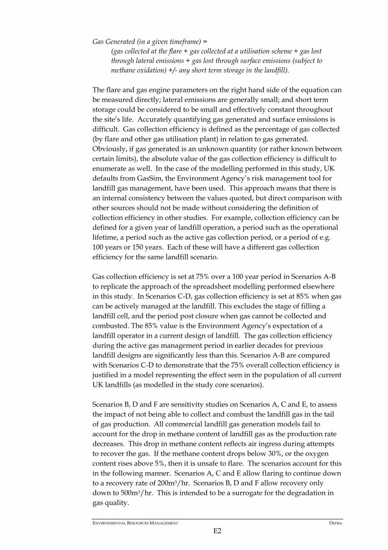
Gas Generated (in a given timeframe) =

(gas collected at the flare + gas collected at a utilisation scheme + gas lost through lateral emissions + gas lost through surface emissions (subject to methane oxidation) +/- any short term storage in the landfill).

The flare and gas engine parameters on the right hand side of the equation can be measured directly; lateral emissions are generally small; and short term storage could be considered to be small and effectively constant throughout the site’s life. Accurately quantifying gas generated and surface emissions is difficult. Gas collection efficiency is defined as the percentage of gas collected (by flare and other gas utilisation plant) in relation to gas generated. Obviously, if gas generated is an unknown quantity (or rather known between certain limits), the absolute value of the gas collection efficiency is difficult to enumerate as well. In the case of the modelling performed in this study, UK defaults from GasSim, the Environment Agency’s risk management tool for landfill gas management, have been used. This approach means that there is an internal consistency between the values quoted, but direct comparison with other sources should not be made without considering the definition of collection efficiency in other studies. For example, collection efficiency can be defined for a given year of landfill operation, a period such as the operational lifetime, a period such as the active gas collection period, or a period of e.g. 100 years or 150 years. Each of these will have a different gas collection efficiency for the same landfill scenario. Gas collection efficiency is set at 75% over a 100 year period in Scenarios A-B to replicate the approach of the spreadsheet modelling performed elsewhere in this study. In Scenarios C-D, gas collection efficiency is set at 85% when gas can be actively managed at the landfill. This excludes the stage of filling a landfill cell, and the period post closure when gas cannot be collected and combusted. The 85% value is the Environment Agency’s expectation of a landfill operator in a current design of landfill. The gas collection efficiency during the active gas management period in earlier decades for previous landfill designs are significantly less than this. Scenarios A-B are compared with Scenarios C-D to demonstrate that the 75% overall collection efficiency is justified in a model representing the effect seen in the population of all current UK landfills (as modelled in the study core scenarios). Scenarios B, D and F are sensitivity studies on Scenarios A, C and E, to assess the impact of not being able to collect and combust the landfill gas in the tail of gas production. All commercial landfill gas generation models fail to account for the drop in methane content of landfill gas as the production rate decreases. This drop in methane content reflects air ingress during attempts to recover the gas. If the methane content drops below 30%, or the oxygen content rises above 5%, then it is unsafe to flare. The scenarios account for this in the following manner. Scenarios A, C and E allow flaring to continue down to a recovery rate of 200m3/hr. Scenarios B, D and F allow recovery only down to 500m3/hr. This is intended to be a surrogate for the degradation in gas quality.


E3

Table E1.1 Scenario Model Definitions

Modelling Parameter Scenario A B C D E F Voidspace (Mt) 6 6 6 6 6 6 Area (Ha) 25 25 25 25 25 25 Depth (m) 24 24 24 24 24 24 No of Cells 12 12 12 12 12 12 Mass of waste in each cell (Mt) 0.5 0.5 0.5 0.5 0.5 0.5 Begin Filling

2005 2005 2005 2005 2005 2005

End Filling

2034 2034 2034 2034 2034 2034

Cap type

Clay Clay Clay Clay Clay Clay

Liner type

Composite Composite Composite Composite Composite Composite

Waste Composition See Table E1.2

See Table E1.2

See Table E1.2

See Table E1.2

See Table E1.2

See Table E1.2

Gas Collection Efficiency 75%

75%

85%

85%

85%

85%

Is the effect of no gas collection during the operational phase modelled?

No

No

Yes

Yes

Yes

Yes

Is the effect of inability to collect landfill gas from the tail of the curve (post utilisation) modelled?

Yes

No

Yes

No

Yes

No

Table E1.2 Waste Compositions Accepted at the Landfills

Waste Component Scenarios A-D 2006-2010

Scenarios A-D 2010-2015



Scenarios E-F (Diverted Inert Waste) 2005-2034

Newspapers 11.3 8.5 5.7 4.0 14.8 Magazines 4.8 3.7 2.4 1.7 6.3 Other paper 10.0 7.6 5.0 3.5 13.1 Liquid cartons 0.5 0.4 0.3 0.2 0.7 Card packaging 3.8 2.9 1.9 1.3 5.0 Other card 2.8 2.1 1.4 1.0 3.7 Textiles 2.3 1.8 1.2 0.8 3.0 Disposable nappies 4.3 3.3 2.2 1.5 5.6 Other miscellaneous 3.6 2.7 1.8 1.3 4.7 Garden waste 2.4 1.8 1.2 0.8 3.1 Other putrescible 18.3 13.8 9.2 6.4 24.0 <10mm Fines 7.1 5.3 3.6 2.5 9.3 Non-degradable

28.8 46.2 64.1 74.9 6.6

Total 100.0 100.1 100.0 99.9 100.0

Scenario A assumes that the landfill achieves the LFD diversion of biodegradable MSW targets. Gas collection efficiency is set at 75% overall and


E4

the waste is capped immediately after filling, to replicate the behaviour expected of the whole “landfill population” modelled in the rest of the study. Scenario B is the same as Scenario A, but in this instance the gas recovery in the tail of the gas generation curve is limited to 500m3/hr. Scenario C The landfill achieves the LFD diversion of biodegradable MSW targets. Gas collection efficiency is set at 85% overall, and the availability of gas for utilisation is determined by the degree of capping of the site, to replicate the actual capping procedures expected at a ‘normal’ landfill site. Scenario D is the same as Scenario C, but in this instance the gas recovery in the tail of the gas generation curve is limited to 500m3/hr. Scenario E. A landfill site is built as a gassing/large biodegradable landfill, which receives larger proportions of degradable waste than the landfills in Scenarios A and B. In this Scenario, the LATS targets are still achieved. More putrescible waste is diverted to the gas-producing landfill, where the landfill gas can be better controlled, and the bulk of the non-degradable fractions are diverted to recycling or the residue to inert landfills. In the GasSim model, non-degradable waste, which stands at 28% for a typical GasSim pre-2010 MSW waste stream (as in Scenarios A and B), is reduced to 6.6%, and the remaining 93.4% of waste is comprised of the same degradable fractions in a typical pre-2010 MSW waste stream scaled up in compositional terms. In this scenario, no compositional biodegradable MSW diversion targets are being followed for this particular landfill. Rather, these would have to be monitored across a portfolio of sites and waste treatment facilities. Scenario F is the same as Scenario E, but in this instance, the gas recovery in the tail of the gas generation curve is limited to 500m3/hr. All the landfills have the same morphology, capacity, and fill rate: 6 Mt of landfill void in a landfill of 25 ha area x 24 m deep, divided into 12 cells each of 20,833 m3 area and each cell accepting 0.5 Mt waste. Filling commenced in 2005 and is completed in 2034. The assessment period for greenhouse gas impacts is 150 years.

E1.2 RESULTS OF SCENARIO MODELLING

E1.2.1 Scenario A

Figure E1.1 shows the total bulk landfill gas (LFG) produced (top curve), total LFG utilisation by engines (middle curve) and total LFG flared (bottom curve). The landfill is able to support 0.5 MW of gas utilisation (utilising 300 m3/hr of LFG) almost from the start of filling, with a maximum generating capacity of 1.5 MW. The 1 MW gas engine (utilising 600 m3/hr of LFG) can be supported from 2010 until 2041 and the 0.5 MW gas engine until 2052. Figure E1.2 shows the total bulk LFG produced (top curve), surface emissions (middle curve) and


E5

lateral emissions bottom curve). The maximum surface emission is predicted to be 450 m3/hr in 2020. Cumulative global warming impacts for this scenario are 1.1 Mt CO2-eq.

Figure E1.1 Scenario A: LFG Generation, Utilisation and Flaring

Figure E1.2 Scenario A: LFG Generation, Surface and Lateral Emissions


E6

E1.2.2 Scenario B

Scenario B is the same as Scenario A, but with a reduced gas collection efficiency at the end of the landfill’s life. In this scenario, the 0.5MW gas engine does not run after 2035, and the flare only operates above 500m3/hr flowrate (Figure E1.3). In this scenario, cumulative global warming impacts of 1.39 Mt CO2-eq are predicted, compared with 1.11 Mt CO2-eq in Scenario A, an increase of 25% over the landfill’s gassing lifespan. This is ably shown in the surface emissions in Figure E1.4.

Figure E1.3 Scenario B: LFG Generation, Utilisation and Flaring


E7

Figure E1.4 Scenario B: LFG Generation, Surface and Lateral Emissions

E1.2.3 Scenario C

Figure E1.5 shows the total bulk LFG produced, total LFG utilisation by engines and total LFG flared. The landfill is also able to support 0.5 MW of gas utilisation almost from the start of filling, with a maximum generating capacity of 1.5 MW. The 1 MW gas engine can be supported from 2011 until 2041 (except for a gap year in 2023) and the 0.5 MW gas engine until 2054. It can be seen that both Scenario A and C are similar in LFG generation and gas utilisations, suggesting that the 75% average gas collection efficiency value used in modelling was a reasonable assumption to have made. Figure E1.6 shows the total bulk LFG produced, surface emissions and lateral emissions. The maximum surface emission is predicted to be 750 m3/hr in 2023. Cumulative global warming impacts of 1.23 Mt CO2-eq are predicted.


E8

Figure E1.5 Scenario C: LFG Generation, Utilisation and Flaring

Figure E1.6 Scenario C: LFG Generation, Surface and Lateral Emissions

E1.2.4 Scenario D

Scenario D is the same as Scenario C, but with a reduced gas collection efficiency at the end of the landfill’s life. In this scenario, the 0.5MW gas


E9

engine does not run after 2038, and the flare only operates above 500m3/hr flowrate (Figure E1.7). Cumulative global warming impacts of 1.54 Mt CO2-eq are predicted, compared with 1.23 Mt CO2-eq in Scenario C - an increase of 25% over the landfill’s gassing lifespan. This is shown in the surface emissions in Figure E1.8.

Figure E1.7 Scenario D: LFG Generation, Utilisation and Flaring

Figure E1.8 Scenario D: LFG Generation, Surface and Lateral Emissions


E10

E1.2.5 Scenario E

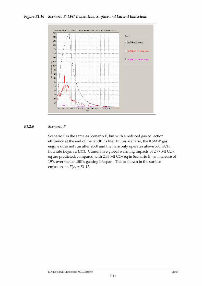
Figure E1.9 shows the total bulk LFG produced, total LFG utilisation by engines and total LFG flared and Figure E1.10 shows the total bulk LFG produced, surface emissions and lateral emissions from this scenario. It can be seen from Figure E1.9 that the site grows in gas utilisation capacity, being able to support 0.5 MW in 2008, 1.0 MW in 2011, 1.5 MW in 2014 and continuing to increase until 2032 when 4.5 MW installed capacity is achievable. After 2037, the site steadily loses capacity until 2073, when the last 0.5 MW gas engine is forecast to be decommissioned. The cumulative global warming impact from the site is higher than that from Scenarios A or C, at 2.33 Mt CO2-eq.

Figure E1.9 Scenario E: LFG Generation, Utilisation and Flaring


E11

Figure E1.10 Scenario E: LFG Generation, Surface and Lateral Emissions

E1.2.6 Scenario F

Scenario F is the same as Scenario E, but with a reduced gas collection efficiency at the end of the landfill’s life. In this scenario, the 0.5MW gas engine does not run after 2060 and the flare only operates above 500m3/hr flowrate (Figure E1.11). Cumulative global warming impacts of 2.77 Mt CO2-

eq are predicted, compared with 2.33 Mt CO2-eq in Scenario E - an increase of 19% over the landfill’s gassing lifespan. This is shown in the surface emissions in Figure E1.12.


E12

Figure E1.11 Scenario F: LFG Generation, Utilisation and Flaring

Figure E1.12 Scenario F: LFG Generation, Surface and Lateral Emissions


E13

E1.3 DISCUSSION AND CONCLUSIONS

One aim of this modelling exercise was to demonstrate that the approach used in modelling, assuming a 75% collection efficiency over 100 years, for the entire modelled landfill population, is realistic. Scenarios A and C were used to test this hypothesis. Scenario A represents the UK landfill population approach used to model the core study scenarios. Scenario C represents the behaviour of an individual landfill, where gas collection efficiency can be optimised, but operational areas restrict the gas collection efficiency during filling. These scenarios have very similar greenhouse gas impacts and power generation profiles (Table E1.3): • 1.11 and 1.23 Mt CO2-equivalents respectively emitted (7% variance

between the scenarios); and • 0.42 and 0.40 million MWh energy recovery potential respectively (5%

variance). The permitting regime expects 85% collection efficiency in the operational period of landfilling when active gas management is practicable. This means that during landfilling of individual cells, gas management may not be practicable. In the model example, a landfill with a modelled average of 75% gas collection efficiency, over a 100 year timeframe behaves similarly to a model of the same landfill site where the individual cells are represented and an 85% gas collection efficiency is expected where such gas can be collected by the gas collection infrastructure (but not during filling of the individual cells). On this basis, a 75% gas collection efficiency over 100 years would seem to be a reasonable assumption with regard to current landfill technologies and management. However, the results have been shown to be particularly sensitive to this assumption, and future estimates of climate change impacts associated with landfill would benefit from further work in this area. There are periods at the start and end of a landfill’s life during which gas collection is technologically impractical (at the end of a site’s life) or challenging (at the start of a site’s life). This modelling shows that a 100-year gas collection value of 75% could result in a lower lifetime (150 year) collection efficiency of approximately 59%. It should be realised that the nature of gas generation and emissions in the late stages of a landfill’s life are very site specific, and are not well understood. The modelling assumes first order decay but this is a simplification. Another aim of this modelling exercise was to examine whether the Landfill Directive BMW targets, aimed at reducing greenhouse gas emissions, might stifle the potential for energy recovery from landfill gas and increase net greenhouse gas emissions. Scenario E was devised to consider greenhouse gas estimates if residual waste is not landfilled in the same fashion as before, but instead the increasing inert fraction is diverted to inert waste landfills and the bioactive component is concentrated at a degradable waste landfill, where additional gas utilisation plant could be employed.


E14

Results show that when inert waste is diverted to inert waste landfills, and the degradable material is concentrated for gas utilisation, greenhouse gas emissions over the 150-year period are higher than those for landfills where diversion of BMW is an exact match with the Landfill Directive diversion targets. For example, Scenario E shows a greenhouse gas burden approximately 1.9 times than that of Scenario C (2.33 and 1.23 Mt CO2-eq respectively) (Table E1.3). However, these scenarios assume a different quantity of biodegradable waste throughput over the period assessed and so cannot be directly compared without normalising results. We did this by calculating emissions and energy generation potential per tonne of biodegradable waste sent to landfill in each scenario (1). Resulting estimates are shown in Table E1.4. These show scenario E to have both reduced greenhouse gas emissions and increased potential for energy generation, leading to further greenhouse gas savings. From this we can conclude that there is potential for greenhouse gas and energy benefits associated with concentrating degradable wastes in large biodegradable landfills, compared with reducing the biodegradable MSW content at all landfills at an equal rate. There are practical matters to be overcome, primarily relating to gas recovery on a landfill of this type, where there is a lower quantity of inert waste to act as the support medium for the degradable waste (2). However, the effect observed in Scenario E is by no means considered unachievable.

Table E1.3 Scenario Greenhouse Gas Emissions and Energy Generation Potential (Total over Period)

Scenario Greenhouse Gas Emissions (with gas management) (Mt CO2-eq)

Energy Generation Potential (Million MWh)

Greenhouse Gas Emissions (without gas management) (Mt CO2-eq)

Overall Lifetime Gas Collection Efficiency (%)

A 1.11 0.42 2.70 59 B 1.39 0.38 2.71 49 C 1.23 0.40 2.80 56 D 1.54 0.35 2.77 44 E 2.33 1.18 6.57 64 F 2.77 1.12 6.57 58

(1) Estimates as shown in Table E1.3, divided by the total biodegradable waste tonnage sent to landfills over the period assessed. (2) It is also generally acknowledged that inert wastes create pathways for gas transport within the landfill to gas recovery wells.


E15

Table E1.4 Scenario Greenhouse Gas Emissions and Energy Generation Potential – per Tonne of Biodegradable Waste Landfilled

Scenario Greenhouse Gas Emissions (with gas management) (tonnes CO2-eq)

Energy Generation Potential (MWh)

Greenhouse Gas Emissions (without gas management) (tonnes CO2-eq)

Overall Lifetime Gas Collection Efficiency (%)

A 0.47 0.18 1.14 59 B 0.59 0.16 1.15 49 C 0.52 0.17 1.19 56 D 0.65 0.15 1.17 44 E 0.42 0.21 1.17 64 F 0.49 0.20 1.17 58

A further aim of the modelling exercise was to ascertain the impact, in terms of gas collection efficiency, of not being able to manage the landfill gas in the tail of the gas production curve. The GasSim model used in this assessment does not automatically account for the dilution of methane content in old landfills. This occurs because the gas field is put under greater pressure to recover smaller amounts of generated gas, and atmospheric air can be drawn into the site when such suctions are applied. Scenarios A, C and E do not consider this effect, and allow GasSim to operate the abstraction flare down to 200 m3/hr. Scenarios B, D and F reflect A, C and E but, at the tail end of gas production, do not allow the flare to operate below 500 m3/hr. This is a surrogate value was designed to simulate the deterioration period for gas abstraction when the methane content and/or oxygen content is such that the gas can no longer be flared. Results show that for Scenarios B and D, the increase in greenhouse gas emissions is 25% above the corresponding scenarios A and C. For Scenario F, the increase is only 19%. There is a corresponding drop in electricity generation forecast for these scenarios also: between 8% for Scenario B and 5% for Scenarios D and F. The loss in power generation is only forecast at the tail of gas production, and this part of the forecast curve is also the most difficult to estimate. By modelling landfills without any gas management, we can compare greenhouse gas emissions and assess the overall lifetime gas collection efficiency of scenarios (shown in Table E1.3 to be between 44-64% for the six scenarios modelled). This range of lifetime gas collection efficiency values is much lower than is achievable during the operational period. While gas collection efficiency can be maintained on modern, engineered sites at 85% during the operational phases when gas collection is efficient, this does not hold when the uncontrollable tail of the gas generation curve is considered. As we have discussed above, collection efficiency can be different values for different timeframes of consideration. An estimated value for 150 year lifetime gas collection efficiency of between 56 – 64% is predicted if there are no losses of methane resulting from inabilities to collect gas at the tail end of

December 2006 - Defra, UKrandd.defra.gov.uk/Document.aspx?Document=WR0602_4748...Scenarios A-B are...

Documents

Transcript of December 2006 - Defra, UKrandd.defra.gov.uk/Document.aspx?Document=WR0602_4748...Scenarios A-B are...