RIETI Discussion Paper Series 03-E-007

Debt Deflation and Bank Recapitalization

Keiichiro Kobayashi

February 20, 2003

Abstract

In some recent financial crises, most of the domestic banks or the banking sector as a whole has become insolvent. We analyze the welfare effects of policy responses to bank insolvency by examining a modified version of the Diamond-Rajan model, in which we introduce fiat currency. The sources of inefficiency in our model are moral hazard in banking and the premature liquidation of bank assets. We assume that insolvency of the banking system is caused by an exogenous macroeconomic shock that destroys a portion of banks' assets.

If the government does not intervene in a very severe case of bank insolvency, a fire sale of all bank assets occurs, the economy becomes disintermediated, and price levels may fall (¥emph{debt deflation}).

We analyze the consequences of different policy responses to bank insolvency: (1) a deposit guarantee (without immediate recapitalization), (2) unlimited liquidity support, and (3) bank recapitalization through either cash creation (monetary policy) or bond issuance (fiscal policy). We show that bank recapitalization by fiscal measures isoptimal in our model. Our findings imply that Japan's protracted recession and deflation may have been caused by an inappropriate policy response to bank insolvency.

JEL Classification: E5, E6, G2, H3. Keywords: Financial crises, bank insolvency, debt deflation, recapitalization.

1

1 Introduction

In this paper, we analyze a banking crisis, subsequent debt deflation, and the policy

responses to the crisis in a model where fiat currency is introduced and contracts are

made in nominal terms.

In the recent theoretical research on banking crises, many theories have been proposed

concerning the mechanism by which financial crises occur (Diamond and Dybvig [1983],

Postlewaite and Vives [1987], and Allen and Gale [1998, 2000, 2001]). But there are

not so many theories that explain the difference of recovery paths from the crises in

accordance with different policy responses. For example, Diamond and Dybvig (1983),

Freixas, Parigi, and Rochet (1999), and Martin (2001) discuss the policies to prevent bank

runs, but not policy responses to bank insolvency. Only a few authors like Diamond and

Rajan (2002a, b), Bergoeing, et al. (2002), and Boyd, Chang, and Smith (2000) consider

ex post policy responses to financial crises.

The world has experienced a large number of banking crises in the last three decades.

Caprio and Klingebiel (1999) identified 113 systemic banking crises that had occurred

in 93 countries since the late 1970s, along with 50 borderline and smaller banking crises

in 44 countries over the same period. In analyzing these experiences, researchers have

come to pay more attention to bank insolvency than to bank runs. Recent crisis episodes

suggest that bank insolvency is the central problem to be rectified and that a temporary

shortage of liquidity is basically a symptom. Diamond and Rajan (2002a) also refer

to the theoretical possibility of two-way linkage between bank insolvency and liquidity

shortages.

One common observation concerning financial crises is the decline of the inflation rate

after the onset of a banking crisis (Boyd et al. [2001]). The United States experienced

severe deflation associated with a rash of bank failures in the 1930s, and Japan is now

experiencing a bout of deflation following the onset of a banking crisis in the late 1990s.

Boyd et al. (2001) show that the onset of a banking crisis decreases the growth rate of

M2, which is a significant element contributing to inflation. The low inflation or deflation

associated with a banking crisis may be modeled as debt deflation (Fisher [1933]). In

2

this paper we formalize the notion of debt deflation in a simple model.

Several facts about the recovery paths from banking crises have been found by case

studies and empirical research on recent financial crises (see, for example, Claessens,

Klingebiel, and Laeven [2001], Alexander et al. [1997], Caprio and Klingebiel [1996]).

Honohan and Klingebiel (2000) find that open-ended liquidity support, regulatory for-

bearance, and an unlimited deposit guarantee are all significant contributors to the fiscal

cost of resolving a banking crisis. They also find that liquidity support significantly

increases the output loss or delays the economic recovery. (This result is confirmed by

Bordo et al. [2001], who used a broader data set.) Boyd et al. (2001) also claim that

incremental expenditures for banking system bailouts may increase output losses. On

the other hand, Claessens, Klingebiel, and Laeven (2001) show that liquidity support

and a deposit guarantee may be effective in promoting a recovery of profitability in the

corporate sector if these measures are combined with the establishment of an asset man-

agement agency. Although empirical analyses have not produced a consensus concerning

the effects of bank bailouts, it seems the case that a temporizing policy such as liquid-

ity support or a deposit guarantee without the restoration of bank solvency may hinder

economic recovery and magnify the fiscal cost.

In any case the banking system must be recapitalized in order for an economic system

hit by a banking crisis to restore its normal functions. There are many important practi-

cal issues concerning bank recapitalization, such as the source of funds, the loss sharing

by depositors, the incentive mechanism for banks’ management, the design of financial

instruments, and the exit strategy for the government (Honohan [2001]). Whether or

not to monetize the cost of recapitalization is one big issue in the policy debate. For

example, inflation targeting, or extraordinary monetary easing, has become the focus of

the macroeconomic policy debate in Japan since the financial crisis of 1998. One of the

objectives of inflation targeting in today’s Japan would obviously be to monetize the

cost of recapitalizing the banking system. Thus, the provision of a theoretical basis for

judging the costs and effects of a monetization policy is very important as a practical

matter for crisis-affected countries. The recent crisis episodes show that bank bailout

3

costs are typically not monetized (Boyd et al. [2001]). We can ask whether there was

any economic ground for the policymakers’ decision not to monetize the cost of bank

recapitalization in those episodes.

Our aim in this paper is to formalize debt deflation, i.e., the decline of the infla-

tion rate associated with a banking crisis, and to analyze the effects of different policy

responses to bank insolvency. In order to model the debt deflation, we construct a vari-

ant of the Diamond-Rajan model (Diamond and Rajan [2001]) in which we introduce

fiat currency using a cash-in-advance constraint. In this variant Diamond-Rajan model,

banks are subject to moral hazard, i.e., inefficient use of capital, but this can be deterred

by the threat of bank runs by depositors - a threat that is made credible by the use of

demand deposit contracts. On the other hand, if bank runs occur, banks are forced to

liquidate their assets prematurely. Thus, in this model the sources of inefficiency are

moral hazard and the premature liquidation of bank assets.

In our model, we do not describe how financial crises occur; we merely posit that

all banks become insolvent as a result of an unspecified macroeconomic shock (e.g., the

bursting of an asset-price bubble or a fall in the currency exchange rate) that suddenly

decreases the value of all bank assets. Taking this banking system insolvency as given,

we focus our analysis on the welfare properties of the following policy responses: (1)

a deposit guarantee, (2) unlimited liquidity support, (3) bank recapitalization through

cash creation (monetary recapitalization), and (4) bank recapitalization through bond

issuance (fiscal recapitalization).

If the government takes no action in response to bank insolvency, all households will

withdraw their deposits immediately, since they know that the banks’ assets are less than

their liabilities. In this case, all the banks experience depositor runs, all their assets must

be liquidated prematurely, price levels fall, and the welfare of households deteriorates.

If the government implements a deposit guarantee policy and/or an unlimited liq-

uidity support policy, it is easily shown that, while bank runs are prevented, banks are

inevitably subject to moral hazard. This is because under these policies the government

gives the banks a commitment to provide them resources without limit.

4

In order to avoid generating moral hazard, the government must combine the provi-

sion of additional resources ex ante to banks (recapitalization) with a credible declaration

that it will not provide any more ex post. The government has two options in financing

the cost of recapitalization: monetization or taxation. In the case where the government

implements the bank recapitalization by creating cash (monetary recapitalization), it is

shown that moral hazard cannot be prevented, since the monetary recapitalization af-

fects the banks’ incentive to hold cash reserves through the cash-in-advance constraint.

In the case where the government implements the bank recapitalization by issuing bonds

(fiscal recapitalization), it is shown that the optimal outcome is achieved, avoiding both

moral hazard and the premature liquidation of assets.

The rest of the paper is organized as follows: Section 2 describes the basic model.

Section 3 analyzes debt deflation, which is triggered by bank insolvency resulting from

an unexpected macroeconomic shock. Section 4 compares the welfare effects of several

policy options. And Section 5 presents the conclusion.

2 Basic Model

The economy consists of continua of consumers and of banks. For simplicity of exposition,

we shall normalize the measure of each continuum to 1. But we assume that each bank

has infinitely many consumers as its depositors.1 There is also the government. The

economy continues for two consecutive periods bounded by three dates: t = 0, 1, 2.

There is one type of good (consumer good) in this economy that can be consumed by

consumers. Banks can transform the consumer good into productive capital, and only

banks can use capital and produce the consumer goods at date 1 and date 2.

2.1 Consumers

A consumer maximizes his utility u(c0)+βu(c1)+β2u(c2), where u(c) satisfies the usual

neoclassical properties (u0(c) > 0, u00(c) < 0, limc→0 u0(c) = ∞), ct is the consumption1This statement can be justified by assuming that a bank is indexed by α where α ∈ [0, 1], while a

consumer is indexed by (α, γ) where (α, γ) ∈ [0, 1]2.

5

at date t and β is the time discount factor. For simplicity we assume u(c) = ln c in

what follows. At date 0 each consumer is endowed with E units of consumer goods and

M units of useless paper that is provided by the government and is called “cash.” The

government levies a tax of M units of cash on each consumer at date 2. Although cash

is intrinsically useless for consumers, we posit the following cash-in-advance constraint

that makes cash a medium of exchange:

Assumption 1 (Cash-In-Advance Constraint) A consumer must use cash to purchase

the consumer good.

There is no endowment for consumers at dates 1 and 2. There are three assets available

to consumers as stores of value: the consumer good (stored rather than consumed), cash,

and bank deposits.2 If a consumer stores y units of the consumer good at date t, then he

will still have y units of the goods at date t+1. This is storage technology. Alternatively,

a consumer can deposit the consumer goods and/or cash that he has at date t in a bank

in exchange for a nominal claim on the bank (i.e., a demand deposit) Dt at date t. We

make the following assumption for the deposit contract:

Assumption 2 The deposit contract can be made only in nominal terms. A contract in

real terms between consumers and banks is not allowed.

This assumption can be justified as follows: Though it may be possible to observe a

change of price levels, it is not easy for depositors or banks to verify the amplitude of

the change; therefore, real-term contracts cannot readily be implemented in the private

sector. For simplicity we prohibit real-term contracts in our model. We will see in

Section 2.2 that the following characteristic of the demand deposit contract is necessary

to prevent moral hazard for banks.

Assumption 3 A demand deposit is a contract between a bank and a consumer such

that the consumer (depositor) can withdraw any amount of cash up to his bank balance

at any time.2In the equilibrium where the nominal interest rate is positive, consumers do not hold cash, but they

hold bank deposits.

6

This assumption states that consumers can withdraw any amount of cash just before

they buy the consumer good, implying that the cash-in-advance constraint does not

enter in the consumer’s optimization program as it usually does in ordinary cash-in-

advance models (see, for example, Sargent [1987]). As we will state in Section 2.2 that

banks’ production technology is more efficient than storage technology, we consider for

a moment the consumer’s optimization problem on the premise that consumers choose

bank deposits as their only assets.3 In this case, consumers solve the following problem

taking prices (p0, p1, p2), nominal interest rates (i0, i1), endowments (E,M), and the tax

T2 =M as given.

(PC) maxc0,c1,c2

u(c0) + βu(c1) + β2u(c2)

subject to p0c0 +D0 ≤ p0E +M,p1c1 +D1 ≤ (1 + i0)D0,p2c2 + T2 ≤ (1 + i1)D1,

(1)

where u(ct) = ln ct, and Dt is the demand deposit remaining at date t.

2.2 Banks

Our model of the banking sector is a simplified version of the Diamond-Rajan model

(Diamond and Rajan [2001]).

Production Technology At date 0 a bank can transform K0 units of the consumer

good that are deposited by consumers into the same amount of capital, i.e., K0 units

of capital. Only banks, not consumers, can use the capital to produce the consumer

good. Suppose that a bank (bank α, 0 ≤ α ≤ 1) forms capital of K0α at date 0. Bank αcan produce AK0α units of the consumer good at date 1, while the capital depreciates

3Grossman and Weiss (1983) also construct a model in which they impose a restriction that only

banks hold cash and the depositors do not, while in our model the banks’ decisions on holding cash

reserves are endogenous, as discussed in Section 2.4.

7

completely to zero.4 If bank α sells y1α units of the consumer good to consumers, it can

invest the rest and form capital of K1α, where K1α = AK0α− y1α. At date 2 bank α canproduce AK1α units of the consumer good, while its capital K1α depreciates completely

to zero. This is the standard AK-technology of the neoclassical growth model. We

assume

1 < A,

which implies that the bank’s production technology is more efficient than storage tech-

nology. We assume that bank α can also use its capital inefficiently. For simplicity of

analysis, we assume the following:

Assumption 4 Bank α can attain either high productivity (A) by efficient use of capital

K0α or low productivity (a) by inefficient use of capital, where

1 ≤ a < A. (2)

Bank α’s choice variables are (1) the efficiency in use of capital (efficient or inefficient),

and (2) the amounts of sale and investment (see the bank’s problem (PB) below). Bank

α obtains private utility at dates 1 and 2 if it continues to operate. The private utility at

date t (Ut) is 0 if bank α stops its operation at date t, b if it chooses inefficient use of

capital, and b−² if it chooses efficient use of capital, where ² (0 < ² < b) is the effort thatis necessary to use capital efficiently. The effort ² is observable but not verifiable for the

other agents so that contracts contingent on ² is infeasible. A bank’s primary objective

is to maximize the present value of its private utility

V ≡ βU1 + β2U2.

Like Diamond and Rajan, we assume the following “relation-specificity” in this produc-

tion technology of banks: Only bank α can use K0α most efficiently, since bank α has

relation-specific knowledge that other banks do not have about K0α, such as the detailed

structure of the business model and the efficient use of the equipment in question. If

4We assume for simplicity that the capital investment by a bank is reversible: the bank can transform

the capital back into the consumer good at any time before the production takes place.

8

bank α0 (α0 6= α, 0 ≤ α0 ≤ 1) takes over K0α, it can produce a0K0α units of the consumergood at date 1, while the capital K0α depreciates to zero. We assume

1 ≤ a0 < a < A. (3)

After selling y0 units of the consumer good, bank α0 can form K 01 = a

0K0α − y0, and canproduce AK 0

1 units of the consumer good at date 2, while K01 depreciates to zero.

Bank’s Problem Competition for depositors among banks forces a bank to maximize

their value, since otherwise it cannot collect deposits and is forced to stop operating,

and its private utility is driven down to zero. When the nominal interest rate is strictly

positive (it > 0), the competition among banks also makes them commit to efficient use

of capital, and they obtain U1 = U2 = b− ²; a bank chooses efficient use of capital if theother banks use capital efficiently, since otherwise it cannot collect deposit and is forced

to stop operating. (See Lemma 1 for the case where it = 0.) Thus a bank (bank α)

solves the following problem taking prices (p0, p1, p2), interest rates (i0, i1) where i0 > 0

and i1 > 0, and initially deposited consumer goods (E) as given.

(PB) maxy0,y1,y2

p0y0 +p1

1 + i0y1 +

p2(1 + i0)(1 + i1)

y2

subject to

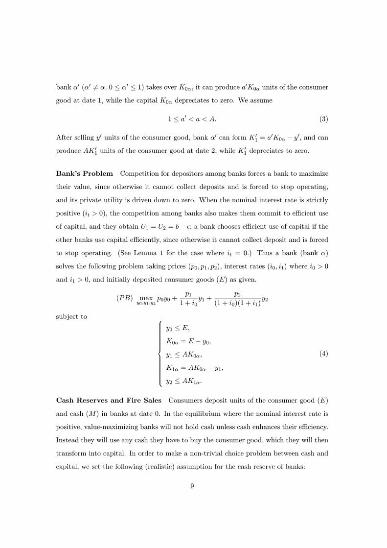
y0 ≤ E,K0α = E − y0,y1 ≤ AK0α,K1α = AK0α − y1,y2 ≤ AK1α.

(4)

Cash Reserves and Fire Sales Consumers deposit units of the consumer good (E)

and cash (M) in banks at date 0. In the equilibrium where the nominal interest rate is

positive, value-maximizing banks will not hold cash unless cash enhances their efficiency.

Instead they will use any cash they have to buy the consumer good, which they will then

transform into capital. In order to make a non-trivial choice problem between cash and

capital, we set the following (realistic) assumption for the cash reserve of banks:

9

Assumption 5 Let Wt be the withdrawal demand from a bank’s depositors at date t.

The bank can pay Wt in two ways. (1) It can use a cash reserve Mt−1 that was set at

date t− 1. (2) It can sell the consumer good yt at date t and use the cash income ptyt torepay the depositors at date t. We will call the second method a “fire sale.” If the bank

uses the fire sale, it incurs a “deadweight loss”: 1−xx yt units of the consumer goods where

0 < x < β.

The deadweight loss 1−xx yt is not incurred if the proceeds of a sale are kept as a cash

reserve for date t+ 1.

This assumption states that a bank facing withdrawals by depositors must raise cash

through an inefficient fire sale of goods if it does not have a sufficient cash reserve. The

assumption implies that a bank must produce 1xyt > β−1yt in order to sell yt in the fire

sale. This loss represents the inefficiency involved in a fire sale of bank assets in reality.

Note that the deadweight loss is not incurred if the proceeds of the sale are not paid out

at the same date but are kept as a cash reserve for the next date. This feature of the

deadweight loss can be justified as follows: The inefficiency of a fire sale occurs when a

bank sells an asset to someone who cannot use it most efficiently. A bank cannot find

the best buyer if it does not have enough time to search among the possible buyers. And

banks that do not have enough reserves on hand must raise cash immediately to pay

their depositors; they have no time to search for good buyers; they suffer the deadweight

loss by selling the goods to suboptimal buyers. On the other hand, banks that have

enough reserves have enough time to find the best buyer since they do not need to pay

out the proceeds of the sale immediately; they do not incur the deadweight loss. This is

the reason why a deadweight loss is incurred in our model only when the bank pays out

the proceeds of the sale to the depositors on the same date.

Demand Deposit The above relation-specific technology justifies the aforesaid char-

acteristic of demand deposits (Assumption 3). Suppose that D0 is the demand deposit

remaining at the end of date 0. As we will see later, in the equilibrium the date-0 with-

drawal p0c0 is equal to M , y0 = c0, and no fire sale occurs at date 0. In this case, if the

10

contract made at date 0 between the consumer and bank α is not renegotiated at a later

date, then the value of the deposit must be D0 =p11+i0

y1 +p2

(1+i0)(1+i1)y2 +M , where

(y1, y2) is the solution to (PB). But the relation-specific technology prevents banks from

committing not to renegotiate after a contract is established. We assume the following:

Assumption 6 Bank α can walk away at any time, leaving the capital (K0α between

date 0 and date 1, or K1α = AK0α − y0 between date 1 and date 2) for the depositors.If bank α walks away, the only thing the depositors can do is to deposit the capital that

bank α left in another bank α0 and let bank α0 use the capital.

After forming the relation-specific capital K0α, bank α, knowing that it can walk away

at any time, has an incentive to offer D00 = maxy01,y02p11+i0

y01 +p2

(1+i0)(1+i1)y02 +M , where

y01 ≤ aK0α and y02 ≤ a(aK0α − y01), instead of D0 to the consumer. Assumption 6 andequation (3) imply that the rational consumer will always accept the offer D00.

Therefore, if the contract between consumers and banks is a renegotiable debt con-

tract, banks will always renegotiate their obligation down to D00, they will choose ineffi-

cient use of capital, and productivity will decline to a. Diamond and Rajan (2001) point

out that demand deposits are a tool for banks to credibly commit not to renegotiate later.

The intuition is as follows. Suppose that the demand deposit contract gives depositors

the right to withdraw the full amount of their deposit from bank α at any time. If bank

α tries to renegotiate at a time between date 0 and date 1, depositors will rationally

exert their right to withdraw, and this will result in a run on the bank. The bank run

results in the fire sale of all the bank’s assets, and bank α is forced to stop operating

at date 1. In this case, bank α cannot obtain the private utility Ut at dates 1 and 2.

Anticipating this result, a bank will not try to renegotiate as long as the date 0 contract

between depositors and banks is a demand deposit. The same argument implies that

banks will not renegotiate at any time between dates 1 and 2. In Section 2.4 we will

show more rigorously that demand deposits prevent renegotiation in the equilibrium.

In our model, depositors withdraw cash, not the consumer good as in the Diamond-

Rajan model. This difference necessitates the following assumption for demand deposits

to prevent renegotiation.

11

Assumption 7 A consumer who withdraws his deposit from a bank can deposit the cash

he has withdrawn in another bank at the same rate of return (i0, i1).

This assumption states that banks must accept deposits from consumers at any time on

the same terms and conditions. Unless Assumption 7 holds, consumers who withdraw

their deposits in a run on a bank must either hold the proceeds as cash or buy consumer

goods and store them. Since holding cash or storing consumer goods provides less con-

sumption to consumers, they may rationally accept the renegotiation by banks instead

of withdrawing their deposits in bank runs. Therefore, both Assumptions 3 and 7 must

hold for demand deposits to prevent renegotiation in our model, while Assumption 3 is

sufficient in the Diamond-Rajan model, where the deposit contract is made in real terms.

2.3 Timing of Events

We summarize the timing of events in our model. At date 0, the consumers are endowed

with E units of the consumer good and M units of cash. They deposit E and M in

banks in exchange for the nominal claims D (demand deposits) on the banks. After

receiving E and M , banks have a chance to buy and sell the consumer goods at price

p0 among themselves to adjust their asset portfolio and cash reserves. (In the Financial

Intermediation Equilibrium [FIE] defined in Section 2.4 no trading occurs.) Then con-

sumers withdraw p0c0 units of cash from banks and buy c0 units of the consumer good.

It is shown in Section 2.4 that the withdrawal p0c0 must be equal to the cash reserve M

in the FIE. The remaining demand deposits become D0 = D − p0c0. At this stage, abank has E − c0 units of the consumer good and M units of cash as its assets and D0

as its liabilities. Then banks have another chance to buy and sell the consumer good at

price p0 among themselves in order to achieve their optimal level of cash reserves M0.

(M0 =M in the FIE.) The banks next transform the consumer good E − c0 into capitalK0 = E − c0. After forming their capital, banks have an incentive to renegotiate withthe depositors, but they do not actually offer renegotiation in the equilibrium, since such

an offer would induce a run on the bank that made it.

At date 1, the banks produce AK0 units of the consumer good. The demand deposit

12

becomes (1 + i0)D0. Consumers withdraw p1c1 units of cash and buy c1 units of the

consumer good. If the withdrawal p1c1 > M0, a fire sale occurs. In the equilibrium

p1c1 =M0 =M . The remaining demand deposits become D1 = (1+ i0)D0− p1c1. Thenbanks have a chance to sell and buy the consumer good at price p1 among themselves

so as to achieve their desired level of cash reserves M1. (No trade occurs, and M1 = M

in the FIE.) Then banks transform the remaining consumer goods AK0− c1 into capitalK1 = AK0 − c1. After forming this new capital, banks again have an incentive to

renegotiate, but again they do not actually offer renegotiation in the equilibrium.

At date 2, the banks produce AK1 units of the consumer good. The demand deposits

become (1 + i1)D1. Consumers withdraw p2c2 units of cash and buy c2 units of the

consumer good. If p2c2 > M1, a fire sale occurs. In the equilibrium p2c2 = M1 = M .

The remaining demand deposits become D2 = (1 + i1)D1 − p2c2. The government thenrequires consumers to pay a tax T2 =M . Consumers withdraw T2 from banks, they pay

the tax, and the economy ends. In the FIE, D2 = T2 =M must hold.

2.4 Optimal Equilibrium

We define the Financial Intermediation Equilibrium (FIE) as follows:

Definition 1 The Financial Intermediation Equilibrium is the set of prices (p0, p1, p2, i0, i1),

endowments (E,M), tax (T2), and allocation (c0, c1, c2) such that (1) the allocation

(c0, c1, c2) is the solution to (PC) given the prices, endowments, and tax; (2) (y0, y1, y2)

= (c0, c1, c2) is the solution to (PB) given the prices and the endowment E; (3) Given

the prices and the withdrawals (p0c0, p1c1, p2c2), banks rationally choose to hold cash re-

serves of Mt = pt+1ct+1 at each date t = 0, 1; (4) The money market clears Mt = M

at each date t; (5) Given the prices, banks rationally withhold offering renegotiation to

depositors.

We will show that the optimal allocation is attainable in the Financial Intermediation

Equilibrium. The optimal allocation is given by the following social planner’s problem:

(PO) maxc0,c1,c2

u(c0) + βu(c1) + β2u(c2)

13

subject to c0 ≤ E,c1 ≤ A(E − c0),c2 ≤ A2(E − c0)−Ac1.

(5)

The solution (c∗0, c∗1, c∗2) is uniquely determined by the resource constraints and the first-

order conditions (FOCs):u0(c∗0)βu0(c∗1)

=u0(c∗1)βu0(c∗2)

= A. (6)

Since we assume u(ct) = ln ct, the solution is

c∗0 =E

1 + β + β2, c∗1 = βAc∗0, c

∗2 = β2A2c∗0. (7)

We assume that the parameters satisfy the following:

Assumption 8 The parameters β and x satisfy (2−x)β2+(1−x)β > 1 and (2−x)β > 1.

For example, β ≥ .9 and x ≤ .8 satisfy this condition. This assumption guarantees thatAssumptions 3 and 7 are sufficient to prevent renegotiation in the FIE. In a decentralized

economy, the consumer’s problem is (PC), the solution to which is characterized by the

following FOCs:u0(c∗0)βu0(c∗1)

=p0p1(1 + i0),

u0(c∗1)βu0(c∗2)

=p1p2(1 + i1). (8)

The bank’s problem is (PB), the solution to which is characterized by

p0p1(1 + i0) =

p1p2(1 + i1) = A. (9)

It is easily shown that the set of the prices (p∗0, p∗1, p∗2, i∗0, i∗1) ≡ (Mc∗0, Mc∗1, Mc∗2, β−1 −

1,β−1 − 1) and the allocation (c∗0, c∗1, c∗2) satisfies the FOCs (8) and (9). We can nowdemonstrate the following proposition:

Proposition 1 The set of the prices (p∗0, p∗1, p∗2, i∗0, i∗1) and the allocation (c∗0, c∗1, c∗2) is the

Financial Intermediation Equilibrium.

(Proof) It is sufficient to show that banks rationally set the cash reserve at Mt =M for t = 0, 1,

and that they rationally withhold offering renegotiation. Given the prices, the withdrawals at

14

each date are p∗0c∗0 = p∗1c

∗1 = p∗2c

∗2 = M . At the beginning of date 0, each bank has M units

of cash, as the consumers deposit all their cash. Before depositors withdraw p∗0c∗0, banks can

change the level of their cash reserve (R) by buying and selling the consumer goods at price p∗0.

If R < p∗0c∗0 = M , banks incur a deadweight loss (Assumption 5). Thus banks desire for R to

be greater than or equal to M . Since banks have another chance to sell and buy the consumer

goods at the same price p∗0 after the withdrawal of p∗0c∗0, they are indifferent whether R = M or

R > M . Therefore, banks set their reserves at the level of the money supply M .

When depositors withdraw p∗0c∗0, the cash M is withdrawn temporarily but is returned to the

banks on the same date in the form of the proceeds from sales of the consumer good y0 = c∗0.

At this point banks, anticipating that withdrawals at date 1 will be p∗1c∗1 = M , have the chance

to change the level of their cash reserves (M0) by buying and selling the consumer good at p∗0

among themselves. If a bank setsM0 to be greater than the expected withdrawals (M), it loses the

opportunity to produce the consumer good, incurring the opportunity cost: {A p∗1p∗0−1}(M0−M) =

(β−1− 1)(M0−M) units of cash. Thus M0 must be no greater than M . If a bank sets M0 < M ,

it can buy 1p∗0(M −M0) units of the consumer good and produce

Ap∗0(M −M0) at date 1. But at

date 1 the bank must sell part of its output in a fire sale in order to obtain cash M −M0 to pay

out M to the depositors. The payoff is Ap∗1p∗0(M −M0) − 1

x(M −M0) = (β−1 − x−1)(M −M0),

which is less than zero because of Assumption 5. Therefore banks set M0 = M given the prices

(p∗0, p∗1). It is shown that M1 =M by the same argument.

Next we show that banks rationally withhold renegotiation. In this equilibrium the budget

constraint of (PC) implies that (1 + i∗1)D1 = p∗2c∗2 + T2 = 2M , (1 + i∗0)D0 = p∗1c∗1 + 2βM =

(1 + 2β)M , and D0 = (1 + 2β)βM . Therefore the bank’s liability at the end of date 0 is

D0 = (1 + 2β)βM , while the bank’s assets are M units of cash and E − c∗0 units of capital.The bank has the incentive to renegotiate with depositors at a time after it forms the capital

K0 = E − c∗0 and before it produces the date 1 consumer good AK0. If at this time the bank

offers renegotiation and experiences a run by the depositors, then it will be forced to transform

E − c∗0 back into units of the consumer good and to sell them in a fire sale. In this case the

total cash the bank can pay out becomes M + p∗0x(E − c∗0) = (1 + βx + β2x)M . Assumption 8

guarantees that the bank will go bankrupt if there is a run on it by depositors at the end of date

0. Anticipating this result, banks rationally withhold renegotiation at the end of date 0.

Similarly, at the end of date 1 when the bank has the incentive to renegotiate, its liability

is D1 = 2βM , while the total cash the bank can pay out after the fire sale is (1 + βx)M . Thus

Assumption 8 guarantees that the bank will go bankrupt if a bank run occurs, and that banks

15

rationally withhold renegotiation at the end of date 1. (End of Proof)

Thus in the FIE, the most efficient use of capital and the optimal consumption

allocation are realized by demand deposit contracts between banks and consumers.

3 Banking Crisis

The recent episodes of banking crises have often involved the emergence and subsequent

collapse of an asset-price bubble. In this paper we do not analyze how the bubble emerges

or how it collapses. Our focus is on how the collapse affects the banking sector and on the

overall economy. Thus in our model we describe the bubble’s collapse as an unexpected

macroeconomic shock that destroys a portion of the real output of the economy. The

occurrence of this shock is assumed to be a measure-zero event, in the sense that the

agents in the economy have no expectation of the shock beforehand. We can modify

our model to treat the macro shock as a random variable the probability distribution of

which is known ex ante to the agents. But this modification does not essentially change

the results that we describe below, since our results mainly concern the responses of

the economic agents after the shock hits. Thus for simplicity of exposition we assume

that the ex ante probability of the shock (bubble collapse) equals zero5, and that all

consumers and banks at date 0 make their contracts on the premise that prices will

become (p∗0, p∗1, p∗2, i∗0, i∗1).

3.1 Bubble Collapse, Price Adjustment, and Zero Nominal Interest

Rate

We formalize the bubble collapse at the beginning of date 1 as follows. At a time after

AK0 = A(E− c∗0) units of the consumer good are produced and the equilibrium price p∗1

is announced but before the goods are sold to consumers, a macro shock λ (0 ≤ λ < 1)

hits the economy unexpectedly and destroys (1 − λ)AK0 of each bank’s output. Since

5This modeling strategy is same as Loewy (1991). Burnside, Eichenbaum, and Rebelo (2001) also

adopt the same modeling strategy to analyze currency crises.

16

the ex post output is λAK0 after the bubble collapse at date 1, the optimal allocation

after the shock becomes (c1, c2) = (λc∗1,λc∗2). The optimal allocation is realized as an

equilibrium outcome by the new price system (p1, p2, i1) = (λ−1p∗1,λ−1p∗2, i∗1). We will

show that the optimal equilibrium is realized by a standard price adjustment process if

depositors cannot make a run on banks before the price system changes.

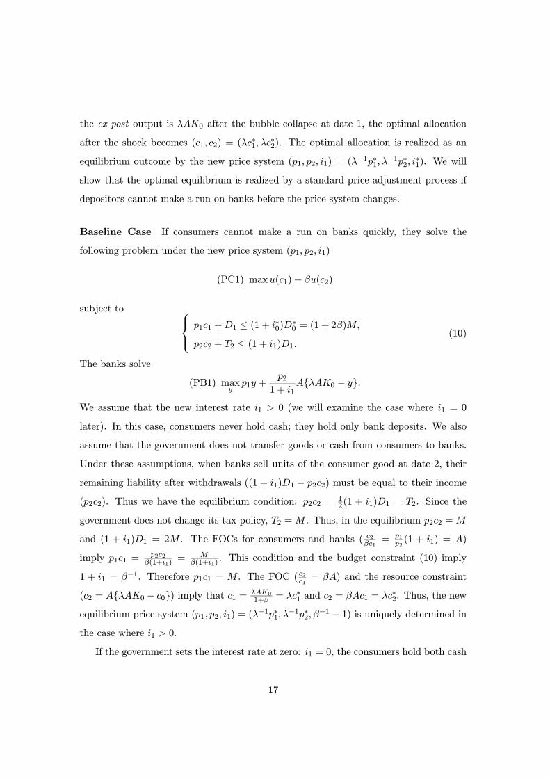
Baseline Case If consumers cannot make a run on banks quickly, they solve the

following problem under the new price system (p1, p2, i1)

(PC1) maxu(c1) + βu(c2)

subject to p1c1 +D1 ≤ (1 + i∗0)D∗0 = (1 + 2β)M,p2c2 + T2 ≤ (1 + i1)D1.

(10)

The banks solve

(PB1) maxyp1y +

p21 + i1

A{λAK0 − y}.

We assume that the new interest rate i1 > 0 (we will examine the case where i1 = 0

later). In this case, consumers never hold cash; they hold only bank deposits. We also

assume that the government does not transfer goods or cash from consumers to banks.

Under these assumptions, when banks sell units of the consumer good at date 2, their

remaining liability after withdrawals ((1 + i1)D1 − p2c2) must be equal to their income(p2c2). Thus we have the equilibrium condition: p2c2 =

12(1 + i1)D1 = T2. Since the

government does not change its tax policy, T2 =M . Thus, in the equilibrium p2c2 =M

and (1 + i1)D1 = 2M . The FOCs for consumers and banks ( c2βc1 =p1p2(1 + i1) = A)

imply p1c1 =p2c2

β(1+i1)= M

β(1+i1). This condition and the budget constraint (10) imply

1 + i1 = β−1. Therefore p1c1 = M . The FOC ( c2c1 = βA) and the resource constraint

(c2 = A{λAK0 − c0}) imply that c1 = λAK01+β = λc∗1 and c2 = βAc1 = λc∗2. Thus, the new

equilibrium price system (p1, p2, i1) = (λ−1p∗1,λ−1p∗2, β−1 − 1) is uniquely determined in

the case where i1 > 0.

If the government sets the interest rate at zero: i1 = 0, the consumers hold both cash

17

and bank deposits. We can show that banks will choose the inefficient use of capital if

the nominal interest rate is zero:

Lemma 1 Suppose that the economy is in an equilibrium where the nominal interest rate

is zero and banks continue to operate at dates 1 and 2. Each bank chooses the inefficient

use of capital and the aggregate productivity of the economy becomes a.

(Proof) Since the banks continue to operate at dates 1 and 2 under a zero nominal interest rate,

the prices satisfy the FOC for the banks:

p1p2= A, (11)

where A is the productivity of capital, which is A if the bank chooses the efficient use of capital,

and is a if it chooses the inefficient use. We will prove that a bank holds only cash rather than

capital if the other banks choose efficient use of capital. Suppose that all banks choose the

efficient use of capital. Then p1p2= A. This condition and Assumption 4 imply that a bank can

obtain the same return A by holding cash without exerting effort ². Therefore when a bank enters

into deposit contracts with depositors at date 1, it promises them the same return as the other

banks, and it holds only cash, because by doing so the bank can fulfill the promise made to the

depositors and can save the effort ² that must be exerted to fulfill the promise by using capital.

Therefore no banks will hold capital in the equilibrium where i1 = 0 and p1p2= A. This is a

contradiction, since if no banks hold capital then p1p2= A does not hold. Thus, in the equilibrium

where i1 = 0 it must be the case thatp1p2= a, and all banks choose the inefficient use of capital.

(End of Proof)

This lemma says that if i1 = 0 the banks never promise the efficient use of capital in

the first place. Therefore the demand deposit contract, which does not allow subsequent

renegotiation, cannot prevent the inefficiency of moral hazard when i1 = 0. The impli-

cation of this lemma is similar to Smith’s view that the Friedman rule is not the optimal

policy in the economy where the financial intermediaries play a significant role (Smith

[2002]).

It is easily shown that if i1 = 0 and the depositors cannot make runs on banks,

there exists a continuum of equilibria in which moral hazard exists for the banks. When

18

i1 = 0, consumers holds cash (M1) and bank deposit (D1). The FOC (c2βc1

= p1p2) and

the budget constraint imply p1c1 =2βM1+β and p2c2 =

2β2M1+β . The FOCs and the resource

constraint imply that (c1, c2) = (λc∗1,λβac∗1). The equilibrium condition for banks is

D1−W = p2c2, and the equilibrium conditions for consumers areW+M1−R = p2c2 andD1−W +R = T2, whereW is the amount of withdrawals at date 2 and R is cash held by

consumers that is not used for the purchase of the goods but used for tax payment. The

equilibrium price system is uniquely determined as (p1, p2, i1) = (2β

λ(1+β)p∗1,

2β2

λβa(1+β)p∗1, 0).

The deposits and cash holdings are indeterminate: D1 =2β2

1+βM +W and M1 =M −Wfor 0 ≤ W ≤ M . It is easily shown that banks have incentive to hold cash reserves Wgiven that withdrawals at date 2 are W .

The above baseline case for i1 > 0 is realized if consumers cannot make runs on

banks before the price system changes. Although it is quite plausible to assume that

prices adjust instantaneously in a neoclassical growth model, the assumption of perfectly

flexible prices is not realistic in our model, where depositors who anticipate the price

change can make runs on banks and can buy consumer goods very quickly. In order

to formalize bank runs that occur as quickly as price changes, we assume that when

the price changes in the wake of the macroeconomic shock, a small group of the fastest

withdrawers can buy consumer goods at the old price, while the other withdrawers can

buy the goods only at the new equilibrium price:

Assumption 9 (Bank Runs and Price Adjustment) Suppose that the equilibrium price

changes from p∗1 to the new price p1 after the shock λ hits the economy. If a consumer

withdraws deposit and has cash in hand before he faces the price p∗1 or p1 at date 1, there

is a probability of π (0 < π < 1) that he will be able to buy the goods at p∗1 using his cash

in hand. In this case the consumer obtains an arbitrage opportunity in which he can buy

the goods at p∗1 and sell them at the new equilibrium price p1. If he waits to withdraw his

deposit until he faces the date-1 price, he loses the chance to buy the goods at p∗1, and he

can buy the goods only at the new equilibrium price p1.

This assumption says that if the depositors withdraw fast, they have a chance to buy the

19

goods at the original price p∗1, but they lose the chance and have to buy the goods at the

new equilibrium price p1 if they wait to withdraw. Therefore, when the shock λ hits the

economy, a depositor must decide whether to make a withdrawal and, if so, how much to

withdraw on the premise that he can buy the goods at the old price p∗1 with probability

π and at the new price with probability 1− π. Assumption 7 guarantees that as long asbanks continue to operate, a depositor will decide about his withdrawal on the premise

that he can redeposit the cash he withdraws if it turns out after his withdrawal that he

cannot buy the consumer goods at a favorable price.

3.2 Bank Runs and Debt Deflation

When the unexpected shock hits the economy at the beginning of date 1, depositors

may or may not make runs on banks anticipating that the equilibrium price system will

change from the original equilibrium price (p∗1, p∗2, i∗1) to the new one. Note that bank

runs can occur even in the FIE described in Proposition 1 if each depositor believes that

the other depositors will make a run on his bank, since a depositor who waits while all

the other depositors make a run gets nothing. This can be called a bank run due to

self-fulfilling prophecy. Since our focus is on whether or not the shock λ (the bubble

collapse) causes bank runs, we simply exclude the possibility of self-fulfilling prophecy,

as do Allen and Gale (2001).

Assumption 10 Bank runs due to self-fulfilling prophecy do not occur. Bank runs

occur only if withdrawing the entire deposit is a strictly better strategy for a depositor

than waiting, even if the other depositors do not make a run on the bank.

We also make the following assumption for simplicity.

Assumption 11 In the bank runs where all depositors seek to withdraw their entire

deposits, each depositor obtains an equal share of the total cash that the bank can pay.

We can show that if there is no government intervention, the bubble collapse (λ) causes

all depositors to make runs on their banks, and the economy is thus disintermediated.

20

The following proposition shares the same intuition and implication with the results of

Loewy (1991).

Proposition 2 (Disintermediation) Suppose that the government does not intervene af-

ter the shock λ hits the economy. For λ that satisfies 0 ≤ λ < 2β1+β , all depositors

withdraw their entire deposits, and all banks go bankrupt at date 1. For λ that satisfies

2β1+β ≤ λ < 1, there exist equilibria where i1 = 0, depositors do not make runs on banks,

banks continue to operate at dates 1 and 2, and the productivity becomes a as a result of

banks’ moral hazard.

(Proof) We examine the following two cases: (1) the new equilibrium price pR1 is larger than p∗1;

and (2) pR1 ≤ p∗1.In the case where pR1 > p

∗1, it is obvious that the optimal choice for a depositor is to withdraw

his entire deposit in order to make use of the arbitrage opportunity that he can hope for with

a probability of π. Thus all depositors make runs on banks. In this case, banks’ liabilities are

(1+i∗0)D0 = (1+2β)M , against which they have cash reservesM and the consumer goods λAK0.

In order to meet the depositors’ demand for cash, banks are first of all forced to pay out all their

cash reserves. After they have done so, the remaining demand for cash is 2βM , while the total

cash in the economy isM , which banks can obtain by selling their goods. In the end, Assumption

11 implies that each depositor obtains 2M units of cash. The price pR1 is determined as follows.

Since pR1 > p∗1, the lucky withdrawers (measure π) spend 2M to buy goods at p∗1. Thus

pR1 x

½λAK0 − π2M

xp∗1

¾=M − π2M,

which implies6

pR1 =1− 2π

x©λ(1 + β)− 2π

x

ªp∗1. (12)

Therefore, if λ < 1x(1+β) , the new equilibrium price pR1 satisfies pR1 > p∗1, and all banks go

bankrupt at date 1.

In the second case, where pR1 ≤ p∗1, we prove by contradiction that all banks go bankrupt if1

x(1+β) ≤ λ < 2β1+β . Suppose that banks continue to operate at dates 1 and 2. In this case, the

date 2 price pR2 and the interest rate iR1 must satisfy

pR21 + iR1

=pR1A, (13)

6We assume that the lucky withdrawers obtain the cash 2M from the reserves of banks.

21

because the banks maximize the present value of their assets. We assume that there is no fire sale

in this equilibrium7. First we consider the case where iR1 > 0. In this case banks’ cash reserves are

M . At date 2, a bank’s liabilities must be equal to its assets. Thus (1+ iR1 ){(2β+1)M−pR1 cR1 } =pR2 A(λAK0 − cR1 ) +M, which can be rewritten as

(2β + 1)M =pR1p∗1λ(1 + β)M +

M

1 + iR1. (14)

In this case if λ < 2β1+β the condition (14) cannot hold for any values of p

R1 (≤ p∗1) and iR1 ≥ 0.

This is a contradiction.

Next, in the case where iR0 = 0 the condition that the bank’s liabilities equal its assets at

date 2 is

(2β + 1)M =pR1p∗1λ(1 + β)M +R1, (15)

where R1 is the cash reserve of the bank that satisfies R1 ≤ M . If λ < 2β1+β , the condition (15)

cannot hold for any pR1 (≤ p∗1). Thus, for λ < 2β1+β , all banks go bankrupt from bank runs for any

iR1 ≥ 0. Therefore, for 1x(1+β) ≤ λ < 2β

1+β , banks are forced to sell all their goods in a fire sale,

since the cash in the economy is M , while the depositors’ demand for cash is 2βM . Since the

expectation is that pR1 ≤ p∗1, the lucky withdrawers who have a chance to buy the goods at p∗1wait to buy the goods at pR1 . Thus

pR1 =M

xλAK0=

p∗1λx(1 + β)

.

Thus for 1x(1+β) ≤ λ < 2β

1+β the new price pR1 satisfies p

R1 ≤ p∗1, and all banks go bankrupt at

date 1.

If 2β1+β ≤ λ < 1, there exist sets of (pR1 , i

R1 ) that satisfy (14). Suppose that i

R1 > 0. In this

case, an argument similar to that of the baseline case (page 17) holds, implying pR1 cR1 =M . Since

we assume that there is no fire sale, the FOCs for banks and consumers implycR2βcR1

= A, and the

resource constraint (cR2 = A{λAK0 − cR1 }) holds. Thus cR1 = λAK0

1+β and cR2 = βAcR1 . Therefore

it must be the case that cR1 < c∗1, implying that pR1 > p∗1, which is a contradiction. Therefore,

iR1 = 0 in the equilibrium where λ ≥ 2β1+β and banks continue to operate. Since consumers hold

both cash and bank deposits when iR1 = 0, the condition (14) becomes (15). Lemma 1 implies

that the banks operate the capital inefficiently when iR1 = 0 so that the productivity becomes a.

Therefore, for 2β1+β ≤ λ < 1, there is a continuum of equilibria in which cR1 = λc∗1, c

R2 = βacR1 ,

2β(1+β)λp

∗1 ≤ pR1 ≤ p∗1, {2β + 1− λ(1 + β)}M ≤ R1 ≤M , iR1 = 0, and pR2 = a−1pR1 . Note that the

bank-run equilibrium does not exist for 2β1+β < λ < 1, since we make Assumption 10.

7It is easily shown that the following argument still holds for the case where the fire sale occurs.

22

In sum, we have shown the following: if 0 < λ < 1x(1+β) , bank runs occur and all banks go

bankrupt, resulting the equilibrium price pR1 > p∗1; if

1x(1+β) ≤ λ < 2β

1+β , bank runs occur and all

banks go bankrupt, while the equilibrium price pR1 ≤ p∗1; if 2β1+β ≤ λ < 1, iR1 = 0, there are no

bank runs, but moral hazard occurs. (End of Proof)

When 1x(1+β) ≤ λ < 2β

1+β , the new price pR1 becomes less than p

∗1. We can interpret

this price change from p∗1 to pR1 as the debt deflation caused by bank runs and fire sales.

In this case, after all banks go bankrupt and the economy is disintermediated, each

consumer holds λxAK0 units of the consumer good and M units of cash.

Equilibrium after Debt Deflation In order to specify the equilibrium after debt

deflation, we make the following assumption:

Assumption 12 After the disintermediation, no production technology is available, and

consumers must store the consumer goods for the date-2 consumption.

Since banks cease to exist, consumers solve the following problem:

(PRC) maxc1,M1,s,c2

u(c1) + βu(c2)

subject to pR1 c1 + p

R1 s+M1 ≤ pR1 λxAK0 +M,

pR2 c2 + T2 ≤ pR2 s+M1,

pR2 c2 ≤M1 (CIA constraint),

(16)

where T2 = M . The solution (c1, c2) to this consumer’s program is feasible if c1 ≥ 0,c2 ≥ 0, and c1 + c2 ≤ λxAK0. It is easily shown that (PRC) has a feasible solution only

if pR2 =∞, and the unique feasible solution is (c1, c2, s,M1) = (λxAK0, 0, 0,M).

4 Policy Responses to Bank Insolvency

After the shock λ hits the economy, the government has several policy options to cope

with bank runs and subsequent disintermediation. In this section we compare the welfare

effects of three policies: a deposit guarantee, unlimited liquidity support, and bank

23

recapitalization. Note that these policy responses are necessitated since the shock λ hits

all banks.8

A deposit guarantee is a policy under which the government guarantees that all

deposits will be repaid in full, but it does not supply cash or goods to banks unless

they run out of assets. In order to fulfill the commitment to guarantee deposits, the

government must impose a tax on consumers and transfer the goods to banks after the

banks’ assets are exhausted.

Unlimited liquidity support is a policy under which the government supplies as much

cash to banks as they need. The cash is created by the government, and it is redeemed

by imposing taxes on consumers at date 2. This policy involves a transfer of value from

consumers to banks by seigniorage.

Bank recapitalization is a policy under which the government transfers goods or cash

to banks as a subsidy in order to restore their solvency. The cost of recapitalization

is financed by seigniorage or taxation. Under a recapitalization policy, the government

transfers a fixed amount of resources ex ante, but it does not transfer any resources ex

post, unlike in the case of a deposit guarantee or unlimited liquidity support.

4.1 Deposit Guarantee

We define the deposit guarantee policy as follows. The government declares at date 1

that all deposits will be repaid in full at any time. But the government does not supply

cash or transfer the goods before the withdrawals occur at date 1. If the banks exhaust

their assets during the withdrawals at date 1 or date 2, the government uses a portion

of its tax revenue to pay back the depositors. Thus, the government redistributes the

goods from consumers to withdrawers through taxation. We can also assume that when

the government implements a deposit guarantee policy, consumers rationally expect that

the government will collect the cost of the deposit guarantee policy at date 1 or date 2

as a lump-sum tax on consumers.

8If the shock λ is idiosyncratic and observable, deposit insurance among the banks can prevent bank

runs.

24

We examine the equilibrium (pD1 , pD2 , i

D1 , c

D1 , c

D2 ) under a deposit guarantee policy.

If pD1 > p∗1, all depositors withdraw their entire deposits in order to make use of the

arbitrage opportunity in which they buy goods at p∗1 and sell them at pD1 . Therefore

the same argument as in the proof of Proposition 2 implies that in the case where

0 ≤ λ < 1x(1+β) , banks go bankrupt and stop to operate at date 1 in spite of the deposit

guarantee by the government. The cost of the deposit guarantee is collected through a

lump-sum tax on consumers. Thus we have the following lemma.

Lemma 2 If 0 ≤ λ < 1x(1+β) and the macroeconomic expectation is that p

D1 > p∗1, all

banks go bankrupt and the economy is disintermediated at date 1 even with a deposit

guarantee by the government.

If 1x(1+β) ≤ λ < 1, the equilibrium is different from the disintermediation. We can

show the following:

Lemma 3 If 1x(1+β) ≤ λ < 1, the new equilibrium price satisfies pD1 ≤ p∗1.

(Proof) Suppose that pD1 > p∗1. Then all depositors withdraw their entire deposits and the banks

go bankrupt. The fire sale drives the price down to MxλAK0

, which is no greater than p∗1 because

λ ≥ 1x(1+β) . This is a contradiction. Thus p

D1 ≤ p∗1. (End of Proof)

In the equilibrium under a deposit guarantee policy where the macroeconomic ex-

pectation is pD1 ≤ p∗1, banks continue to operate at dates 1 and 2. In this situation,

the deposit guarantee policy has a serious side effect. Since the government protects

bank deposits, the depositors have no incentive to make a run on banks even when the

latter are using capital inefficiently. Therefore, moral hazard for banks inevitably results

from the deposit guarantee policy in our model. The bank’s problem under a deposit

guarantee policy is

(PBD) maxypD1 y +

pD21 + iD1

a{λAK0 − y}.

The consumer’s problem is

(PCD) maxu(cD1 ) + βu(cD2 )

25

subject to pD1 cD1 +D1 ≤ (1 + 2β)M,

pD2 cD2 + T2 ≤ (1 + iD1 )D1,

(17)

where T2(≥ M) is the expected amount of tax, including the additional cost of the

deposit guarantee policy. The FOCs imply

(1 + iD1 )pD1pD2

= a =cD2βcD1

.

We can show the following proposition. As we show in the proof of the proposition,

there is a range of values of T2 that supports the equilibrium. If the government credibly

announces an inappropriate value of T2 at date 1, there is no equilibrium. We assume that

the government declares the deposit guarantee without announcing T2, and the consumers

and banks form a rational expectation of T2, given the government’s declaration.

Proposition 3 Assume that the government adopts a deposit guarantee policy after a

shock λ hits the economy. If 1x(1+β) ≤ λ < x

β , the nominal interest rate becomes zero

(i.e., iD1 = 0) and the inflation rate ispD2pD1= a−1 in the equilibrium. If xβ < λ < 1, there

exist two continua of equilibria: In one continuum, iD1 = 0 andpD2pD1= a−1. In the other,

iD = (βλ)−1 − 1 > i∗1 and pD2pD1= (βaλ)−1 > p∗2

p∗1.

(Proof) We consider the condition for iD1 > 0 in the equilibrium. In this case the consumers solve

(PCD), and the banks solve (PBD). The FOCs for (PCD) and (PBD) and the resource constraint

c2 = a(λAK0 − c1) imply that

cD1 = λc∗1, and cD2 = aβc

D1 .

Lemma 3 guarantees that pD1 satisfies pD1 = zp

∗1 for z ∈ [0, 1]. Thus pD1 cD1 = zλp∗1c∗1 = zλM <M .

Therefore, in the equilibrium, consumers withdraw zλM from banks and buy λc∗1. Since banks

already hold M units of cash reserve and they can do nothing to equate the date-1 withdrawal

with M , the cash (1 − zλ)M remains in banks after consumers’ withdrawals at date 1. Since

iD1 > 0, consumers choose to hold no cash at the end of date 1, and the banks must hold all

the cash (M) as the reserve for date-2 withdrawals. And when banks hold M as the reserve,

it must be the case that M is no greater than the expected amount of withdrawals (pD2 cD2 ) at

date 2, because the opportunity cost of holding one unit of cash reserve in excess of pD2 cD2 is

26

1pD1apD2 −1 = iD1 > 0. On the other hand, the opportunity cost of holding one unit of cash reserve

less than pD2 cD2 is − 1

pD1apD1 +

1x =

1x − (1 + iD1 ). If 1x − (1 + iD1 ) < 0, then banks choose to have

no cash reserve. Therefore, in the equilibrium where banks have a cash reserve M , it must be

the case that 1x − (1 + iD1 ) ≥ 0. In this case, M = pD2 c

D2 . Thus 1 + i

D1 = 1

zβλ , pD2 = 1

βaλp∗1.

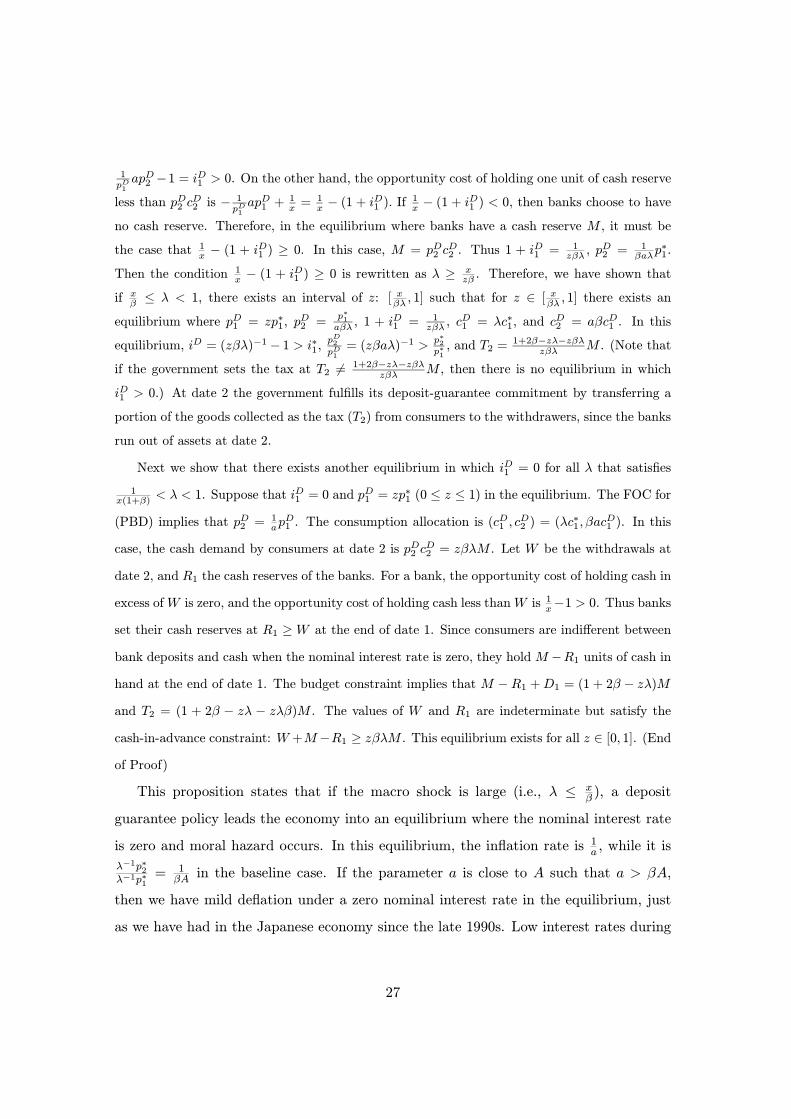
Then the condition 1x − (1 + iD1 ) ≥ 0 is rewritten as λ ≥ x

zβ . Therefore, we have shown that

if xβ ≤ λ < 1, there exists an interval of z: [ xβλ , 1] such that for z ∈ [ xβλ , 1] there exists an

equilibrium where pD1 = zp∗1, pD2 =

p∗1aβλ , 1 + i

D1 = 1

zβλ , cD1 = λc∗1, and c

D2 = aβcD1 . In this

equilibrium, iD = (zβλ)−1 − 1 > i∗1, pD2

pD1= (zβaλ)−1 > p∗2

p∗1, and T2 =

1+2β−zλ−zβλzβλ M . (Note that

if the government sets the tax at T2 6= 1+2β−zλ−zβλzβλ M , then there is no equilibrium in which

iD1 > 0.) At date 2 the government fulfills its deposit-guarantee commitment by transferring a

portion of the goods collected as the tax (T2) from consumers to the withdrawers, since the banks

run out of assets at date 2.

Next we show that there exists another equilibrium in which iD1 = 0 for all λ that satisfies

1x(1+β) < λ < 1. Suppose that iD1 = 0 and p

D1 = zp

∗1 (0 ≤ z ≤ 1) in the equilibrium. The FOC for

(PBD) implies that pD2 = 1ap

D1 . The consumption allocation is (c

D1 , c

D2 ) = (λc∗1,βacD1 ). In this

case, the cash demand by consumers at date 2 is pD2 cD2 = zβλM . Let W be the withdrawals at

date 2, and R1 the cash reserves of the banks. For a bank, the opportunity cost of holding cash in

excess ofW is zero, and the opportunity cost of holding cash less thanW is 1x−1 > 0. Thus banks

set their cash reserves at R1 ≥ W at the end of date 1. Since consumers are indifferent between

bank deposits and cash when the nominal interest rate is zero, they hold M −R1 units of cash inhand at the end of date 1. The budget constraint implies that M −R1 +D1 = (1 + 2β − zλ)Mand T2 = (1 + 2β − zλ − zλβ)M . The values of W and R1 are indeterminate but satisfy the

cash-in-advance constraint: W +M−R1 ≥ zβλM . This equilibrium exists for all z ∈ [0, 1]. (Endof Proof)

This proposition states that if the macro shock is large (i.e., λ ≤ xβ ), a deposit

guarantee policy leads the economy into an equilibrium where the nominal interest rate

is zero and moral hazard occurs. In this equilibrium, the inflation rate is 1a , while it is

λ−1p∗2λ−1p∗1

= 1βA in the baseline case. If the parameter a is close to A such that a > βA,

then we have mild deflation under a zero nominal interest rate in the equilibrium, just

as we have had in the Japanese economy since the late 1990s. Low interest rates during

27

deflation were also observed in the U.S. economy during the Great Depression.

The deposit guarantee prevents the inefficiency associated with a fire sale (or liqui-

dation) of bank assets, but at the same time this policy inevitably induces moral hazard

for banks.

4.2 Unlimited Liquidity Support

We can show that the unlimited liquidity support policy brings about welfare effects

similar to those of a deposit guarantee policy. We define the unlimited liquidity support

policy as follows. At date 1, the government declares that it will supply an unlimited

amount of liquidity on demand to banks. The government supplies cash ∆M on demand

to banks for payment to withdrawers. At the end of date 1 the banks choose efficient

or inefficient use of capital, and the consumers redeposit their cash after observing the

banks’ choice. The total cash that exists in the economy between dates 1 and 2 becomes

M +∆M . At date 2, the government collects all cash as the tax: T2 =M +∆M . Note

that this policy is not the same as the ordinary provision of liquidity by the central bank

in normal circumstances. Unlimited liquidity support involves the transfer of value from

consumers to banks by seigniorage.9 We can prove the following proposition:

Proposition 4 Suppose that π is close to zero: π ≈ 0. If

x >β

2β + 1, (18)

there is no equilibrium with a positive interest rate under the unlimited liquidity support

policy.

(Proof) We assume that iL1 > 0. In this case we can show that pL1 > p

∗1 by contradiction. Under

the liquidity support policy, the banks continue to operate at dates 1 and 2. Suppose that pL1 ≤ p∗1in the equilibrium where the interest rate is positive. Arguments similar to those of the baseline

case hold, and we have pL1 cL1 = M . The FOCs for consumers and banks under pL1 ≤ p∗1 imply

thatcL2βcL1

= A where A = A or a is the equilibrium productivity, and the resource constraint says

9The ordinary liquidity lending at the market rate of interest does not help the banks hit by the shock

λ since the difficulty they face is not only the liquidity shortage but also insolvency.

28

cL2 = A{λAK0 − cL1 }. Therefore the consumption allocation is uniquely determined as cL1 = λc∗1

and cL2 = AβcL1 , which implies pL1 = λ−1p∗1 > p∗1. This is a contradiction. Therefore, the

equilibrium price must satisfy pL1 > p∗1.

Since pL1 > p∗1, Assumption 9 implies that all depositors withdraw (1 + 2β)M at date 1.

Therefore the cash injection at date 1 is ∆M = 2βM . The lucky depositors (measure π) buy

(2β + 1)c∗1 units of the goods at p∗1, while the other can buy the goods only at p

L1 . The lucky

consumers solve

(PCπ) max u(c01) + βu(c02)

subject to pL1 c01 +D

01 ≤ (2β + 1)pL1 c∗1,

pL2 c02 + T2 ≤ (1 + iL1 )D0

1.(19)

The unlucky consumers solve

(PC1− π) maxu(c001 ) + βu(c002 )

subject to pL1 c001 +D

001 ≤ (2β + 1)M,

pL2 c002 + T2 ≤ (1 + iL1 )D00

1 .(20)

Define cL1 ≡ πc01 + (1− π)c001 , cL2 ≡ πc02 + (1− π)c002 , and D

L1 ≡ πD0

1 + (1 − π)D001 . The aggregate

budget constraint is

pL1 cL1 +D1 ≤ (2β + 1)(πpL1 c∗1 + (1− π)M),

pL2 cL2 + T2 ≤ (1 + iL1 )D1.

(21)

Banks solve max pL1 cL1 +

pL21+iL1

A{λAK0 − cL1 }. The FOCs are

cL2βcL1

=pL1pL2(1 + iL1 ) = A.

The FOCs and the budget constraint (21) imply pL(cL1 −πc∗1) = (1−π)M . Thus pL1 = 1−πλ−πp

∗1. The

FOCs and the budget constraint (21) imply that D1 =(1−π)λλ−π 2βM , and 1 + iL1 =

1+2ββ

λ−π(1−π)λ .

The conditions for the banks to set the cash reserve at pL2 cL2 are 1 + iL1 − 1 = iL1 > 0 and

1x − (1 + iL1 ) > 0. When π ≈ 0, the latter is equal to

x <β

2β + 1,

which is violated if (18) holds. (The condition (18) holds for x > .33 if β = .9.) Therefore, an

equilibrium with a positive interest rate does not exist in this case. (End of Proof)

29

This proposition states that under the unlimited liquidity support policy, the gov-

ernment provides too much cash so that no banks would hold cash in the case where

i1 > 0.

Proposition 5 Suppose that π ≈ 0. If the government sets iL1 = 0 under the unlimitedliquidity support policy, it can attain the equilibrium where there are no bank runs, but

moral hazard occurs for banks.

(Proof) First we show that if iL1 = 0, it must be the case that pL1 ≤ p∗1. Suppose that pL1 > p∗1 while

iL0 = 0. The similar arguments as in the proof of Proposition 4 imply that ∆M must be 2βM ,

and the aggregate budget constraint is (21). Setting iL1 = 0 and T2 = M +∆M = (2β + 1)M ,

we have

pL1 c∗1{(1 + β)λ− (2β + 1)π} = −(2β + 1)πM,

which implies pL1 < 0 for a small π. This is a contradiction. Therefore, pL1 ≤ p∗1 if iL1 = 0.

Next we show that there exists an equilibrium where pL1 = zp∗1 (0 < z < 1) under a liquidity

support policy that satisfies iL1 = 0. Since the government sets iL1 = 0, the price must satisfy

pL1 = zp∗1 for some z (0 < z ≤ 1). Since the government declares that it supplies an unlimitedamount of liquidity to banks, consumers and banks have the expectations that banks continue to

operate at dates 1 and 2. Thus the FOCs for the bank’s problem and Lemma 1 implycL2βcL1

= a,

and the resource constraint is cL2 = a(λAK0 − cL1 ). Therefore cL1 = λc∗1 and cL2 = βacL1 , implying

pL1 cL1 = zλM and pL2 c

L2 = βzλM . The budget constraint for consumers and T2 =M+∆M imply

∆M = {2β − (1 + β)zλ}M. (22)

In the equilibrium where i1 = 0, the values of withdrawal W and cash reserves R1 are indeter-

minate, but satisfies R1 > W and W +M −R1 ≥ zβλM . We have shown that for each z thereexists an equilibrium in which iL1 = 0, and moral hazard occurs. (End of Proof)

The above propositions state that in the equilibrium under the unlimited liquidity

provision policy, moral hazard is induced for banks, and the aggregate productivity

declines from A to a. Thus the welfare effect of the liquidity provision policy is same as

that of a deposit guarantee policy: the policy can prevent the inefficiency of a fire sale

(or liquidation) of bank assets, but it inevitably induces moral hazard for banks.

30

4.3 Bank Recapitalization

Our interest is in determining whether there exists an optimal policy that can prevent

both fire sales and moral hazard. Since moral hazard is caused by the commitment

to provide an unlimited supply of goods or liquidity when banks run short, we should

consider the type of policies in which the government supplies a fixed amount of resources

to the banks before withdrawals occur and declares that it will not supply additional

resources ex post.

In this section we examine bank recapitalization through the infusion of public funds

from this point of view. In our model, we can consider two types of bank recapitalization

policy. One is an approach that transfers value from consumers to banks by monetary

policy or seigniorage. In this case the government creates cash ∆M and gives it to the

banks at date 1, and collects all the cash in the economy (M + ∆M) by taxation on

consumers (T2 = M + ∆M) at date 2. The other type of recapitalization policy is an

approach that transfers value by fiscal policy. There are various different fiscal measures

that can be used to transfer value, but it can be easily understood that they result in

the same welfare effects within our simple model. We examine the case in which the

government issues bonds (B), gives B to the banks at date 1, and redeems the bonds by

taxation on consumers (T2 =M + (1 + i1)B).

We denote the variables in the equilibrium under the bank recapitalization policy

with superscript C: prices (pC1 , pC2 , i

C1 ) and the allocation (c

C1 , c

C2 ).

4.3.1 Case 1: Recapitalization by Monetary Policy

We examine the first type of recapitalization policy. At date 1, the government creates

cash ∆M and gives it to the banks before withdrawals occur. The government declares

that it will not provide any additional resources to the banks during or after the with-

drawals of date 1. The government levies the tax T2 =M+∆M on consumers at date 2.

We call this policy “monetary recapitalization” in the following. We prove the following

proposition.

31

Proposition 6 Suppose that π ≈ 0 and x > 23 . If the government implements monetary

recapitalization that satisfies ∆M ≥ max{(2β− (1+β)λ)M, (β− 12)M}, the equilibrium

interest rate becomes zero, and moral hazard inevitably occurs for banks.

(Proof) There are four cases10 for the equilibrium interest rate and price: (Case 1) iC1 = 0 and

pC1 ≤ p∗1, (Case 2) iC1 = 0 and pC1 > p∗1, (Case 3) iC1 > 0 and pC1 ≤ p∗1, and (Case 4) iC1 > 0 andpC1 > p

∗1.

Case 1. If iC1 = 0 and pC1 ≤ p∗1, the equilibrium outcome is same as that described in

Proposition 5. Lemma 1 implies that moral hazard occurs in this case.

Case 2. Lemma 1 also implies that moral hazard occurs in an equilibrium where iC1 = 0 and

pC1 > p∗1, if it exists.

Case 3. We show that if iC1 > 0 then pC1 cannot be less than or equal to p∗1. Suppose that

iC1 > 0. Consumers deposit their all assets in banks, and they do not hold cash. The banks hold

M+∆M units of cash as the reserves. Suppose that pC1 ≤ p∗1 in this case. If pC1 ≤ p∗1, no depositorswithdraw their entire deposits at date 1. Therefore the budget constraint for consumers becomes

pC1 cC1 +D1 ≤ (1 + 2β)M , and pC2 cC2 + T2 = (1 + iC1 )D1. Since iC1 > 0 the opportunity cost for

banks to hold cash in excess of date-2 withdrawals is positive. The opportunity cost for banks to

hold cash less than date-2 withdrawals is 1x −(1+ iC1 ). Suppose that 1x −(1+ iC1 ) < 0. In this caseno banks hold cash and so there is no equilibrium where iC1 > 0. Thus in the equilibrium where

iC1 > 0, it must be the case that1x −(1+ iC1 ) ≥ 0, which impliesM +∆M = pC2 c

C2 . Since a bank’s

liability must be equal to its assets at date 2, (1 + iC1 )D1 = pC2 c

C2 +M +∆M . The FOCs for the

consumer is pC2 cC2 = (1 + iC1 )βp

C1 c

C1 . All these equations imply p

C1 c

C1 = M . Since cC1 = λc∗1 in

the equilibrium where bank runs do not occur at date 1, the price pC1 =Mλc∗1

> Mc∗1= p∗1. This is

a contradiction. Thus, in the equilibrium where iC1 > 0, it must be the case that pC1 > p

∗1.

Case 4. We show that there is no equilibrium in which iC1 > 0 and pC1 > p

∗1. Suppose that

iC1 > 0 and pC1 > p

∗1 in the equilibrium. In this case, all depositors try to withdraw their entire

deposits (1+ 2β)M . If ∆M ≥ 2βM , the outcome is the same as that described in Proposition 4.Thus in the case where ∆M ≥ 2βM , there is no equilibrium. (Note that Proposition 5 impliesthat the equilibrium with iC1 = 0 exists only if ∆M < 2β.) If (β − 1

2 )M ≤ ∆M < 2βM , the

banks can pay (2β + 1)M to the depositors at date 1 by selling a portion of their assets in a

fire sale. In this case, the aggregate budget constraint for the consumers is similar to (21) since

10Note that there is no disintermediation, since M +∆M ≥ (β + 12 )M , which implies that banks can

repay all depositors in full if they sell (a portion of) their assets in a fire sale.

32

iC1 > 0:

pC1 cC1 +D1 ≤ (2β + 1)(πpC1 c∗1 + (1− π)M),

pC2 cC2 + T2 ≤ (1 + iC1 )D1.

(23)

In this equilibrium it must be the case that

1

x− (1 + iC1 ) ≥ 0, (24)

since otherwise no banks hold cash. We will clarify the condition for (24) later. Assuming that

(24) is satisfied, we have pC2 cC2 =M+∆M . The FOC for the consumer is pC2 c

C2 = β(1+ iC1 )p

C1 c

C1 .

Therefore

pC1 cC1 =

½pC1p∗1π + 1− π

¾M. (25)

Since ∆M is predetermined, the withdrawal of (1 + 2β)M causes a partial fire sale of the bank

assets, which produces a deadweight loss of (1−x)(2βM−∆M)

xpC1units of the consumer good. Therefore

in this equilibrium

cC1 =1

1 + β

½λAK0 − (1− x)(2βM −∆M)

xpC1

¾. (26)

The equations (25) and (26) imply

pC1p∗1=1− πλ− π +

1− xx

2βM −∆M(1 + β)M(λ− π) . (27)

Now we examine the condition for (24). Since equation (27) and pC2 cC2 = β(1 + iC1 )p

C1 c

C1 , (24) is

rewritten as

∆M

M≤

1−πλ−πλ+

1−xx

2βπ(1+β)(λ−π) − x

β

xβ+ 1−x

xπ

(1+β)(λ−π). (28)

Since the condition (28) does not hold for ∆M that satisfies (β − 12 )M ≤ ∆M < 2βM if π ≈ 0

and x > 23 , there exists no equilibrium in which iC1 > 0 and p

C1 > p

∗1.

The above analysis on Cases 1—4 implies that the equilibrium interest rate under monetary

recapitalization must be zero, and thus moral hazard occurs in the equilibrium. (End of Proof)

The analysis on Case 4 implies that monetary recapitalization provides too much

cash so that 1x − (1 + i1) < 0 holds and banks are unwilling to hold cash reserves. To

have 1x − (1 + i1) > 0, the government must supply insolvent banks non-cash assets.

4.3.2 Case 2: Recapitalization by Fiscal Policy

The second type of recapitalization is the following: At date 1, after the shock λ hits

the economy, the government issues bonds amounting to B, and gives this amount to

33

the banks before withdrawals occur. The government declares that it will not provide

any additional resources to the banks during or after the withdrawals of date 1. The

government levies the tax T2 =M+(1+iC1 )B on consumers at date 2. We call this policy

“fiscal recapitalization.”11 We assume that the government bond B has the same return

profile as a bank deposit, and that the sale of the bonds does not result in a deadweight

loss, unlike a fire sale of consumer goods.

Assumption 13 The government bond B issued at date 1 yields (1+ iC1 )B units of cash

at date 2. The bond B is exchangeable for B units of cash at date 1. When the banks sell

the bond at date 1 and pay the proceeds of the bond sale to the depositors on the same

date, they do not incur the deadweight loss as associated with a fire sale of consumer

goods.

This assumption states that government bonds and bank deposits are equivalent assets

for consumers. The latter part of the assumption is just for simplicity of exposition:

we can derive qualitatively identical results even if a fire sale of the bonds generates a

deadweight loss.

Proposition 7 There exists a fiscal recapitalization policy that supports the optimal equi-

librium in which pC1 ≤ p∗1, iC1 > 0 and both fire sales of the goods and moral hazard forthe banks are prevented.

(Proof) It is sufficient to examine the case where iC1 > 0 (Lemma 1). We derive the conditions

for B that induce the optimal equilibrium, where fire sales and moral hazard are prevented.

We derive the condition for pC1 ≤ p∗1 in the equilibrium where iC1 > 0. Suppose that pC1

exceeds p∗1. Then all depositors try to withdraw (2β + 1)M . Since the banks’ cash reserve is M ,

and the banks can obtain cash M by selling all their assets, the total cash that the banks can

pay to the depositors is 2M , which is less than (2β + 1)M . Therefore if pC1 > p∗1, the banks go

11There are several other fiscal measures to recapitalize the banks. For example, the government can

tax consumers at date 1 and transfer the tax revenue (i.e., cash or goods) to the banks on the same date,

or it can issue bonds, sell them to consumers, and give the proceeds of the bond sale (i.e., cash) to the

banks on date 1. It is easily confirmed that these policies have the same welfare effect as the above fiscal

recapitalization policy.

34

bankrupt, and pC1 is determined by

pC1 =M

λxAK0 +BpC1

. (29)

Since no production technology is available in this case (see Assumption 12), the equilibrium

after disintermediation would be the solution to

maxc1,s,M1,B1,c2

u(c1) + βu(c2)

subject to pC1 c1 + p

C1 s+M1 +B1 ≤ pC1 λxAK0 +B +M,

pC2 c2 + T2 ≤ pC2 s+M1 + (1 + iC1 )B1,

pC2 c2 ≤M1,

(30)

where T2 =M + (1 + iC1 )B. In the disintermediated economy, the nominal interest rate iC1 is set

to satisfy 1 + iC1 =pC1pC2since the only asset is the consumer good that is stored; one unit of cash

is transformed into 1pC1units of the consumer goods at date 1, whose return is

pC2pC1units of cash

at date 2. As in the case of equilibrium after debt deflation (page 23), it is easily shown that

pC2 =∞ and (c1, s, c2,M1, B1) = (λxAK0, 0, 0,M,B) in the equilibrium after disintermediation;

each consumer stores cash (M) and bonds (B), and pays them to the government as the tax

T2 =M + (1 + iC1 )B =∞.If the government sets B such that

B ≥ {1− λx(1 + β)}M, (31)

then the equation (29) implies that pC1 =M−BλxAK0

≤ p∗1. Therefore, if the government sets B to

satisfy (31), the price in disintermediation (pC1 ) must be no greater than p∗1. So we assume that

the government sets B in such a way. Since pC1 ≤ p∗1 in this case, there are no depositors whomake runs on banks in the equilibrium. Thus the aggregate budget constraint is

pC1 cC1 +D1 ≤ (1 + 2β)M,

pC2 cC2 + T2 ≤ (1 + iC1 )D1.

(32)

Since iC1 > 0, the opportunity cost for the banks to hold cash reserves in excess of the date-2

withdrawal (pC2 cC2 ) is i

C1 > 0, while the opportunity cost for the banks to hold cash reserve less

than pC2 cC2 is

1x − (1 + iC1 ). We will verify later that

1

x− (1 + iC1 ) > 0. (33)

35

Assuming that (33) holds, we have pC2 cC2 = M . The FOC for the consumers implies pC2 c

C2 =

β(1 + iC1 )pC1 c

C1 . Since T2 =M + (1 + iC1 )B, we have

pC1 cC1 =M −

B

2β + 1. (34)

Since there is no fire sale when pC1 ≤ p∗1, the FOCs and the resource constraint imply cC1 =

11+βλAK0 = λc∗1. If the government sets

B ≡ (2β + 1)(1− z)M ≥ (2β + 1)(1− λ)M, (35)

the equilibrium price pC1 = zλMc∗1= z

λp∗1 ≤ p∗1. We have shown that by setting z ≤ λ, the

government can induce a situation where pC1 ≤ p∗1 and prevent fire sales.We will now examine the condition for z (or B) to prevent moral hazard. Suppose that a bank

offers its depositors to renegotiate at date 1 after it forms its capital of λAK0 − cC1 . The bank’sliability isD1 = (1+2β)M−pC1 cC1 = (1+2β)M−zM , while its assets areM units of cash, B units

of the bond, and λAK0−cC1 = βcC1 units of capital. The amount of cash that the bank can collect

by selling the bonds and the goods in a fire sale isM+B+xpC1 βcC1 =M+(1+2β)(1−z)M+βxzM .

This amount is less than the bank’s liability if

1 ≤ zβ(2− x). (36)

If (36) holds, the bank’s offer of renegotiation results in the bankruptcy of the bank at date 1.

Therefore the banks never try to renegotiate if (36) holds. In this case cC2 = βAcC1 = βAλc∗1,

pC2 = McC2, and 1 + iC1 = 1

βz ≤ 2 − x. Now we verify (33): 1x − (1 + iC1 ) ≥ 1

x + x − 2 > 0 for

0 < x < 1. Thus if B satisfies (31), (35), and (36), then the equilibrium in which iC1 > 0 is

uniquely determined for a fixed value of B. The sufficient condition for the existence of such B

is

0 < Z ≡ min½λx(1 + β) + 2β − 1

1 + βx,3β − 1

2 + λx(1 + β)

1 + 2β

¾. (37)

Obviously this condition (37) is satisfied, since the discount factor β is larger than 16 . Therefore

the government can pick z that satisfies 0 ≤ z < Z, and set B = (1 + 2β)(1 − z)M . In thisequilibrium, both the fire sale and moral hazard are prevented, and the optimal consumption

allocation is realized. (End of Proof)

This result appears to be quite different from that of Diamond and Rajan (2002b),

who claim that recapitalization of failing banks during a financial crisis may worsen the

crisis. Diamond and Rajan (2002b) seem to use the term “recapitalization” to represent

36

a policy that transfers liquidity to an insolvent bank from other banks. Thus in their

model, the amount of aggregate liquidity does not increase at date 1, and therefore bank

bailouts result in more inefficient liquidation of bank assets. This outcome seems similar

to that of a deposit guarantee in our model (Lemma 2).

In the fiscal recapitalization policy of our model, however, the government can create

aggregate liquidity when it recapitalizes insolvent banks by issuing government bonds,

which can be sold in the market at date 1: The government bond in our model is

accepted as a liquid asset by consumers. Thus in our model, fiscal recapitalization solves

the problems of both insolvency and illiquidity. Diamond and Rajan (2002a) also state

that capital injections can provide better outcomes when combined with injections of

liquidity.

Propositions 5 and 6 imply, however, that cash injections alone are not sufficient

to attain the optimal allocation. This is because the increase in the money supply

distorts the decision making of banks through the cash-in-advance constraint, while fiscal

recapitalization can avoid this distortion.12

5 Conclusion

When the economy is hit by a macroeconomic shock that makes the banking system

insolvent and thus raises the risk of debt deflation, different policy responses have quite

different welfare effects.

A deposit guarantee, unlimited liquidity support, and monetary recapitalization gen-

erate inefficient outcomes. Fiscal recapitalization is the optimal policy that can prevent

both moral hazard (inefficient use of capital) at banks and the premature liquidation of

bank assets. In crisis-hit countries, policies of temporization, such as a deposit guaran-

tee and unlimited liquidity support, are often adopted. Our results imply that a deposit

12Boyd, Chang, and Smith (2000) argue that to monetize the cost of bank bailouts is better than

taxation. In their model, cash is introduced by the reserve requirement imposed by the government, and

it does not induce moral hazard for banks as it does under a zero nominal interest rate in our model (See

Lemma 1). Therefore, monetization is not inefficient in their model, while it is in ours.

37

guarantee and unlimited liquidity support may give rise to a combination of mild de-

flation and low interest rates (Propositions 3, 5, and 6). Our results also imply that

temporizing without recapitalizing insolvent banks causes a larger welfare loss. These

implications are consistent with the observations on recent financial crises that we refer

to in Section 1.

Let us examine the Japanese economy of the 1990s in our theoretical framework.13

Although Japan experienced a full-fledged crash of its asset-price bubble at the beginning

of the 1990s, the government did not begin to recapitalize major banks until 1998; during

the 1990s the government insisted that it would never allow the occurrence of a bank

closure; meanwhile, the central bank has kept the short-term interest rate at zero since

1995. This attitude of the Japanese government can be interpreted as employing the

policy of a deposit guarantee14 and liquidity support.15 The decade-long stagnation of

the Japanese economy seems consistent with the predictions of our model. The deflation

since the late 1990s can also be interpreted as a result of the implementation of a deposit

guarantee without sufficient recapitalization.

In short, Japan’s prolonged recession and current deflation may have been caused by

an inappropriate policy response to bank insolvency: temporization with “too little and

too late” recapitalization.

13We can easily generalize this two-period model into a multi-period model preserving the intuition

so that the basic implication of the model can be applied to the decade-long recession of the Japanese

economy.14Although Japan established a deposit insurance system in the 1970s that guarantees up to 10 million

yen for any single depositor, there was a tacit understanding that the government would never let any

bank close, meaning in practice that deposits were guaranteed without limit. In 1995, the government

declared explicitly that it would guarantees all deposits without limit for the time being. This unlimited

deposit guarantee has still not been eliminated as of 2003.15The monetary easing by the Bank of Japan was very aggressive, but it turned out that the speed

and the scale of the monetary policy were insufficient. The BOJ’s intension was to provide temporary

liquidity support but not to subsidize the insolvent banks by seigniorage. Therefore, the monetary policy

in the 1990s was insufficient for the restoration of bank solvency.

38

References

Alexander, W. E., J. M. Davis, L. P. Ebrill, and C. - J. Lindgren, eds. (1997). Systemic

Bank Restructuring and Macroeconomic Policy, International Monetary Fund.

Allen, F., and D. Gale (1998). “Optimal Financial Crises,” Journal of Finance 53

(4):1245—84.

– (2000). “Bubbles and Crises,” The Economic Journal 110:236—56.

– (2001). “Financial Fragility,” Wharton Financial Institutions Center Working Paper

01-37, University of Pennsylvania.

Bergoeing, R., P. J. Kehoe, T. J. Kehoe, and R. Soto (2002). “Policy-Driven Productivity

in Chile and Mexico in the 1980’s and 1990’s,” American Economic Review (Papers and

Proceedings) 92 (5): 16—21.

Bordo, M., B. Eichengreen, D. Klingebiel, and M. S. Martinez-Peria (2001). “Is The

Crisis Problem Growing More Severe?,” Working Paper, World Bank.

Boyd, J. H., P. Gomis, S. Kwak, and B. D. Smith (2001). “A User’s Guide to Banking

Crises,” mimeo.

Boyd, J., C. Chang, and B. D. Smith (2000). “Deposit Insurance and Bank Regulation

in a Monetary Economy: a General Equilibrium Exposition,” mimeo.

Burnside, C., M. Eichenbaum, and S. Rebello (2001). “Prospective Deficits and the

Asian Currency Crisis,” Journal of Political Economy 109: 1155—97.

39

Caprio, G., Jr., and D. Klingebiel (1996). “Bank Insolvency: Bad Luck, Bad Policy,

or Bad Banking?,” Paper presented at Annual World Bank Conference on Development

Economics 1996.

– (1999). “Episodes of Systemic and Borderline Financial Crises,” World Bank, mimeo.

Claessens, S., D. Klingebiel, and L. Laeven (2001). “Financial Restructuring in Banking

and Corporate Sector Crises: What Policies to Pursue?,” NBER Working Paper 8386.

Diamond, D., and P. Dybvig (1983). “Bank Runs, Deposit Insurance, and Liquidity,”

Journal of Political Economy 91: 401—19.

Diamond, D., and R. G. Rajan (2001). “Liquidity Risk, Liquidity Creation, and Financial

Fragility: A Theory of Banking,” Journal of Political Economy, 109(2): 287—327.

– (2002a). “Liquidity Shortages and Banking Crises,” NBER Working Paper 8937.

– (2002b). “Bank Bailouts and Aggregate Liquidity,” American Economic Review (Pa-

pers and Proceedings) 92 (5): 38—41.

Fisher, I (1933). “The Debt-Deflation Theory of Great Depressions,” Econometrica 1

(4): 337—57.

Freixas, X., B. Parigi, and J.-C. Rochet (1999). “Systemic Risk, Interbank Relations

and Liquidity Provision by the Central Bank,” mimeo.

Grossman, S., and L. Weiss (1983). “A Transactions-Based Model of the Monetary

Transmission Mechanism,” American Economic Review 73, 871—80.

40

Honohan, P. (2001) “Recapitalizing Banking Systems: Implications for Incentives and

Fiscal and Monetary Policy,” Working Paper, World Bank.

Honohan, P., and D. Klingebiel (2000). “Controlling Fiscal Costs of Banking Crises,”

Policy Research Working Paper 2441, World Bank.

Loewy, M. B. (1991). “The Macroeconomic Effects of Bank Runs: An Equilibrium

Analysis,” Journal of Financial Intermediation 1:242—56.

Martin, A. (2001). “Liquidity Provision vs. Deposit Insurance: Preventing Banking

Panics without Moral Hazard?, ” Working Paper, Research Division, Federal Reserve

Bank of Kansas City.

Postlewaite, A., and X. Vives (1987). “Bank Runs as an Equilibrium Phenomenon,”

Journal of Political Economy, 95(3): 485—91.

Smith, B. D. (2002). “Monetary Policy, Banking Crises, and the Friedman Rule.” Amer-

ican Economic Review (Papers and Proceedings) 92 (5): 128—34.

Sargent, T. J. (1987). Macroeconomic Theory, Academic Press.

41