DEBT AMORTIZATION AND SIMPLE INTEREST: THE CASE OF ...oaji.net/articles/2014/1191-1417448053.pdf ·...

85

Recebido em 07.04.2014. Revisado por pares em 20.07.2014. Reformulado em 20.08.2014.

Recomendado para publicação em 31.08.2014. Publicado em 01.12.2014.

Licensed under a Creative Commons Attribution 3.0 United States License

DEBT AMORTIZATION AND SIMPLE INTEREST: THE CASE OF PAYMENTS IN

AN ARITHMETIC PROGRESSION

AMORTIZAÇÃO DE DÍVIDAS E JUROS SIMPLES: O CASO DE PRESTAÇÕES

EM PROGRESSÃO ARITMÉTICA.

AMORTIZACIÓN DE DEUDAS E INTERESES SIMPLES: EL CASO DE

PAGAMENTOS EN PROGRESIÓN ARITMÉTICA.

Clovis José Daudt Lyra Darrigue de Faro

Pós-Doutor pela Universität München

Doutor em Engenharia Industrial (Stanford University)

Professor da Fundação Getulio Vargas (FGV)

Endereço: Praia de Botafogo, 190 - 11º andar – Botafogo

22.253-900 - Rio de Janeiro/RJ, Brasil

Email: [email protected]

ABSTRACT

With the argument that, necessarily, compound interest implies anatocism, the Brazilian

Judiciary has been determining that, specially for the case of debt amortization in accordance

with the so called Tabela Price, when we have constant payments, simple interest must be

used. With the same determination occurring in the case of the Constant Amortization

Scheme, when the payments follow arithmetic progressions. However, as simple interest

lacks the property of time subdivision, it is shown that, as in the case of constant payments,

the adoption of simple interest in the case of payments following an arithmetic progression

results in amortization schemes that are financially inconsistent. In the sense that the

determination of the outstanding principal in accordance with the prospective, retrospective

and of recurrence methods lead to conflicting results. To this end, four different variations of

the use of simple interest are numerically analyzed.

Key words: Amortization; Simple Interest; Compound Interest

RESUMO

Com base no argumento de que, necessariamente, o regime de juros compostos implique em

anatocismo, o nosso Judiciário tem determinado que, especialmente no caso de amortização

de empréstimos segundo a chamada Tabela Price, onde as prestações são constantes, seja

adotado o regime de juros simples. O mesmo ocorrendo no caso do Sistema de Amortização

Constante, quando as prestações evoluem segundo progressões aritméticas. Todavia, por não

gozar da propriedade dita de cindibilidade do prazo, evidencia-se que, do mesmo modo que

no caso de prestações constantes, a adoção do regime de juros simples no caso de prestações

em progressão aritmética, resulta em sistemas de amortização que são financeiramente

inconsistentes. No sentido de que a determinação do saldo devedor apresenta resultados

conflitantes quando se consideram os métodos prospectivo, retrospectivo e de recorrência.

Isto é mostrado por meio de exemplos numéricos relativos a quatro distintas variantes.

Palavras-chave: Amortização; Juros Simples; Juros Compostos

86 Faro, 2014

Debt Amortization and Simple Interest: The Case of Payments in an Arithmetic Progression

Revista de Gestão, Finanças e Contabilidade, ISSN 2238-5320, UNEB, Salvador, v. 4, n. 3, p. 85-106,

set./dez., 2014.

RESUMEN

Basado en el argumento que, necesariamente, el régimen de intereses compuestos implica

anatocismo, el Poder Judicial Brasileño determina que, especialmente en el caso de

amortización de los préstamos según la llamada Tabela Price, donde los pagamentos son

constantes, sea adoptado el sistema de intereses simples. Lo mismo que ocurre en el caso del

Sistema de Amortización Constante, cuando los pagamentos evolucionan según progresiones

aritméticas. Sin embargo, por no contar de la supuesta propiedad llamada subdivisión de

plazo, muestra que, de la misma manera que en el caso de los pagamentos constantes, la

adopción del sistema de intereses simples en el caso de pagamentos en progresión aritmética,

resulta en sistemas de amortización que financieramente son inconsistentes. En el sentido de

que la determinación del saldo deudor presenta resultados contradictorios al considerar los

métodos prospectivo, retrospectivo y de recurrencia. Esto es mostrado por medio de ejemplos

numéricos relativos a cuatro diferentes variantes.

Palabras claves: Amortización, Intereses Simples; Intereses Compuestos.

1. INTRODUCTION

Historically, the assessment of interest against interest, a practice that in legal jargon is

termed as anatocism, has been considered not only immoral, but even illegal. Furthermore, it

is customary to associate its occurrence whenever the compound interest practice is applied.

However, while anatocism implies compound interest, the opposite is not always true.

As argued by de Faro (2013-a), there is no anatocism in any debt amortization scheme in

which, what is understood as a negative amortization, does not occur. This suggests an

apparent paradox, even when the equivalence between the principal amount of a loan and the

corresponding sequence of payments is established in accordance with the principles of

compound interest.

Notwithstanding, the issue is plagued by controversy. Several authors, such as De-

Losso, Giovannetti & Rangel (2012), Nogueira (2013), Rovina (2009) and Sandrini (2007),

contend that any debt amortization scheme based on the compound interest practice implies

anatocism, namely.

Such an understanding has led to several judicial sentences by Brazilian Courts to

determine that the system of constant payments, popularly known as “Tabela Price,” as well

as the system of constant amortization (known by the acronym SAC), both based on

compound interest, should be substituted by schemes based on simple interest.

Focusing on the case of constant payments, and making use of a concept of financial

consistency, de Faro (2013-b) has shown that while the “Tabela Price” conforms with such

concept, the same does not occur when it adopts the simple interest practice, particularly

when a peculiar variant, which has been coined as “Gauss Method”, is used.

87 Faro, 2014



set./dez., 2014.

The aim of this paper is to extend the analysis to the case of SAC, which is

characterized by the fact that payments follow an arithmetic progression.

The paper is further organized as follows. The second section states the definition of

the concept of financial consistency. This concept is founded on the proposition that any

procedure used to determine the value of the outstanding debt has to produce the same result,

regardless of the amortization scheme considered.

The third section formally shows that the SAC scheme is financially consistent.

Besides, in order to contrast with the cases of the simple interest schemes, which will be

considered, it presents a numerical example, which is termed, “standard example”.

Taking into account the intrinsic characteristic of the simple interest practice, which

lacks the property of independence of the so called focal date, when establishing the

equivalence between the amount loaned and the corresponding sequence or payments, the

fourth section considers the two focal dates which can be regarded as most common.

Furthermore, besides considering a particular variant proposed by Rovina (2009), and labeled

as SAC- JS, the case of short-term loans (which employs the concept of commercial or simple

discount), is also examined.

In the fourth section, considering the “standard example,” and following the

mathematical tradition of disproving a proposition by means of a counterexample (cf.

Gelbaum and Olmsted, 2003), it is also shown that the four cases presented, fail to satisfy the

concept of financial consistency.

The fifth and final section presents the conclusions.

2. THE CONCEPT OF FINANCIAL CONSISTENCY

Given a loan of value F, and the periodic rate of interest i, suppose that the loan has to

be amortized by a sequence of n periodic end-of-period payments. Furthermore, it is assumed

that the n payments follow an arithmetic progression with common difference R . We will

assume that 0R ; otherwise, we would already have the considered case of constant

payments.

Denoting as kP the payment due k periods after the date of the loan, which is taken to

be time zero, we assume that:

1 , 1,2,...,kP P k R k n (1)

where 0P is the value of the first payment.

88 Faro, 2014



set./dez., 2014.

As in the case of SAC, it will be assumed that .R i F n . However, R can assume

any value on the real line, as long as:

a) If R<0, as all payments should be positive, we must have

1 0 1nP P n R R P n ;

b) If R>0 , the corresponding value of P, which is determined when the values of F, R, n

and i are given, should be such that anatocism does not occur. This requirement implies that

we must have . .P i F Otherwise, the first amortization component would be negative. This

would occur, for instance, if F = 100.000, n = 2, the compound interest rate i being 20% per

period, and R=101.000. In this case, we would have P= 19.545,45 < i.F = 20.000.

In order to establish the concept of financial consistency, we will make use of the

following definitions:

kS - outstanding debt at time k, with k assumed to be the time immediately after the

payment kP is due, k = 1,2,..., n and 0 ;S F

kA - amortization component of payment kP ,

1.k kJ i S , interest component of payment kP , with

k k kP A J (2)

It is appropriate to point out that some authors, such as De-Losso, Giovannetti &

Rangel (2013) and Sandrini (2007) suggest that

(1 )k

k kA P i (2’)

with kJ being given by the difference between kP and kA .

Referring the reader to de Faro (2014), wherein a critical analysis of such suggestion is

presented, we will follow the procedure of taking kA as given by the difference between kP

and the component, more properly named parcel of due interest, 1.k kJ i S .

Accordingly, we will be following the European tradition, as in de Finetti (1969, p.

138), who names kA as “part de capitaux”, Kosiol (1973, p.75), who employs the expression

“tilgung,” and McCutcheon and Scott (1993, p.81), who adopt the term “capital repayment.”

On the other hand, American authors, such as Butcher and Nesbitt (1971, p.164), as well as

89 Faro, 2014



set./dez., 2014.

Kellison (1991, p.166), make use of the denominations “principal component” and “principal

repayment,” respectively.

We will also employ the following basic financial principles:

1- The outstanding debt at time k, is equal to the outstanding debt at time k-1,

increased of interest at the rate i, less the payment due at time k. That is:

11 , 1,2,...,k k kS i S P k n (3)

2- If there is no overdue payment, the debt is extinguished with the payment nP . That

is, 0nS .

3- Besides the determination of the outstanding debt kS by reiterated application of

relation (3), we can also adhere to any of the following three procedures:

3.1- retrospective method

The outstanding debt kS is equal to the difference between the amount F that was

loaned, and the sum of the amortization components already made. That is,

1

, 1,2,...,k

kS F A k n

(4)

Obviously, it follows that 1

n

k

k

A F

.

3.2- prospective method

The outstanding debt kS is equal to the present value, computed at the

interest rate i, of the remaining n-k payments.

3.3 method of recurrence

As it follows directly pursuant to the repeated application of relation (3), the

outstanding debt at time k, kS , can be determined by the difference between the accumulated

90 Faro, 2014



set./dez., 2014.

value of F, at the rate i, for k periods, and the accumulated value, at the same rate i, of the k

payments that have already been made.

A particular debt amortization scheme is said to be financially consistent, if the

outstanding debt kS can be uniquely determined by any one of the three methods above.

3. THE CASE OF THE SAC SCHEME

As it is widely known, cf. de Faro & Lachtermacher (2012, p.267), the adoption of the

SAC scheme of debt amortization implies that:

1 . 1 , 1,2,...,kP F i n i F k n k n (5)

That is, the sequence of payments follows an arithmetic progression with common

difference .R i F n and initial term 1 1P F i n .

Preliminarily, it should be observed that, considering the rate i as compound interest,

the equivalence between the loan amount F and the sequence of the n payments, can be easily

verified, since:

1 1 1

1

1 1 1 1 1

1 1 1 1 1 1 1 1

n n nk k k

k

k k k

n n n

P i F n i n i i k i

F n i n i i i i i n i F

(6)

Besides, it should also be noted that, as we do not have any negative amortization

(since kA F n for 1,2,...,k n ), we will not have the occurrence of anatocism, in the sense

as defined by Houaiss (2011), provided we do not have any overdue payment.

Let us now proceed to check if the concept of financial consistency is satisfied.

Considering the determination of the outstanding debt kS , by each one of the three

procedures under consideration, we have:

a) according to the retrospective method

It is easily seen that

91 Faro, 2014



set./dez., 2014.

1

. 1k

k j

j

S F A F k F n F k n

(7)

which shows that the outstanding debt decreases linearly with time.

b) according to the prospective method

1

1 1

1 1 1n n

k k

k k

k k

S P i P k R i

1

1

1 1 1 1 11

k n k n

k n

k

i R i iP R n k i

i i i

(8)

Thus, taking into account that

1 1 . .kP F i n i F k n

and

.R i F n

it follows that we will also have kS F n k n

c) according to the method of recurrence

As stated above, we should have

1

1 1k

k k

kS F i P i

(9)

To show that relation (9) implies relation (8), it is sufficient to observe that relation (6)

can be written as:

1 1

1 1k n

k

P i P i F

(6’)

Therefore, multiplying both sides by (1 )ki , it follows that

1 1

1 1 1k n

k k k

k

P i F i P i

(6”)

92 Faro, 2014



set./dez., 2014.

Consequently, we can conclude that the prospective method and the method of

recurrence lead to the same value for kS .

In summary, the SAC scheme of debt amortization is financially consistent.

As a numerical illustration, Table I shows the evolution of the outstanding debt for the

case of what is called “standard example.” In this case, we have F=R$ 100.000,00, n = 5

periods and i = 2% for period.

Taking into consideration that P1 = R$ 22.000,00 and R = -R$ 400,00, we have:

Table I

Evolution of the Outstanding Debt in the Case of SAC

k kS kP

kJ k

0 100.000,00 - - -

1 80.000,00 22.000,00 2.000,00 20.000,00

2 60.000,00 21.600,00 1.600,00 20.000,00

3 40.000,00 21.200,00 1.200,00 20.000,00

4 20.000,00 20.800,00 800,00 20.000,00

5 0,00 20.400,00 400,00 20.000,00

Totals - 106.000,00 6.000,00 100.000,00

Values in Brazilian reais

In this particular case, as a further numerical illustration, let us consider the

determination of the outstanding debt just after the date of the third payment. We have:

a) according to the retrospective method

3 100.000 1 3 5 $ 40.000,00S R

b) according to the prospective method

1 2

3 20.800 1 0,02 20.400 1 0,02 $ 40.000,00S R

c) according to the method of recurrence

3 2

3 100.000 1 0,02 22.000 1 0,02 21.600 1 0,02

21.200 $ 40.000,00

S

R

93 Faro, 2014



set./dez., 2014.

4. POSSIBLE EFFECTS OF SIMPLE INTEREST IMPOSITION

Let us suppose now that, by a judicial imposition, the periodic interest rate i has to be

of simple interest.

At this point, as a historical curiosity, it is pertinent to recall, that although simple

interest had been suggested by Wilkies (1794), currently its use for debt amortization is not

mentioned at all by illustrious authors in the German, French or English languages, such as

Kosiol (1973), de Finetti (1969), Butcher and Nesbitt (1971), and McCutcheon and Scott

(1993), or is an object of criticisms, as in Kellison (1991, p. 82-88), who points out some

inherent ambiguities.

In contrast with the case of compound interest, when the selection of the focal date is

arbitrary, it is necessary to specify a particular focal date if simple interest is adopted (cf.de

Faro, 1969, p.33).

Thus, two different focal dates will be considered in the process of writing down the

equation of equivalence between the loan F and the corresponding sequence of payments.

As in de Faro (2013-b), the two focal dates that are most significant, will be

considered, namely, the date of the loan concession, time zero, and the date of the last

payment, time n.

4.1 – Taking Time Zero as the Focal Date

Once time zero is specified as the focal date, which appears to be the most logical

selection, it is also necessary to specify the type of discount procedure that is going to be

implemented.

In practice, we have two different possibilities. Either we make use of the so called

rational discount, which applies the classical simple interest formula, or we make use of

commercial discount, since the latter is used for the case of short-term loans, mainly by

banks.

4.1.1- The Case of Rational Discount

94 Faro, 2014



set./dez., 2014.

If the periodic rate i is taken to be of simple interest, and the values of F, n and R are

given, the value of the first payment, denoted by 1P , is such that:

1

1 1

1

1 . 1 .

n nk

k k

P k RPF

k i k i

(10)

As shown on Table II, which considers up to five payments, the analytical expression

for 1P becomes increasingly complex as n is increased.

Table II

Analytical Expression for 1P

n 1P

2

2 3 2 2

2 3 4 2 3 2 3

2 3 4 5 2 3 4

2 3 4

1

1 3 2 1 2 3

1 6 11 6 3 10 7 3 12 11

1 10 35 50 24 6 40 80 46 4 30 70 50

1 15 85 225 274 120 10 110 420 646 326

5 60 255 450 274

F i

F i i R i i

F i i i R i i i i

F i i i i R i i i i i i

F i i i i i R i i i i

i i i i

On the other hand, the numerical value of 1P can be easily determined, by employing

very simple recursive procedures:

If we define

1

1

1 .k k i

(11)

and

1

1

1 .k

k

k i

(12)

let

1 1 1 . , = 2,3, ..., i n (13)

and

1

2

3

4

5

95 Faro, 2014



set./dez., 2014.

1 1 1 . , = 2, 3,..., i n (14)

It follows that

1 . n nP F R (15)

Considering the “standard example,” and fixing R = - R$ 400,00, as in the

case of SAC, it is easily verified that 1P =R$ 21.969,80.

In Table III, where the values are in Brazilian reais, and applying relation (3) for

determining the value of the outstanding debt kS , we have the evolution of the

corresponding values of kS , kP , 1.k kJ i S , and k k kA P J .

Table III

Evolution of the Outstanding Debt for the Case of Rational Discount

k kS kP kJ k

0 100.000,00 - - -

1 80.030,20 21.969,80 2.000,00 19.969,80

2 60.061,00 21.569,80 1.600,60 19.969,20

3 40.092,42 21.169,80 1.201,22 19.968,58

4 20.124,47 20.769,80 801,85 19.967,95

5 157,16 20.369,80 402,49 19.967,31

Totals - 105.849,00 6.006,16 99.842,84

It should be stressed that the debt is not fully paid even after the last payment is made.

The total amortization of R$ 99.842,84 is less than the loan amount.

Besides, we have different values for the outstanding debt when we make use of the

prospective and recurrence procedures. This can be seen, for instance, if we try to determine

the value of 3S .

a) according to the prospective method

96 Faro, 2014



set./dez., 2014.

3 20.769,80 / (1 0,02) 20.369,80 / (1 2 0,002) $39.948,90S R

b) according to the method of recurrence

3 100.000(1 3 0,02) 21.969,80(1 2 0,02) 21.569,80(1 0,02)

- 21.169,80 = R$ 39.980,41

S

Consequently, we can conclude that the imposition of simple interest, using the

rational discount procedure, and taking time zero as the focal date, lead to a financially

inconsistent scheme of debt amortization.

4.1.2- The Case of Commercial Discount

Considering the case of a short-term loan, observing that we must have 1/n i , if we

denote by ˆkP the k-th payment, the adoption of the commercial discount mechanism implies

that we must have:

1

1 1

ˆ ˆ1 . 1 1 .n n

k

k k

F P i k P k R i k

(16)

For the determination of the value of the first payment 1P , we must recall not only the

expression of the sum of the n first natural numbers, given by 1 / 2n n , but also of

the sum of their respective squares, given by ( 1)(2 1) / 6n n n .

It follows that, given F, n, i and R, we have:

2

1ˆ 2 . 3 1 2 1 6 2 1P F n R n i n n i n (17)

Thus, considering the case of the “standard example,” and fixing, once more R=- R$

400,00, we infer the first payment to be 1ˆ $ 22.059,57P R .

Noticing that the above value is greater than the corresponding one in the case of SAC,

Table IV shows the evolution of the outstanding debt ˆkS (values being expressed in Brazilian

reais), when applying relation (3), as well as 1ˆ ˆˆ ˆ ˆ ˆ, . and k k k k k kP J i S A P J .

97 Faro, 2014



set./dez., 2014.

Table IV

Evolution of the Outstanding Debt in the Case of Commercial Discount

k ˆkS

ˆkP ˆ

kJ Ak

0 100.000,00 - - -

1 79.940,43 22.059,57 2.000,00 20.059,57

2 59.879,67 21.659,57 1.598,81 20.060,76

3 39.817,69 21.259,57 1.197,59 20.061,98

4 19.754,48 20.859,57 796,35 20.063,22

5 -310,00 20.459,57 395,09 20.064,48

Totals - 106.297,85 5.987,84 100.310,01

In this case, as we have a situation where ˆk kP P , for k =1,2,3,4 and 5, it follows that

one has to pay more than the value of the loan.

Furthermore, considering, for instance, the determination of 3S , we have:


3ˆ 20.859,57 1 0,02 20.459,57 1 2 0,02 $ 40.083,57S R


3ˆ 100.000 1 3 0,02 22.059,57 1 2 0,02 21.659,57 1 0,02

21.259,57 $ 39.705,72

S

R

However, an incongruity should be highlighted. While future values are being

determined in accordance with the principle of rational discount, present values are being

computed following the commercial discount procedure. Notwithstanding, the above

difference persists even if future values, N, were determined, starting with present values, V,

making use of the reciprocal relation N = V/(1-i.n). If this is taken into account, the method of

recurrence would lead to the value

98 Faro, 2014



set./dez., 2014.

3ˆ 100.000 1 3 0,02 22.059,57 1 2 0,02

21.659,57 1 0,02 21.259,57 $ 40.043,09

S

R

In any event, it is clear that the practice of commercial discount also yields a

financially inconsistent scheme of debt amortization.

4.2 – Taking the Date of the Last Payment as the Focal Date

In this case, in which, when considering constant payments, we have what has been

denominated as the “Method of Gauss” (cf. Antonick & Assunção, 2006, and Nogueira,

2013), the equation of equivalence between the loan F and the sequence of payments, kP, for

1,2,...,k n , is written as:

1

1 . 1n

k

k

F i n P i n k

or

1

1

1 . 1 1n

k

F i n P k R i n k

(18)

Therefore, given the values of F, n, i and R, and taking into account the expressions of

the sum of the first n natural numbers, and of the sum of their respective squares, it follows

that:

1 2 1 . . 3 1 2 3 6 2 1P F i n n R n i n n n i n (19)

Thus, in the case of the “standard example”, and fixing once more R = - R$

400,00, we have 1P= R$ 21.938,46.

In Table V, still making use of relation (3) for the determination of the

outstanding debt kS, the evolution of 1, , and of . and k k k k k k kS P J i S A P J

is

shown ( values in Brazilian reais).

99 Faro, 2014



set./dez., 2014.

Table V

Evolution of the Outstanding Debt Taking Time n as the Focal Date

k kS kP

kJ kA

0 100.000,00 - - -

1 80.061,54 21.938,46 2.000,00 19.938,46

2 60.124,31 21.538,46 1.601,23 19.937,23

3 40.188,34 21.138,46 1.202,49 19.935,97

4 20.253,64 20.738,46 803,77 19.934,69

5 320,26 20.338,46 405,07 19.933,39

Totals - 105.692,30 6.012,56 99.679,74

Now, as in the case when rational discount is used and time zero is considered as the

focal date, the debt is not extinguished even after the last payment is made. While this fact is

sufficient to conclude that we do not have a financially consistent debt amortization scheme,

let us also apply the prospective method as well as the recursive method for the determination

of 3S . Therefore:


3 20.738,46 1 0,02 20.338,46 1 2 0,02 $ 39.888,04S R


3 100.000,00 1 3 0,02 21.938,46 1 2 0,02

21.538,46 1 0,02 21.138,46 $ 40.076,31

S

R

It is thus clear that this type of the “Method of Gauss” approach is also financially

inconsistent.

4.2.1- A Variation : the SAC – JS

In Rovina (2009), a variation for the case of taking time n as the focal date, identified

by the acronym SAC-JS, was proposed. It was stated that the aim of this variation was to

100 Faro, 2014



set./dez., 2014.

reach a compromise between the SAC scheme and the simple interest practice, which led to

the suffix, JS.

Similarly to the procedure in the “Gauss Method”, the “weighted index” I was

defined as

3 . 2 . 2 3I i F n n i i (20)

in such a way, that the k-th component of interest is considered to be reached by

1 , 1,2,...,kJ n k I k n (21)

Then, as in the case of SAC, the specification of a constant component of amortization

implies that the k- th payment can be formulated as:

1 , 1,2,...,kP F n n k I k n (22)

Observing that the equation of value

1

1 . 1n

k

k

F n i P i n k

(23)

is satisfied, it follows that the sequence of payments forms an arithmetic progression with

constant difference R I .

It should be noted that, if .R i F n , as .i F n I , if 1n , the payments kP

decrease more rapidly than the payments kP . Therefore, for given values of n and i, noticing

that in both cases the equation of equivalence between F and the corresponding sequence of

payments are satisfied, considering simple interest at the rate i, and n as the focal date, it

follows that 1 1 and n nP P P P .

On the other hand, with regard to the SAC scheme, as

2

1 1 2 1 2 1 3 0 if 1, P P i F n i n n we have 1 1P P . Furthermore, as

22 1 2 1 3 0 n nP P F i n n i n ,we also have n nP P . Thus, if n >

101 Faro, 2014



set./dez., 2014.

1, we can conclude that the total amount of payments is greater in the case of the SAC

scheme. A numerical comparison, in terms of the values of the first payment, is presented in

the Appendix.

Turning our attention to the question of financial consistency, let us consider once

again the case of the “standard example.”

Observing that $379,746855I R , Table VI, with values in terms of Brazilian

reais, depicts the evolution of the outstanding debt 1kS F k n , as well as the values

of , and k k kP J A .

Table VI

Evolution of the Outstanding Debt According to the SAC-JS Methodology

k kS kP kJ kA

0 100.000,00 - - -

1 80.000,00 21.898,73 1.898,73 20.000,00

2 60.000,00 21.518,99 1.518,90 20.000,00

3 40.000,00 21.139,24 1.139,24 20.000,00

4 20.000,00 20.759,49 759,49 20.000,00

5 0,00 20.379,75 379,75 20.000,00

Totals - 105.696,20 5.696,20 100.000,00

Apparently, the strict adherence to the SAC-JS methodology, conforms with the

retrospective method for determining the outstanding debt, as it extinguishes with the last

payment.

However, such a conclusion would be misleading. This is illustrated in Table VII,

where we apply relation (3), considering the values of kP , with 1.k kJ i S and

k k kA P J , which values are also expressed in Brazilian reais.

Table VII

Evolution of the Outstanding Debt Considering the Basic Relation

k kS kP kJ kA

102 Faro, 2014



set./dez., 2014.

0 100.000,00 - - -

1 80.101,27 21.898,73 2.000,00 19.898,73

2 60.184,31 21.518,99 1.602,03 19.916,96

3 40.248,75 21.139,24 1.203,69 19.935,55

4 20.294,24 20.759,49 804,98 19.954,51

5 320,37 20.379,75 405,88 19.973,87

Totals - 105.696,20 6.016,58 99.679,62

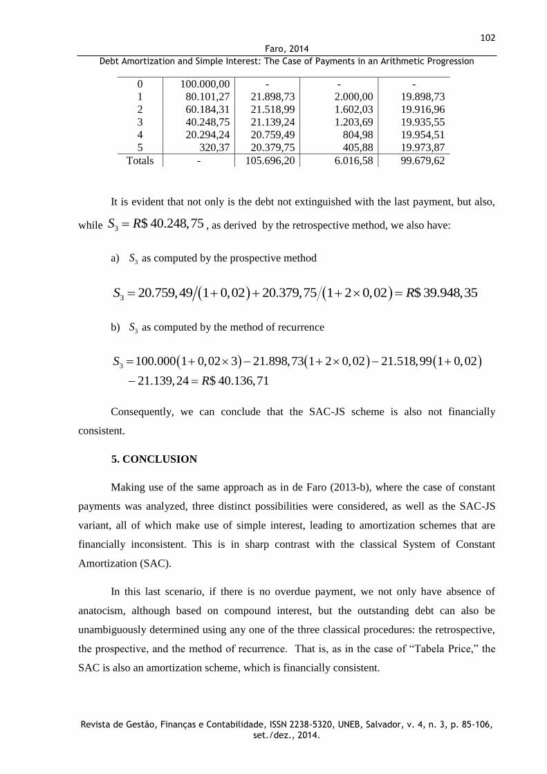
It is evident that not only is the debt not extinguished with the last payment, but also,

while 3 $ 40.248,75S R , as derived by the retrospective method, we also have:

a) 3S as computed by the prospective method

3 20.759,49 1 0,02 20.379,75 1 2 0,02 $ 39.948,35S R

b) 3S as computed by the method of recurrence

3 100.000 1 0,02 3 21.898,73 1 2 0,02 21.518,99 1 0,02

21.139,24 $ 40.136,71

S

R

Consequently, we can conclude that the SAC-JS scheme is also not financially

consistent.

5. CONCLUSION

Making use of the same approach as in de Faro (2013-b), where the case of constant

payments was analyzed, three distinct possibilities were considered, as well as the SAC-JS

variant, all of which make use of simple interest, leading to amortization schemes that are

financially inconsistent. This is in sharp contrast with the classical System of Constant

Amortization (SAC).

In this last scenario, if there is no overdue payment, we not only have absence of

anatocism, although based on compound interest, but the outstanding debt can also be

unambiguously determined using any one of the three classical procedures: the retrospective,

the prospective, and the method of recurrence. That is, as in the case of “Tabela Price,” the

SAC is also an amortization scheme, which is financially consistent.

103 Faro, 2014



set./dez., 2014.

In summary, one can conclude that, independent of the focal date, any amortization

system based on simple interest should be avoided. The imposition of simple interest may

well lead to further litigation, since the determination of the outstanding debt, a critical issue

not only in the case of anticipating the liquidation of the debt, but also when making an

extraordinary amortization, cannot be uniquely achieved.

However, disregarding the evidence presented herein, if the judiciary system persists

in imposing the implementation of amortization schemes, such as the SAC-JS, it may lead to

critical practical questions. For instance, what would happen if the liquidation of the debt

occurs before the end of the contract?

In terms of constant prices, the strict adherence to the SAC-JS methodology would

imply that, at the middle of the term of the contract, the outstanding debt would be equal to

half the value of the loan. However, taking into account the irrefutable argument that the

outstanding debt should be determined considering only the remaining payments, the debtor

may well demand the use of the prospective method. That is, the outstanding debt would have

to be computed at the present value, and at the imposed simple interest rate, of the remaining

payments.

However, as it can be inferred from the numerical example, which was presented, the

computed value would be less than half of the value of the loan. Accordingly, the SAC-JS

scheme may lead the debtor to pay more than the correct value.

Considering interest rates and terms that are effectively used in practice, a very

pertinent issue is the determination of the potential loss that may have been imposed to the

debtors.

REFERENCES

ANTONIK, Luis Roberto; ASSUNÇÃO, Marcio da Silva. Tabela Price e Anatocismo.

Revista de Administração da UNIMEP, v.4, n.1, p.120-136, jan./abr. 2006.

BUTCHER, Marjorie V.; NESBITT, Cecil J. . Mathematics of Compound Interest. Ann

Arbor: Ulrich, 1971.

DE FARO, Clovis. Matemática Financeira. Rio de Janeiro: APEC, 1969.

DE FARO, Clovis. Uma Nota Sobre Amortização de Dívidas: Juros Compostos e

Anatocismo. Revista Brasileira de Economia, v. 67, n.3, p.283-295, jul./set. 2013.

104 Faro, 2014



set./dez., 2014.

DE FARO, Clovis. Amortização de Dívidas e Prestações Constantes: uma Análise Crítica.

Ensaio Econômico da EPGE, n.746, outubro de 2013.

DE FARO, Clovis. Sistemas de Amortização: o Conceito de Consistência Financeira e Suas

Implicações, Ensaio Econômico da EPGE, nº 751, março de 2014.

DE FARO, Clovis; LACHTERMACHER, Gerson. Introdução à Matemática Financeira. Rio

de Janeiro/ São Paulo: FGV/Saraiva, 2012.

DE FINETTI, Bruno. Leçons de Mathématiques Financiéres. Paris: Dunod, 1969.

DE-LOSSO, Rodrigo; GIOVANNETTI, Bruno Cara; RANGEL, Armênio de Souza. Sistema

de Amortização por Múltiplos Contratos e a Falácia do Sistema Francês. Economic Analysis

of Law Review, v. 4, n. 1, p. 160-180, jan./jun. 2013.

GELBAUM, Bernard R.; OLMSTED, John M. H. Counterexamples in Analysis. Mineola:

Dover, 2003.

HOUAISS, Antônio. Dicionário Houaiss da Língua Portuguesa. Rio de Janeiro: Objetiva.

2001.

INSTITUTO dos MUTUÁRIOS e DEFESA dos CONSUMIDORES de PRODUTOS

FINANCEIROS. Disponível em :

http://www.imdec.com.br/fique_por_%20dentro/metodo%20graus.htm.

Acesso em 30 de outubro de 2013.

KELLISON, Stephen G. The Theory of Interest, 2 nd Ed. Homewood: Irwin, 1991.

KOSIOL, Erich. Finanzmathematik. Wiesbaden: Gabler, 1973.

McCUTCHEON, J.J.; SCOTT, W.F. An Introduction to The Mathematics of Finance. Oxford:

Butterworth – Heinemann, 1993.

NOGUEIRA, Jorge Meschiatti. Tabela Price: Mitos e Paradigmas.3.ed. Campinas:

Millenium, 2013.

ROVINA, Edson. Uma Nova Visão da Matemática Financeira: Campinas: Millenium, 2009.

SANDRINI, Jackson Ciro. Sistemas de Amortização de Empréstimos e Capitalização de

Juros: Análise dos Impactos Financeiros e Patrimoniais. Dissertação de Mestrado. Setor de

Ciências Sociais Aplicadas. Universidade Federal do Paraná, 2007.

WILKIE, David. Theory of Interest: Simple and Compound. Edimburg: P. Hill, 1794.

http://www.imdec.com.br/fique_por_%20dentro/metodo%20graus.htm.

105 Faro, 2014



set./dez., 2014.

Appendix

Numerical Comparison

Fixing F = 100.000 units of capital, and the monthly simple interest rate 2%i , the

table below presents the corresponding values of the first payments 1 1 1ˆ, , P P P and 1P

, when

R = - 2.000/n, as well as the values of 1 and P I , when the number n of payments is increased

from 1 to 360.

n 1P

1P 1P

1P R 1P I

1 102.000,00 102.000,00 102.040,82 102.000,00 - 102.000,00 -

2 52.000,00 51.990,29 52.041,24 51.980,20 1.000,00 50.986,24 986,84

3 35.333,33 35.316,24 35.379,63 35.298,47 666,67 33.982,68 649,35

4 27.000,00 26.976,18 27.052,63 26.951,46 500,00 25.480,77 480,77

5 22.000,00 21.969,80 22.059,57 21.938,46 400,00 20.379,75 379,75

6 18.666,67 18.630,29 18.733,57 18.592,59 333,33 16.979,17 312,50

7 16.285,71 16.243,34 16.360,25 16.199,46 285,71 14.550,26 264,55

8 14.500,00 14.451,77 14.582,42 14.401,87 250,00 12.728,66 228,66

9 13.111,11 13.057,15 13.201,65 13.001,37 222,22 11.311,91 200,80

10 12.000,00 11.940,42 12.098,88 11.878,90 200,00 10.178,57 178,57

11 11.090,91 11.025,81 11.198,35 10.958,68 181,82 9.251,34 160,43

12 10.333,33 10.262,82 10,.449,55 10.190,19 166,67 8.478,68 145,35

24 6.166,67 6.037,62 6.407,41 5.906,96 83,33 4.230,44 63,78

36 4.777,78 4.599,40 5.191,06 4.222,50 55,56 2.815,66 37,88

48 4.083,33 3.862.39 4.750,54 3.648,15 41,67 2.108,95 25,61

60 3.666,67 3.408,37 n.a 3.163,66 33,33 1.685,32 18,66

120 2.833,33 2.437,45 n.a 2.102,79 16,67 839,78 6.44

180 2.555,56 2.067,92 n.a 1.695,37 11,11 558,84 3,28

240 2.416,67 1.861,22 n.a 1.472,73 8,33 418,66 1,99

300 2.333,33 1.724,65 n.a 1.330,84 6,67 334,67 1,34

360 2.277,78 1.652,62 n.a 1.232,03 5,56 278,74 0,96

n.a= non applicable, as n > 1/0,02 = 50 months

It should be noted that, as . 2.000i F units of capital, values of the first payment

that are inferior to such a limit, should not be considered. Otherwise, we would have

anatocism.

106 Faro, 2014



set./dez., 2014.

Apêndice

Comparação Numérica

Fixando F = 100.000 unidades de capital, e a taxa de juros i, admitida como mensal,

em 2%, a tabela abaixo apresenta os correspondentes valores das prestações iniciais

1 1 1 1ˆ, , e P P P P

, quando 2.000 /R n , bem como os valores de 1 e de P I , para prazos n que

se estendem até 360 meses.

n

1P 1P

1P 1P R

1P

1 102.000,00 102.000,00 102.040,82 102.000,00 - 102.000,00 -

2 52.000,00 51.990,29 52.041,24 51.980,20 1.000,00 50.986,24 986,84

3 35.333,33 35.316,24 35.379,63 35.298,47 666,67 33.982,68 649,35

4 27.000,00 26.976,18 27.052,63 26.951,46 500,00 25.480,77 480,77

5 22.000,00 21.969,80 22.059,57 21.938,46 400,00 20.379,75 379,75

6 18.666,67 18.630,29 18.733,57 18.592,59 333,33 16.979,17 312,50

7 16.285,71 16.243,34 16.360,25 16.199,46 285,71 14.550,26 264,55

8 14.500,00 14.451,77 14.582,42 14.401,87 250,00 12.728,66 228,66

9 13.111,11 13.057,15 13.201,65 13.001,37 222,22 11.311,91 200,80

10 12.000,00 11.940,42 12.098,88 11.878,90 200,00 10.178,57 178,57

11 11.090,91 11.025,81 11.198,35 10.958,68 181,82 9.251,34 160,43

12 10.333,33 10.262,82 10,.449,55 10.190,19 166,67 8.478,68 145,35

24 6.166,67 6.037,62 6.407,41 5.906,96 83,33 4.230,44 63,78

36 4.777,78 4.599,40 5.191,06 4.222,50 55,56 2.815,66 37,88

48 4.083,33 3.862.39 4.750,54 3.648,15 41,67 2.108,95 25,61

60 3.666,67 3.408,37 n.a 3.163,66 33,33 1.685,32 18,66

120 2.833,33 2.437,45 n.a 2.102,79 16,67 839,78 6.44

180 2.555,56 2.067,92 n.a 1.695,37 11,11 558,84 3,28

240 2.416,67 1.861,22 n.a 1.472,73 8,33 418,66 1,99

300 2.333,33 1.724,65 n.a 1.330,84 6,67 334,67 1,34

360 2.277,78 1.652,62 n.a 1.232,03 5,56 278,74 0,96

Não aplicável, pois 1 0,02 50 mesesn .

Deve ser notado que como i.F = 2.000 unidades de capital, valores de prestação inicial

inferiores a este limite para os juros devidos não são admissíveis.

I

DEBT AMORTIZATION AND SIMPLE INTEREST: THE CASE OF ...oaji.net/articles/2014/1191-1417448053.pdf ·...

Documents

Transcript of DEBT AMORTIZATION AND SIMPLE INTEREST: THE CASE OF ...oaji.net/articles/2014/1191-1417448053.pdf ·...