Deakin Research Online This is the published version: Mills, Anthony 1995, Forecasting building price indices, Australian institute of building papers, vol. 6, pp. 121-133. Available from Deakin Research Online: http://hdl.handle.net/10536/DRO/DU:30037095 Reproduced with the kind permission of the copyright owner. Copyright : 1995, The Australian Institute of Building

Key words:

Building price index

Forecasting

Time-series

Forecasting Building Price IndicesAnthonyMillsFacultyof Architecture,Buildingand PlanningUniversityof Melbourne,Australia

AbstractThis paper examines the movement of building prices over time and the abilityof three forecasting techniques to predict future price change. The analysiswas undertaken using two time-series methods and a Delphic method in orderto predict prices on an ex-post basis.

Owing to the long lead times required to procure buildings, forecasting for atleast one year in advance is considered essential for cost planning purposes.This study analyses the ability of three independent methods to forecastchange in the Building Price Index one year in advance for the period 1987 to1994.

The results show that the time-series methods have difficulties in detectingturning points in the series, and Delphic methods, although quite accurate,produce relatively optimistic forecasts. The outcomes of the forecastingmethods were combined, producing a more accurate prediction of the BuildingPrice Index.

The results seem to suggest that an average of the forecasts produced by atime-series and an opinion survey seem to be a very accurate approach for theprediction of the Building Price Index.

IntroductionOne of the aims of building economics is to forecast accurately the tender price ofsome structure that has not yet been constructed. The lead time (or horizon) refersto the length of time into the future for which the forecast is required. Owing to thelong lead time required to design and construct buildings, forecasting of prices forat least one year in advance is considered important for cost planning purposes.

The actual duration of the design and construction phase will vary according to thesize and type of the building. However, the forecasting lead time was selectedbecause it seemed to be reasonable for cost planners to have some level ofcertainty of price movements for periods of one year in advance.

-The Building Price Index (BPI)produced quarterly by Australian ConstructionServices (ACS)has been selected as the basis of forecasting. The BPI for the period1970 to 1986 was used to develop a forecasting model. This was used to predict

/ the BPI for one year in advance over the period of 1987 to 1994.

Forecasts were analysed by comparing two time series methods and a Delphicmethod with the BPIon an ex-post basis. Forecasts were then compared with theactual BPI for the period in order to assess their accuracy.

Building prices vary between states and industries, so for this reason all priceinformation relates to non-residential construction in Victoria.

1121 Australian Institute.f Building Papers 6

Figure 1

0.2

0.15

0.1

cO0.15

c::i.Q)

"" ac:co..c

U

*' -0.05

-0.1

-0.15

-0.2

All forecasting procedures involve extending the experiences of the past into thefuture. According to Hanke (1989),they involve the assumption that conditions thatgenerated the past data are indistinguishable from the conditions of the future,except for those variables explicitly recognised by the forecasting model.

According to O'Donovan (1983).forecasting can be divided into two basic types ie,quantitative and qualitative. The qualitative methods generally use opinions toforecast future events subjectively. Quantitative forecasting methods involve theanalysis of historical data in order to produce an objective prediction of the future.All quantitative forecasting makes use of past data in order to identify a patternthat can be used to describe them. This pattern is extrapolated, or extended intothe future to make forecasts.

The Building Price IndexBuilding prices will vary owing to the fluctuation in the supply and demand forbuildings and other external factors. Although no explanation of why prices moveis given in this paper, the Building Price Index (BPI)ACS(1993) has been used asthe measure of price change in the industry. This index is widely used by costplanners in the production of cost estimates in Victoria for non-residentialconstruction.

The BPI is published monthly by Australian Construction Services, theCommonwealth government construction agency. The index is based on repricingstandard selection of building items in each state. The index used in this paper isthe 'All Works' index, which represents a cross-section of building typesconstructed by the ACS.The BPI is obtained by expressing the total of all items asa percentage of the total obtained in the base period.

For ease of understanding. building price movements are represented as thechange per annum. This is calculated by comparing two building price indicesbetween the same period over a year, ie. the percentage change in the index perannum.

Nature of Building PricesThe period from 1982 to 1994was characterised by a very large building boom inthe late 1980s, a stock market crash in 1987and a recession during the early 1990s.Building prices analysed were those applying to non-residential construction in thestate of Victoria.

Building Price Change 1983-1993

PriceMovements1983-1993.Victoria

Buildingpriceindex

Consumerpriceindex

,Implicitpricedeflator/ ' ....- ...

Quarter

11 22 Australian Institute of Building Papers 6

Figure 1 shows the movement of the BPIand the Australian Bureau of StatisticsImplicit Price Deflator for non-residential construction in Victoria. The periodchosen for analysis of the three forecasting methods extended from 1987 to 1993.

As previously stated this was a time when initially there were large volumes ofbuilding activity during the late 1980s, followed by a significant contraction inactivity levels during the early 1990s. It should be noted that significant negativeprice movement occurred between 1990to 1993.

Past Research

Past research by many authors has demonstrated the ability of times-seriestechniques to accurately predict building prices. Time-series models are based onwhat Taylor (1987)describe as 'black box' methods. Forecasts are produced on aclosed system without any attempt to understand the factors which influence thebehaviour of the system, which is done by attempting to unlock a pattern in thedata that has occurred in the past.

An important study was undertaken by Taylor (1987).which concentrated on ahierarchy of time-series analytical techniques. Each technique was used to analysethe behaviour of the BERbuilding cost index (Bureau of Economic Research,University of Stellenbosch, South Africa)

Results obtained from the application of the Box-Jenkins modelling system wereencouraging. The most appropriate model was of the Combined Auto RegressiveIntegrated Moving Average type (ARIMA)of order 2 and 1, respectively. Thismethod seem to produce the most accurate results.

In a study by Fellows (1991),the Box-Jenkins ARIMA approach was also used. Thiswas applied to the prediction of building price indices for cost adjustmentprovisions of construction contracts. It was concluded that forecasts of costescalation based upon time-series techniques offer considerable potential inpredicting cost movements.

Another important study was undertaken by Akintoye (1994),where two existingtender price forecasts were compared with a reduced-form equation modelgenerated by the authors. A series of accuracy measures was used to compareforecasts published the Building Cost Information Service, Davis Langdon &Everest and simulation out-sample forecasts made by the Akintoye and Skitmoresystem.

The study concluded that predicted values published by these organisationsbecome more variable with increasing forecasting horizons. In other words, thepredictive value of forecasts of more than a few quarters into the future diminishesrapidly. Visual observation of the BCISforecasts in the study shows quite clearlythat forecasts track the actual indices for up to two quarters. The forecasts formore than two quarters, horizons were considerably less accurate and generallydid not predict the actual turning points in price levels.

Research by Winkler (1984) in combining forecasting methods produced some veryimportant results. Winkler studies involved combining the forecasts generated bysix time-series methods. Winkler showed that the when six time-series methodswere combined, the results were more accurate than any of the individualforecasting methods. The author concluded that combining forecasts provides amore informative forecast which tends to yield smaller forecast errors.

All forecasting methods display different characteristics, but the best forecastingapproach is likely to contain elements of both quantitative and qualitative inputs.

1123 Australian Institute of Building Papers 6

Forecasting MethodsThe above studies by Taylor (1987) and Fellows (1991) demonstrated that time­series methods of forecasting provide encouraging results. Thus, two time-seriesmethods, namely Box-Jenkins ARIMA and Holt's Exponential Smoothing, have beenemployed to generate quantitative ex-post forecasts of the BPI for the periodMarch 1987 to March 1994..

In addition, results of work by Akintoye (1994), Seitz (1984) and Hanke (1989),

indicate that qualitative judgement may be necessary for medium- to long-termforecasting. Thus, the AIOS Delphic survey has been used to analyse the ability ofexperts to predict building price movements.

Box-Jenkins ARIMA Forecasting

The Box-Jenkins ARIMA method is suitable for short- to medium-range leads, butis considered to be relatively complex. However, results of earlier studies haveshown that its forecasting is of low error and may produce accurate quantitativeforecasting. ARIMA forecasts are shown in table 1.

The ARIMA Box-Jenkins methods are used to determine a model that best fits thedata under observation. This approach is a 'black box' type which does not attemptto determine the causes of movement of the indices being forecast. In fact themethod does not assume any underlying pattern in the data, and is ideal for use insituqtions where no regularity of movement is discernible.

Development of the models is complex and beyond the scope of this paper, sufficeto say that three classes of model are possible: namely Auto-Regressive (AR)type,Moving Average (MA) type and Combined Auto-Regressive Integrated MovingAverage (ARIMA).

The key to understanding ARIMA rests upon the comparison of correlationsbetween successive values of the data set (ie, auto-correlations) at various timelags. For example the auto-correlation for the BPI for a lag of one quarter would becalculated by moving the index in that lag period back by one quarter. In otherwords, auto-correlation is simply the correlation between the index at period Yowith index in period Y,. Hence, if correlation gives an indication of the strength ofrelationship between two variables, then it can be said that auto-correlation showsthe relationship between subsequent values of the same data set.

ARIMA models are of the form:

Yt = B1Yt-1+ B2Yt-2 + ... BpYt-p + et - W1et-1- W2 et-2- ... - Wq et-q

Where:Yt = independent variables that are dependent variables lagged specific timeperiodsB1, B2, Bp = regression coefficientsW1, W2, Wq = weightset = erroret-1'et-2' et-q= previous values of error

The use of ARIMA requires a stationary series, and data must not containseasonality or trend. If such a situation occurs it is common to use the first orsecond difference of tl:le series for forecasting. The general approach toforecasting is to start by using the simplest form of the model and progressivelyincrease the complexity until a satisfactory fit of the data is achieved Hanke (1989).

The following notation is frequently used with the Box-Jenkins technique. A modelis identified as ARIMA (p, d, q), where p is the order for the auto-regressive term,d is the level of differencing, and q is the order for the moving average term.

1124 Australian Institute of Building Papers 6

Various ARIMA models were tested on the BPIdata for the period 1975 to 1987 inorder to determine the best fit. The selection of the model was determined by theAkaie Information Criterion (AIC)and the most accurate forecasts were generatedby a model of the (0,2,1) type. In other words, the model that best fits the actualBPIwas a moving average of the second difference of the data. Hence the modelcan be expressed as:

Yt = Yt-1+ et - W1et-1

Where the forecast for the next period tis:Yt = et - (0.56354) et-1

Holt's Two Parameter Exponential Smoothing

Exponential smoothing is a forecasting procedure that continually revises theprediction in the light of more recent experiences. The method is based onaveraging (smoothing) past values of a series in a decreasing (exponential) manner.The observations are weighted, with more weight given to the more recentobservations. In other words, exponential smoothing is a weighted average, wherethe immediate past index is heavily weighted and has a large influence on theforecast. but the further back an index occurs the smaller the weighting becomesfor the next forecast.

A rising trend was evident in the raw BPI figures and it should be noted thatexponential smoothed forecasts will always lag behind a steadily rising or fallinglinear trend. Therefore, the trend must be estimated and the series adjustedaccordingly. One approach is two parameter exponential smoothing method (Holt).This is a combination of a simple exponential smoothing forecast which isincreased or decreased for the effect of a consistent trend.

The three equations used in the model are

Exponentially smoothed series:FH1 = AXt + (1-A)(Ft + Tt )

2 The trend estimate:TH1 = B(FH1 - Ft ) + (1-B)Tt

3 Forecast for P periods into the future:FHP = FH1+ PTH1

Where:FH1 = exponentially smoothed value in period TA = smoothing constantXt = actual value of seriesFt = average experience of series smoothed to period T-1B = smoothing constant for trend estimateTH1 = trend estimateTt = average experience of trend estimate smoothed to period TP = periods to be forecast into the futureFHP = forecast for P periods into the future

Tentative models were tested and then refined by comparing forecasts with theactual values of the BPI.Weightings were selected by minimising the meansquared error (MSE).The weighting chosen to best fit the data were A=1 andB=0.3. Forecasts are shown in table 1.

AIQS Delphic Forecasting

Delphic methods are based on an organised system of questioning individuals toelicit subjective information. The Australian Institute of Quantity Surveyorsforecasts (AIOS)is based on opinions of practising quantity surveyors, and cantherefore be considered to be of the Delphic type.

1125 Australian Institute of Building Papers 6

The survey is conducted quarterly and respondents are asked to predict the levelof building price movement for the next year. Three months later the information isreported to the AIOS respondents, at which time they are asked to make a furtherprediction for one year ahead. The figures used in this index represent the averagefirm's prediction for a 12-month period.

The collection of 12-month forecasts can therefore be compared with the annualdifference between the BPI.Alternatively, the predictions can be multiplied by theActual BPI in order to produce a one-year forecast of the BPI. Forecasts are shownin table 1.

Combined Forecasts

Past research by Winkler (1984)shows that combining forecast predictions hasmany advantage. Therefore combined forecasts were generated by calculating themean of predictions produced by other forecasting methods. Two combinationswere developed, Combination A (CA)which is the average for the forecast by theAIOS and Holt method, and Combination B (CB)which was the average of the AIOSand ARIMA method. Combined forecasts are shown in table 1.

Table 1 Forecast of BPI for Four Quarter Horizons Compared to Actual BPI

Quarter BPI AIOS HOLT ARIMA Combined A Combined B(Actual) Opinion (1) Forecast (2) Forecast (3) Average (1&2) Average (1&3)

Mar-87 778 791 808.6 816 800 804

Jun-87 793 821 831.9 835 826 828Sep-87 809 836 844.8 843 840 840

Dec-87 824 847 853.1 848 850 847Mar-88 839 887 855.3 848 871 867Jun-88 862 982 865.1 858 879 875Sep-88 862 898 878.7 874 888 886Dec-88 886 912 890.8 887 901 899Mar-89 901 930 903.7 900 917 915Jun-89 924 961 934.9 937 948 949Sep-89 932 962 913.0 904 938 933

955 982 950.5 952 966 967Mar-90 955 995 964.2 964 980 980

Jun-90 955 1012 995.8 100 1004 1006

Sep-90 955 1014 991.9 989 1003 1001

Dec-90 955 997 7024.5 7027 1071 7012

Mar-91 955 987 1003.7 996 995 991Jun-91 955 955 989.1 978 972 966Sep-97 932 926 978.8 968 953 947Dec-91 847 945 971.7 962 959 954Mar-92 809 953 966.7 959 960 956Jun-92 809 955 963.2 957 959 956Sep-92 793 915 910.1 893 973 904

Dec-92 770 835 729.7 677 782 756Mar-93 770 781 681.3 647 731 714Jun-93 755 797 719.6 717 758 757Sep-93 755 796 711.2 713 754 755Dec-93 755 780 685.2 685 733 732Mar-94 755 792 710.6 722 751 757MSE 3408 4205.0 4098 3153 3005

MAPE 0.054 0.057 0.058 0.046 0.045

I1 26 Australian Institute.f Building Papers 6

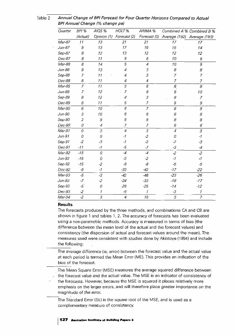
Table 2 Annual Change of BPI Forecast for Four Quarter Horizons Compared to ActualBPI Annual Change (% change pal

Ouatter BPI % AIOS% HOLT % ARIMA % Combined A % Combined B %

(Actual) Opinion (1) Forecast (2) Forecast (3) Average (1&2) Average (1&3)Mar-87 11 13 21 21 17 17Jun-87 9 13 17 16 15 14Sep-87 8 12 13 12 12 12Dec-87 8 11 9 6 10 9Mar-88 8 14 5 4 10 9Jun-88 9 13 4 3 8 8Sep-88 7 11 4 3 7 7Dec-88 8 11 4 4 7 7Mar-89 7 11 5 6 8 8Jun-89 7 12 7 8 9 70Sep-89 8 12 4 3 8 7Dec-89 8 77 6 7 9 9Mar-90 6 70 6 7 8 9Jun-90 3 10 6 6 8 8Sep-90 2 9 8 9 8 9Dec-90 0 4 7 7 6 6Mar-91 0 3 4 3 4 3Jun-97 0 0 -7 -2 0 -1

Sep-97 -2 -3 -7 -2 -2 -3Dec-97 -71 -7 -5 -7 -3 -4

Mar-92 -15 0 -4 -4 -2 -2Jun-92 -15 0 -3 -2 -7 -7Sep-92 -75 -2 -8 -8 -5 -5Dec-92 -9 -7 -33 -42 -17 -22

Mar-93 -5 -3 -42 -48 -23 -26Jun-93 -7 -2 -34 -33 -78 -17Sep-93 -5 0 -28 -25 -14 -12Dec-93 -2 1 -6 1 -3 1

Mar-94 -2 3 4 70 3 7

Results

The forecasts produced by the three methods, and combinations CA and CB areshown in figure 1 and tables 1, 2. The accuracy of forecasts has been evaluatedusing a non-parametric methods. Accuracy is measured in terms of bias (thedifference between the mean level of the actual and the forecast values) andconsistency (the dispersion of actual and forecast values around the mean). Themeasures used were consistent with studies done by Akintoye (1994) and incfudethe following:

The average difference (ie, error) between the forecast value and the actual valueat each period is termed the Mean Error (ME). This provides an indication of thebias of the forecast.

The Mean Square Error (MSE) measures the average squared difference betweenthe forecast value and the actual value. The MSE is an indicator of consistency ofthe forecasts. However, because the MSE is squared it places relatively moreemphasis on the larger errors, and will therefore place greater importance on themagnitude of the error.

The Standard Error (SE)is the square root of the MSE, and is used as acomplementary measure of consistency.

1127 Australian Institute.f Building Papers 6

Figure 2

30

20

10

«1c.gJ, 10c::

u'# 20

30

40

50

Table 3

Graph of Annual Change of BPI Forecast for Four Quarter Horizons Compared toActual BPIAnnual Change (% change pa)

AIQS4QtrOpinion

ACSBPI(ActualI/

Quarter ARIMA4QtrForecast

The Mean Absolute Percentage Error (MAPE) calculates the error as a proportion of

the variable being forecast. The MAPE considers only the absolute magnitude. Thismethod provides a measure of errors in relative terms without weighting.

The Coefficient of Variation (CV) is a relative measure of the dispersion of databetween groups. It is calculated by dividing the standard deviation of the data byits average. The CV is used to provide a consistent measure of relative dispersionbetween groups of data which have different averages, the higher the CV the

greater is the variability of the data set.

Consistency

Consistency measures the average error or difference between the forecast andthe BPI. The most common method of accuracy consistency is the MSE, SE and

MAPE and in this case each produces complementary results.

The AlaS forecasting was a consistently more accurate method than either the Holtor ARIMA forecasting method (see table 3). It had a lower MSE, SE and MAPE,indicating that the errors between the AlaS forecast and the BPI were smaller.

The Holt forecasting was consistently more accurate than ARIMA with an MSE of4099 (ARIMA 4205), SE 64.0 (ARIMA 64.8) and MAPE of 0.057 (ARIMA 0.058).

However, the methods produced very similar results and both were highlycorrelated with each other, having a co-variance of 0.0238.

The results show (table 3) that combining forecasts produced a better fit of the BPI

than any of the other methods. The Combination A (CA) forecast is the mean of theforecast for Holt and AlaS, and Combination B (CB) is the mean of ARIMA and AlaS

forecasts. The most accurate forecast was CA which was followed very closely by

the CB, and these produced consistently smaller errors over the entire period from

1987 to 1993.

Accuracy of Four Quarter Forecasts Compared to the BPI

4 Quarter ForecastsHalt ARIMA AIQS CA CB

ME (points) 26.0 19.4 45.5 35.7 32.4MSE (points) 4099.0 4205.0 3481 .7 3264.7 3112.1SE (points) 64.0 64.8 59.0 57.1 55.8MAPE(%) 5.7 5.8 5.4 4.7 4.6

11 28 Australian Institute.f Building Papars 6

Figure 3

Table 4

Bias

The first measure of bias is the ME which will indicate a trend in the forecastingerrors. It can be seen that the ME for the Alas method is significantly larger thanall the other methods. This indicates that there is likely to be a consistent bias in

the forecast.

The bias is the consistent tendency for the forecast to either underestimate oroverestimate the BPI. The Prediction-Realisation diagram Seitz (1984) has beenused to show error trends. This method is a graphical indicator which categoriseserrors in terms of their tendency to underestimate, overestimate, or to fail topredict turning points in the data.

The Prediction-Realisation for each forecast method produces a scatter diagram.The diagram plots a set of coordinates (x.y) comprising the Actual BPI percentageChange pa as 'x' and the forecast percentage change pa as 'y'. Depending onwhich sector of the graph the coordinate points fall, it will show the direction ofthe error of each forecast compared to the actual index for that period.

Prediction-Realisation of AlaS forecasts14

12

10

•8

6

4

• •2

••

-20 -15 -10 -5• • -2••• -4

ActualBPI(%Chngpal

•

5

•

•• •..., .

10 15

For instance figure 3 shows that the largest group of errors in the Alas forecastappeared in the top righthand corner, indicating that the forecast of positive changeis greater than the actual change: ie Alas forecasts overestimates positive change.The results of counting the coordinates in each sector of the Prediction-Realisationdiagram shows the direction of the error or bias of each forecast.

Sources of Forecasting Error Using Prediction-Realisation Approach

Forecast Bias AIOS HOLT ARIMASector No. % No. % No. %

Positive ChangeOverestimated 1 15 52% 5 17% 7 24%

Underestimated 2 0 0% 10 34% 8 28%Negative Change

Overestimated 4 1 3% 5 17% 4 14%Underestimated 5 5 17% 5 17% 5 17%

Fail to PredictUpturn 3 0 0% 0 0% 0 0%Downturn 6 3 10% 1 3% 2 7%

Borderline B 5 17% 3 10% 3 10%Total 29 100% 29 100% 29 100%

1129 Australian Institute 0'Building Papers 6

The PrediCtion-Realisationgraphs for the three forecasting approaches indicatesthe source of the error in the forecasting method, but do not indicate themagnitude or consistency of the error. The results show in table 4 that there is astrong tendency for the AIOS predictions to be optimistic.

Discussion

The results of three types of forecasts are now compared with the BPI in order todetermine the forecast accuracy. The trends of the 1990-1992recession had aprofound affect on the accuracy of all methods of forecasting. Visual inspection ofthe forecasts prior to 1990(figure 2) shows the accuracy of forecasting to berelatively consistent. However, from June 1991 to June 1993 the accuracy of allforecasting methods fell away significantly. This may have been due to the inabilityof the forecasting methods to predict the economic recession that occurred in theearly 1990s.

Holt's Exponential Smoothing and ARIMA forecasting

Forecasting using Holt's Exponential Smoothing and the Box-Jenkins ARIMAproduced very similar results. The Holt method produced more accurate forecastsof the BPI for four quarter ahead forecasts.

The accuracy of the forecasts was measured using the MSE between the actualforecast and the Holt and ARIMA. The results show that although both methodsproduce good forecasts of the BPI, the Holt method produces a lower MSE. Hencethe Holt method was slightly more accurate than the ARIMA method over thestudy period

However, both methods displayed similar characteristics that distinguish them as aforecasting procedure. Time-series methods such as these do not detect a turningpoint in the data ahead of its actual occurrence. Consequently, their forecasts havea tendency to overshoot both the peak and the trough of the BPI index when itchanges direction.

This is demonstrated by the extreme forecasts of a rise of 21% for both Holt andARIMA in March 1987,compared with the actual BPI for the period which showed arise of only 11%. A similar situation occurred in March 1993when the Holt andARIMA predicted prices movements of -42% and -48% respectively, compared tothe BPIwhich only showed a -5% price movement.

AIOS Delphic Forecasting

The AIOS Delphic predictions produce very accurate forecasts of building pricemovement. This somewhat surprising result showed that the MSE for AIOSforecasts were lower than either the Holt or the ARIMA methods, and hence moreconsistently accurate. This may have been due to the ability of the AIOSrespondents to pick the turning point of the 1991 recession more accurately thanthe other forecasting methods.

However, there was a tendency for the AIOS forecasts to be consistently optimisticabout future price movements. The AIOSfour quarter forecasts were in most caseshigher than the actual BPI for the period. In addition, the forecasts of price fallsduring the recession were too conservative, perhaps owing to the relativelyoptimistic outlook for improved prospects in the future.

The Prediction-Realisation method showed that during the forecasting period theAIOSforecasts were optimistic 93% of the time, and pessimistic only 7% of thetime. This contrasts markedly with the Holt and ARIMA methods that did notdisplay the same bias (see table 5).

1 130 Australian Institute of Building Papers 6

Table 5 Results of Error Source Using Prediction-Realisation Method

Forecast Character AIOS HOLT ARIMASector No. % No. % No. %

Too optimistic 1,5,6&B 27 93% 13 45% 16 55%Toopessimistic 2,3,4 &B 2 7% 16 55% 13 45%

Total 29 100% 29 100% 29 100%Too extreme 1 &4 16 55% 10 34% 11 38%Too conservative 2&5 5 17% 15 52% 13 45%Fail to predict change 3&6 3 10% 1 3% 2 7%Borderline B 5 17% 3 10% 3 10%

Total 29 100% 29 100% 29 100%

It may be reasonable to assume that professionals remain optimistic about thefuture regardless of how bleak the present economic circumstance seem to be. Ifthis is true it may explain why the AlaS opinion forecasts are mostly higher thanthe actual BPI,and rarely show negative price movements for forecasts which arefour quarters ahead.

Combining Forecasts

The combined forecasts use a simple arithmetic mean of the forecasts producedby the ARIMA, Holt and Alas Opinion methods for each four-quarter period. TheMSE for combined methods is lower than for any of the other methods, whichindicates more consistently accurate forecasting.

This result seems to confirm the work done by Winkler that by combining theoutcome of a number of forecasts the result can be much better than any of theindividual forecasts. In addition, this method combines the advantages of anobjective quantitative method with subjective human intervention.

The combination seems to produce good results because the average differencebetween quantitative forecasts and the subjective AIOS opinion varied in differentdirections from the BPI. This occurred during periods where the quantitativeforecasts were too low compared to the BPI and the AIOS too high. It should benoted that because the AIOS forecasts were more often optimistic, thecombination method will only improve error during a price downturn.

However, the combination does have the advantage during both upturn anddownturn of reducing the margin of error of the quantitative forecasts. It is obviousthat both the Holt and ARIMA forecasts produced unrealistically extreme forecasts,ie, over 20% pa in a boom and over -40% pa in a recession.

ConclusionsResults of three types of price forecasts show that there are idiosyncrasiesinherent in each method. The time-series forecasts are based on the premise thateconomic circumstances will remain stable in the future, like those of the past.Consequently, when economic conditions change the forecasting model veryquickly becomes inadequate. As a result the quantitative forecast methods areslow to react to changes in new economic circumstances.

The results of this study suggests that both the ARIMA and Holt ExponentialSmoothing methods give very similar results for four-quarter forecast horizons.However, both methods have difficulty in their ability to predict turning points inthe data, and do not detect a cyclical change in advance.

The AlaS Delphic method produces accurate forecasts. However, it contains anoptimistic bias. The results of AlaS opinions shows that there is a predisposition ofprofessionals to have a favourable view of the future. This does not seem to be

1131 Australian Instltute.f Building Papers 6

uncharacteristic of this method and has also been reported by Akintoye (1994) andMakridakis (1986). However, 'expert' professionals have also shown that they canforecast very accurately and do not seem to make excessively extreme predictionsat any time during the study period.

Different forecasting methods independently produce different results, and in onesense it is fair to say that each method may provide some useful information thatis not conveyed in other methods. The use of combined forecasts does seem tohave some merit, an average of the qualitative and quantitative methods produceslower error forecasts than any of the individual forecasting methods. This seems tooccur because combining forecasts tempers the extremes of the individualmethods, thus the error margin is reduced.

The accuracy of opinion-based forecasting may have been assisted by the verydeep recession that occurred in the Victorian building industry in the early years ofthe 19905.The time-series forecasting methods employed rely on past economicdata to be replicated in the future. However, when the process of extrapolatingboom conditions experienced in the late 1980s forward into the 1990s, theforecasts became too extreme.

Human intervention in the forecasting model is likely to be desirable, and in fact isprobably necessary. Consequently, the role in judgement of quantitative forecastingis an important step in the overall process, particularly if relatively long lead timesare required.

Subjective opinion seems to perceive change more quickly than mathematicallyderived time-series models. It seems reasonable to suggest that Delphicforecasting procedures are appropriate when economic circumstances havechanged. The results of this study show that a combined forecast which averagesthe time-series and the opinion forecasts reduces the error during the time of acyclical turning point.

1 1 32 Australien Institute .f Building Pepers 6

References

S Akintoye and R Skitmore. 14Comparative Analysis of Three Macro Price Forecasting Models'. ConstructionManagement and Economics 12, pp 257-270, 1994.

R F Fellows. 'Escalation Management' Forecasting the Effects of Inflation on Building Projects'. ConstructionManagement &Economics 9, pp 187-204, 1991.

J &R A Hanke. Business Forecasting. Allyn and Bacon, Boston, Mass, 3, 1989.

S Makridakis. The Art and Science of Forecasting'. International Journal of Forecasting, 2, p 17, 1986.

TM 0' Donovan. Short Term Forecasting: An Introduction to the Box-Jenkins Approach. John Wiley & Son, Bath, UK,1983.

Seitz. Business Forecasting: Concepts and Microcomputer Applications. Reston Publishing Company, A Prentice HallCompany, Virginia, USA, 1984.

ABO Statistics. 'Cat. 8752.2 Building Activity, Victoria'. Building Activity, Victoria, 1983.

R G Taylor and PA Bowen. 'Building Price-Level Forecasting: an Examination of Techniques and Applications'.Construction Management &Economics, 5, pp 21-44, 1987.

R L Winkler. Combining Forecasts. The Forecasting Accuracy of Major Time Series Methods. S Makridakas. GreatYarmouth, John Wiley &Sons. p 301, 1984.

1133 Australian Institute .f Building Papers 6