Deadlock Avoidance with Virtual channels - ddd.uab.cat · PDF fileDepartament d'Arquitectura...
118
Departament d'Arquitectura de Computadors i Sistemes Operatius Màster en Computació d'Altes Prestacions Deadlock Avoidance with Virtual channels Memoria del trabajo de investigación del “Máster en Computación de Altas Prestaciones”, realizada por Fragkakis Emmanouil, bajo la dirección de Daniel Franco Puntes Presentada en la Escuela Técnica Superior de Ingeniería (Departamento de Arquitectura de Computadores y Sistemas Operativos) Barcelona Julio de 2009
Transcript of Deadlock Avoidance with Virtual channels - ddd.uab.cat · PDF fileDepartament d'Arquitectura...
Departament d'Arquitectura de Computadors i Sistemes Operatius
Màster en Computació d'Altes Prestacions
Deadlock Avoidance with Virtual channels
Memoria del trabajo de investigación
del “Máster en Computación de Altas
Prestaciones”, realizada por Fragkakis
Emmanouil, bajo la dirección de Daniel
Franco Puntes Presentada en la
Escuela Técnica Superior de Ingeniería
(Departamento de Arquitectura de
Computadores y Sistemas Operativos)
B a r c e l o n a J u l i o d e 2 0 0 9


41746 - Iniciació a la recerca i treball fi de màster
Máster en Computación de Altas Prestaciones
Curso 2008-09
Título
Deadlock Avoidance with Virtual Channels
Autor
Fragkakis Emmanouil
Director
Daniel Franco Puntes
Departamento Arquitectura de Computadores y Sistemas Operativos
Escuela Técnica Superior de Ingeniería (ETSE)
Universidad Autónoma de Barcelona
Firmado
Autor Director

Abstract
High Performance Computing is a rapidly evolving area of computer science which attends to solve complicated computational problems with the combination of computational nodes connected through high speed networks.
This work concentrates on the networks problems that appear in such networks and specially focuses on the Deadlock problem that can decrease the efficiency of the communication or even destroy the balance and paralyze the network.
Goal of this work is the Deadlock avoidance with the use of virtual channels, in the switches of the network where the problem appears. The deadlock avoidance assures that will not be loss of data inside network, having as result the increased latency of the served packets, due to the extra calculation that the switches have to make to apply the policy.
Keywords: HPC, High Speed Networking, Deadlock Avoidance, Virtual Channels
Resumen
La computación de alto rendimiento es una zona de rápida evolución de la informática que busca resolver complicados problemas de cálculo con la combinación de los nodos de cómputo conectados a través de redes de alta velocidad.
Este trabajo se centra en los problemas de las redes que aparecen en este tipo de sistemas y especialmente se centra en el problema del “deadlock” que puede disminuir la eficacia de la comunicación con la paralización de la red.
El objetivo de este trabajo es la evitación de deadlock con el uso de canales virtuales, en los conmutadores de la red donde aparece el problema. Evitar el deadlock asegura que no se producirá la pérdida de datos en red, teniendo como resultado el aumento de la latencia de los paquetes, debido al overhead extra de cálculo que los conmutadores tienen que hacer para aplicar la política.
Palabras clave: Computación de altas prestaciones, Redes de alta velocidad, Evitación de “deadlock”, canales virtuales
Resum
La computació d'alt rendiment és una àrea de ràpida evolució de la informàtica que pretén resoldre complicats problemes de càlcul amb la combinació de nodes de còmput connectats a través de xarxes d'alta velocitat.
Aquest treball se centra en els problemes de les xarxes que apareixen en aquest tipus de sistemes i especialment se centra en el problema del "deadlock" que pot disminuir l'eficàcia de la comunicació amb la paralització de la xarxa.
L'objectiu d'aquest treball és l'evitació de deadlock amb l'ús de canals virtuals, en els commutadors de la xarxa on apareix el problema. Evitar deadlock assegura que no es produirà la pèrdua de dades en xarxa, tenint com a resultat l'augment de la latència dels paquets, degut al overhead extra de càlcul que els commutadors han de fer per aplicar la política.
Paraules clau: Computació d'altes prestacions, Xarxes d'alta velocitat, evitació de "deadlock", canals virtuals


To my family,
For all their efforts, and support
To Dani, Diego and Gonzalo,
For their precious help on this project
To CAOS department,
For the all the knowledge and experiences

9
Table of Contents MÀSTER EN COMPUTACIÓ D'ALTES PRESTACIONS ............................................................ 1
1 INTRODUCTION ....................................................................................................................... 13
1.1 PARALLEL COMPUTERS ................................................................................................................ 14
1.2 NETWORK TOPOLOGIES ............................................................................................................... 17
1.3 NETWORK PROBLEMS ................................................................................................................. 22
1.4 VIRTUAL CHANNELS .................................................................................................................... 25
1.5 NETWORK SIMULATOR – OPNET ................................................................................................. 26
2 STATE OF THE ART ................................................................................................................... 31
2.1 IN WHICH LEVEL IS SITUATED OUR PROBLEM..................................................................................... 31
2.2 WHAT ARE THE EXISTING PROPOSALS FOR THE PROBLEM .................................................................... 33
2.3 RELATED WORKS ............................................................................................................................... 37
3 THEORETICAL BACKS ................................................................................................................ 39
3.1 THEORY.................................................................................................................................... 39
3.1.1 Deadlock Avoidance .......................................................................................................... 39
3.1.2 Virtual Channels ................................................................................................................ 43
3.1.3 OPNET ............................................................................................................................... 47
4 ANALYSIS ...................................................................................................................................... 61
4.1 PREVIOUS MODEL ...................................................................................................................... 61
4.1.1 SWITCH ............................................................................................................................. 62
4.1.2 NODE................................................................................................................................. 71
4.2 DESCRIPTION OF THE PROPOSITION ................................................................................................ 72
4.2.1 Network Elements ............................................................................................................. 78
5 DESIGN .......................................................................................................................................... 91
5.1 GENERAL SWITCH STRUCTURE ............................................................................................................. 91
5.1.1 Input Virtual Channel Buffers ................................................................................................ 93
5.1.2 Routing Unit .......................................................................................................................... 95
5.1.3 Arbitration ............................................................................................................................. 97
5.1.4 Crossbar .............................................................................................................................. 100
5.1.5 Output Virtual Channel Buffers ........................................................................................... 101
5.1.6 Forward unit ....................................................................................................................... 102
6 EXPERIMENTATION AND SIMULATION RESULTS ......................................................................... 105
6.1 SYSTEM DETAILS ............................................................................................................................. 105
6.2 SIMULATION MODELS ....................................................................................................................... 106
6.2.1 Mesh ................................................................................................................................... 106
6.2.2 Torus ................................................................................................................................... 107
6.2.2 Fat Tree ............................................................................................................................... 109
6.3 RESULT EVALUATION ........................................................................................................................ 109
7 CONCLUSIONS ....................................................................................................................... 115
8 BIBLIOGRAPHY....................................................................................................................... 117


11
Index of Images and Tables
IMAGE 1 MESH, TORUS, AND FAT TREE TOPOLOGIES ................................................................................. 28
IMAGE 2 CAUSES OF UNDELIVERED PACKETS ............................................................................................. 34
IMAGE 3 DEADLOCKED CONFIGURATION ................................................................................................... 39
IMAGE 4 STAGES OF TRAVERSING PACKET .................................................................................................. 41
IMAGE 6 WAIT FOR AND HOLD GRAPH ....................................................................................................... 42
IMAGE 5 DEPENDENCE GRAPH .................................................................................................................. 42
IMAGE 7 DEPENDENCE GRAPH WITH 2 VC ................................................................................................. 43
IMAGE 8 SIMPLE BUFFER & BUFFER WITH VC .......................................................................................... 45
IMAGE 9 COMMUNICATION LINES WITH VC ............................................................................................... 45
IMAGE 10 PACKETS ADVANCES WITH THE USE OF VC’S .............................................................................. 46
IMAGE 11 NETWORK DOMAIN ................................................................................................................... 50
IMAGE 12 COMMUNICATION CHANNELS .................................................................................................... 51
IMAGE 13 PROCESSOR MODULE ................................................................................................................ 53
IMAGE 14 QUEUE MODULE ....................................................................................................................... 53
IMAGE 15 SUBQUEUE REPRESENTATION .................................................................................................... 54
IMAGE 16 RECEIVER – TRANSMITTER ........................................................................................................ 55
IMAGE 17 PACKET STREAM ....................................................................................................................... 56
IMAGE 18 STATISTIC STREAM..................................................................................................................... 56
IMAGE 19 UNFORCED AND FORCED STATES OF THE PROCESSES ................................................................. 57
IMAGE 20 TRANSITIONS BETWEEN STATES .................................................................................................. 59
IMAGE 21 4X4 MESH TOPOLOGY ............................................................................................................. 62
IMAGE 22 MICHROARCHITECTURE PIPELINE OF AN INPUT-OUTPUT SWITCH .............................................. 63
TABLE 1 INTERNAL MODULES OF PREDEFINED SWITCH MODEL ................................................................... 64
IMAGE 23 ORIGINAL SWITCH STRUCTURE .................................................................................................. 65
IMAGE 24 ORIGINAL NODE STRUCTURE .................................................................................................... 71
IMAGE 25 TOPOLOGIES OF MESH, TORUS AND FAT TREE ........................................................................... 73
IMAGE 26 DEADLOCK AVOIDANCE IN A 4X4 MESH ..................................................................................... 75
IMAGE 27 DOR ON TORUS TOPOLOGY ...................................................................................................... 76
IMAGE 28 DATELINE CLASSES IN TORUS .................................................................................................... 77
IMAGE 29 PACKET STRUCTURE ................................................................................................................ 80
IMAGE 30 PIPELINED SWITCH MICHROARCHITECTURE WITH 2VC .............................................................. 81
TABLE 2 INPUT VC STATE FIELDS REPRESENTED BY A 5-VECTOR GROPC .................................................. 83
TABLE 3 OUTPUT VC STATE FIELDS REPRESENTED BY A 3-VECTOR GIC ..................................................... 83
IMAGE 31 3 PHASE ARBITRATION ............................................................................................................... 87
IMAGE 32 CASES OF PACKET TRAFFIC ...................................................................................................... 88
IMAGE 33 VC SWITCH STRUCTURE ............................................................................................................ 92
IMAGE 34 INPUT VIRTUAL CHANNEL BUFFERS ............................................................................................ 93
IMAGE 35 ROUTING UNIT .......................................................................................................................... 95
IMAGE 36 ARBITRATION UNIT .................................................................................................................... 97
TABLE 4 DEADLOCK AVOIDANCE POLICY .................................................................................................. 99
TABLE 5 DATELINE CLASSES FOR TORUS .................................................................................................... 99
IMAGE 37 CROSSBAR UNIT ...................................................................................................................... 100
IMAGE 38 OUTPUT VIRTUAL CHANNEL BUFFERS ...................................................................................... 101
IMAGE 39 FORWARD UNIT ....................................................................................................................... 103
IMAGE 40 MESH – DEADLOCK CONFIGURATION ...................................................................................... 106
IMAGE 41 TORUS DEADLOCK CONFIGURATION & DATELINE POLICY ....................................................... 107
TABLE 6 TORUS WITHOUT THE USE OF VC .............................................................................................. 108
TABLE 7 TORUS WITH THE USE OF VC ..................................................................................................... 108
IMAGE 42 DEADLOCK AVOIDANCE WITH THE USE OF DOR. ..................................................................... 109
Formatted: Font: 10 pt, English(U.S.), Small caps
Field Code Changed
Deleted: 39
Formatted: Font: 10 pt, English(U.S.), Small caps
Formatted: English (U.S.)
Formatted: Font: 10 pt, English(U.S.), Small caps
Field Code Changed
Deleted: 53
Formatted: Font: 10 pt, English(U.S.), Small caps
Formatted: English (U.S.)


13
1 Introduction
In the 1st chapter we will see the world of High Performance Computing and the
various elements that HPC consists of. We will refer to the significance of the
HPC and the complex problems that attends to solve through parallel
programming. Important elements of HPC will be referred as some of the
different kinds of parallel computers that are used for that reason and some of
the interconnection networks that support the complexity of those machines. As
problems can occur on the interconnection networks we will refer on the most
basic of them and what are the possible solutions. Finally we will refer on some
of the most known network simulators and how through them we can study and
propose a solution for a problem on an interconnection network.
HPC is a term that describes the High Performance Computing, an area that is
mostly related with the scientific research. HPC generally refers to the
engineering applications that run on a parallel computer or on a cluster based
computer system. These systems work closely so that in many respects they
form a single computer. Computers of that form are capable of processing /
calculating with speed big amounts of data. In the latest years the need for more
computation power has increased and in other areas than science, like data
warehouses, online applications or transaction processes.
For the efficient control and processing of all the amount of data produced, has
been evolved also the area of parallel computing. Parallel computing is the
form of computation, in which many calculations are carried out simultaneously,
operating with the principle that large problems can often divided in smaller
ones. This calculation can be done concurrently, in parallel, through the
combination of a parallel computer, a high speed interconnection network and a
big storage base.
Due to the technological evolution and the way that our lives evolve, new grand
challenges have arisen. Grand challenge problem is one problem that cannot
be solved in a reasonable amount of time with today's computers. Some of them
are listed below.

• Applied Fluid Dynamics
• Meso to macro-scale environmental modelling
• Ecosystem simulations
• Biomedical imaging and biomechanics
• Molecular design and process optimization
• Cognition
• Fundamental computation
• Nuclear power and weapons simulations
• Strong Artificial Intelligence
• Robust, Predictive macroeconomic simulations
Fundamental scientific problems currently being explored generate increasingly
complex data, require more realistic simulations of the processes under study,
and demand greater and more intricate visualizations of the results. These
problems often require numerous large-scale calculations and collaborations
between people with multiple disciplines and locations. Also the time of the
calculations is a very important factor, thus in some problems like weather
prediction, the result of the calculation has to be resolved before a predefined
time. These calculations are done by machines called parallel computers.
1.1 Parallel Computers
Parallel computers can be classified according to the level at which the
hardware supports parallelism with multi-core and multi-processor computers
having multiple processing elements within a single machine, while clusters,
MPPs, and Grids use multiple computers to work on the same task. In all the
times a very good interconnection network is needed with architecture that will
support respectively the computer. Specialized parallel computer architectures
are sometimes used alongside traditional processors, for accelerating specific
tasks.
15
Type of parallel computers
� multicore computing
� symmetric multiprocessing
� distributed computing
� cluster computing
� massive parallel computing
� grid computing
Multicore computing
A multicore computer is a machine which includes multiple execution units,
cores. Multicore computer can execute multiple instructions per cycle from
multiple instruction streams. Each core in a multicore computer can potentially
be a superscalar core, meaning that on every cycle each core can execute
multiple instructions by a single stream.
Symmetric multiprocessing
A symmetric multiprocessing system is a computer system with multiple
identical processors that share the same memory and they are connected through
a bus. The caused bus contention in these systems does not provide scalability.
Distributed computing
A distributed computing system is a distributed memory system with multiple
computing and storage elements which are connected through an
interconnection network. Cluster computers execute concurrent processes under
a loose or strict policy. Distributed systems have also the advantage of high
scalability.
Cluster computing
A cluster system is a machine that consists by multiple computers connected
through an interconnection network. The elements of a cluster computer work
so closely so that in many respects we can say that they work as a single
computer. Most known type of a cluster computer is a Beowulf computer which
consists by several high-end commercial computers connected through a high
performance TCP/IP local area network (LAN).
Massive parallel computing
A massive parallel computer is a term that describes the computer architecture
of a system with many independent computational units that run in parallel. The
term massive means the use of hundreds or thousand computational units. The
computing units are connected through a network, creating with that way a very
large scale system.
Grid computing
A Grid system is the most known type of a distributed system. Grid architecture
makes use of several computational units, usually computers, connected through
internet that work together to solve a scientific or technical problem. Because of
the low bandwidth and the high latency of those connections the Grid systems
are usually occupied with small amount of calculations.
Specialized Parallel Computers
� Reconfigurable computing with field programmable gate arrays
� General purpose computing on graphics processing units (GPGPU)
� Applications specific integrated circuits
� Vector processors
17
Reconfigurable computing with field programmable gate arrays
Reconfigurable computing is the use of a field programmable gate array
(FPGA) as a co-processor to a general purpose computer. An FPGA is a
computer chip that can rewire itself for a given task.
General purpose computing on graphics processing units (GPGPU)
General purpose computing on graphics processing units (GPGPU) is a fairly
recent trend in computer engineering research. GPUs are co-processors that
have been heavily optimized for computer graphics processing. Computer
graphics processing is a field dominated by data parallel operations such as
linear algebra matrix operations.
Applications specific integrated circuits
Application specific integrated circuit (ASIC) have been used for dealing with
parallel applications. An ASIC is an integrated circuit (IC) customized for a
particular use, rather than intended for general purpose use.
Vector processors
A vector processor is a computer system dedicated to execute the same
instruction over large sets of data. Vector processors have the ability of high
level operations, over linear arrays of numbers of number or vectors. Cray
system was the first known for its vector processing.
1.2 Network Topologies
The interconnection network plays a central role in determining the overall
performance of all above parallel computers systems. Thus the computation
nodes do all the data process and calculations. These calculations are based on
the interconnection network for the communication among them or with some
data storage base. Any given node in the network will have one or more links to
one or more other nodes in the network and the mapping of these links and
nodes onto a graph results in a geometrical shape that determines the physical
topology of the network. The interconnection network characterized by the
topology, the routing algorithm, the switching strategy and the flow control
mechanism. Routing is responsible for the path selection that the network traffic
has to follow inside a network. Switching is the network communication
strategy that defines how are established the connections inside a network and
the flow control mechanism is responsible to manage the rate of data
transmission. All these characteristics are combined for the proper functionality
and the high speed of the network. If the network cannot provide adequate
performance, for a particular application, nodes will frequently be forced to wait
for data to arrive. Important for the proper functionality and quality of the
network service, is the topology that describes it. Some of the most known
network topologies are listed below.
� Fully connected all-to-all
� Mesh
� Rings
� Hypercube
� Torus
� Fat-tree
� Butterflies
� Benes network
Fully connected all-to-all
In a fully connected network each node on the system is connected with all the
others nodes through point to point links. This makes possible the simultaneous
transmition of data from one node to all the others.
Mesh
In a Mesh network all the nodes in each dimension form a linear array. Mesh
and torus topologies consist of N=kn nodes in a N dimensional cube with k
nodes along each dimension. The mesh topology incorporates a unique network
design in which each computer on the network connects to every other, creating
a point-to-point connection between every device on the network. The purpose
of the mesh design is to provide a high level of redundancy. Mesh networks

19
have two groups, Full-Mesh and Partial-Mesh.
The Full-Mesh Topology connects every single node together. This will create
the most redundant and reliable network around- especially for large networks.
If any link fails, we (should) always have another link to send data through. The
Partial-Mesh Topology is much like the full-mesh, only we don’t connect each
device to every other device on the network. Instead we only implement a few
alternate routes.
Rings
Ring is the type of network topology in which each of the nodes of the network
is connected to two other nodes in the network and also the first and last nodes
being connected to each other, forming a ring. Data inside ring are transmitted
from one node to the next node in a circular manner and the data generally
flows in a single direction only.
Hypercube
A special kind of mesh, limiting the number of hops between two nodes, is
Hypercube.
Hypercube is a configuration of nodes in which the locations of the nodes
correspond to the vertices of a mathematical hypercube and the links between
them correspond to its edges. A Hypercube network has 2n nodes, and each of
these nodes is arranged on cube shape, having n sets of links for interconnecting
other nodes, so as to form an n-dimensional hyper cube type network.
Torus
Torus network consists of N=kn nodes arranged in a N dimensional cube with k
nodes along each dimension. In torus topology the nodes in each dimension
form a ring topology. A torus is a mesh topology with wrap around links and
with the double number of bisection channels, for the same radix and
dimension.
Fat-tree
Fat tree topology is the type of network in which a central root node in the
higher level of hierarchy is connected to one or more other nodes that are in the
lower level of the hierarchy. These nodes in their turn are connected with one or
more nodes that are in one lower level on the hierarchy. That structure gives us
the hierarchy tree. The nodes on the lower level of the tree, are the leafs of the
tree.
Butterflies
A butterfly network is a quintessential indirect network with two characteristics.
Firstly a butterfly has no path diversity which means that there is only one route
for each source node to its destination node. Secondly a butterfly network needs
long wires at least equal with the half of the machine diameter, thing that
decreases the speed of the wire quadratically as its length increase. This makes
butterfly unattractive for large interconnection networks.
Benes network
A Benes network is a rearrangeably nonblocking network, widely used in
telecommunication networks. Consists of n input nodes, n output nodes and in
the middle has switches wired together.
Network topology refers to the static arrangement of channels and nodes in an
interconnection network, characterizing the available paths that the packets have
to travel to reach their destinations. The network topology is the first step in the
design of a network, because routing mechanism and the flow control method
will be heavily based on the topology. Whereas the topology determines the
ideal performance of a network, routing and flow control are the two factors that
determine how much of its potential is realized. A pathway is needed before
every route can be selected and the traversal of that route scheduled. The
network topology not only specifies the type of the network but also the radix of
the switch, meaning the maximum number of possible connected devices to it,
the number of stages and the width and bit rate of each channel.
Usually, we choose the topology based on its cost and performance. The cost is
determined by the number and the complexity of the required machines for the
network realization and the density and length of the interconnections between
those machines. Performance is described by two components, bandwidth and
latency. Bandwidth is the measurement of the available or consumed data
communication resources expressed in bit/s or multiples of it, Kbit/s or Mbit/s.

21
Latency is the synonym expression of delay in networks. Refer to the amount of
time that a packet makes from its source to its destination. Both these
components are determined by factors other than network topology, like flow
control, routing mechanism and traffic pattern.
A way of connecting more than two devices is either through a shared media
network or with a switched media network.
Shared media network is the most traditional way of interconnection between
devices. In half-duplex mode data can be carried in either dimension over the
network that connects the machines, but without having the possibility of
simultaneous transmission and reception by the same machine. In full-duplex
mode it can be simultaneous reception and transmission by the same machine.
Switched media networks is the alternative approach that does not share the
entire network path at once, but progressively advance switching between
disjoint portions of the network. These portions are point-to-point links,
between active switch components. As the packet traverses through the network,
it establishes communication between sets of source and destination pairs.
These passive and active components make up the network switch fabric or
network fabric.
Main advantage of the switched media networks is that the amount of network
resources implemented scales with the number of the connected devices,
increasing the aggregate network bandwidth. These networks allow multiple
pair of nodes to communicate simultaneously allowing much higher effective
bandwidth than that provided by the shared media networks. Also the system in
switch media networks can scale to a very large number of nodes, thing which is
not feasible in shared media networks.
In switch-based networks as these we are going to study, packet traverses inside
network using several switches before it reach its destination. The packets have
to pass through the communication lines and the switches. A switch acts as
interface for communication between communications circuits in a networked
environment. In addition, most modern switches have integrated network

managing capabilities and may operate on numerous layers. Some of the
integrated mechanisms that are implemented inside switches are routing,
arbitration and switching.
Routing is defined as the set of operations that need to be performed to compute
a valid path from the packet source to its destination. Routing is setting the
question “Which of the possible paths are allowable for packets.”
Arbitration is required to resolve a conflict, when several packets compete for
the same resources in the same time. Arbitration is setting the question “When
are paths available for packets.”
Switching is the mechanism that provides a path for a packet to advance to its
destination, when the requested resources are granted. Switching is setting the
question “How are paths allocated to packets”
1.3 Network Problems
Although when the exchange of information increases and the number of the
participating nodes is big is more often for a problem to appear. Problems occur
due to failures or limitations on the hardware resources of the network. These
can destroy the balance, or reduce the speed and the functionality of the
network. Some of the most important problems that appear in the
interconnections network are listed below.
• Deadlock
• Livelock
• Starvation
23
Deadlock is a very common problem that happens in different communication
levels, in our case in the interconnection network of a High Performance
Computer. It is the situation that occurs when different processes wait one
another to release specific resources. With that way there is cyclic dependency
between these different processes for the same resources, creating like that a
circular chain.
Livelock is a condition that occurs when two or more processes continually
change their state in response to changes in the other processes. The result is
that none of the processes will complete. An analogy is when two people meet
in a hallway and each tries to step around the other but they end up swaying
from side to side getting in each other's way as they try to get out of the way.
Starvation is similar in effect to deadlock. Starvation is a multitasking-related
problem, where a process is perpetually denied necessary resources. Without
those resources, the program can never finish its task.
In High Performance Computing, networking is a very important issue, and that
is because the interconnection network is the key element in the structure of a
parallel computer. A well structured network can improve the performance of
the computer minimizing the time that a packet takes from its source to its
destination and as a sequence decrease the computation time. We have to
implement several techniques that will solve or prevent problems that appear in
such networks. Some solution proposals for the most important of the
interconnection problems are listed below (Details are done in the next chapter).

• Deadlock
� Prevention
� Avoidance
� Recovery
• Livelock
� Minimal Paths
� Restricted non minimal paths
� Probabilistic Avoidance
• Starvation
� Resource assignment scheme
One of the most serious problems that occur and we have to deal with, in this
specific project, is Deadlock. Thus deadlock can be catastrophic and paralyze
the network, is very important to eliminate any possibility that a deadlock will
occur. There are four necessary conditions for a deadlock to occur, knows as
Coffman conditions. These conditions are listed below.
1. Mutual exclusion
2. Hold and wait condition
3. No pre-emption condition
4. Circular wait condition
Deadlock can be avoided if certain information about processes is available in
advance of resource allocation. For every resource request, the system sees if
granting the request will mean that the system will enter an unsafe state,
meaning a state that could result in deadlock. The system then only grants
requests that will lead to safe states. In order for the system to be able to figure
out whether the next state will be safe or unsafe, it must know in advance at any
time the number and type of all resources in existence, available, and requested.
One known algorithm that is used for deadlock avoidance is the Banker's
algorithm, which requires resource usage limit to be known in advance.
However, for many systems it is impossible to know in advance what every
process will request. This means that deadlock avoidance is often impossible.

25
A total ordering on a minimal set of resources within each dimension is
required, if we would like to use these resources in full capacity. In contrary
some resources along the dimension links have to stay free so that can remain
below the full capacity and avoid deadlock. To allow full access to the network
resources of the network, we have either to duplicate the physical links or
duplicate the logical buffers associated with each link. This results respectively
to physical channels or virtual channels.
Routing algorithms based on this technique, called Duato’s protocol, can be
defined that allow alternative paths provided by the topology, to be used for a
given pair of source-destination nodes in addition to the escape resource set.
One of those allowed paths must be selected, preferably the most efficient one.
1.4 Virtual Channels
Virtual channels are the representation of the partitioned buffer queue inside a
switch. Buffers can exist in the input and the output of a switch, characterizing
with that way the type of the switch. Buffers can be placed in the input port of a
switch and give us the input buffered switch, centrally within the switch which
give us a centrally buffered switch and finally at both input and output ports of
the switch which give us an input-output buffered switch.
The packets traverse through the network using the same communication lines,
and use the switches as intermediate stops until their destination. With the
structure of virtual channels is provided to the incoming packets of a switch, an
alternative path to select in case that a previous packet is blocked inside a
buffer. This alternative path is selected through the flow control mechanism that
is implemented in the switch, with the use information that each packet carries
in its header, so that can properly directed to its destination.
For the proper construction and the effective representation of all those elements
that structure an interconnection network, is necessary the use of a tool like a
network simulator. Network simulator is a tool that can provide us detail in
multiple layers of the interconnection network construction and allow us to
make changes in all those layers.
1.5 Network Simulator – OPNET
Network simulators serve a variety of needs. Compared to the cost and time
involved in setting up an entire test bed containing multiple networked
computers, routers and data links, network simulators are relatively fast and
inexpensive. They allow engineers to test scenarios that might be particularly
difficult or expensive to emulate using real hardware- for instance, simulating
the effects of a sudden burst in traffic or a DoS attack on a network service.
Networking simulators are particularly useful in allowing designers to test new
networking protocols or changes to existing protocols in a controlled and
reproducible environment.
Network simulators, as the name suggests are used by researchers, developers
and Quality Assistants to design various kinds of networks, simulate and then
analyze the effect of various parameters on the network performance. A typical
network simulator encompasses a wide range of networking technologies and
helps the users to build complex networks from basic building blocks like
variety of nodes and links. With the help of simulators one can design
hierarchical networks using various types of nodes like computers, hubs,
bridges, routers, optical cross-connects, multicast routers, mobile units, MSAUs
etc.
There is a wide variety of network simulators, ranging from the very simple to
the very complex. Minimally, a network simulator must enable a user to
27
represent a network topology, specifying the nodes on the network, the links
between those nodes and the traffic between the nodes. More complicated
systems may allow the user to specify everything about the protocols used to
handle network traffic. Graphical applications allow users to easily visualize the
workings of their simulated environment. Text-based applications may provide
a less intuitive interface, but may permit more advanced forms of customization.
Others, such as GTNets, are programming-oriented, providing a programming
framework that the user then customizes to create an application that simulates
the networking environment to be tested. A list of the most important network
simulators is listed below.
• ns2 / ns3
• Opnet
• Cisco Packet Tracer
• Cisco NetworkSims
• GloMoSim
• OMNeT++ and Simulation Software based on Omnet++
• Simmcast
• GTNets
OPNET Modeler, a network modeling and simulation software solution, is one
of OPNET Technologies, Inc. flagship solutions and also its oldest product.
Opnet Modeller includes many predefined and ready-to-use models of switches,
routers or servers, supports a variety of protocols and provides intervention in
various levels of construction with the use of C/C++ programming language.
What is our proposal for the problem?
Proposal for the study of the Deadlock problem is the implementation through a
network simulator, in our case the Opnet network simulator, of switch and node
models that will form our preferred network topologies which are the Mesh,
Torus and Fat tree. These models will make use of the Virtual channels in their
hardware level, in the input and output buffers. In this structure will be also
applied an efficient flow control method for packets, in a manner that the
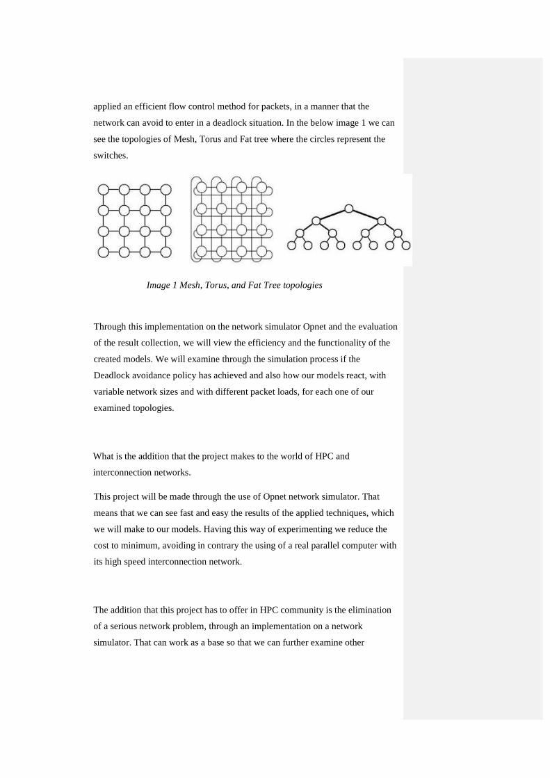
network can avoid to enter in a deadlock situation. In the below image 1 we can
see the topologies of Mesh, Torus and Fat tree where the circles represent the
switches.
Image 1 Mesh, Torus, and Fat Tree topologies
Through this implementation on the network simulator Opnet and the evaluation
of the result collection, we will view the efficiency and the functionality of the
created models. We will examine through the simulation process if the
Deadlock avoidance policy has achieved and also how our models react, with
variable network sizes and with different packet loads, for each one of our
examined topologies.
What is the addition that the project makes to the world of HPC and
interconnection networks.
This project will be made through the use of Opnet network simulator. That
means that we can see fast and easy the results of the applied techniques, which
we will make to our models. Having this way of experimenting we reduce the
cost to minimum, avoiding in contrary the using of a real parallel computer with
its high speed interconnection network.
The addition that this project has to offer in HPC community is the elimination
of a serious network problem, through an implementation on a network
simulator. That can work as a base so that we can further examine other

29
problems and techniques in high speed interconnection networks, and conclude
to a proper network architecture that can serve our purposes.
As a conclusion to the first chapter we can say that the need for HPC in our
times is very important so that we can give answers to important questions and
solve complex problems. Thus the complexity of a High Performance Computer
must be supported by an equal robust high speed network, problems that appear
on those machines and to the networks that support them are important to solve.
We need to pay attention on the details of such structures, like the network
switches or the interconnection lines that support our systems, depending
always on the different purposes and use for which we need such machines.


31
2 State of the art
In this 2nd chapter we will situate the position of our problem explaining the
related areas of interest for our work. We will refer to the proposed actions that
exist and can handle deadlock, focusing specially on the deadlock avoidance
concept and its possible solutions. In the final section we are going to refer the
relative with our project previous works that have studied the deadlock problem
and its solution through the use of the virtual channels.
2.1 In which level is situated our problem
The HPC area is a rapidly evolving area of investigation which attends to help
on the solution of complex problems. To succeed this purpose High
Performance Computing has to make use of a combination of sophisticated
hardware computing infrastructures with high speed interconnection networks.
The hardware or network infrastructures may vary depending on the needs of
the HPC designer. HPC hardware structures making use of parallel
programming techniques to solve the complex problems, techniques that need
continuous and high speed data exchange between the computational nodes. As
the complexity of a problem increases and the programming technique acquire
more data exchange to achieve the solution of the problem, the interconnection
network is some times unable to handle all this amount of data due to finite
hardware resources.
The interconnections networks are used nowadays for several applications and
for different purposes. The type of the interconnection network varies
depending on the goal that we want to achieve or the system architecture that is
going to be applied. Different types of networks are listed below.
� Backplane buses and system networks
� Processor to memory interconnections
� Internal networks for asynchronous transfer mode (ATM)
� Multicomputer networks

� High Performance Computing interconnection networks
� Distributed shared-memory multiprocessor interconnection
� LAN's, MAN's, WAN's
� Industrial application networks
In our case we will focus on the interconnection network of High Performance
Computers. Thus the demand for bigger computation power is always
increasing, it create needs for the reliability and the accuracy of the
interconnection network. The communication between processors in a
computational node of an HPC system is done through buses. These
connections have small length which is limited in the length of few millimeters
and due to their construction materials can provide small communication
latency. This latency compared with the communication latency on an
interconnection network is almost zero, thus the length of a communication line
can exceed in some meters or tens of meters and the constructional material of
the communication wire can cause extra latency to the packet delivery. Having
in mind that the network is the slowest form of communication between
processors, we would like to make the communication time as smaller as
possible and eliminate communication problems. The network has to support
respectively the transition of the information, without causing delays or
rejection of packets, due to several problems that can appear.
For the design of the interconnection network we have to consider the network
infrastructure that will form the network and will connect the nodes between
them. The type of communication wires, the switches or routers and their
combination with the routing techniques that we need, have to be examined in
detail so that we can have a robust interconnection network and avoid the
problems that can appear under a heavy communication load.
To understand the causes of an interconnection problem, we have to focus on
the way that the intermediate hardware infrastructures, that our network uses,
work. The switches on an interconnection network play a serious role in the
transition of packet from their source to their destinations, thus they manage and
33
provide a path for the traversed packet. In the case that a problem occurs or the
heavy load makes these infrastructures unable to serve the network, we need to
focus our interest on the internal architecture of a switch and examine the
pipeline with which it functions. We need to study the different elements from
which a switch is structured, how they are combined together to work and what
are the necessary alterations that we need to make in hardware and logic level to
solve a network problem.
For the purposes of the deadlock avoidance with the use of virtual channels is
necessary to examine in this lower level, how the packets enter and make use of
the switch hardware resources, how the problems appear while the traffic load
increases and what are the possible changes that need to be made in hardware
and software level, to eliminate the possibility that a deadlock will occur.
While the amount of traffic load increases, increase also and the possibility of
simultaneous need by the packets to have access over the same hardware
resources, such as the input and output buffers of the switch. Because of that we
have to use a technique such as virtual channels that can provide alternative
ways of access on these resources and will not stop or delay significantly the
packet traversal on the network.
For the investigation of such a problem, we will need a tool that can provide us
access to the various levels of the network structure, allowing us to alter the
internal logic and components of our network elements. Proper tool for that
purpose can be a network simulator that will support changes in that level and
can give us results, through which we can examine the effects of our alterations
and if needed improve the structural logic.
2.2 What are the existing proposals for the problem
As the big delays on the packets transition can significantly reduce the
calculation ability of an HPC structure, the undelivered packets can have
catastrophic sequences for the ability of such a machine to produce the correct
amount of work, due to lack of information exchange. Some of the most serious
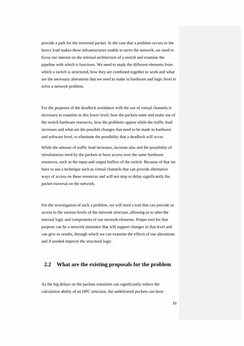
problems that can cause undelivered packets inside our network are listed below
in image 2 with their proposed solutions.
Phenomena like deadlock, livelock or starvation, appear in interconnection
networks due to the finite number of resources and can create the problem of
undelivered packets or even paralyze the network. This is caused because of
conflicts between agents and resources, in our case packets and packet buffers.
An explanation for each one of the phenomena follows.
Deadlock
Deadlock is the situation where two or more competing agents waiting each one
for the other to release critical resources. The problem occurs because none of
the agents is able to progress due to the denial of another agent to release its
resources or to reach in a compromise.
Livelock
Livelock is the condition when two or more agents are continually changing
their state in response with the state of other agents, causing a continuous loop.
Image 2 Causes of undelivered packets

35
Result of that is that none of the agents can have access to the resources.
Livelock is similar with deadlock thus no progress is made over the resources,
and differs in the way that none of the agents is blocked or waiting for a
resource.
Starvation
Starvation is the situation that the competing agents may never be granted to the
requested resources falling in the situation that an agent is starved. A network
falls in starvation when the requests by the agents for resources are coming
more frequently that they can been handled.
For our case, we will examine the deadlock phenomenon, which is the most
serious of all the above. Deadlock may occur due to four conditions which are
the Mutual exclusion, the Hold and Wait condition, a no pre-emption condition
or due to circular wait condition. A small explanation for each one of them
follows.
3 Mutual exclusion condition is when a resource is either assigned to one agent
or it is available.
4 Hold and wait condition is when an agent which already holding resources
may request new resources.
5 Non preemption condition is when only an agent who holds a resource may
release it
6 Circular wait condition is the condition where two or more agents form a
circular chain where each agent waits for a resource that the next agent in the
chain holds.
For Deadlock there are three known solution techniques, Prevention, Recovery
and Avoidance. Each one of them refers to a different approach for the
deadlock.
Prevention
The system itself is built in such a way that there are no deadlocks. That means
that the system makes sure, that at least one of the necessary for deadlock
conditions will never occur. This is done for example in circuit switching where
the resources are granted before the transmission starts. It is very conservative
approach and may lead to very low resource utilization.
Recovery
Deadlock recovery does not impose any restrictions to the routing mechanism,
but rather allows deadlock to occur. Deadlock recovery attends to give a
solution to the problem after that has caused, forcing the agents that hold
resources to release them, allowing with that way other agents to use those
resources and break the deadlock.
Avoidance
Deadlock avoidance is the technique where certain information about agents is
available in advance of resource allocation. For every resource request, the
system sees if granting the request will mean that the system will enter an
unsafe state, meaning a state that could result in deadlock. The system then only
grants request that will lead to safe states. In order for the system to be able to
figure out whether the next state will be safe or unsafe, it must know in advance
at any time the number and type of all resources in existence, available, and
requested. One known algorithm that is used for deadlock avoidance is the
Banker's algorithm. However, for many systems it is impossible to know in
advance what every process will request. This means that deadlock avoidance is
often impossible.
In our project we will focus specially on the deadlock avoidance technique and
how this is achieved with the use of virtual channels. The virtual channels will
provide to our system extra alternative resources that can be used by the agents,
meaning packets, to avoid other blocked resources and with that way avoid

37
deadlock. Changes in the mechanism of the switch have to be done so that can
support this new structure and avoid resource dependencies to occur. The logic
of the mechanism now has to put a specific order on the resources and
restrictions on the way that these resources are going to be accessed by the
packets. The implementation and the examination of that proposal will be
studied through the network simulator in which we will implement and test our
models.
2.3 Related works
Previous implementations for the deadlock refer to the solution of the problem
in different levels and with various ways. Deadlock problem appears from
processor to processor communications, to different types of networks, deadlock
on chip level or most often in databases and multi-threaded applications.
Deadlock occurs in software where a shared resource is locked by one thread
and another thread is waiting to access it and something occurs so that the thread
holding the locked item is waiting for the other thread to execute. Another case
where deadlock can occur is in databases where one application has asked for a
lock on a table. It then requires a second table but another application has locked
the second table and is waiting to get a lock on the first.
Some of the related with our project implementation refer to various approaches
like the use of adaptive routing using only one virtual channel [4], virtual lanes
for ATM networks [5] or the implementation on QNOC router with a dynamic
virtual channel allocation [6]. In these researches is studied the effect and the
utilization of the virtual channels and the appropriate number of them for the
deadlock solution but with different types of network or routing strategy.
None of the previous implementations or approaches to the problem is referring
to the solution of deadlock avoidance through a simulation process, for the
specific network models that we are going to study, and the comparison of the

results between these tree topologies. In our case, thus the construction of a
network with the appropriate policy needs further examination and
implementation we are using a network simulator. This approach offers the
ability to change the numbers of virtual channels and the buffer capacity that
each one of they contains. Also we can experiment with the deadlock avoidance
policy and see how we can implement it to our network topologies, with the
minimum cost on resources while having the desired result.

39
3 Theoretical backs
In the 3rd chapter we will focus on the problem of deadlock and its possible
solutions. We will see the reasons that cause the deadlock and how we can avoid
it by the use of virtual channels. The definition of virtual channels will be given
next and the possible uses that the virtual channels have. At the last part of the
chapter will be described the parts of the Opnet network simulator that our
implementation is going to uses and important details about their use and
functionality.
3.1 Theory
3.1.1 Deadlock Avoidance
A deadlock is a situation where in two or more competing actions are waiting
for the other to finish, and thus neither ever does. It is often seen in a paradox
like 'the chicken or the egg'.
In computer science, deadlock refers to a specific condition when two or more
processes are each waiting for each other to release a resource, or more than two
processes are waiting for resources in a circular chain. Deadlock is a common
problem in multiprocessing where many processes share a specific type of
mutually exclusive resources known as a software, or soft, lock.
Image 3 Deadlocked configuration
Deadlock occurs in an interconnection network when a group of agents,
usually packets are unable to make progress because they are waiting on one
another to release resources, usually buffers on channels. If a sequence of
waiting agents forms a cycle, as it shown in image 3, then the network is
deadlocked. This can have catastrophic sequences for the network. When some
resources of the network are been occupied with deadlocked packets other
packets that coming block on these resources and cannot proceed to their
destination. [1 ch.14]
For Deadlock handling there are three known techniques that has been used
and these are
1. Deadlock Prevention,
2. Deadlock Avoidance
3. Deadlock Recovery
To prevent this situation, networks must either use deadlock avoidance, method
that guarantee that a network cannot deadlock, or deadlock recovery in which
deadlock is detected and corrected. As in almost all the modern networks [1
ch.14], our project will make use of the Deadlock Avoidance technique.
Deadlock appears because the network resources such as channels and buffers
are limited. We have to focus that in the switched based networks, like these we
are going to study, where each switch is connected with a processor. The
switches that are connected with a processor can send and receive messages
from the processor.. Due to the similarity between the direct networks and the
switch based networks we can apply that policy for the deadlock avoidance. [3
ch.1]
41
To achieve the Deadlock Avoidance, the routing mechanism applied has to
restrict the allowed paths for the packets that keep deadlock free the global
network state. An approach for the solution of this is to put an order on the
resources that want to be accessed by the packets, in the minimum way for
having network full access. Assigning the resources partially or totally to the
packets, so that cannot exist the possibility that a circular dependency will
appear. With that way we are applying escape paths to the packets, no matter
where they are inside the network, avoiding the probability that they will come
in a deadlock situation.
Critical resources on the deadlock avoidance, in network level, are the
connection lines and the buffers associated with them. There must be an order
in the access of the resources by the packet, while these are travelling from their
source to the destination.
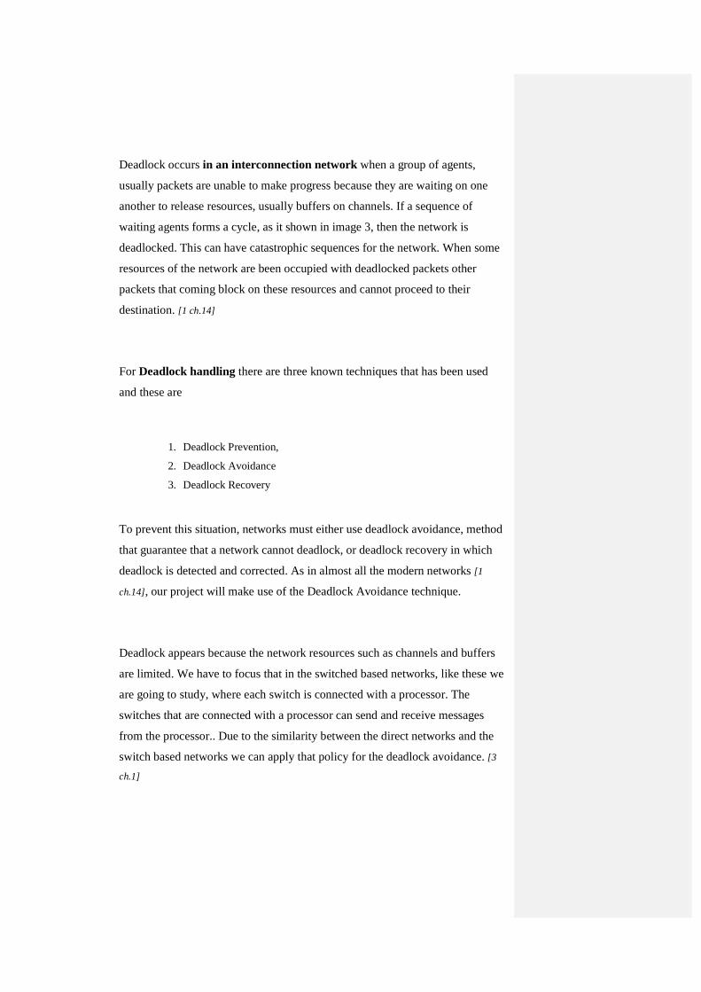
When a packet inserted in the network at the phase 0 is entering in a switch.
Through the communication lines goes to the phase 1 where the next switch is,
and continues until it reach its destination. While not exist recirculation of
packets, once a packet have reserved an output channels from the first phase, it
cannot request any other output channel from the same phase, thus there are no
dependencies between the output channels of the same phase. Similarly a packet
that has reserved an output channel on a given phase, cannot request for an
output channel at a previous phase. With that way we only have dependencies
Image 4 Stages of traversing packet
from this phase to the next phase. Sequence of that is that we don't have cyclic
dependency between channels and we avoid deadlock.
While using a flow control method, like store and forward or virtual cut
through, the agents are packets and the resources are the packet buffers. At any
given time each packet can only occupy one packet buffer. When a packet
request for a new packet buffer, it should release the old packet buffer a short
time later. In our case the resources will be the virtual channels that will replace
the packet buffers as entities.
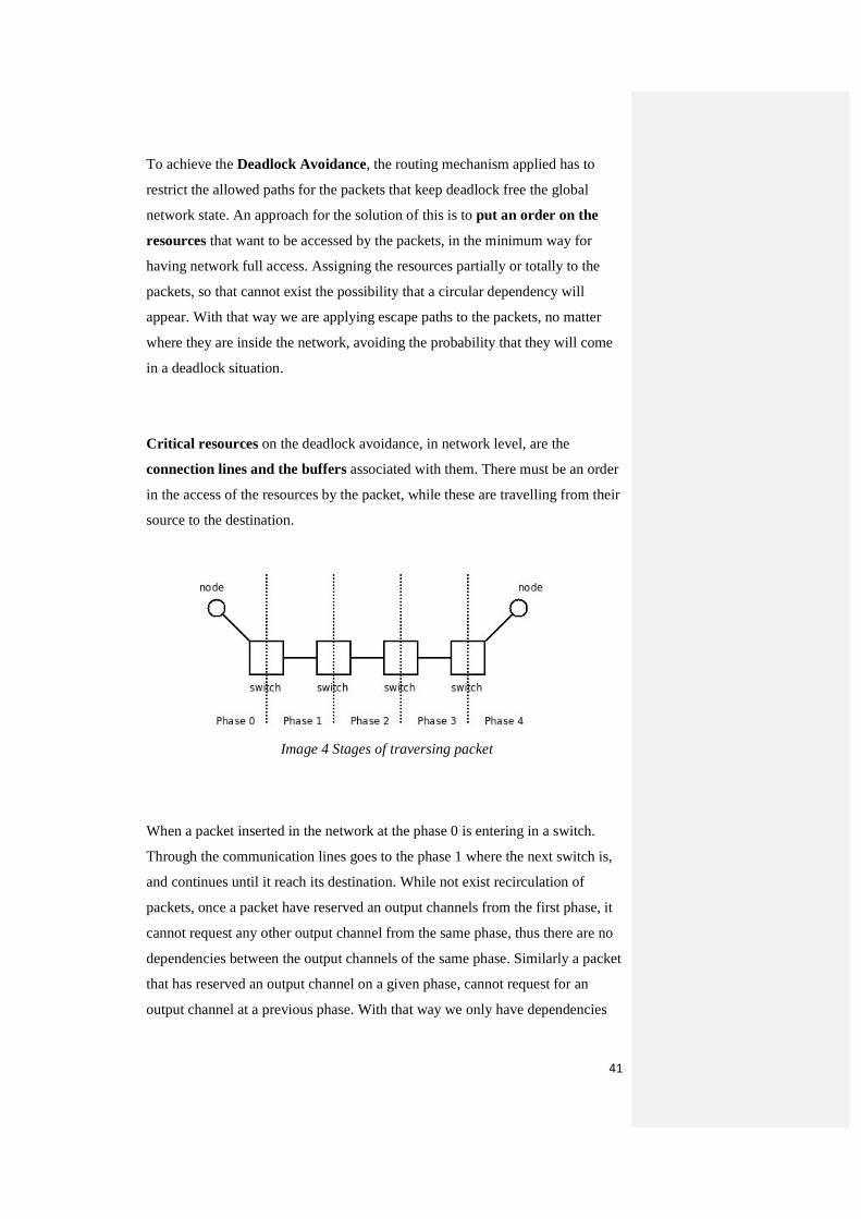
The lines (agents) and the virtual channels (resources) are related with “Wait
for” and “Hold” relations. If a line holds a buffer, then that buffer is waiting
from the line to be released. If that not happen, a deadlock occur.
Image 6 Wait for and Hold graph
A representation of the relations between agents and resources can be done
through the dependence graph and the wait-for graph . In both above images 5
an 6, we can see how connections A and B occupying some resources while
they are waiting for some others. A occupies channels u and v and waits for
channel w which is occupied by the connection B. Similarly the connection B
holds channels w and x and waits for channel u.
If we focus on the Hold relations that lead to the buffers u and w from the lines
A and B in Image 6.a, and we redraw these lines to the opposite direction as
Image 5 Dependence graph
43
Wait for relations we have the Image 6.b. Here we can see, from the dotted
arrows that appear a circulation between the resources. This circulation shows
us that the configuration is deadlocked.
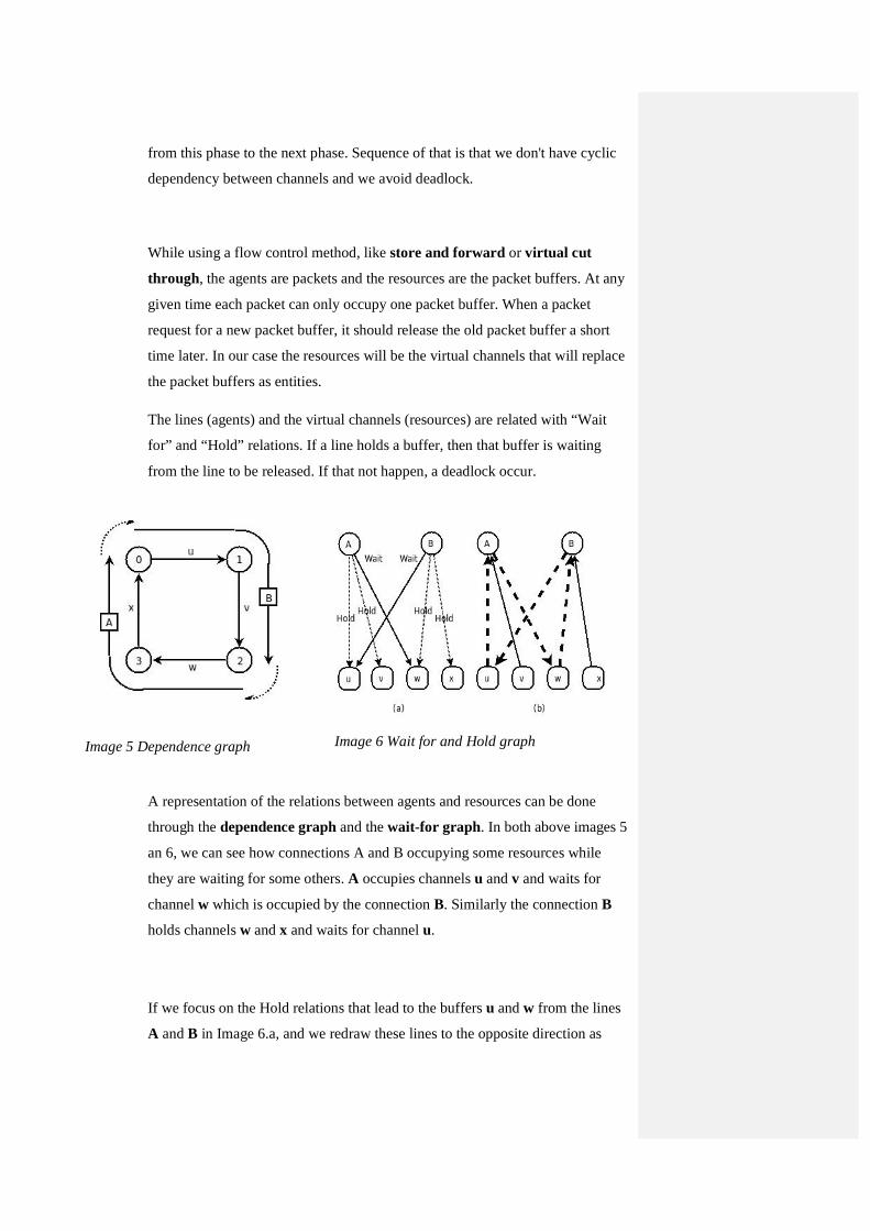
In order to occur deadlock, the lines have to acquire buffer resources and wait
on others, with a way that creates a cycle in the wait for graph. This cycle is a
necessary nut not sufficient condition for a deadlock. If we can manage to
eliminate the cycles from the resource dependence graph we can we eliminate
the possibility of a circular dependence on the wait for graph and as a sequence
we avoid to deadlock the network.
If the above scheme we replace the buffer resources with the two equal virtual
channels (explained in next section), we will have a dependence graph like the
one below, in Image 7.
Image 7 Dependence graph with 2 VC
3.1.2 Virtual Channels
To avoid Deadlock to our network we have to apply a flow control method to
allocate the appropriate for the packet resources. Important resources for the
interconnection network are the communications lines and the buffers. Buffers
are storage inside nodes and switches, with the form of a memory. In this
memory is where the packets are temporarily stored, while traversing to their
destination through the communication lines. Dependent on the switching
technique and flow control that we use, we may respect to the packets either as
entire packets or as flits. Flits or flow control units, are the smaller units from
which the packet consists and create the header, data and tail sections of the
packet. The flits are also divided in smaller units called phits (phase digits)
which are the binary representation of a flit.
While the topology of the network determines the possible ways that a packet
has to reach its destination, the flow control is the method applied to the
network that organizes the network traffic. Flow control determines when and
how a travelling packet inside the network can overcome network problems and
advance itself until destination. This applied strategy must avoid resource
conflicts between packets, keeping with that way the channels idle.
As an analogy to the real world, we should provide alternative pathways if it
occurs a problem in a highway road, so that the incoming traffic can overcome
the accident and continue its way. Having this analogy in mind, at hardware
level, if a packet gets blocked in a buffer while expecting other resources to get
free, incoming packets should not get blocked by this packet. The flow control
mechanism should provide them an escape path in the form of an alternative
buffer, so that the packet can proceed. The implementation of this in hardware is
the partition of the used buffer in several pieces that we call virtual channels.
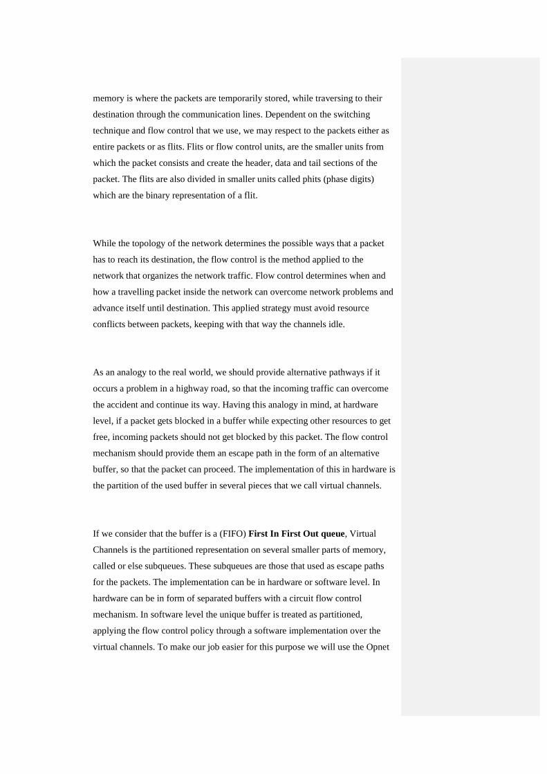
If we consider that the buffer is a (FIFO) First In First Out queue, Virtual
Channels is the partitioned representation on several smaller parts of memory,
called or else subqueues. These subqueues are those that used as escape paths
for the packets. The implementation can be in hardware or software level. In
hardware can be in form of separated buffers with a circuit flow control
mechanism. In software level the unique buffer is treated as partitioned,
applying the flow control policy through a software implementation over the
virtual channels. To make our job easier for this purpose we will use the Opnet
45
network simulator, partitioning virtually a predefined model of a FIFO buffer
queue as it shown below on image 8.
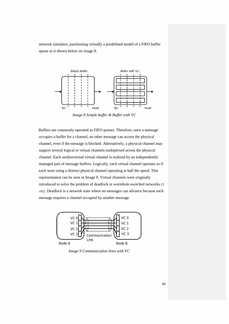
Buffers are commonly operated as FIFO queues. Therefore, once a message
occupies a buffer for a channel, no other message can access the physical
channel, even if the message is blocked. Alternatively, a physical channel may
support several logical or virtual channels multiplexed across the physical
channel. Each unidirectional virtual channel is realized by an independently
managed pair of message buffers. Logically, each virtual channel operates as if
each were using a distinct physical channel operating at half the speed. This
representation can be seen in Image 9. Virtual channels were originally
introduced to solve the problem of deadlock in wormhole-switched networks [3
ch2]. Deadlock is a network state where no messages can advance because each
message requires a channel occupied by another message.
Image 8 Simple buffer & Buffer with VC
Image 9 Communication lines with VC
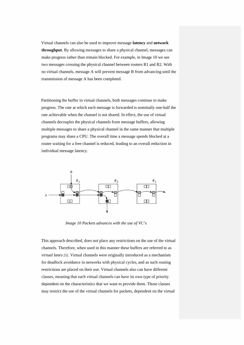
Virtual channels can also be used to improve message latency and network
throughput . By allowing messages to share a physical channel, messages can
make progress rather than remain blocked. For example, in Image 10 we see
two messages crossing the physical channel between routers R1 and R2. With
no virtual channels, message A will prevent message B from advancing until the
transmission of message A has been completed.
Partitioning the buffer in virtual channels, both messages continue to make
progress. The rate at which each message is forwarded is nominally one-half the
rate achievable when the channel is not shared. In effect, the use of virtual
channels decouples the physical channels from message buffers, allowing
multiple messages to share a physical channel in the same manner that multiple
programs may share a CPU. The overall time a message spends blocked at a
router waiting for a free channel is reduced, leading to an overall reduction in
individual message latency.
This approach described, does not place any restrictions on the use of the virtual
channels. Therefore, when used in this manner these buffers are referred to as
virtual lanes [5] . Virtual channels were originally introduced as a mechanism
for deadlock avoidance in networks with physical cycles, and as such routing
restrictions are placed on their use. Virtual channels also can have different
classes, meaning that each virtual channels can have its own type of priority
dependent on the characteristics that we want to provide them. Those classes
may restrict the use of the virtual channels for packets, dependent on the virtual
Image 10 Packets advances with the use of VC’s
47
channel buffer utilization or the priority type of a packet. For example, packets
may be prohibited from being transferred between certain classes of virtual
channels to prevent cyclic waiting dependencies for buffer space. Thus, in
general we have virtual channels that may in turn be made of multiple lanes.
While the choice of virtual channels at a router may be restricted, it does not
matter which lane within a virtual channel is used by a message, although all of
the flits within a message will use the same lane within a channel.
Acknowledgment traffic is necessary to regulate the flow of data and to ensure
the availability of buffer space on the receiver. Acknowledgments are necessary
for each virtual channel or lane, increasing the volume of such traffic across the
physical channel. Furthermore, for a fixed amount of buffer space within a
router, the size of each virtual channel or lane buffer is now smaller. Therefore,
the effect of optimizations such as the use of acknowledgments for a block of
flits or phits is limited. If physical channel bandwidth is allocated in a demand-
driven fashion, the operation of the physical channel now includes the
transmission of the virtual channel address to correctly identify the receiving
virtual channel, or to indicate which virtual channel has available message
buffers.
For the recognition of the packets and their corresponding direction to the
virtual channels, has to be added a flit more to the header of each packet. That
flit is inserted in the source node and will contain the number with the desired
virtual channel for the packet. With that way, it will be described the preferred
route that the packet will follow through the network, and will be applied the
necessary flow control mechanism on the input or output virtual channels of a
switch.
3.1.3 OPNET
For our project, the implementation will be based on the Opnet network
simulator. Opnet network simulator is a simulation tool equipped with many
predefined models of nodes, servers, switches and communication lines, which

exist in the market. Also supports a wide range of protocols, and allows altering
on the predefined characteristic models. The simulator allows user intervention
in 4 different levels that start from the network or subnetwork level, to the
module level, the process level and in the lower part is the code level. Here
Opnet network simulator supports the use of external commands based in the
programming language of C/C++.With that we way we can manage the existing
models and protocols, or design and create a new one for our purposes.
3.1.3.1 Network
The network defines the overall scope of the system we are going to simulate.
It’s a representation of the objects that participate in the network construction.
The network model specifies the objects inside the network, as well as their
physical locations, interconnections and configurations. It can contain
subnetworks and nodes, connected through several links, giving a more complex
structure to the network. This supported complexity provides us easiness to
design networks similar to the appearance and functions, with the real ones that
we want to simulate.
The interprocessor communications as in High Performance Computing can be
viewed as a hierarchy of services. These services begin form a higher level, the
application layer, in which are performed actions for the preparation of the
packets and the data encryption and data compression, until the physical layer
which is responsible for the transition of the packets that come from a higher
layer. We can view such a layering in the communications services, especially
for the Local and Wide Area Networks (LAN's and WAN's). This layering can
be characterized in three layers, and these are from the lower to the higher.
Physical layer
The physical layer is responsible for packet transfer through the physical
channel from switch to switch.

49
Switching layer
Switching layer make use of the physical layer, implementing mechanisms so
that can forward the messages to their destination.
Routing layer
At the routing layer are taken the routing decisions for the output channels that
can provide a path, so that the packet can continue through the network to its
destination.
The routing mechanisms and their properties (deadlock or livelock freedom) are
determined mostly by the switching layer. The switching techniques that are
implemented inside the switching layer are responsible to set the switch inputs
and outputs and the appropriate time that the packet needs to travel the path
inside the switch. [3 ch.3]
These switching techniques make use of flow control mechanisms that are
responsible for the packet transfer synchronization between the switches. The
flow control mechanisms are related with the management of the packet buffers.
Determine how the buffers are accessed and released by the packets and which
is the appropriate policy when exist blocked packets inside these buffers. [3 ch3]
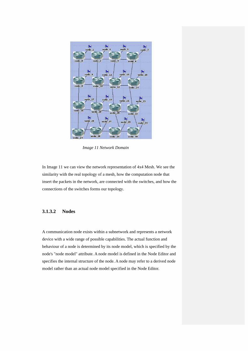
Image 11 Network Domain
In Image 11 we can view the network representation of 4x4 Mesh. We see the
similarity with the real topology of a mesh, how the computation node that
insert the packets in the network, are connected with the switches, and how the
connections of the switches forms our topology.
3.1.3.2 Nodes
A communication node exists within a subnetwork and represents a network
device with a wide range of possible capabilities. The actual function and
behaviour of a node is determined by its node model, which is specified by the
node's "node model" attribute. A node model is defined in the Node Editor and
specifies the internal structure of the node. A node may refer to a derived node
model rather than an actual node model specified in the Node Editor.

51
Switch node model
The Switch node model supports large numbers of incoming and outgoing data
links and performs packet routing at high speeds. Within the model are defined
the characteristics that we want to provide, in form of a sequence of modules
Computation node model
Can generate and receive transfers of files or sparse packets, also depend on the
architecture and the functionality that we want to apply to our network.
Communication lines
Links allow communication of information between nodes in the form of
structured messages called packets. When a packet is submitted to a transmitter
in a source node, the packet is conveyed over a link to a receiver in a destination
node. A transmitter may support multiple outgoing channels into a link and,
similarly, a receiver may support multiple incoming channels from a link as it
shown below in the image 12.
Image 12 Communication channels

A link is actually composed of one or more communication channels, each of
which defines a connection between a transmitter channel and a receiver
channel. A communication channel can be thought of as a pipe, where packets
are placed in one end by a transmitter channel and retrieved at the other end by a
receiver channel. If a link has multiple communication channels, it can be
thought of as a "bundle" of pipes, each one conveying packets from the source
node to the destination node.
Simplex and Duplex Point-to-Point Links
A point-to-point link can be thought of as a bundle of one or more
communication channels between the transmitter(s) and receiver(s) that it
connects. Within a point-to-point link, the number of communication channels is
static, because there is one communication channel between each transmitter
channel and receiver channel of the same index. Packets sent by transmitter
channel in the source node will be received by the receiver channel with same
index in the destination node. Each communication channel acts independently
of the others in the same link, as though it were defined in a separate and
parallel point-to-point link.
A simplex point-to-point link defines a connection from a transmitter in the
source node to a receiver in the destination node. Packets are conveyed in that
one direction. A duplex point-to-point link, however, defines a pair of
connections between two nodes, connecting a transmitter in each node to a
receiver in the other. Packets can flow in both directions, from each node to the
other.
For a point-to-point link to be operable, it must be attached to point-to-point
transmitters and receivers in the nodes that it connects. The transmitter and
receiver of a simplex point-to-point link are designated using its "transmitter"
and "receiver" object attributes. For duplex links, four attributes ("transmitter a",
"receiver a", "transmitter b", and "receiver b") serve to identify the modules
within the nodes to which the link is attached.
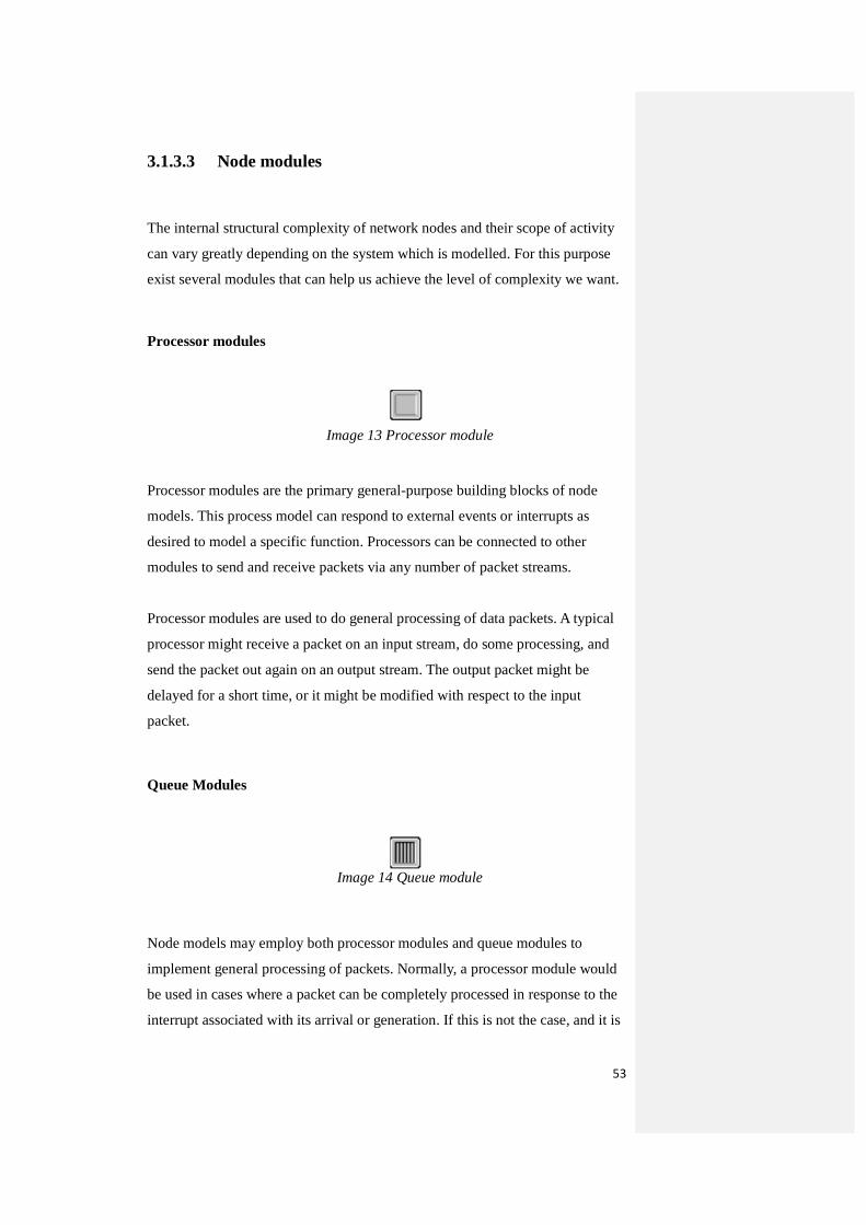
53
3.1.3.3 Node modules
The internal structural complexity of network nodes and their scope of activity
can vary greatly depending on the system which is modelled. For this purpose
exist several modules that can help us achieve the level of complexity we want.
Processor modules
Processor modules are the primary general-purpose building blocks of node
models. This process model can respond to external events or interrupts as
desired to model a specific function. Processors can be connected to other
modules to send and receive packets via any number of packet streams.
Processor modules are used to do general processing of data packets. A typical
processor might receive a packet on an input stream, do some processing, and
send the packet out again on an output stream. The output packet might be
delayed for a short time, or it might be modified with respect to the input
packet.
Queue Modules
Node models may employ both processor modules and queue modules to
implement general processing of packets. Normally, a processor module would
be used in cases where a packet can be completely processed in response to the
interrupt associated with its arrival or generation. If this is not the case, and it is
Image 13 Processor module
Image 14 Queue module
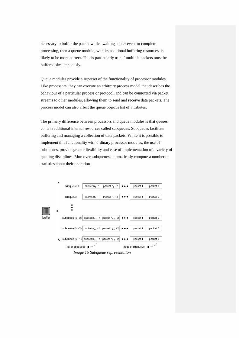
necessary to buffer the packet while awaiting a later event to complete
processing, then a queue module, with its additional buffering resources, is
likely to be more correct. This is particularly true if multiple packets must be
buffered simultaneously.
Queue modules provide a superset of the functionality of processor modules.
Like processors, they can execute an arbitrary process model that describes the
behaviour of a particular process or protocol, and can be connected via packet
streams to other modules, allowing them to send and receive data packets. The
process model can also affect the queue object's list of attributes.
The primary difference between processors and queue modules is that queues
contain additional internal resources called subqueues. Subqueues facilitate
buffering and managing a collection of data packets. While it is possible to
implement this functionality with ordinary processor modules, the use of
subqueues, provide greater flexibility and ease of implementation of a variety of
queuing disciplines. Moreover, subqueues automatically compute a number of
statistics about their operation
Image 15 Subqueue representation
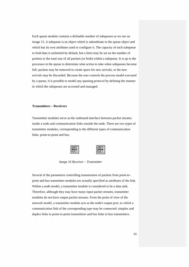
55
Each queue module contains a definable number of subqueues as we see on
image 15. A subqueue is an object which is subordinate to the queue object and
which has its own attributes used to configure it. The capacity of each subqueue
to hold data is unlimited by default, but a limit may be set on the number of
packets or the total size of all packets (or both) within a subqueue. It is up to the
processes in the queue to determine what action to take when subqueues become
full: packets may be removed to create space for new arrivals, or the new
arrivals may be discarded. Because the user controls the process model executed
by a queue, it is possible to model any queuing protocol by defining the manner
in which the subqueues are accessed and managed.
Transmitters – Receivers
Transmitter modules serve as the outbound interface between packet streams
inside a node and communication links outside the node. There are two types of
transmitter modules, corresponding to the different types of communication
links: point-to-point and bus.
Image 16 Receiver – Transmitter
Several of the parameters controlling transmission of packets from point-to-
point and bus transmitter modules are actually specified as attributes of the link.
Within a node model, a transmitter module is considered to be a data sink.
Therefore, although they may have many input packet streams, transmitter
modules do not have output packet streams. From the point of view of the
network model, a transmitter module acts as the node's output port, to which a
communication link of the corresponding type may be connected: simplex and
duplex links to point-to-point transmitters and bus links to bus transmitters.

3.1.3.4 Connections
Packet streams
Packet streams are connections that carry data packets from a source module to
a destination module. They represent the flow of data across the hardware and
software interfaces within a communication node. There are three different
methods for transferring a packet over a stream and notifying the destination
module of its arrival: scheduled, forced, or quiet.
Statistic wires
Statistic wires carry data from a source module to a destination module. Unlike
packet streams, which convey packets, statistic wires convey individual values.
They are generally used as an interface by which the source module can share
certain values with the destination module, and thereby provide information
regarding its state. Each module within a node has a set of local output statistics
whose values are updated at correct times during the simulation. It is this set of
statistics that can act as the sources of statistic wires.
Image 17 Packet stream
Image 18 Statistic stream
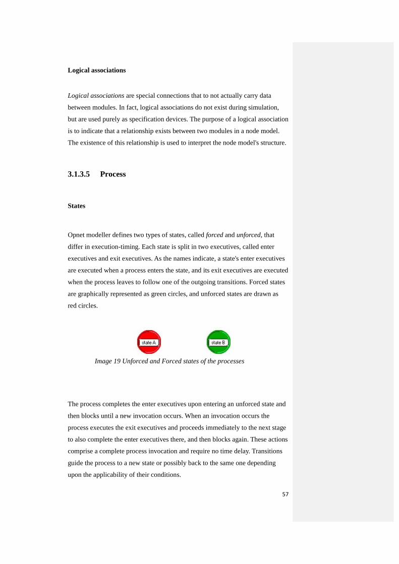
57
Logical associations
Logical associations are special connections that to not actually carry data
between modules. In fact, logical associations do not exist during simulation,
but are used purely as specification devices. The purpose of a logical association
is to indicate that a relationship exists between two modules in a node model.
The existence of this relationship is used to interpret the node model's structure.
3.1.3.5 Process
States
Opnet modeller defines two types of states, called forced and unforced, that
differ in execution-timing. Each state is split in two executives, called enter
executives and exit executives. As the names indicate, a state's enter executives
are executed when a process enters the state, and its exit executives are executed
when the process leaves to follow one of the outgoing transitions. Forced states
are graphically represented as green circles, and unforced states are drawn as
red circles.
The process completes the enter executives upon entering an unforced state and
then blocks until a new invocation occurs. When an invocation occurs the
process executes the exit executives and proceeds immediately to the next stage
to also complete the enter executives there, and then blocks again. These actions
comprise a complete process invocation and require no time delay. Transitions
guide the process to a new state or possibly back to the same one depending
upon the applicability of their conditions.
Image 19 Unforced and Forced states of the processes

Unforced states allow a pause between the enter executives and exit executives,
and thus can model true states of a system. After a process has completed the
enter executives of an unforced state, it blocks and returns control to the
previous context that invoked it.
Forced states are so called because they do not allow the process to wait. They
therefore cannot be used to represent modes of the system that persist for any
duration. In other words, the exit executives of a forced state are executed by a
process immediately upon completion of the enter executives. Therefore the exit
executives of a forced state are generally left blank, because they are equivalent
to the same statements placed at the end of the enter executives. Because forced
states cannot represent actual system states, they are not generally used as much
as unforced states. However they are useful in certain cases to graphically
separate actions or control flow decisions that are common to several unforced
states; graphically separating out definitions of decisions or actions this way can
sometimes provide better modularity of specification, as well a more visually
informative state transition diagram.
Transitions
Transitions describe the possible movement of a process from state to state and
the conditions under which such changes may take place. There are four
components to a transition's specification: a source state, a destination state, a
condition expression, and an executive expression. The specification may be
read as follows: when in the source state, if the condition is true, implement the
executive expression and transfer control to the destination state. The types of
the conditions are shown in image 20.

59
Non Empty Condition
A non empty condition is caused by an interrupt. If the interrupt value is true the
process goes from the source state to the destination state. If its needed, while
the non empty transitions is true, can execute a function before reach the
destination state. The condition and the executive expression are declared as
attributes of the transition.
Empty Condition
An empty condition simply transfers one state to an other, after the first stage
has completed its work on the exit executives. The empty condition does not
need an interrupt to occur to be enabled, and may have also as the non empty
condition an executive in its transfer between the source and destination states.
Transition to the same stage
A transition to the same stage is the loop action that Opnet provides, and may be
either a non empty condition or either an empty condition. This type of
transitions is used to have executive expressions that can be used for checks or
alternations on the used by the process variables.
Image 20 Transitions between states

3.1.3.6 Source code
Opnet modeller inside the process level uses code. This code is responsible for
all the actions we want to make in code level. With this code we can have
actions like receive and send packets, cause or receive interrupts, interface
control informations (ICI’s) and update statistics. These actions carry important
informations about the routing and switching mechanisms of our switch. Opnet
uses these integrated functions for all the basic uses like internal
communications inside module and communication between several modules.
The integrated code of Opnet supports the use of C/C++ with the use of the
internal compiler. This support gives us the opportunity to alter functionality in
even lower level of the constructed module and organize better our
programming structure.
In the 3rd chapter we have seen the theoretical base in which we are going to be
based for the analysis of our project. We have seen the definition of deadlock
and the reasons that cause the problem. Has been given the definition and the
usage of the virtual channels and has been explained the approach of the
deadlock avoidance with the use of virtual channels. Finally in the last section
we have seen the theoretical approach of the elements that we need to use on
our network simulator, Opnet, to implement the virtual channels.

61
4 Analysis
In this chapter we will focus on the theoretical part that encloses the solution of
the Deadlock avoidance policy with virtual channels, and how the theory has to
be used in practical level for our models. The analysis for the Deadlock
avoidance, has been based on the theory that has explained on chapter 3. Also
ideas about deadlock avoidance policy in different levels and memory
partioning for use as virtual channels have been collected from the books and
the papers of the bibliography. This analysis concentrates in the architecture of
existing models, specifically node and switch models that will explained fin the
start of the subject. These models are constructed in Opnet network simulator,
version 14.0.A, that the CAOS department is using, to examine various network
topologies, problems that appear in high performance networks and fault
tolerance. The pre-existing model is implemented by Diego Lugones, doctoral
student of the Department.
4.1 Previous model
The network model that has been used as base for out implementation was a
previous implementation of switches and nodes, through the Opnet simulator.
This implementation was an ATM switch based network structured in a 4x4
MESH topology with 16 switches and 16 compute node as shown in Image 21.
That means that the packets from their source to their destination are travelling
through the switches. Each one of the nodes is connected through a
communication line with a switch. Diagram of the Mesh topology is shown
below, where switches are indicated by “S” and compute nodes by “N”.

Image 21 4X4 MESH Topology
The nodes produce and send packets inside network with the use of the
switches. Each switch is reading information that exists in the header of the
packets and directs the packet to the necessary output port, so that it can
continue its trip inside network until its destination. We will focus in the
internal architecture of the models, the packets and the conditions that have to
exist inside the models, so that we can understand the logic with witch the
network functions. We will give special attention to the switch architecture that
is responsible for the deadlock and how we can avoid it implementing a routing
mechanism.
4.1.1 SWITCH
The theoretical model of the switch model in which we will be based, is an
input-output buffer switch. The michroarchitecture pipeline of the model is
show on the Image 22. The pipeline is separated in 5 stages. Stages 1 and 2 are
the input and output buffers that characterize our model. Stages 2, 3 and 4 are
the modules that create the central routing mechanism of the switch.
Respectively stage 2 is the routing mechanism, stage 3 is the arbitration and
finally stage 4 is the crossbar.
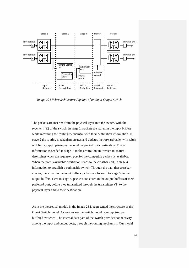
63
The packets are inserted from the physical layer into the switch, with the
receivers (R) of the switch. In stage 1, packets are stored in the input buffers
while informing the routing mechanism with their destination information. In
stage 2 the routing mechanism creates and updates the forward table, with witch
will find an appropriate port to send the packet to its destination. This is
information is sended in stage 3, in the arbitration unit which in its turn
determines when the requested port for the competing packets is available.
When the port is available arbitration sends to the crossbar unit, in stage 4
information to establish a path inside switch. Through the path that crossbar
creates, the stored in the input buffers packets are forward to stage 5, in the
output buffers. Here in stage 5, packets are stored in the output buffers of their
preferred port, before they transmitted through the transmitters (T) to the
physical layer and to their destination.
As in the theoretical model, in the Image 23 is represented the structure of the
Opnet Switch model. As we can see the switch model is an input-output
buffered switched. The internal data path of the switch provides connectivity
among the input and output ports, through the routing mechanism. Our model
Image 22 Michroarchitecture Pipeline of an Input-Output Switch
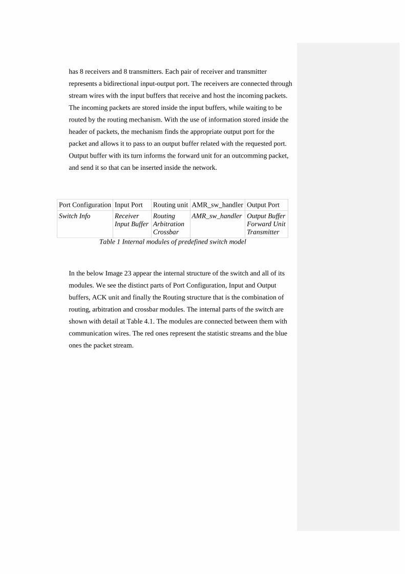
has 8 receivers and 8 transmitters. Each pair of receiver and transmitter
represents a bidirectional input-output port. The receivers are connected through
stream wires with the input buffers that receive and host the incoming packets.
The incoming packets are stored inside the input buffers, while waiting to be
routed by the routing mechanism. With the use of information stored inside the
header of packets, the mechanism finds the appropriate output port for the
packet and allows it to pass to an output buffer related with the requested port.
Output buffer with its turn informs the forward unit for an outcomming packet,
and send it so that can be inserted inside the network.
Port Configuration Input Port Routing unit AMR_sw_handler Output Port
Switch Info Receiver Input Buffer
Routing Arbitration Crossbar
AMR_sw_handler Output Buffer Forward Unit Transmitter
Table 1 Internal modules of predefined switch model
In the below Image 23 appear the internal structure of the switch and all of its
modules. We see the distinct parts of Port Configuration, Input and Output
buffers, ACK unit and finally the Routing structure that is the combination of
routing, arbitration and crossbar modules. The internal parts of the switch are
shown with detail at Table 4.1. The modules are connected between them with
communication wires. The red ones represent the statistic streams and the blue
ones the packet stream.
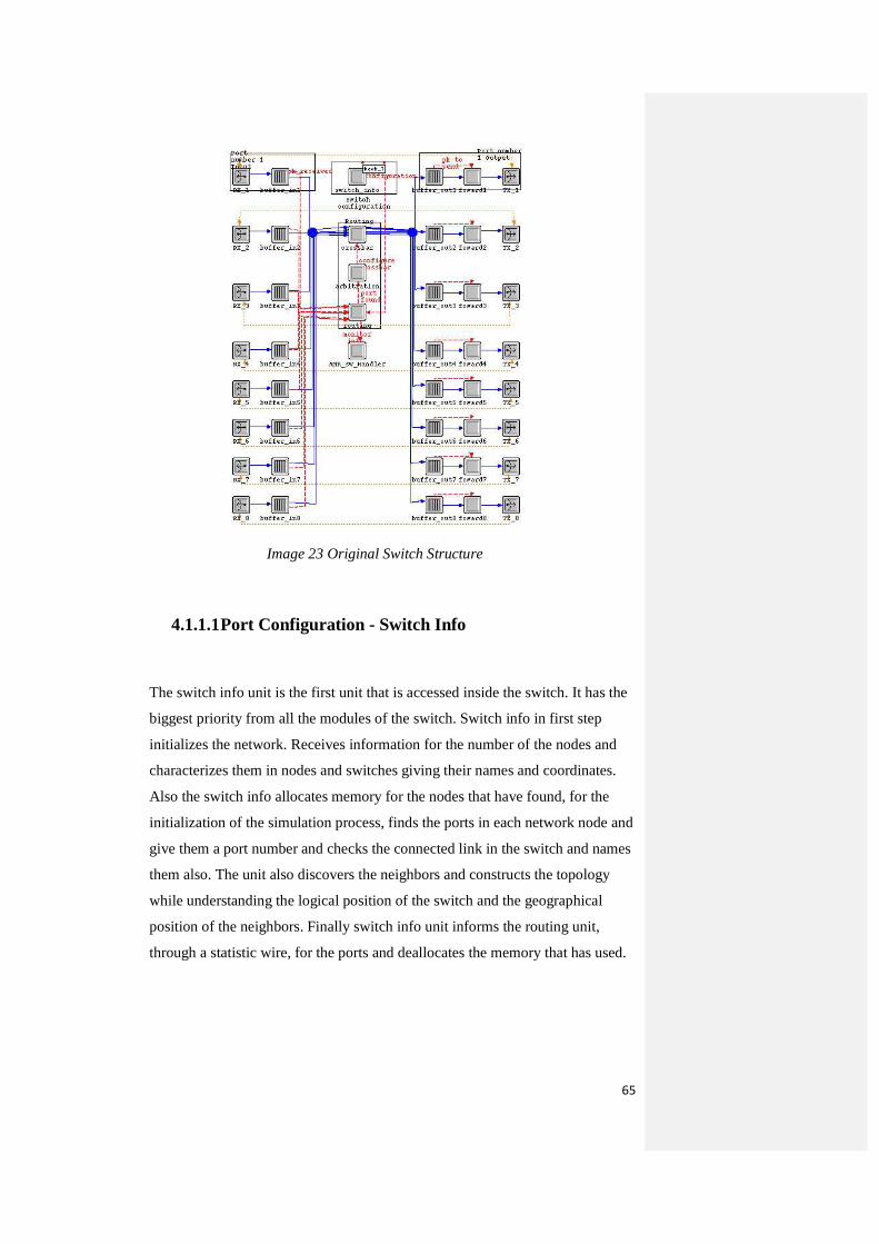
65
Image 23 Original Switch Structure
4.1.1.1 Port Configuration - Switch Info
The switch info unit is the first unit that is accessed inside the switch. It has the
biggest priority from all the modules of the switch. Switch info in first step
initializes the network. Receives information for the number of the nodes and
characterizes them in nodes and switches giving their names and coordinates.
Also the switch info allocates memory for the nodes that have found, for the
initialization of the simulation process, finds the ports in each network node and
give them a port number and checks the connected link in the switch and names
them also. The unit also discovers the neighbors and constructs the topology
while understanding the logical position of the switch and the geographical
position of the neighbors. Finally switch info unit informs the routing unit,
through a statistic wire, for the ports and deallocates the memory that has used.
4.1.1.2 Routing Logic
The central part of the switch which contains the routing logic is the
combination of 3 units. These units are the routing unit, the arbitration unit and
the crossbar. The functions that each units performs, so that the packets can find
an appropriate output port, are explained below.
Routing
Routing unit is the first step for the routing mechanism that the switch uses.
Routing unit is receiving information through statistic wires, firstly from the
switch info unit that informs the routing mechanism with information about the
switch situation. And from each one of the input buffers, that represent equal
input ports. Unit is also connected through statistic wires to send information,
with the AMR_sw_handler and with the arbitration unit.
The routing process starts by receiving the number of the input ports that is
connected with and allocating the appropriate memory space, for equal number
of packets that waiting to be routed. Then registers the statistics with which is
going to inform the Arbitration and AMR units. Here also initialized variable for
a Round robin approach to search between the input channels.
In the next state the routing unit receives from the switch info information,
through the statistic wire, in order to arbitrate. The information received is the
port configuration, with witch checks if the switch has a valid logical position,
the routing algorithm that is used for the packet traversal and the low and high
values of the threshold. In this part also the unit makes pair the input port
number with the equivalent input buffer.
Now the routing unit comes in a ”pause” situation, here waits to clean the
memory for waiting packets if simulation terminated, and also waits for
67
incoming interrupt by one of the connected input buffers. When an interrupt
occur the unit receives all the information from the interrupt, increases the
number of waiting packets by one and goes in the next state to route the packet.
The unit now searches in all ports, using round robin, to find a waiting packet
which needs to be routed. When it finds it, is applying the routing algorithm that
gives the appropriate output port, clearing the waiting packets memory for the
specified input and decreasing the number of the packets that waiting to be
routed by one. Before it exits from the state, make some checks for the received
output port, and sets that routing has completed, continuing with a self interrupt
proceeds to the next state.
Here the routing unit comes once more in a “pause” situation where it waits for
interrupt of a packet that waiting to be routed. If from the previous state is
declared that the routing has been done it proceeds to the next state where
prepares information to be sended in the Arbitration unit, informing that the
sender module has a packet in the queue.
Arbitration
The arbitration unit is a connection between the routing unit and the crossbar
unit. Arbitration receives information from the routing unit and passes it to the
crossbar. Given the input and the output port, the unit finds the correct stream to
forward the packet to that port.
Crossbar
Crossbar unit is responsible to receive incoming packets from the input buffers
and forward them to the requested output buffers that will lead them to a
predetermined output port. The Crossbar unit is informed from the Arbitration
unit by an interrupt, which declares that a specific input port has requested an
output port. The unit checks in the information received by the arbitration unit,

if its necessary update specific packet headers and forwards the packet to the
requested output port.
4.1.1.3 Input Port
The input port is characterized from two units. The receiver and the input
buffer. While the receiver accepts an incoming packet it forwards it to the
connected input buffer.
Receiver
Each receiver unit is representing the input port of the bidirectional channel.
The receiver is passing the incoming packet from the physical layer of the
channel to the input buffers of the switch.
Input Buffer
The input buffer is connected between the receiver unit, from where it receives
any incoming packet, with the routing unit which informs that a packet needs to
be routed and with the crossbar unit where its sends the packet so that can find
its requested output buffer and port.
Input buffer starts by initializing the statistic that will inform the routing unit,
receives the input port number and the internal bandwidth of the buffer. Before
exit the state declares that has no outcomming packet.
When the unit receives an interrupt for incoming packet, receive the packet and
sees if the buffer is empty. If it is, inserts the packet in the tail of the FIFO
queue, and informs the routing unit by a statistic wire that it has a packet
waiting to be routed, in the specified port.
69
When the module is having access to the interrupt that has appeared continues
to the next state. Now the module searches in the head of the queue, and if the
queue is not empty and contains a packet, module is having access to that
packet. The module next is getting the latency of the packet and update the
average occupation of the buffer, while removing the packet from the head of
the queue and receiving its size. In sequence the module send the packet through
a packet stream to the crossbar without causing an interrupt, thus earlier has
informed the routing mechanism through a statistic wire. The module computes
a delay based on the packet size, the internal bandwidth and delay of the switch
and when this time pass creates a self interrupt which makes the module
proceed to the last state.
In this last state the module checks for the buffer if its empty, to find if any new
packet has reached the head of the queue while the last packet was exiting from
the queue. If a new packet has appeared the module is getting once more access
to the head of the queue. Before it exits from the state takes the information
from the new arrived packet and informs once more the routing unit through a
statistic wire.
4.1.1.4 Output Port
Output Buffer
The output buffer module is connected with the crossbar unit from which
receives packets through a packet stream. The unit is also connected and
sending information, with the forward unit, through a statistic and a packet
stream.
Output buffer module, after initialize the necessary variables, proceeds to the
next state to receive a packet. Here the unit receives through an interrupt stream
the packet arrived. Checks if the tail of the queue is empty, and if it is, it inserts
the packet inside the tail. While there are no other packets that waiting to exit or
occupying the link, the unit informs the sender module that there is a packet
inside the queue.
In the next state, the unit receives a request to access the queue. If the queue is
not empty and contains packets, receive the first packet that is in the head of the
queue and calculates the buffer latency. After that removes the packet from the
queue, receiving its size and send it to the forward unit without causing an
interrupt because it has already informed the unit by a statistic wire. Thus the
packet will occupy the link for some time, the unit calculates that time based on
the bandwidth of the switch and the packet size. After that time expires the unit
causes a self interrupt that makes it proceed to the next state.
In this last state after the last packet has completely left from the queue, the unit
searches in the head of the packet once more if it has a new packet, and if it is
informs once more the forward unit through a statistic wire.
Transmitter
Each transmitter unit is representing the output port of the bidirectional channel.
The transmitter is passing the incoming packet from the output buffers to the
physical layer of the channel.
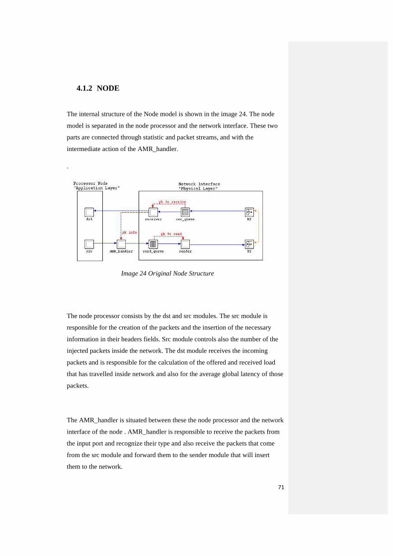
71
4.1.2 NODE
The internal structure of the Node model is shown in the image 24. The node
model is separated in the node processor and the network interface. These two
parts are connected through statistic and packet streams, and with the
intermediate action of the AMR_handler.
.
Image 24 Original Node Structure
The node processor consists by the dst and src modules. The src module is
responsible for the creation of the packets and the insertion of the necessary
information in their headers fields. Src module controls also the number of the
injected packets inside the network. The dst module receives the incoming
packets and is responsible for the calculation of the offered and received load
that has travelled inside network and also for the average global latency of those
packets.
The AMR_handler is situated between these the node processor and the network
interface of the node . AMR_handler is responsible to receive the packets from
the input port and recognize their type and also receive the packets that come
from the src module and forward them to the sender module that will insert
them to the network.
The network interface of the node is composed by six modules. These are the
transmitter (TX) and receiver (RX) units that give access to the physical layer,
the input and output buffers which are rec_queue and send_queue modules
respectively and the receiver and sender modules which are settled after the
buffers. When a packet is received by the network from the RX unit, is passing
into the rec_queue module tail, which works similarly with the switch buffers,
and informs through a statistic wire the receiver module that a packet is inside
the queue.
When the packet reach the head of the queue is sended through a packet stream
to the receiver module. The receiver module after a small time delay receives
the incoming packet and depended on the type of the packet, data or ack, gets
the latency values for each one of the packets. After that informs the
AMR_handler through a statistic wire and sends the packet to its destination, the
dst unit, through a packet stream. The same happens also, when a packet needs
to exit from the node. The packet is received by the send_queue and stored in
the tail of the queue. The send_queue informs the sender module with a statistic
and when the packet reaches the head of the queue is sended to the sender
module where after a small delay is sended to the physical layer.
4.2 Description of the proposition
Network Topologies
Starting from the network level, we will see how the network topologies are
structured, how a deadlock occurs and how a routing mechanism with the
support of virtual channels in the switch architecture can avoid the deadlock.
Beginning from that level will make easier the understanding of the problem
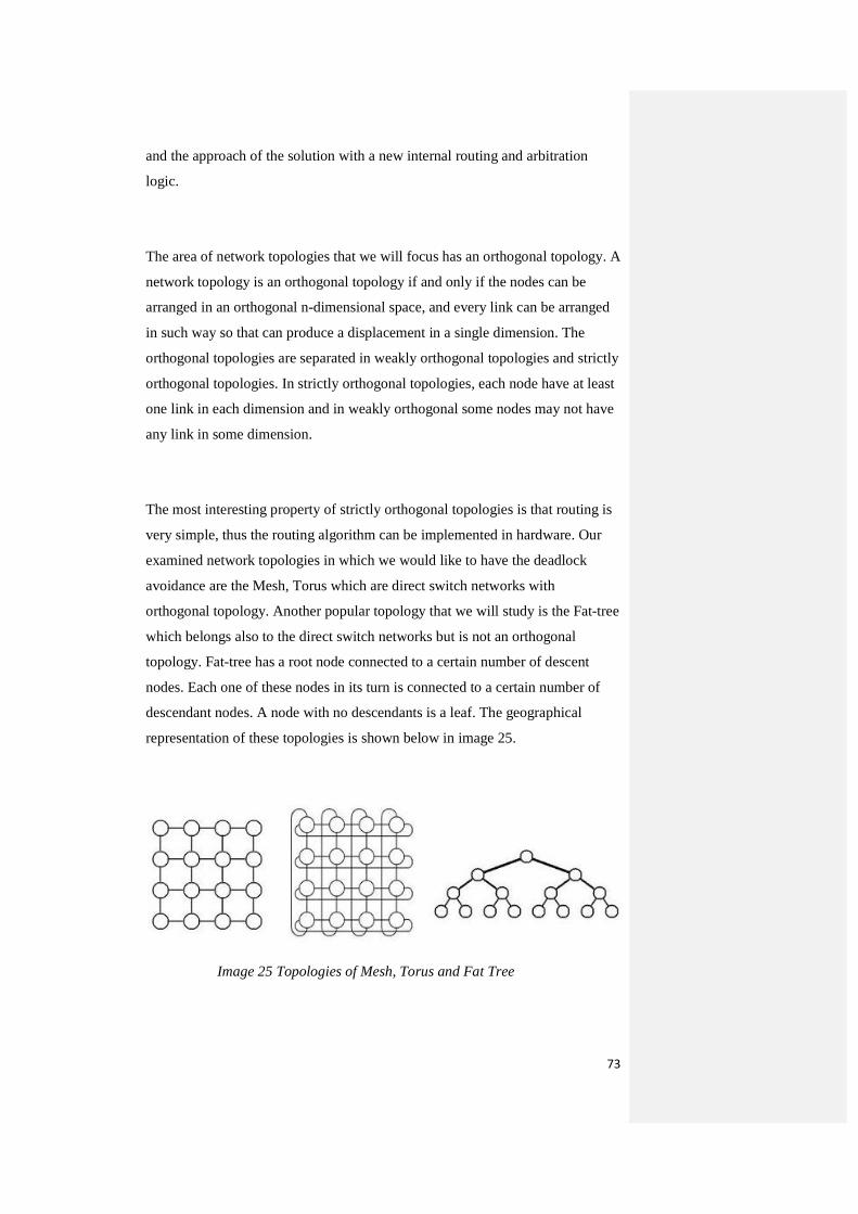
73
and the approach of the solution with a new internal routing and arbitration
logic.
The area of network topologies that we will focus has an orthogonal topology. A
network topology is an orthogonal topology if and only if the nodes can be
arranged in an orthogonal n-dimensional space, and every link can be arranged
in such way so that can produce a displacement in a single dimension. The
orthogonal topologies are separated in weakly orthogonal topologies and strictly
orthogonal topologies. In strictly orthogonal topologies, each node have at least
one link in each dimension and in weakly orthogonal some nodes may not have
any link in some dimension.
The most interesting property of strictly orthogonal topologies is that routing is
very simple, thus the routing algorithm can be implemented in hardware. Our
examined network topologies in which we would like to have the deadlock
avoidance are the Mesh, Torus which are direct switch networks with
orthogonal topology. Another popular topology that we will study is the Fat-tree
which belongs also to the direct switch networks but is not an orthogonal
topology. Fat-tree has a root node connected to a certain number of descent
nodes. Each one of these nodes in its turn is connected to a certain number of
descendant nodes. A node with no descendants is a leaf. The geographical
representation of these topologies is shown below in image 25.
Image 25 Topologies of Mesh, Torus and Fat Tree

Thus in our examination we will see that dealing the deadlock avoidance with
the use of virtual channels, the complexity of the routing mechanism
implemented inside switches increases. For that case we have to consider the
possibilities and the limitations that appear, and the efficient ways with which
we will approach them. In mesh and Fat tree topologies the deadlock avoidance
approach is the same. In Torus topologies thus there are no end nodes, because
of the existence of wrap around links, the complexity of the mechanism
increases allowing to the packets recirculate inside network in all dimensions.
A mesh network has the same node degree but half of the bisectional channels
as a torus with the same radix and dimension. Although Mesh has a natural 2D
geographical representation that keeps channel length short it gives up the edge
symmetry of torus. This can cause imbalance in many traffic patterns, as the
demand from the packets on the resources can increase significantly in the
central channels that the edge channels.
A small analysis follows on a simple 4x4 Mesh network. In image 26a several
source nodes indicated by S, sending packets to equal destination nodes
indicated by D. The routing mechanism provided changing the routing
directions on the packets from XY to YX routing, causing in the central part of
the network deadlock to occur. Blocked packets in the buffers of the switches,
do not allow upcoming packets to pass and reach their destinations. Now the
network is paralyzed and the packets cannot advance due to previous blocked
packets.
On contrary in image 26b, is shown the same 4x4 Mesh network but only this
time using Dimension Order routing (DOR) with the use of virtual channels.
Packets are sended by their source nodes to their equal destination nodes
following this time DOR. That means that the packets are forwarded by the
switches in one dimension, and they change their routing function from XY to
YX or the opposite, only when the reach the coordination of their destination
node. The use of the virtual channels in the internal structure of the switches

75
helps the traversal of the packets which move in the same coordinates of the
network.
Our switch model is using the dimension Order Routing (DOR). Based on that we
have to see how the DOR works and what makes the appearance of Deadlock. DOR is
a deterministic routing algorithm, meaning that is always choose the same path x and
y, even there are multiple possible paths. The algorithm ignores the path diversity of
the underlying topology and because of that makes poor job on balancing the load of
packets. Despite this t is very common in practice thus it’s easy to implement and
easy to make it deadlock free.
The functionality of DOR in Mesh and Hypercube topologies is to establish an order
on all the resources based on network dimension. In Torus and Rings which are
topologies with wrap around links, DOR has to establish an order on all resources
between and within each dimension, and also apply multiple virtual channels for each
physical channel. An alternative approach is to maintain the resources along each
dimension, from reaching their full capacity by ensuring the existence of bubbles.
Image 26 Deadlock avoidance in a 4x4 Mesh
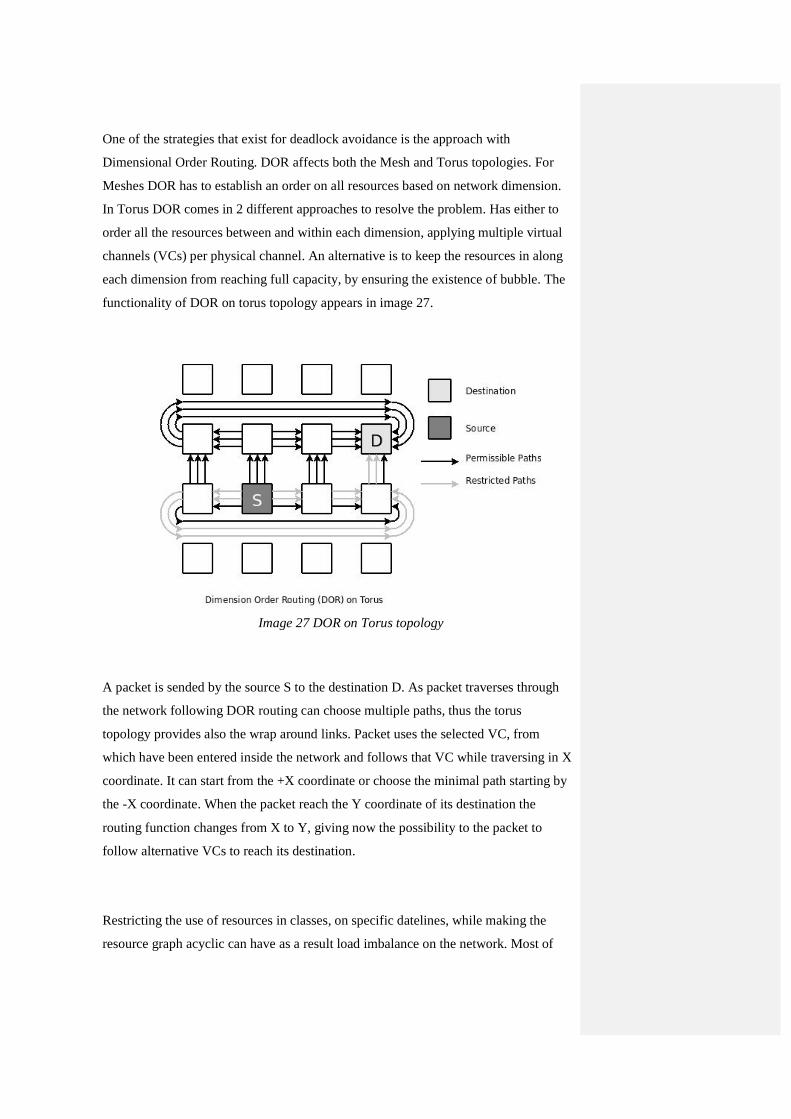
One of the strategies that exist for deadlock avoidance is the approach with
Dimensional Order Routing. DOR affects both the Mesh and Torus topologies. For
Meshes DOR has to establish an order on all resources based on network dimension.
In Torus DOR comes in 2 different approaches to resolve the problem. Has either to
order all the resources between and within each dimension, applying multiple virtual
channels (VCs) per physical channel. An alternative is to keep the resources in along
each dimension from reaching full capacity, by ensuring the existence of bubble. The
functionality of DOR on torus topology appears in image 27.
A packet is sended by the source S to the destination D. As packet traverses through
the network following DOR routing can choose multiple paths, thus the torus
topology provides also the wrap around links. Packet uses the selected VC, from
which have been entered inside the network and follows that VC while traversing in X
coordinate. It can start from the +X coordinate or choose the minimal path starting by
the -X coordinate. When the packet reach the Y coordinate of its destination the
routing function changes from X to Y, giving now the possibility to the packet to
follow alternative VCs to reach its destination.
Restricting the use of resources in classes, on specific datelines, while making the
resource graph acyclic can have as a result load imbalance on the network. Most of
Image 27 DOR on Torus topology
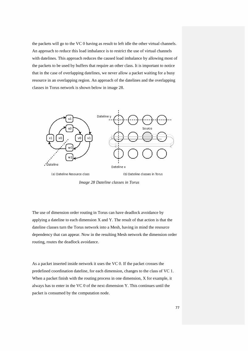
77
the packets will go to the VC 0 having as result to left idle the other virtual channels.
An approach to reduce this load imbalance is to restrict the use of virtual channels
with datelines. This approach reduces the caused load imbalance by allowing most of
the packets to be used by buffers that require an other class. It is important to notice
that in the case of overlapping datelines, we never allow a packet waiting for a busy
resource in an overlapping region. An approach of the datelines and the overlapping
classes in Torus network is shown below in image 28.
The use of dimension order routing in Torus can have deadlock avoidance by
applying a dateline to each dimension X and Y. The result of that action is that the
dateline classes turn the Torus network into a Mesh, having in mind the resource
dependency that can appear. Now in the resulting Mesh network the dimension order
routing, routes the deadlock avoidance.
As a packet inserted inside network it uses the VC 0. If the packet crosses the
predefined coordination dateline, for each dimension, changes to the class of VC 1.
When a packet finish with the routing process in one dimension, X for example, it
always has to enter in the VC 0 of the next dimension Y. This continues until the
packet is consumed by the computation node.
Image 28 Dateline classes in Torus
4.2.1 Network Elements
Important network elements in which we have also to focus and will complete
our network construction are the compute nodes, and the packet structure. The
compute nodes are the elements that produce, consume and taking information
from the packets. For the packet we will examine which are the parts that
complete the structure of the packet and what additions we have to make in
order the packets to follow our routing decisions using the virtual channels.
4.2.1.1 Compute Node
Our compute node models are responsible to generate packets inserting in their
header the appropriate informations like a packet id, receiving the id of the
packet and calculating the latency of the packet. Thus these computational node
models will work as senders and receivers there are several steps that we need to
follow. Important steps for the creation of the node and its functionality, so that
can send a packet to a destination node over the network are listed below.
Sender
� The application layer of the node executes a system call which copies data to be
sent, into a network interface buffer, and composes the header and trailer of the
packet.
� The checksum is calculated and inserted also in the header or trailer of the
packet.
79
� The timer starts and the packet is inserted through the network hardware
interface into the physical layer.
The sender has to react also in case that receives an acknowledgment packet.
The steps for that procedure follow bellow.
� When the sender receive an acknowledgment packet releases the copy of that corresponding packet from the buffer.
� If the sender reaches the timeout instead of receiving an acknowledgment packet, it resends the packet and restarts the timer.
Receiver
Message reception is in the receiver part of nodes network interface
� Network interface receives the packet from the physical layer, and puts it into
the input buffers of the network interface or system buffer.
� Checksum is calculated for each message. If the checksum matches the senders
checksum the receiver send and acknowledgment packet to the packet sender. If
not, deletes the packet assuming that the sender will resend the packet after the
associated time expiration.
� Once all packets pass the test, the system copies data to the system address
space and signals the corresponding application.
4.2.1.2 Packet
The packet is the basic unit of information that is sent from the sender part of
the source computation node to the receiver part of the destination computation
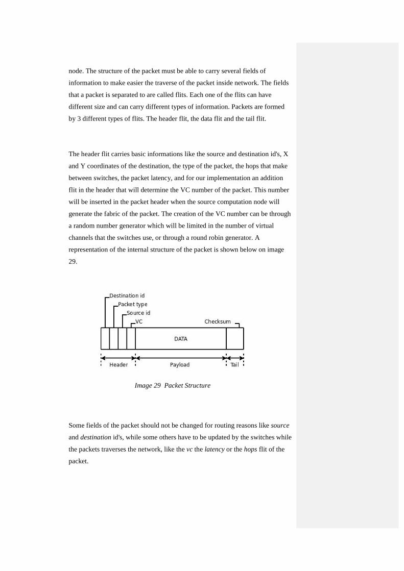
node. The structure of the packet must be able to carry several fields of
information to make easier the traverse of the packet inside network. The fields
that a packet is separated to are called flits. Each one of the flits can have
different size and can carry different types of information. Packets are formed
by 3 different types of flits. The header flit, the data flit and the tail flit.
The header flit carries basic informations like the source and destination id's, X
and Y coordinates of the destination, the type of the packet, the hops that make
between switches, the packet latency, and for our implementation an addition
flit in the header that will determine the VC number of the packet. This number
will be inserted in the packet header when the source computation node will
generate the fabric of the packet. The creation of the VC number can be through
a random number generator which will be limited in the number of virtual
channels that the switches use, or through a round robin generator. A
representation of the internal structure of the packet is shown below on image
29.
Some fields of the packet should not be changed for routing reasons like source
and destination id's, while some others have to be updated by the switches while
the packets traverses the network, like the vc the latency or the hops flit of the
packet.
Image 29 Packet Structure

81
4.2.1.3 Switch michroarchitecture
The subject that we have to deal with is the Deadlock avoidance inside a switch,
with the use of virtual channels. As we have referred in the theory chapter, we
need to eliminate any circular dependencies that exist from the packets to the
buffers. For that we have to focus on the switch architecture with which our
switch model is structured. We have to focus in the way that the switch provides
access to the agents over resources, meaning the packets over the buffers. Thus
our implementation is going to use virtual channels, it means that the number of
entrances and exits of the switch increases, and is now equal with the number of
ports that we use multiplied by the number of virtual channels that each port
hosts.
An example of the increased complexity inside the architecture of the switch
with the use of 2 virtual channels is shown at image 30. Each one of the input
and output ports now hosts 2 VC increasing with that way the number of input
Image 30 Pipelined Switch michroarchitecture with 2VC
buffers and the equal lines that connect them with the routing mechanism in
stage 2 and with the crossbar unit in stage 4. The same also happens and in stage
5 where equal output buffers are partioned in virtual channels.
Now the complexity of the routing mechanism increases thus the competing
packets for an exit port may also compete for the same virtual channel. We
should consider the complexity of the mechanism changing equally the central
routing mechanism, mean the routing, arbitration and crossbar units logic, so
that they can support the new architecture and avoid Deadlock.
The virtual channel switch and node models that have implemented are based on
the previous switch model that has explained in chapter 4.2 and uses single
input and output buffers. The logic in the virtual channel implementation is not
only the partioning of the input and output buffers in 4 virtual channels for one
buffer, but also the altered logic in the central routing mechanism of the switch
so that can respectively support the use of virtual channels. Based on the
internal architecture pipeline we will explain briefly the traversal of the packets
inside switch in stages, the port and VC allocation mechanisms and the
necessary actions in case of competing packets for the same output port and
virtual channel. In our case we make use of the virtual cut through switching,
means that the mechanism is applied in packet level and not in flit level.
Routing computation
Our virtual channel switch for the efficient allocation of an output port and
virtual channel for a newly incoming packet in the switch should make use of 2
state field tables. These tables are the input and output virtual channels state
tables, which contain information about the route computation and virtual
channel allocation of the switch. The first is 5-vector GROPC state table that
has informations for the input virtual channels state and the second is a 3-vector
GIC state table which has informations for the output virtual channels state.
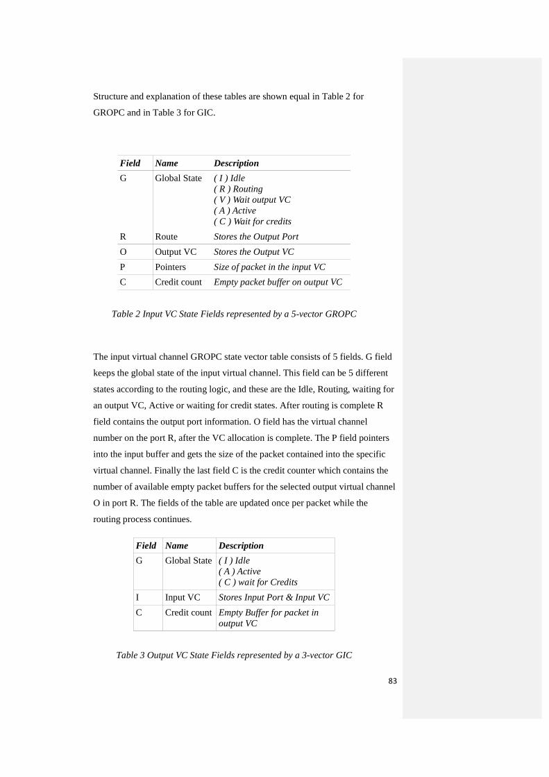
83
Structure and explanation of these tables are shown equal in Table 2 for
GROPC and in Table 3 for GIC.
Field Name Description
G Global State ( I ) Idle ( R ) Routing ( V ) Wait output VC ( A ) Active ( C ) Wait for credits
R Route Stores the Output Port
O Output VC Stores the Output VC
P Pointers Size of packet in the input VC
C Credit count Empty packet buffer on output VC
Table 2 Input VC State Fields represented by a 5-vector GROPC
The input virtual channel GROPC state vector table consists of 5 fields. G field
keeps the global state of the input virtual channel. This field can be 5 different
states according to the routing logic, and these are the Idle, Routing, waiting for
an output VC, Active or waiting for credit states. After routing is complete R
field contains the output port information. O field has the virtual channel
number on the port R, after the VC allocation is complete. The P field pointers
into the input buffer and gets the size of the packet contained into the specific
virtual channel. Finally the last field C is the credit counter which contains the
number of available empty packet buffers for the selected output virtual channel
O in port R. The fields of the table are updated once per packet while the
routing process continues.
Field Name Description
G Global State ( I ) Idle ( A ) Active ( C ) wait for Credits
I Input VC Stores Input Port & Input VC
C Credit count Empty Buffer for packet in output VC
Table 3 Output VC State Fields represented by a 3-vector GIC
The output virtual channel state vector GIC table consists of 3 fields. The global
state field has 3 different states for the output virtual channel buffer which are
the Idle, Active or waiting for Credits. The field I contain the number of the
input port and virtual channels that forward packets to this output virtual
channels. Finally the C field has the number of available free packet buffer for
the packet in the selected output virtual channel.
Stage 1
As shown in Image 4.5 in stage 1, the packets arrive to the switch from the
physical level and received by the receivers in the input ports. The packets
according to their virtual channel number which is stored in the VC header flit,
are directed and stored in the appropriate input virtual channels of the switch.
Now from stage 1 the input virtual channel informs the routing unit so that can
start the routing process and allocate an output port and an output virtual
channel for the packet. The global state (G) field of the GROPC table which
was Idle until now for the specific VC, turns to (G=R).
Stage 2
In stage 2 of the pipeline the information from the header of the packet is used
by the router to select an output port. The result of this computation updates the
route R field of the GROPC table with number of the selected output port and
advances the global state (G) of the packet in waiting for an output virtual
channel (G=V). Both actions happen at the start of Stage 3 in VC switch
pipeline.
Stage 3
During stage 3 the result of the routing computation information from the
packets header which was stored in the R field of the GROPC table, is used as
input on the Virtual Channel Allocator. If the insertion of the value is
successful, the VC allocator search and assign a single output virtual channel on
the output port specified on the R field of the table. The result of the virtual

85
channel allocation updates the (O) field of the GROPC table with the virtual
channel number and updates also the global state (G) field to the active A state
(G=A).
In stage 3 are also updated and the fields of the GIC table. The result of the
allocation updates the global state G field of the GIC table to an active A state
(G=A), thus until now was in the Idle state. After the channel turns active, the
(I) field is updated with the appropriate information, so that can identify the
input port and virtual channel of the packet. From now and until the release of
the input buffer by packet, the (C) field of the GIC table is also reflected in the
(C) field of the GROPC table.
For the purposes of Deadlock Avoidance, stage 3 where the virtual channel
allocation takes place, is the point at which a dependency is created from the
input virtual channel to the output virtual channel. “After a single output virtual
channel is allocated to the packet, the input virtual channel will not be freed
until the packet is able to move its entire content into the output virtual channel”
[1 ch16]
Stage 4
In the begging of the stage 4, all the “per packet processing” is complete and
remains the crossbar to establish a path between the input virtual channel on the
input port, and the output virtual channel on the output port. In this stage any
active virtual channel (G=A) that contains buffered packet inside of a certain
size, indicated by the field P on GROPC table, and has equal empty packet
buffer space on the output virtual channel (C>0 && C>=P), informs the
crossbar. The active virtual channel bids on crossbar for a connection between
its input virtual channel and the output port that contains its output virtual
channel. Depending on the configuration of the switch this allocation may
involve competition not only for the output port of the switch but also
competition for the specific output virtual channel.
Until the allocation process finish the packet staying stored inside the input
buffers of the switch, thus we don’t treat them as separated flits that progress
with the routing computation and the port and virtual channel allocation.
Stage 5
In that last stage the necessary information has reached the crossbar and the
allocation has performed. When the packet is successfully scheduled, releases
the virtual channel at the start of the stage and is setting the virtual channel state
(G) field of the GIC table to Idle (G=I). The same field (G) for the GROPC
table is also updated to Idle, if the input buffer is empty.
If the input buffer is not empty, information for the next packet that is waiting in
the buffer is issued. In that case the state transition to routing (G=R).
Analysis of Resource Dependencies for Deadlock Avoidance
The analysis for the resource dependencies is focusing on the arbitration unit of
the switch. Inside the arbitration unit are received the numbers of the input port
and input virtual channel that contain the packet and the requested output port
and output virtual channel. Our unit make use of a round robin arbiter which can
provide strong fairness to our switch.
The arbitration unit have to resolve the resource dependencies that occur when
multiple packets request the same resources. This process is done through the 5
stages of the pipeline architecture which is concentrated as control into the
arbitration unit. The arbitration unit passes information into the crossbar and
assures that the input virtual channel in which the packet is stored, will not let
free until the entire packet pass to the calculated output virtual channel and
output port.

87
Image 31 3 phase arbitration
The used arbitration is a 3 phase arbitration technique which consists by 3
phases, the Request, Grand and Acknowledgment phase. We need to make use
of 3 phase arbitration because the increased inputs and outputs of the switch
with the virtual channel implementation, increasing the probability of matching
requests. For an input output buffered switch which each input port has an
associated queue, the output port needs to have a local arbiter with a round robin
strategy. As it seen from the image 31 the arbitration technique starts by
submitting requests to the output port arbiters which receiving the messages and
through the round robin selecting one of the requests. The arbiters now in Grand
phase giving permission to the selected for Grand input port. Thus the requested
for Grand input ports may request for more than one output port, they may
receive more than one Grands. In the last phase, the input ports select one of the
responded output ports and send an Ack to confirm the selection of the output
port. The used 3 phase arbitration provides 75% efficiency thus the 3 of the 4
requests are granted to output ports, in comparison with a 2 phase arbitration
that provides only 50% efficiency.
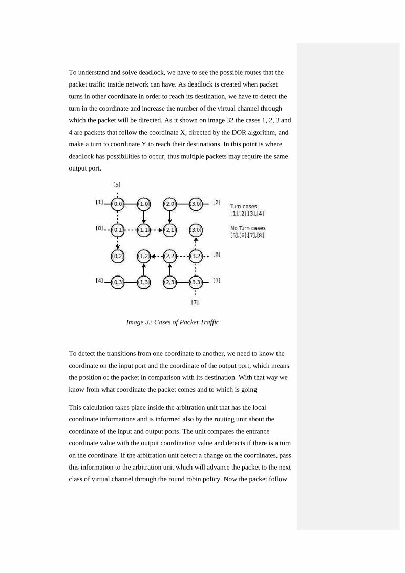
To understand and solve deadlock, we have to see the possible routes that the
packet traffic inside network can have. As deadlock is created when packet
turns in other coordinate in order to reach its destination, we have to detect the
turn in the coordinate and increase the number of the virtual channel through
which the packet will be directed. As it shown on image 32 the cases 1, 2, 3 and
4 are packets that follow the coordinate X, directed by the DOR algorithm, and
make a turn to coordinate Y to reach their destinations. In this point is where
deadlock has possibilities to occur, thus multiple packets may require the same
output port.
Image 32 Cases of Packet Traffic
To detect the transitions from one coordinate to another, we need to know the
coordinate on the input port and the coordinate of the output port, which means
the position of the packet in comparison with its destination. With that way we
know from what coordinate the packet comes and to which is going
This calculation takes place inside the arbitration unit that has the local
coordinate informations and is informed also by the routing unit about the
coordinate of the input and output ports. The unit compares the entrance
coordinate value with the output coordination value and detects if there is a turn
on the coordinate. If the arbitration unit detect a change on the coordinates, pass
this information to the arbitration unit which will advance the packet to the next
class of virtual channel through the round robin policy. Now the packet follow
89
the next in class virtual channels, avoiding to enter in the first virtual channel
which can be used by a packet that travels in one coordinate. From the image 32
we create an offset table based on the offset values from the 3 switches that each
packet passes. With that strategy we avoid the possibility that will occur a
deadlock.

91
5 Design
The design of the switch and node model is through the Opnet network
simulator version 14.5.A. The basic model, in which our implementation is
based, has been created in version 14.0.A of the simulator. In this chapter, it
will be presented the several modules that create a virtual channel switch, how
these are connected between them and what is the function of each module
separately. The explanation of the design will follow the pipeline architecture of
a virtual channel switch, which has explained in the previous chapter of the
analysis. In our model, we make use of 4 virtual channels, providing with that
way 3 more alternative paths for the packets to pass through the switch.
5.1 General Switch Structure
In the virtual channel switch, the partition of the input buffers into virtual
channels cause the need of equal packet stream lines that will connect the input
buffers with the crossbar unit. The internal structure of the switch is presented in
the image 33.The switch architecture consists of several parts. First and basic is
the switch unit that initializes the functions of our switch like the ports. The
input unit, which is at the entrance of the switch, consists of the virtual channel
selection unit and the input virtual channel buffers. The central mechanism
consists of the routing, arbitration and crossbar units, that all together
accomplish the routing logic of our switch. In the exit of the switch, there are
the output buffers and the forward unit that sends our packets into network.
For the input unit of our switch, the virtual selection unit is connected to the
input virtual channels with four packet wires. This is because the virtual channel
selection unit recognise the vc header on the packet and according to the virtual
channel state sends the packet through the appropriate channel. The same design
in connections also follows the input virtual channel buffers which are
connected with the crossbar unit, through packet wires, equal with the virtual
channels.
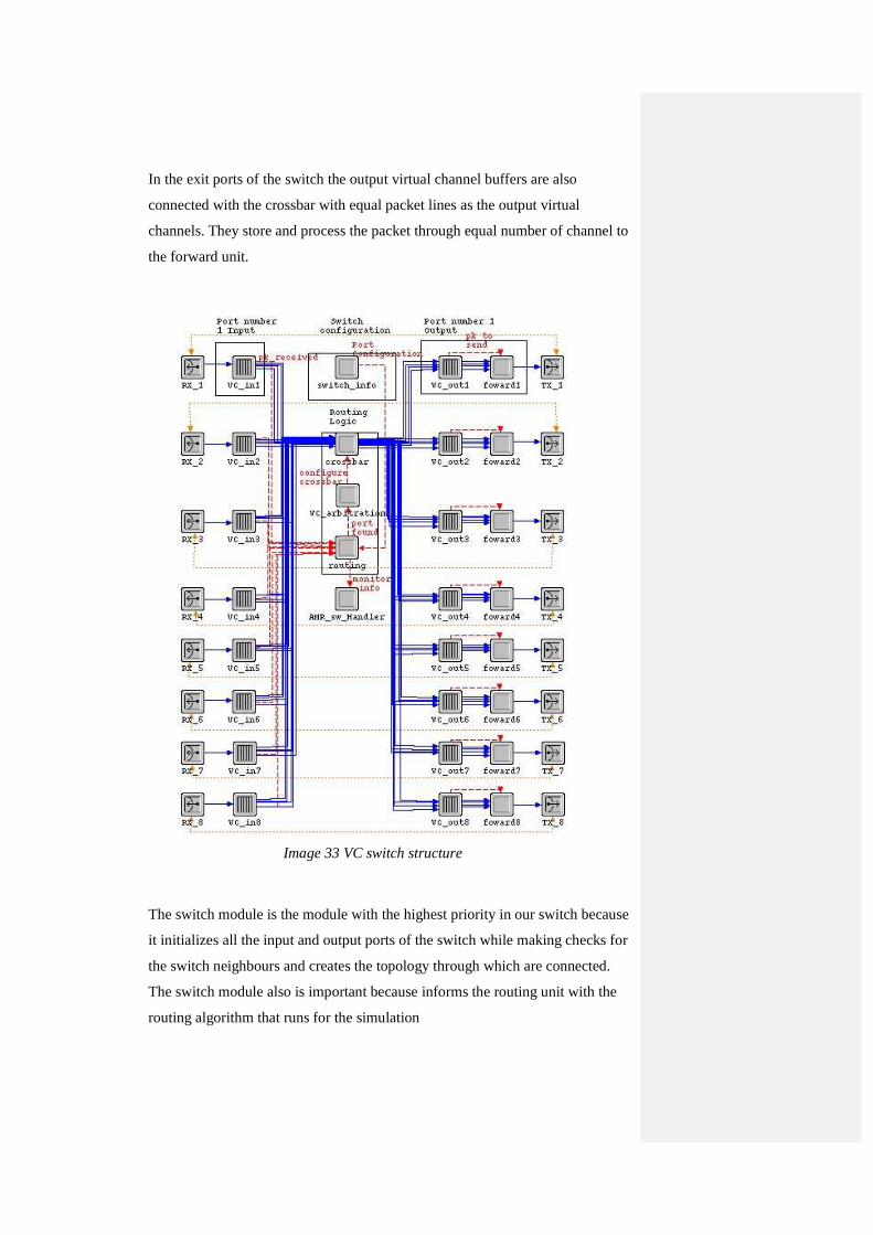
In the exit ports of the switch the output virtual channel buffers are also
connected with the crossbar with equal packet lines as the output virtual
channels. They store and process the packet through equal number of channel to
the forward unit.
The switch module is the module with the highest priority in our switch because
it initializes all the input and output ports of the switch while making checks for
the switch neighbours and creates the topology through which are connected.
The switch module also is important because informs the routing unit with the
routing algorithm that runs for the simulation
Image 33 VC switch structure

93
In the central part of the switch the routing module is responsible to receive
information from the input virtual channel buffers about the packet that are
waiting to be routed. The routing unit have to calculate the appropriate output
port and inform the Virtual Channel Arbitration unit. The virtual channel
arbitration unit is receiving that informations and after the necessary
calculations that will resolve any resource dependencies which may occur, pass
the information to the crossbar. Now the crossbar using the information will
establish a link between the input and the output virtual channels, so that the
packet can pass.
5.1.1 Input Virtual Channel Buffers
The input virtual channel buffers are the unit that contains our virtual channels
into it. The module, for the representation of the virtual channels, provides the
advantage of having finite or infinite buffer size for our virtual channels. The
module is connected with the receiver of the switch so that can receive the
incoming packet from the physical layer and with the crossbar through packet
streams equal to the number of our subqueue, in our case four. The internal
states of the module are shown below in image 34.
Init
Unit starts with the init process where initialize the functions that will use. It
starts with registering the local statistic that is going to use for the
Image 34 Input virtual channel buffers

communication with the routing unit. Next the unit receive the input port and
the number of the subqueue in which is partitioned and allocates dynamically a
space on the memory to store the current outgoing packets. After the
initialization proceed to the next BRANCH state.
Branch
The module now pass through an empty condition to the Branch state where is
idle, waiting an interrupt to occur. Depending on the type of interrupt or the
value that the interrupt it carries, the module proceed to the corresponding state.
Ins_Tail
The first state that is enabled with a stream interrupt is the INS_TAIL. Here the
module receives the packet from the incoming stream and read its virtual
channel number from its header. Next the state receives the size of the packet
and the packet id and check if the subqueue which corresponds to the virtual
channel number is empty. If the subqueue is empty, the packet is inserted in the
tail of the subqueue and the module inform the routing unit, through a statistic
wire, that a packet has inserted in the specific port and the specific virtual
channel subqueue.
Send_Head
This state is the next that is enabled with an access interrupt by the crossbar.
Here the state makes a check in the subqueue, for the specific virtual channel
number, to see if it has a waiting packet in the head. If it is, the state making
access to the head of the subqueue to receive the packet while calculates the
latency of the buffer. The packet is removed from the head of the subqueue and
the size of it and its id are stored before the state send the packet to the crossbar
unit. The state here for simulation reasons and based on the internal bandwidth
of the switch, the switch delay and the packet size, it calculates the time that the
packet needs to entirely leave the subqueue. Based on this time causes a self
interrupt that passes the module to the next state.
PkSENT
The PkSENT state is enabled with the self interrupt of the Send_Head state after
the small time delay. Now a second check is made to the subqueue to see if new
packet has reached the Head of the subqueue while the last packet was leaving.

95
If in the head exist a packet the unit informs once more the routing unit through
a statistic for the input port and subqueue in which the packet is stored.
END_SIM
This state is inactive and is activated only if we need to, with an exit interrupt.
The state is used only to store simulation information into a text file.
5.1.2 Routing Unit
The routing unit is the responsible unit that will find an exit port to our packet
based on the current position of the switch, the destination information that the
packet carries and the routing algorithm that our switch uses. The unit is
connected with statistic wires with every input port of our switch to receive
information about the packets that waiting to be routed, with the arbitration unit
in which will pass the calculated output port number and finally with the switch
unit of our switch from which receives the forward tables that will use. The
internal structure of the routing unit is shown on the image 35.
Init
The routing unit begins its function by initializing the necessary variables in the
unforced state Init. Here the unit receives information about the connected to its
ports, the internal bandwidth of the switch. Here is also allocated and initialized
a structure that will be used with a round robin strategy to search between the
Image 35 Routing unit
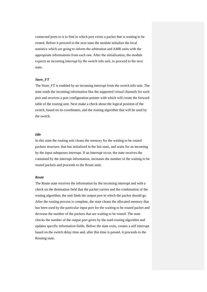
connected ports to it to find in which port exists a packet that is waiting to be
routed. Before it proceed to the next state the module initialize the local
statistics which are going to inform the arbitration and AMR units with the
appropriate informations from each one. After the initialization, the module
expects an incoming interrupt by the switch info unit, to proceed to the next
state.
Store_FT
The Store_FT is enabled by an incoming interrupt from the switch info unit. The
state reads the incoming information like the supported virtual channels for each
port and receives a port configuration pointer with which will create the forward
table of the routing unit. Next make a check about the logical position of the
switch, based on its coordinates, and the routing algorithm that will be used by
the switch.
Idle
In this state the routing unit cleans the memory for the waiting to be routed
packets structure, that has initialized in the Init state, and waits for an incoming
by the input subqueues interrupt. If an interrupt occur, the state receives the
contained by the interrupt information, increases the number of the waiting to be
routed packets and proceeds to the Route state.
Route
The Route state receives the information by the incoming interrupt and with a
check on the destination field that the packet carries and the combination of the
routing algorithm; the unit finds the output port in which the packet should go.
After the routing process is complete, the state cleans the allocated memory that
has been used by the particular input port for the waiting to be routed packet and
decrease the number of the packets that are waiting to be routed. The state
checks the number of the output port given by the used routing algorithm and
updates specific information fields. Before the state exits, creates a self interrupt
based on the switch delay time and, after this time is passed, it proceeds to the
Routing state.
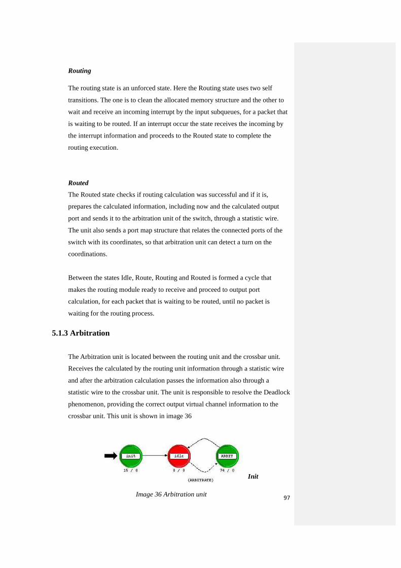
97
Routing
The routing state is an unforced state. Here the Routing state uses two self
transitions. The one is to clean the allocated memory structure and the other to
wait and receive an incoming interrupt by the input subqueues, for a packet that
is waiting to be routed. If an interrupt occur the state receives the incoming by
the interrupt information and proceeds to the Routed state to complete the
routing execution.
Routed
The Routed state checks if routing calculation was successful and if it is,
prepares the calculated information, including now and the calculated output
port and sends it to the arbitration unit of the switch, through a statistic wire.
The unit also sends a port map structure that relates the connected ports of the
switch with its coordinates, so that arbitration unit can detect a turn on the
coordinations.
Between the states Idle, Route, Routing and Routed is formed a cycle that
makes the routing module ready to receive and proceed to output port
calculation, for each packet that is waiting to be routed, until no packet is
waiting for the routing process.
5.1.3 Arbitration
The Arbitration unit is located between the routing unit and the crossbar unit.
Receives the calculated by the routing unit information through a statistic wire
and after the arbitration calculation passes the information also through a
statistic wire to the crossbar unit. The unit is responsible to resolve the Deadlock
phenomenon, providing the correct output virtual channel information to the
crossbar unit. This unit is shown in image 36
Init
Image 36 Arbitration unit
In Init state, the module initializes the local statistic that going to use, to pass its
calculated information to the crossbar unit. After the initialization, it proceeds to
the next state.
Idle
Here the module is waiting for an incoming interrupt by the routing unit. If an
interrupt occurs, the module pass to the next state where it will begin the
arbitration process.
ARBIT
In the Arbit state, the unit receives the incoming by the routing unit information.
The unit based on the input and output port numbers that have received,
calculates the streams through which the crossbar will receive the packets from
the input subqueues and through which stream will send them to the
corresponding output ports. In this state also the arbitration checks if between
the input and output ports exists a turn on the coordinations from X to Y or the
opposite. If the state detects a turn, changes the number of the virtual channel
providing with that way the deadlock avoidance policy that we need for our
Mesh models. The state prepare the information like the input and output
streams and the input and output virtual channels and send this information
through a statistic wire to the crossbar. The Deadlock Avoidance policy that
detects the turn on the coordinations is shown on the table 4.
// HERE DETECT A TURN ON THE COORDINATE If( (((output_port == y_negative) || (output_port == y_positive)) && ((input_port == x_negative) || (input_port == x_positive))) || ((output_port == x_negative) || (output_port == x_positive)) && ((input_port == y_negative) || (input_port == y_positive)) ) { if (input_vc==3) output_vc=0; else output_vc = input_vc++ } // NO TURN ON THE COORDINATE HAVE DETECTED If(((output_port == y_negative) && (input_port == y_positive)) || ((output_port == y_positive) && (input_port == y_negative)) || ((output_port == x_negative) && (input_port == y_positive)) || ((output_port == x_positive) && (input_port == x_negative)) ||

99
{ output_vc = input_vc; })
Table 4 Deadlock Avoidance Policy
In the Deadlock Avoidance policy that is shown on table 4, the unit receives the
coordinate values from the input port that the packet has entered inside switch
and compare that value with the coordinate value of the output port that the
packet needs. The unit now is able to detect the change on the coordinate and if
that happen, increase the class of the virtual channel field through a round robin
algorithm.
For the case of torus that we need the dateline policy. Here the module checks
the logical position of the switch and in case that the switch is in the dateline
limits of our network, the module provides the dateline policy that affect the
virtual channel fields. A sample of the code that is included in this module for
the dateline classes in the X an Y coordinates of a torus topology, follows below
on table 5.
op_ima_obj_attr_get (node, “X”, &x_label);
op_ima_obj_attr_get (node, “Y”, &y_label);
if ((x_label==0) || (y_label==0))
{ if (vc==3) {vc=0;}
else vc++;
}
Table 5 Dateline classes for Torus
In the code that is shown on table 5, the state receives the logical local
coordinates of the switch and checks if these coordinates mach with the dateline
coordinates of the topology, meaning the coordinate X=0 and Y=0. If the check
detects that the packet pass from those coordinates, make a check on the virtual
channel header flit of the packet and increase the virtual channel number
through a round robin calculation.
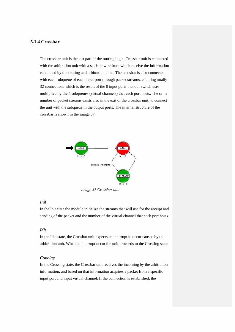
5.1.4 Crossbar
The crossbar unit is the last part of the routing logic. Crossbar unit is connected
with the arbitration unit with a statistic wire from which receive the information
calculated by the routing and arbitration units. The crossbar is also connected
with each subqueue of each input port through packet streams, counting totally
32 connections which is the result of the 8 input ports that our switch uses
multiplied by the 4 subqueues (virtual channels) that each port hosts. The same
number of packet streams exists also in the exit of the crossbar unit, to connect
the unit with the subqueue in the output ports. The internal structure of the
crossbar is shown in the image 37.
Init
In the Init state the module initialize the streams that will use for the receipt and
sending of the packet and the number of the virtual channel that each port hosts.
Idle
In the Idle state, the Crossbar unit expects an interrupt to occur caused by the
arbitration unit. When an interrupt occur the unit proceeds to the Crossing state
Crossing
In the Crossing state, the Crossbar unit receives the incoming by the arbitration
information, and based on that information acquires a packet from a specific
input port and input virtual channel. If the connection is established, the
Image 37 Crossbar unit

101
Crossbar unit that received the packet, reads the information carried by the
packet fields and if it is needed updates some fields. After this calculation, the
unit passes the packet to the corresponding output stream that will lead the
packet to the output port calculated by the routing algorithm and the output
virtual channel calculated by the arbitration unit.
5.1.5 Output Virtual Channel Buffers
The output virtual channel buffers are located in the last part of the switch after
the crossbar unit. The unit is connected with the crossbar with packet streams
equal to the number of the virtual channel subqueues that hosts, and has equal
packet stream connections with the forward unit after it. Also a statistic wire
from the output virtual channel buffers informs the next unit that a packet is
ready to be sent from the buffers to the physical layer. The internal structure of
the output virtual channel buffers is show at the image 38.
Init
In the Init state, the unit receives the number of the supported ports by the
switch, the number of the specific port in which it is and the number of the
subqueues hosted by the buffer. Before exit the Init state, the unit allocates a
space in the memory for the outgoing packets by the unit and initialize the local
statistic through which will inform the forward unit for an outgoing packet.
Image 38 Output virtual channel buffers
Ins_Tail
In the Ins_tail state, the unit receives the incoming packet by the input stream
and reads the virtual channel number that the packet carries in its VC field. The
unit obtains the packet size and checks if the subqueue with the same number as
the virtual channel field is empty. If the subqueue is empty, the unit insert the
packet to the tail of the subqueue and informs through a statistic wire the
forward unit that the specific subqueue has a packet. Then returns to the idle
state where waits for the next interrupt to occur and have access at the Head of
the subqueue.
Send_Head
In the Send_Head state, the unit receives the access request to access the
specific subqueue. The unit checks if the requested subqueue is empty and if it’s
not, it access the first packet that is on the Head of the subqueue, and gets the
size of that packet. Next the unit calculates the latency for the specific subqueue
and removes the packet from its Head. The unit sends the removed packet by
the subqueue and sends it to the forward unit without causing an interrupt,
because earlier had informed the forward unit through the statistic wire. The
unit based on the packet size and the bandwidth of its line, calculates the time
that the packet needs to entirely leave the subqueue and based on that time
creates a self interrupt that will lead the unit to the next state.
PkSENT
After the expiration time of the caused interrupt the unit enters the PkSENT
state. Here the unit makes a second check to the head of the subqueue to see if a
new packet has arrived in the Head of the subqueue while the last was leaving
the subqueue. If a new packet has reached the subqueue the unit informs once
more the forward unit through the statistic wire.
5.1.6 Forward unit The forward unit is the last unit of the switch before the packets are sended to
the physical layer. The unit is connected with the output virtual buffers with four
packet wires through which will receive the packet and also with a statistic wire
from which is informed when a packet is entering or leaving a subqueue. The
unit is also connected with the transmitter of the switch through a packet stream

103
to pass the packets to the physical layer. The internal structure of the forward
unit is shown below in the image 39.
Init
In the Init state the unit makes the necessary initialization, by receiving the port
number in which the unit is located. Also in the init state is allocated a structure
on the memory so that can hold in each subqueue of the output virtual channel
buffers are packets that waiting to be forward. When the unit finish with the
initialization process, proceeds to the idle state where waits for the next
interrupt to occur.
Receiving
This state is enabled first by the statistic interrupt that connect the unit with the
output virtual channel buffers. The forward unit is informed that a packet exists
in the head of the subqueue and wants to be forward to the physical layer. Here
the unit informs the allocated structure table for the subqueue that has the packet
stored. The unit calculates the time that the packet needs to be forward and
makes a self interrupt based on this time delay, to proceed on the next state.
Send
After the small delay the unit enters the Send state. Here the unit make access to
the requested stream that caused the interrupt and after a small check to the
stream, to see if its empty, receive the packet from the specific subqueue and
forwards it to the physical layer.
Image 39 Forward unit

105
6 Experimentation and Simulation results
In the 6th chapter, we will view the experimentation design for the three
topologies and the strategy that we will follow to create and study the deadlock
phenomenon. Different configurations will be examined for the topologies of
Fat Tree, Torus and Mesh topologies. The collected results will be evaluated so
that we can see the efficiency of the inserted Deadlock avoidance mechanism, in
comparison with the increased latency that causes to the data traffic of the three
networks.
6.1 System Details
The simulation models and the simulation process have taken place in a
personal laptop that running an Ubuntu 8.04 operating system, with Opnet
modeller version 14.5.A installed.
In our Opnet switch models, we set the size of the input and output virtual
channels of the switch in the minimum size of packets that they can accept. In
detail, the size of each virtual channel is set to the minimum, so that can accept
only one packet of 1024 bits for each virtual channel. With that configuration
we increase the probability that more than one packet has the need for the same
buffer resources, and because it has the buffers at the minimum size, we force
the network to produce a deadlock on these resources.
Each simulation will run for packet load from 200 to 4000 Mbps / node with a
step of 200 Mbps / node for each topology. Through this we will observe how
each topology reacts for the same amount of load and in case of torus with
different deadlock configuration. The size of the Mesh and Torus topologies will
be 4x4, and for the Fat Tree we will use a tree with 16 end nodes.
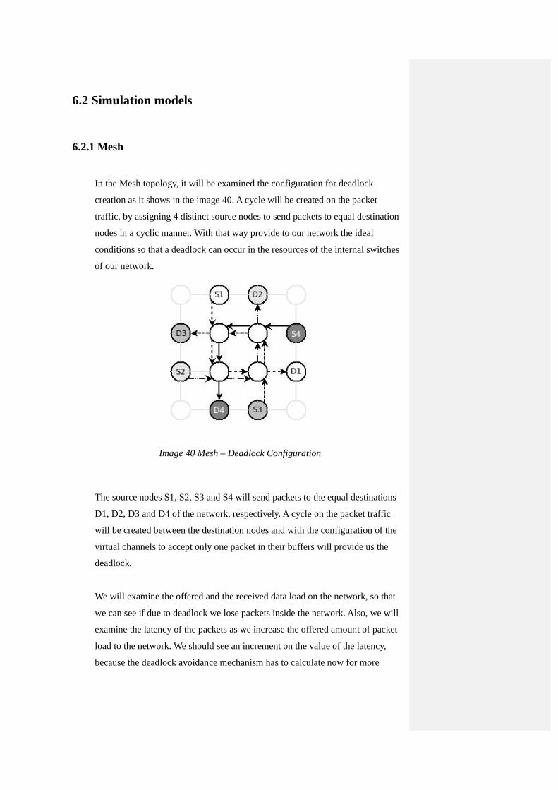
6.2 Simulation models
6.2.1 Mesh
In the Mesh topology, it will be examined the configuration for deadlock
creation as it shows in the image 40. A cycle will be created on the packet
traffic, by assigning 4 distinct source nodes to send packets to equal destination
nodes in a cyclic manner. With that way provide to our network the ideal
conditions so that a deadlock can occur in the resources of the internal switches
of our network.
The source nodes S1, S2, S3 and S4 will send packets to the equal destinations
D1, D2, D3 and D4 of the network, respectively. A cycle on the packet traffic
will be created between the destination nodes and with the configuration of the
virtual channels to accept only one packet in their buffers will provide us the
deadlock.
We will examine the offered and the received data load on the network, so that
we can see if due to deadlock we lose packets inside the network. Also, we will
examine the latency of the packets as we increase the offered amount of packet
load to the network. We should see an increment on the value of the latency,
because the deadlock avoidance mechanism has to calculate now for more
Image 40 Mesh – Deadlock Configuration
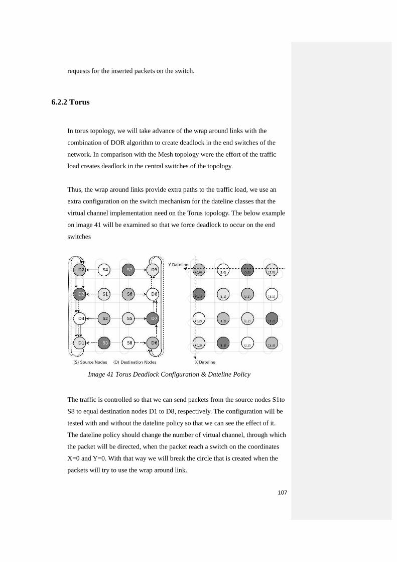
107
requests for the inserted packets on the switch.
6.2.2 Torus
In torus topology, we will take advance of the wrap around links with the
combination of DOR algorithm to create deadlock in the end switches of the
network. In comparison with the Mesh topology were the effort of the traffic
load creates deadlock in the central switches of the topology.
Thus, the wrap around links provide extra paths to the traffic load, we use an
extra configuration on the switch mechanism for the dateline classes that the
virtual channel implementation need on the Torus topology. The below example
on image 41 will be examined so that we force deadlock to occur on the end
switches
Image 41 Torus Deadlock Configuration & Dateline Policy
The traffic is controlled so that we can send packets from the source nodes S1to
S8 to equal destination nodes D1 to D8, respectively. The configuration will be
tested with and without the dateline policy so that we can see the effect of it.
The dateline policy should change the number of virtual channel, through which
the packet will be directed, when the packet reach a switch on the coordinates
X=0 and Y=0. With that way we will break the circle that is created when the
packets will try to use the wrap around link.

If we see the example of image 41 separately for each one of the intermediate
switches that each packet has to travel from its source to each destination, we
will create the below tables. These tables map the path for each packet and
showing the change of virtual channel when the dateline policy is applied to the
switches. The selected dateline is the axis Y=0. When the packets pass from that
axis, they change virtual channel breaking with that way the circular
dependency.
Virtual channel
at Switch 1
Virtual channel
at Switch 2
Virtual channel
at Switch 3
Virtual channel
at Switch 4
Source 1 0 0 0 0 Destination 1
Source 2 0 0 0 0 Destination 2
Source 3 0 0 0 0 Destination 3
Source 4 0 0 0 0 Destination 4
Table 6 Torus without the use of VC
In table 6 we see that all the packet s that travel inside network use the virtual
channel 0, making with that way a dependency to create between the resources
that the packets want to access on the switches. This dependency cycle is
avoided with the use of the dateline policy.
Virtual channel
at Switch 1
Virtual channel
at Switch 2
Virtual channel
at Switch 3
Virtual channel
at Switch 4
Source 1 0 0 0 0 Destination 1
Source 2 0 0 0 1 Destination 2
Source 3 0 0 1 1 Destination 3
Source 4 1 1 1 1 Destination 4
Table 7 Torus with the use of VC
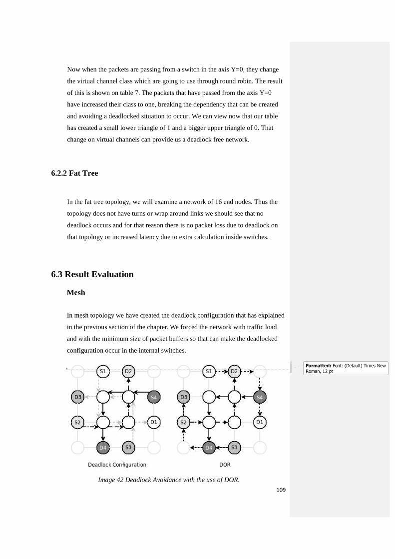
109
Now when the packets are passing from a switch in the axis Y=0, they change
the virtual channel class which are going to use through round robin. The result
of this is shown on table 7. The packets that have passed from the axis Y=0
have increased their class to one, breaking the dependency that can be created
and avoiding a deadlocked situation to occur. We can view now that our table
has created a small lower triangle of 1 and a bigger upper triangle of 0. That
change on virtual channels can provide us a deadlock free network.
6.2.2 Fat Tree
In the fat tree topology, we will examine a network of 16 end nodes. Thus the
topology does not have turns or wrap around links we should see that no
deadlock occurs and for that reason there is no packet loss due to deadlock on
that topology or increased latency due to extra calculation inside switches.
6.3 Result Evaluation
Mesh
In mesh topology we have created the deadlock configuration that has explained
in the previous section of the chapter. We forced the network with traffic load
and with the minimum size of packet buffers so that can make the deadlocked
configuration occur in the internal switches.
Image 42 Deadlock Avoidance with the use of DOR.
Formatted: Font: (Default) Times NewRoman, 12 pt

As we use the Dimension Order Routing (DOR), the traffic load is directed first
on the axis X and when it reaches the equal coordinate Y as the destination,
makes a turn to this axis. Based on the DOR algorithm, we have seen that we
cannot produce deadlock in mesh topology thus we put an order on the routing
of the packet traffic, eliminating the routing from axis Y to X as a first step. The
turns from Y to X and from X to Y make the traffic of the topology create a
circle and deadlock to occur. Therefore, this configuration has been tested
without the use of the virtual channels because they are not needed.
Torus
In the Torus topology, we forced the system with the deadlock configuration that
has explained on section 6.2.2. The packet buffers of the switch were limited to
the size for 1 packet, so that we can force the network to produce deadlock on
the end switches. The results collected by the simulation without the use of the
dateline policy are shown on the below table 7.
Load Global Offered Load
(Mbps / node)
Global Received Load (Mbps / node)
Latency (sec)
Global Generated packets
(Mbps / node)
Global Received packets
(Mbps / node)
Global Load Difference (Mbps / node)
200 1,00E+008 1,00E+008 1,58E-006 781256 781256 0
400 2,00E+008 2,00E+008 1,58E-006 1,56E+006 1,56E+006 0
600 3,00E+008 3,00E+008 1,58E-006 2,34E+006 2,34E+006 0
800 4,00E+008 4,00E+008 1,58E-006 3,13E+006 3,13E+006 10
1000 5,00E+008 5,00E+008 1,58E-006 3,91E+006 3,91E+006 10
1200 6,82E+008 3,41E+008 1,63E-006 24 12 12
1400 8,03E+008 4,01E+008 1,58E-006 16 8 8
1600 8,65E+008 2,16E+008 1,42E-006 16 4 12
1800 9,20E+008 2,30E+008 1,42E-006 16 4 12
2000 1,45E+009 2,42E+008 1,42E-006 24 4 20
2200 1,45E+009 2,42E+008 1,42E-006 24 4 20
2400 1,45E+009 2,42E+008 1,42E-006 24 4 20
2600 1,45E+009 2,42E+008 1,42E-006 24 4 20
2800 1,45E+009 2,42E+008 1,42E-006 24 4 20
3000 1,94E+009 2,42E+008 1,42E-006 32 4 28
3200 1,94E+009 2,42E+008 1,42E-006 32 4 28
3400 1,94E+009 2,42E+008 1,42E-006 32 4 28
3600 1,94E+009 2,42E+008 1,42E-006 32 4 28
3800 1,94E+009 2,42E+008 1,42E-006 32 4 28
4000 2,42E+009 2,42E+008 1,42E-006 40 4 36
Tablet 7 Deadlock configurations on torus without virtual channels
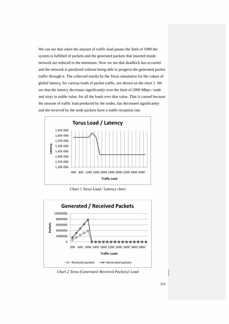
111
We can see that when the amount of traffic load passes the limit of 1000 the
system is fulfilled of packets and the generated packets that inserted inside
network are reduced to the minimum. Now we see that deadlock has occurred
and the network is paralysed without being able to progress the generated packet
traffic through it. The collected results by the Torus simulation for the values of
global latency, for various loads of packet traffic, are shown on the chart 1. We
see that the latency decreases significantly over the limit of 2000 Mbps / node
and stays in stable value, for all the loads over that value. That is caused because
the amount of traffic load produced by the nodes, has decreased significantly
and the received by the node packets have a stable reception rate.
Chart 1 Torus Load / Latency chart
Chart 2 Torus (Generated /Received Packets)/ Load
1,30E-006
1,35E-006
1,40E-006
1,45E-006
1,50E-006
1,55E-006
1,60E-006
1,65E-006
400 800 1200 1600 2000 2400 2800 3200 3600 4000
Late
ncy
Traffic Load
Torus Load / Latency
0
2000000
4000000
6000000
8000000
10000000
200 600 1000 1400 1800 2200 2600 3000 3400 3800
Pa
cke
ts
Traffic Loads
Generated / Received Packets
Received packets Generated packets
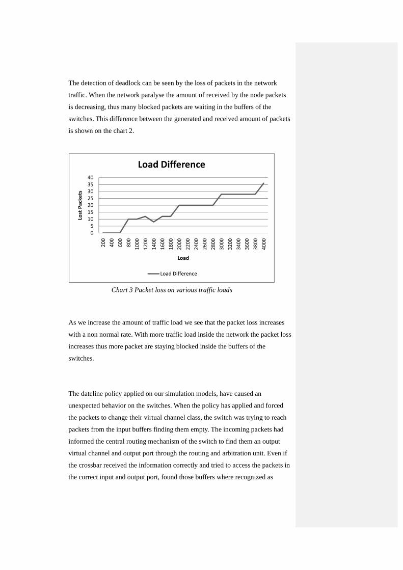
The detection of deadlock can be seen by the loss of packets in the network
traffic. When the network paralyse the amount of received by the node packets
is decreasing, thus many blocked packets are waiting in the buffers of the
switches. This difference between the generated and received amount of packets
is shown on the chart 2.
Chart 3 Packet loss on various traffic loads
As we increase the amount of traffic load we see that the packet loss increases
with a non normal rate. With more traffic load inside the network the packet loss
increases thus more packet are staying blocked inside the buffers of the
switches.
The dateline policy applied on our simulation models, have caused an
unexpected behavior on the switches. When the policy has applied and forced
the packets to change their virtual channel class, the switch was trying to reach
packets from the input buffers finding them empty. The incoming packets had
informed the central routing mechanism of the switch to find them an output
virtual channel and output port through the routing and arbitration unit. Even if
the crossbar received the information correctly and tried to access the packets in
the correct input and output port, found those buffers where recognized as
0
5
10
15
20
25
30
35
40
20
0
40
0
60
0
80
0
10
00
12
00
14
00
16
00
18
00
20
00
22
00
24
00
26
00
28
00
30
00
32
00
34
00
36
00
38
00
40
00
Lost
Pa
cke
ts
Load
Load Difference
Load Difference

113
empty. This problem didn’t give us the opportunity to study in the torus
topology the dateline policy, through the collected simulation results. However,
from the analysis showed at section 6.2.2 we can see how deadlock should be
avoided and network could work normally at loads higher than 1000 Mbps /
node.


115
7 Conclusions
In this work, we have examined the problem of communication deadlock for
interconnection networks. This kind of networks is used in High Performance
Systems and they are a key component of them. Deadlock is one of the problems that
can appear and provokes network paralysation. Deadlock can appear when there is a
circular dependency of some of the resources of the network. In this case, network
buffer are the resources that can produce deadlock depending on the routes the
packets use as determined by the routing algorithm. In order to avoid deadlock, we
use the technique of virtual channels. Using this technique, each physical channel is
split into several virtual channels so several packet flows can use the physical channel
in a multiplexed way over the time. In order to create several virtual channels from a
physical channel, we need to split the buffer associated to this physical channel and
assign each part to a virtual channel.
For conclusions over the phenomenon of deadlock with the use of virtual channels, in
high speed interconnection networks, we can conclude on the below.
Deadlock can be avoided in Mesh topology with the use of DOR algorithm. The
algorithm restricts the packet traffic in specific order on accessing firstly the axis X
and then the axis Y, providing with that way a deadlock free configuration on the
network. DOR is putting an order to the traffic and eliminates the possibility of
dependency cycles between packets and buffers.
The deadlock phenomenon in torus can be avoided with the use of a dateline policy on
its axis. The policy has to be applied on both axis because the torus topology make
use of the wrap around links that form a ring to each one of its axis. The dateline
policy breaks the dependency on the buffers that the packets require, by increasing the
class on the virtual channels through the round robin policy.
Deadlock cannot occur in a topology like fat tree thus the topology is not a
geographically order topology with possibilities on turn between the axis X and Y
thus those axis does not exist. The fat tree manipulates the packet traffic by sending
the packet from the leaf nodes to the root and once more back to the leaf nodes. The
packets follow and order to their traversals over the network without having the
possibility due to network topology to turn and create with that way a cyclic
dependency.
117
8 Bibliography
[1] W. J. Dally and B. Towles, "Principles and practices of interconnection networks".
Amsterdam; San Francisco: Morgan Kaufmann Publishers, 2004, iD: 52902442.
[2] Timothy Mark Pinkston and Jose Duato. “Appendix E of Computer Architecture:
A Quantitative Approach”, 4th Ed., Elsevier Publishers, 2006.
[Online] Available : http://ceng.usc.edu/smart/slides/appendixE.html (July 2009)
[3] J. Duato, S. Yalamanchili, and L. M. Ni, "Interconnection networks. An
Engineering Approach". San Francisco, CA: Morgan Kaufmann, 2003, iD:
52616057.
[4] Chien-Chun Su and Kang G. Shin, "Adaptive Deadlock-Free Routing in
Multicomputers Using Only One Extra Virtual Channel", In International Conference
on Parallel Processing, volume I, Page(s):227 - 231
[5] Smit, Gerard J.M. and Havinga, Paul J.M. and Tibboel, Walter H. (1995) Virtual
lines, a deadlock-free and real-time routing mechanism for ATM networks.
Information Science : Informatics and Computer Science: An International Journal, 85
(1-3). pp. 29-42. ISSN 0020-0255
[6] Dobkin, R. Ginosar, R. Cidon, I. (2007). "QNoC Asynchronous Router with
Dynamic Virtual Channel Allocation". First International Symposium on Networks-
on-Chip, NOCS 2007. Page(s):218 - 218.
[7] Alzeidi N., Khonsari A., Ould-Khaoua M., Mackenzie L., "A new approach to
Field Code Changed
model virtual channels in interconnection networks"(2007) Journal of Computer and
System Sciences, Volume 73 , Issue 8, pp. 1121-1130.
[8] V. S. Adve, M. K. Vernon, "Performance Analysis of Mesh Interconnection
Networks with Deterministic Routing", IEEE Transactions on Parallel and Distributed
Systems, Volume 5 , Issue 3 (March 1994, Pages: 225 - 246
[9] Gerard J. M. Smit, Paul J. M. Havinga, Walter H. Tibboel: "Virtual Lines, a
Deadlock-Free and Real-Time Routing Mechanism for ATM Networks". Information
Sciences—Informatics and Computer Science: An International Journal 85(1-3):
pages 29-42 (1995)
[10] Mullins, R., West, A., and Moore, S. 2004. "Low-Latency Virtual-Channel
Routers for On-Chip Networks". In Proceedings of the 31st Annual international
Symposium on Computer Architecture (München, Germany, June 19 - 23, 2004)
Page(s): 188 - 197