!DE Systems - Copy - Personal homepage...
81
DIFFERENTIAL EQUATIONS Systems of Differential Equations Paul Dawkins
-
Upload
truonghanh -
Category
Documents
-
view
212 -
download
0
Transcript of !DE Systems - Copy - Personal homepage...

DIFFERENTIAL EQUATIONS
Systems of Differential Equations
Paul Dawkins

Differential Equations
© 2007 Paul Dawkins i http://tutorial.math.lamar.edu/terms.aspx
Table of Contents Preface ............................................................................................................................................. 2 Systems of Differential Equations ................................................................................................ 3
Introduction ................................................................................................................................................ 3 Review : Systems of Equations .................................................................................................................. 5 Review : Matrices and Vectors ................................................................................................................ 11 Review : Eigenvalues and Eigenvectors ................................................................................................... 21 Systems of Differential Equations ............................................................................................................ 31 Solutions to Systems ................................................................................................................................ 35 Phase Plane............................................................................................................................................... 37 Real, Distinct Eigenvalues ....................................................................................................................... 42 Complex Eigenvalues ............................................................................................................................... 52 Repeated Eigenvalues .............................................................................................................................. 58 Nonhomogeneous Systems ...................................................................................................................... 65 Laplace Transforms .................................................................................................................................. 69 Modeling .................................................................................................................................................. 71
Differential Equations
© 2007 Paul Dawkins ii http://tutorial.math.lamar.edu/terms.aspx
Preface Here are my online notes for my differential equations course that I teach here at Lamar University. Despite the fact that these are my “class notes”, they should be accessible to anyone wanting to learn how to solve differential equations or needing a refresher on differential equations. I’ve tried to make these notes as self contained as possible and so all the information needed to read through them is either from a Calculus or Algebra class or contained in other sections of the notes. A couple of warnings to my students who may be here to get a copy of what happened on a day that you missed.
1. Because I wanted to make this a fairly complete set of notes for anyone wanting to learn differential equations I have included some material that I do not usually have time to cover in class and because this changes from semester to semester it is not noted here. You will need to find one of your fellow class mates to see if there is something in these notes that wasn’t covered in class.
2. In general I try to work problems in class that are different from my notes. However, with Differential Equation many of the problems are difficult to make up on the spur of the moment and so in this class my class work will follow these notes fairly close as far as worked problems go. With that being said I will, on occasion, work problems off the top of my head when I can to provide more examples than just those in my notes. Also, I often don’t have time in class to work all of the problems in the notes and so you will find that some sections contain problems that weren’t worked in class due to time restrictions.
3. Sometimes questions in class will lead down paths that are not covered here. I try to anticipate as many of the questions as possible in writing these up, but the reality is that I can’t anticipate all the questions. Sometimes a very good question gets asked in class that leads to insights that I’ve not included here. You should always talk to someone who was in class on the day you missed and compare these notes to their notes and see what the differences are.
4. This is somewhat related to the previous three items, but is important enough to merit its own item. THESE NOTES ARE NOT A SUBSTITUTE FOR ATTENDING CLASS!! Using these notes as a substitute for class is liable to get you in trouble. As already noted not everything in these notes is covered in class and often material or insights not in these notes is covered in class.

Differential Equations
© 2007 Paul Dawkins iii http://tutorial.math.lamar.edu/terms.aspx
Systems of Differential Equations
Introduction To this point we’ve only looked as solving single differential equations. However, many “real life” situations are governed by a system of differential equations. Consider the population problems that we looked at back in the modeling section of the first order differential equations chapter. In these problems we looked only at a population of one species, yet the problem also contained some information about predators of the species. We assumed that any predation would be constant in these cases. However, in most cases the level of predation would also be dependent upon the population of the predator. So, to be more realistic we should also have a second differential equation that would give the population of the predators. Also note that the population of the predator would be, in some way, dependent upon the population of the prey as well. In other words, we would need to know something about one population to find the other population. So to find the population of either the prey or the predator we would need to solve a system of at least two differential equations. The next topic of discussion is then how to solve systems of differential equations. However, before doing this we will first need to do a quick review of Linear Algebra. Much of what we will be doing in this chapter will be dependent upon topics from linear algebra. This review is not intended to completely teach you the subject of linear algebra, as that is a topic for a complete class. The quick review is intended to get you familiar enough with some of the basic topics that you will be able to do the work required once we get around to solving systems of differential equations. Here is a brief listing of the topics covered in this chapter.
Review : Systems of Equations – The traditional starting point for a linear algebra class. We will use linear algebra techniques to solve a system of equations.
Review : Matrices and Vectors – A brief introduction to matrices and vectors. We will look at arithmetic involving matrices and vectors, inverse of a matrix, determinant of a matrix, linearly independent vectors and systems of equations revisited. Review : Eigenvalues and Eigenvectors – Finding the eigenvalues and eigenvectors of a matrix. This topic will be key to solving systems of differential equations. Systems of Differential Equations – Here we will look at some of the basics of systems of differential equations. Solutions to Systems – We will take a look at what is involved in solving a system of differential equations. Phase Plane – A brief introduction to the phase plane and phase portraits.

Differential Equations
© 2007 Paul Dawkins 4 http://tutorial.math.lamar.edu/terms.aspx
Real Eigenvalues – Solving systems of differential equations with real eigenvalues. Complex Eigenvalues – Solving systems of differential equations with complex eigenvalues. Repeated Eigenvalues – Solving systems of differential equations with repeated eigenvalues. Nonhomogeneous Systems – Solving nonhomogeneous systems of differential equations using undetermined coefficients and variation of parameters. Laplace Transforms – A very brief look at how Laplace transforms can be used to solve a system of differential equations. Modeling – In this section we’ll take a quick look at some extensions of some of the modeling we did in previous chapters that lead to systems of equations.

Differential Equations
© 2007 Paul Dawkins 5 http://tutorial.math.lamar.edu/terms.aspx
Review : Systems of Equations Because we are going to be working almost exclusively with systems of equations in which the number of unknowns equals the number of equations we will restrict our review to these kinds of systems. All of what we will be doing here can be easily extended to systems with more unknowns than equations or more equations than unknowns if need be. Let’s start with the following system of n equations with the n unknowns, x1, x2,…, xn.
11 1 12 2 1 1
21 1 22 2 2 2
1 1 2 2
n n
n n
n n nn n n
a x a x a x ba x a x a x b
a x a x a x b
+ + + =+ + + =
+ + + =
LLML
(1)
Note that in the subscripts on the coefficients in this system, aij, the i corresponds to the equation that the coefficient is in and the j corresponds to the unknown that is multiplied by the coefficient. To use linear algebra to solve this system we will first write down the augmented matrix for this system. An augmented matrix is really just all the coefficients of the system and the numbers for the right side of the system written in matrix form. Here is the augmented matrix for this system.
11 12 1 1
21 22 2 2
1 2
n
n
n n nn n
a a a ba a a b
a a a b
LL
M M O M ML
To solve this system we will use elementary row operations (which we’ll define these in a bit) to rewrite the augmented matrix in triangular form. The matrix will be in triangular form if all the entries below the main diagonal (the diagonal containing a11, a22, …,ann) are zeroes. Once this is done we can recall that each row in the augmented matrix corresponds to an equation. We will then convert our new augmented matrix back to equations and at this point solving the system will become very easy. Before working an example let’s first define the elementary row operations. There are three of them.
1. Interchange two rows. This is exactly what it says. We will interchange row i with row j. The notation that we’ll use to denote this operation is : i jR R↔
2. Multiply row i by a constant, c. This means that every entry in row i will get multiplied by the constant c. The notation for this operation is : icR
3. Add a multiply of row i to row j. In our heads we will multiply row i by an appropriate constant and then add the results to row j and put the new row back into row j leaving row i in the matrix unchanged. The notation for this operation is : i jcR R+
Differential Equations
© 2007 Paul Dawkins 6 http://tutorial.math.lamar.edu/terms.aspx
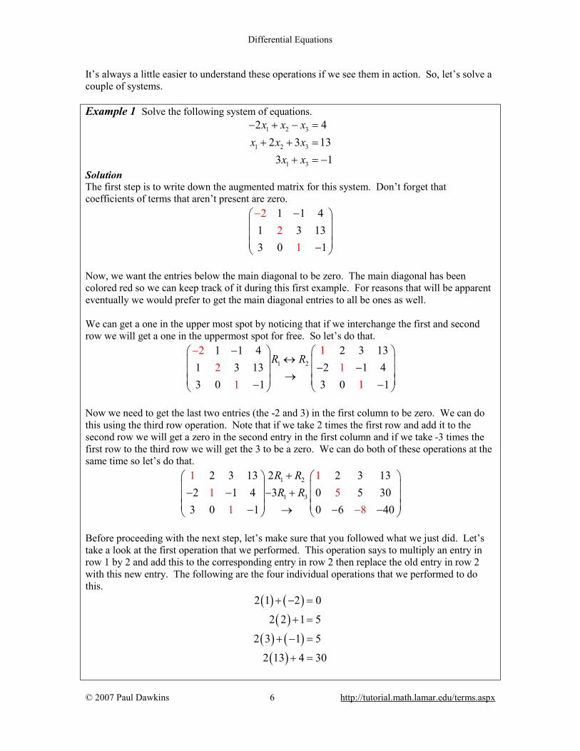
It’s always a little easier to understand these operations if we see them in action. So, let’s solve a couple of systems. Example 1 Solve the following system of equations.
1 2 3
1 2 3
1 3
2 42 3 13
3 1
x x xx x x
x x
− + − =+ + =
+ = −
Solution The first step is to write down the augmented matrix for this system. Don’t forget that coefficients of terms that aren’t present are zero.
2
21
1 1 41 3 133 0 1
− −
−
Now, we want the entries below the main diagonal to be zero. The main diagonal has been colored red so we can keep track of it during this first example. For reasons that will be apparent eventually we would prefer to get the main diagonal entries to all be ones as well. We can get a one in the upper most spot by noticing that if we interchange the first and second row we will get a one in the uppermost spot for free. So let’s do that.
1 2
2 12 1
1 1
1 1 4 2 3 131 3 13 2 1 43 0 1 3 0 1
R R−
↔ − − → − −
−
Now we need to get the last two entries (the -2 and 3) in the first column to be zero. We can do this using the third row operation. Note that if we take 2 times the first row and add it to the second row we will get a zero in the second entry in the first column and if we take -3 times the first row to the third row we will get the 3 to be a zero. We can do both of these operations at the same time so let’s do that.
1 2
1 3
2 3 13 2 2 3 132 1 4 3 0 5 30
3 0 1 0
1 11 5
1 86 40
R RR R
+ − − − + − − −→ −
Before proceeding with the next step, let’s make sure that you followed what we just did. Let’s take a look at the first operation that we performed. This operation says to multiply an entry in row 1 by 2 and add this to the corresponding entry in row 2 then replace the old entry in row 2 with this new entry. The following are the four individual operations that we performed to do this.
( ) ( )( )
( ) ( )( )
2 1 2 0
2 2 1 5
2 3 1 5
2 13 4 30
+ − =
+ =
+ − =
+ =

Differential Equations
© 2007 Paul Dawkins 7 http://tutorial.math.lamar.edu/terms.aspx
Okay, the next step optional, but again is convenient to do. Technically, the 5 in the second column is okay to leave. However, it will make our life easier down the road if it is a 1. We can use the second row operation to take care of this. We can divide the whole row by 5. Doing this gives,
1
25
2 3 13 2 3 130 5 30 0 1 60 6 4
1 15 1
8 80 0 6 40
R → − − − −−−
The next step is to then use the third row operation to make the -6 in the second column into a zero.
2 3
1 11 1
8 2
2 3 13 2 3 136
0 1 6 0 1 60 6 40 0 0 4
R R
+ → − − − − −
Now, officially we are done, but again it’s somewhat convenient to get all ones on the main diagonal so we’ll do one last step.
1
32
2 3 13 2 3 130 1 6 0 1 60 0 4 0
10
1
2 1 2
11
R
− → − −
We can now convert back to equations.
1 2 3
2 3
3
2 3 13 2 3 130 1 6 60 0 2 2
11
1
x x xx x
x
+ + = ⇒ + = =
At this point the solving is quite easy. We get x3 for free and once we get that we can plug this into the second equation and get x2. We can then use the first equation to get x1. Note as well that having 1’s along the main diagonal helped somewhat with this process. The solution to this system of equation is 1 2 31 4 2x x x= − = = The process used in this example is called Gaussian Elimination. Let’s take a look at another example. Example 2 Solve the following system of equations.
Differential Equations
© 2007 Paul Dawkins 8 http://tutorial.math.lamar.edu/terms.aspx
1 2 3
1 2 3
1 2 3
2 3 22 3
2 3 1
x x xx x xx x x
− + = −− + − =
− + =
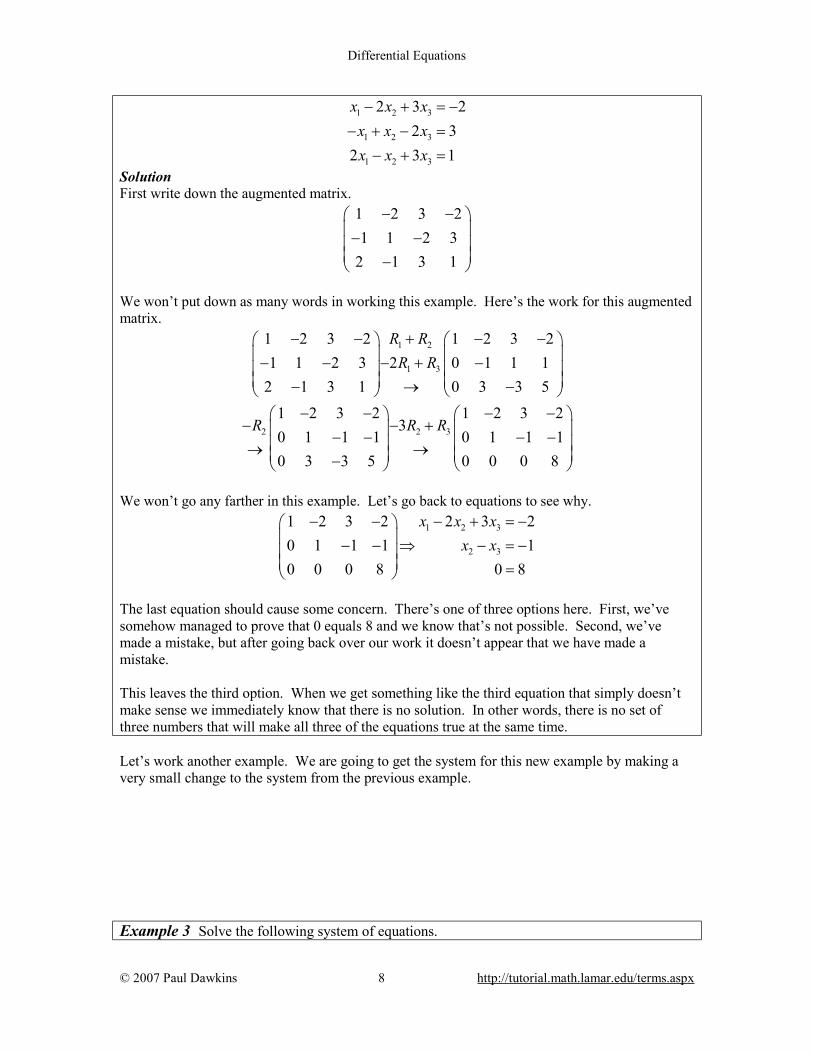
Solution First write down the augmented matrix.
1 2 3 21 1 2 3
2 1 3 1
− − − − −
We won’t put down as many words in working this example. Here’s the work for this augmented matrix.
1 2
1 3
1 2 3 2 1 2 3 21 1 2 3 2 0 1 1 1
2 1 3 1 0 3 3 5
R RR R
− − + − − − − − + − − → −
2 2 3
1 2 3 2 1 2 3 23
0 1 1 1 0 1 1 10 3 3 5 0 0 0 8
R R R− − − −
− − + − − − − → → −
We won’t go any farther in this example. Let’s go back to equations to see why.
1 2 3
2 3
1 2 3 2 2 3 20 1 1 1 10 0 0 8 0 8
x x xx x
− − − + = − − − ⇒ − = − =
The last equation should cause some concern. There’s one of three options here. First, we’ve somehow managed to prove that 0 equals 8 and we know that’s not possible. Second, we’ve made a mistake, but after going back over our work it doesn’t appear that we have made a mistake. This leaves the third option. When we get something like the third equation that simply doesn’t make sense we immediately know that there is no solution. In other words, there is no set of three numbers that will make all three of the equations true at the same time. Let’s work another example. We are going to get the system for this new example by making a very small change to the system from the previous example. Example 3 Solve the following system of equations.
Differential Equations
© 2007 Paul Dawkins 9 http://tutorial.math.lamar.edu/terms.aspx
1 2 3
1 2 3
1 2 3
2 3 22 3
2 3 7
x x xx x xx x x
− + = −− + − =
− + = −
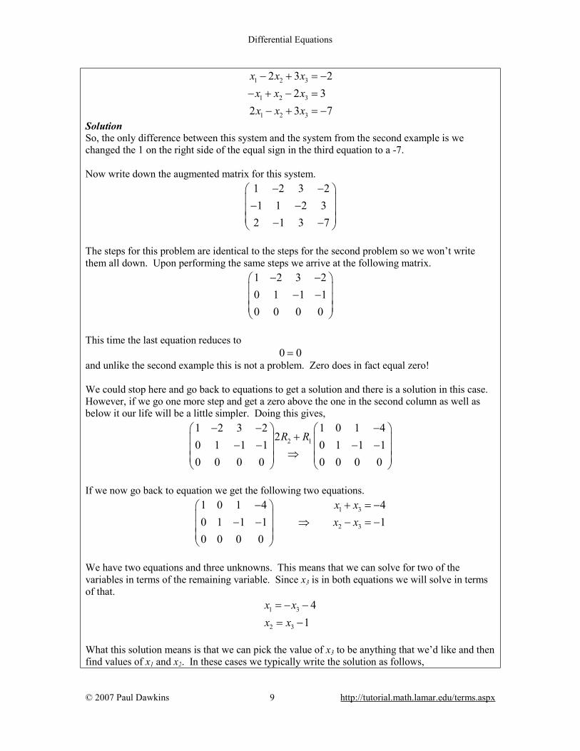
Solution So, the only difference between this system and the system from the second example is we changed the 1 on the right side of the equal sign in the third equation to a -7. Now write down the augmented matrix for this system.
1 2 3 21 1 2 3
2 1 3 7
− − − − − −
The steps for this problem are identical to the steps for the second problem so we won’t write them all down. Upon performing the same steps we arrive at the following matrix.
1 2 3 20 1 1 10 0 0 0
− − − −
This time the last equation reduces to 0 0= and unlike the second example this is not a problem. Zero does in fact equal zero! We could stop here and go back to equations to get a solution and there is a solution in this case. However, if we go one more step and get a zero above the one in the second column as well as below it our life will be a little simpler. Doing this gives,
2 1
1 2 3 2 1 0 1 42
0 1 1 1 0 1 1 10 0 0 0 0 0 0 0
R R− − −
+ − − − − ⇒
If we now go back to equation we get the following two equations.
1 3
2 3
1 0 1 4 40 1 1 1 10 0 0 0
x xx x
− + = − − − ⇒ − = −
We have two equations and three unknowns. This means that we can solve for two of the variables in terms of the remaining variable. Since x3 is in both equations we will solve in terms of that.
1 3
2 3
41
x xx x
= − −
= −
What this solution means is that we can pick the value of x3 to be anything that we’d like and then find values of x1 and x2. In these cases we typically write the solution as follows,
Differential Equations
© 2007 Paul Dawkins 10 http://tutorial.math.lamar.edu/terms.aspx
1
2
3
41 any real number
x tx t tx t
= − −= − ==
In this way we get an infinite number of solutions, one for each and every value of t. These three examples lead us to a nice fact about systems of equations. Fact Given a system of equations, (1), we will have one of the three possibilities for the number of solutions.
1. No solution. 2. Exactly one solution. 3. Infinitely many solutions.
Before moving on to the next section we need to take a look at one more situation. The system of equations in (1) is called a nonhomogeneous system if at least one of the bi’s is not zero. If however all of the bi’s are zero we call the system homogeneous and the system will be,
11 1 12 2 1
21 1 22 2 2
1 1 2 2
00
0
n n
n n
n n nn n
a x a x a xa x a x a x
a x a x a x
+ + + =+ + + =
+ + + =
LLML
(2)
Now, notice that in the homogeneous case we are guaranteed to have the following solution. 1 2 0nx x x= = = =L This solution is often called the trivial solution. For homogeneous systems the fact above can be modified to the following. Fact Given a homogeneous system of equations, (2), we will have one of the two possibilities for the number of solutions.
1. Exactly one solution, the trivial solution 2. Infinitely many non-zero solutions in addition to the trivial solution.
In the second possibility we can say non-zero solution because if there are going to be infinitely many solutions and we know that one of them is the trivial solution then all the rest must have at least one of the xi’s be non-zero and hence we get a non-zero solution.

Differential Equations
© 2007 Paul Dawkins 11 http://tutorial.math.lamar.edu/terms.aspx
Review : Matrices and Vectors This section is intended to be a catch all for many of the basic concepts that are used occasionally in working with systems of differential equations. There will not be a lot of details in this section, nor will we be working large numbers of examples. Also, in many cases we will not be looking at the general case since we won’t need the general cases in our differential equations work. Let’s start with some of the basic notation for matrices. An n x m (this is often called the size or dimension of the matrix) matrix is a matrix with n rows and m columns and the entry in the ith row and jth column is denoted by aij. A short hand method of writing a general n x m matrix is the following.
( )11 12 1
21 22 2
x
1 2 x
m
mij n m
n n nm n m
a a aa a a
A a
a a a
= =
LL
M M ML
The size or dimension of a matrix is subscripted as shown if required. If it’s not required or clear from the problem the subscripted size is often dropped from the matrix. Special Matrices There are a few “special” matrices out there that we may use on occasion. The first special matrix is the square matrix. A square matrix is any matrix whose size (or dimension) is n x n. In other words it has the same number of rows as columns. In a square matrix the diagonal that starts in the upper left and ends in the lower right is often called the main diagonal. The next two special matrices that we want to look at are the zero matrix and the identity matrix. The zero matrix, denoted 0n x m , is a matrix all of whose entries are zeroes. The identity matrix is a square n x n matrix, denoted In, whose main diagonals are all 1’s and all the other elements are zero. Here are the general zero and identity matrices.
x
x x
1 0 00 0 0
0 1 00
0 0 00 0 1
n m n
n mn n
I
= =
LL
LM M M
M M O ML
L
In matrix arithmetic these two matrices will act in matrix work like zero and one act in the real number system. The last two special matrices that we’ll look at here are the column matrix and the row matrix. These are matrices that consist of a single column or a single row. In general they are,
( )
1
21 2 1 x
x 1
m m
n n
xx
x y y y y
x
= =
LM
We will often refer to these as vectors.

Differential Equations
© 2007 Paul Dawkins 12 http://tutorial.math.lamar.edu/terms.aspx
Arithmetic We next need to take a look at arithmetic involving matrices. We’ll start with addition and subtraction of two matrices. So, suppose that we have two n x m matrices, A and B. The sum (or difference) of these two matrices is then, ( ) ( ) ( ) x x x x x n m n m ij ij ij ijn m n m n m
A B a b a b± = ± = ± The sum or difference of two matrices of the same size is a new matrix of identical size whose entries are the sum or difference of the corresponding entries from the original two matrices. Note that we can’t add or subtract entries with different sizes. Next, let’s look at scalar multiplication. In scalar multiplication we are going to multiply a matrix A by a constant (sometimes called a scalar) α. In this case we get a new matrix whose entries have all been multiplied by the constant, α. ( ) ( ) x x x n m ij ijn m n m
A a aα α α= = Example 1 Given the following two matrices,
3 2 4 19 1 0 5
A B− −
= = − −
compute A-5B. Solution There isn’t much to do here other than the work.
3 2 4 15 5
9 1 0 5
3 2 20 59 1 0 25
23 79 26
A B− −
− = − − − − −
= − − − −
= −
We first multiplied all the entries of B by 5 then subtracted corresponding entries to get the entries in the new matrix. The final matrix operation that we’ll take a look at is matrix multiplication. Here we will start with two matrices, An x p and Bp x m . Note that A must have the same number of columns as B has rows. If this isn’t true then we can’t perform the multiplication. If it is true then we can perform the following multiplication. ( ) x x x n p p m ij n m
A B c= The new matrix will have size n x m and the entry in the ith row and jth column, cij, is found by multiplying row i of matrix A by column j of matrix B. This doesn’t always make sense in words so let’s look at an example.
Differential Equations
© 2007 Paul Dawkins 13 http://tutorial.math.lamar.edu/terms.aspx
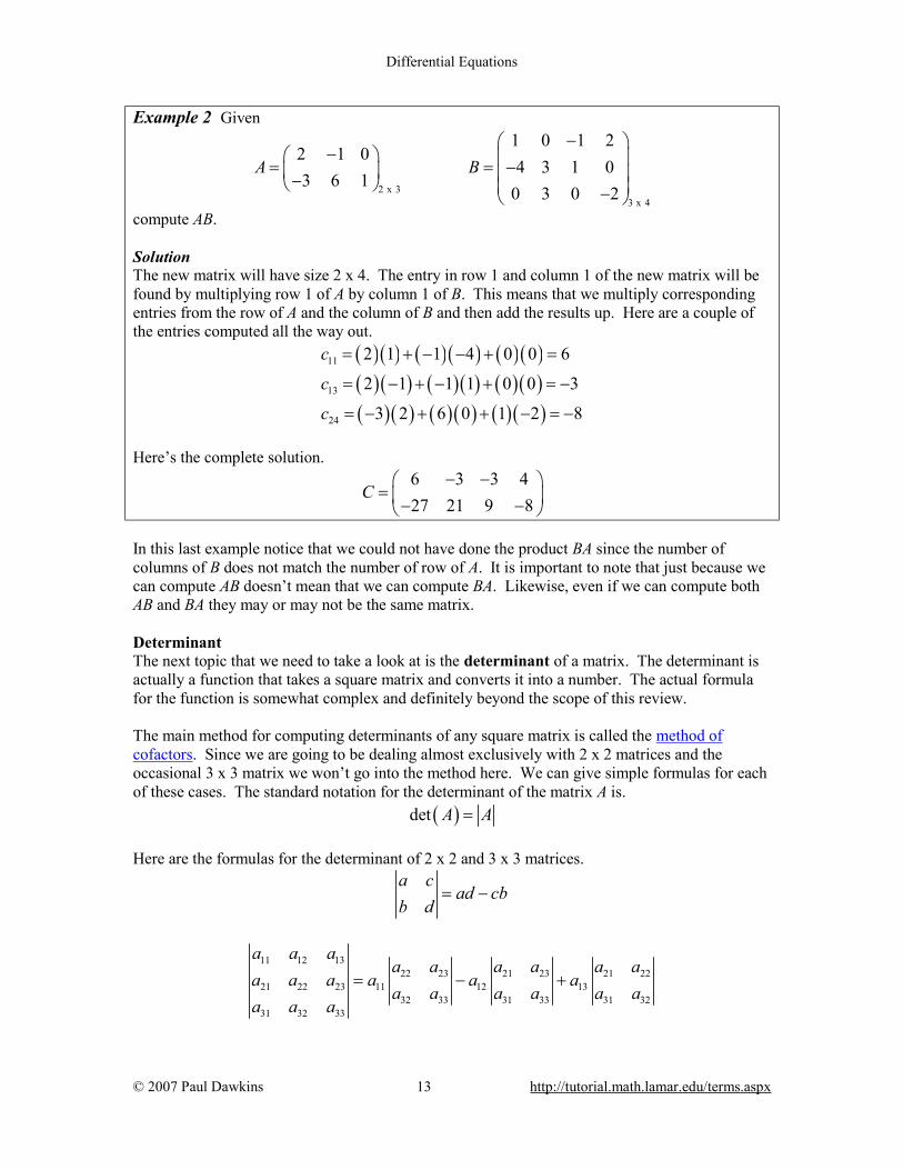
Example 2 Given
2 x 3
3 x 4
1 0 1 22 1 0
4 3 1 03 6 1
0 3 0 2A B
− − = = − − −
compute AB. Solution The new matrix will have size 2 x 4. The entry in row 1 and column 1 of the new matrix will be found by multiplying row 1 of A by column 1 of B. This means that we multiply corresponding entries from the row of A and the column of B and then add the results up. Here are a couple of the entries computed all the way out.
( )( ) ( )( ) ( ) ( )( ) ( ) ( )( ) ( )( )( )( ) ( ) ( ) ( ) ( )
11
13
24
2 1 1 4 0 0 6
2 1 1 1 0 0 3
3 2 6 0 1 2 8
c
c
c
= + − − + =
= − + − + = −
= − + + − = −
Here’s the complete solution.
6 3 3 427 21 9 8
C− −
= − −
In this last example notice that we could not have done the product BA since the number of columns of B does not match the number of row of A. It is important to note that just because we can compute AB doesn’t mean that we can compute BA. Likewise, even if we can compute both AB and BA they may or may not be the same matrix. Determinant The next topic that we need to take a look at is the determinant of a matrix. The determinant is actually a function that takes a square matrix and converts it into a number. The actual formula for the function is somewhat complex and definitely beyond the scope of this review. The main method for computing determinants of any square matrix is called the method of cofactors. Since we are going to be dealing almost exclusively with 2 x 2 matrices and the occasional 3 x 3 matrix we won’t go into the method here. We can give simple formulas for each of these cases. The standard notation for the determinant of the matrix A is. ( )det A A= Here are the formulas for the determinant of 2 x 2 and 3 x 3 matrices.
a c
ad cbb d
= −
11 12 13
22 23 21 23 21 2221 22 23 11 12 13
32 33 31 33 31 3231 32 33
a a aa a a a a a
a a a a a aa a a a a a
a a a= − +
Differential Equations
© 2007 Paul Dawkins 14 http://tutorial.math.lamar.edu/terms.aspx
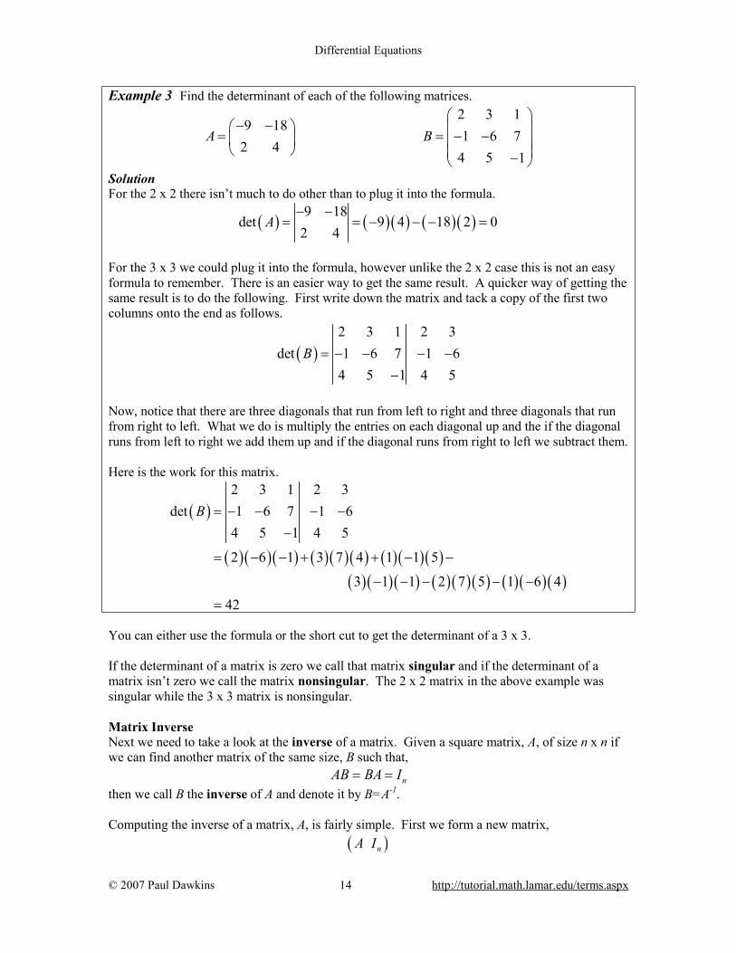
Example 3 Find the determinant of each of the following matrices.
2 3 1
9 181 6 7
2 44 5 1
A B
− − = = − − −
Solution For the 2 x 2 there isn’t much to do other than to plug it into the formula.
( ) ( ) ( ) ( )( )9 18det 9 4 18 2 0
2 4A
− −= = − − − =
For the 3 x 3 we could plug it into the formula, however unlike the 2 x 2 case this is not an easy formula to remember. There is an easier way to get the same result. A quicker way of getting the same result is to do the following. First write down the matrix and tack a copy of the first two columns onto the end as follows.
( )2 3 1 2 3
det 1 6 7 1 64 5 1 4 5
B = − − − −−
Now, notice that there are three diagonals that run from left to right and three diagonals that run from right to left. What we do is multiply the entries on each diagonal up and the if the diagonal runs from left to right we add them up and if the diagonal runs from right to left we subtract them. Here is the work for this matrix.
( )
( )( )( ) ( )( )( ) ( )( )( )( ) ( ) ( ) ( ) ( ) ( ) ( )( )( )
2 3 1 2 3det 1 6 7 1 6
4 5 1 4 5
2 6 1 3 7 4 1 1 5
3 1 1 2 7 5 1 6 442
B = − − − −−
= − − + + − −
− − − − −
=
You can either use the formula or the short cut to get the determinant of a 3 x 3. If the determinant of a matrix is zero we call that matrix singular and if the determinant of a matrix isn’t zero we call the matrix nonsingular. The 2 x 2 matrix in the above example was singular while the 3 x 3 matrix is nonsingular. Matrix Inverse Next we need to take a look at the inverse of a matrix. Given a square matrix, A, of size n x n if we can find another matrix of the same size, B such that, nAB BA I= = then we call B the inverse of A and denote it by B=A-1. Computing the inverse of a matrix, A, is fairly simple. First we form a new matrix, ( )nA I
Differential Equations
© 2007 Paul Dawkins 15 http://tutorial.math.lamar.edu/terms.aspx
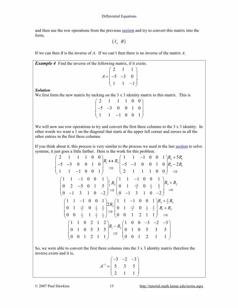
and then use the row operations from the previous section and try to convert this matrix into the form, ( )nI B If we can then B is the inverse of A. If we can’t then there is no inverse of the matrix A. Example 4 Find the inverse of the following matrix, if it exists.
2 1 15 3 0
1 1 1A
= − − −
Solution We first form the new matrix by tacking on the 3 x 3 identity matrix to this matrix. This is
2 1 1 1 0 05 3 0 0 1 0
1 1 1 0 0 1
− − −
We will now use row operations to try and convert the first three columns to the 3 x 3 identity. In other words we want a 1 on the diagonal that starts at the upper left corner and zeroes in all the other entries in the first three columns. If you think about it, this process is very similar to the process we used in the last section to solve systems, it just goes a little farther. Here is the work for this problem.
2 1
1 33 1
2 1 1 1 0 0 1 1 1 0 0 1 55 3 0 0 1 0 5 3 0 0 1 0 2
1 1 1 0 0 1 2 1 1 1 0 0
R RR R
R R− +
↔ − − − − − ⇒ − ⇒
1
3 22 5 5122 2 2
1 1 1 0 0 1 1 1 1 0 0 10 2 5 0 1 5 0 1 00 1 3 1 0 2 0 1 3 1 0 2
R RR −
− − + − ⇒⇒ − − − −
52 32
35 5 5 51 11 32 2 2 2 2 2
1 1 12 2 2
1 1 1 0 0 1 1 1 1 0 0 12
0 1 0 0 1 00 0 1 0 0 1 2 1 1
R RR
R R− −
− − + + ⇒ ⇒
1 2
1 1 0 2 1 2 1 0 0 3 2 30 1 0 5 3 5 0 1 0 5 3 50 0 1 2 1 1 0 0 1 2 1 1
R R− − −
− ⇒
So, we were able to convert the first three columns into the 3 x 3 identity matrix therefore the inverse exists and it is,
1
3 2 35 3 52 1 1
A−
− − − =

Differential Equations
© 2007 Paul Dawkins 16 http://tutorial.math.lamar.edu/terms.aspx
So, there was an example in which the inverse did exist. Let’s take a look at an example in which the inverse doesn’t exist. Example 5 Find the inverse of the following matrix, provided it exists.
1 32 6
B−
= −
Solution In this case we will tack on the 2 x 2 identity to get the new matrix and then try to convert the first two columns to the 2 x 2 identity matrix.
1 21 3 1 0 2 1 3 1 02 6 0 1 0 0 2 1
R R− + − − ⇒
And we don’t need to go any farther. In order for the 2 x 2 identity to be in the first two columns we must have a 1 in the second entry of the second column and a 0 in the second entry of the first column. However, there is no way to get a 1 in the second entry of the second column that will keep a 0 in the second entry in the first column. Therefore, we can’t get the 2 x 2 identity in the first two columns and hence the inverse of B doesn’t exist. We will leave off this discussion of inverses with the following fact. Fact Given a square matrix A.
1. If A is nonsingular then A-1 will exist. 2. If A is singular then A-1 will NOT exist.
I’ll leave it to you to verify this fact for the previous two examples. Systems of Equations Revisited We need to do a quick revisit of systems of equations. Let’s start with a general system of equations.
11 1 12 2 1 1
21 1 22 2 2 2
1 1 2 2
n n
n n
n n nn n n
a x a x a x ba x a x a x b
a x a x a x b
+ + + =+ + + =
+ + + =
LLML
(1)
Now, covert each side into a vector to get,
11 1 12 2 1 1
21 1 22 2 2 2
1 1 2 2
n n
n n
n n nn n n
a x a x a x ba x a x a x b
a x a x a x b
+ + + + + + =
+ + +
LL
M ML
The left side of this equation can be thought of as a matrix multiplication.

Differential Equations
© 2007 Paul Dawkins 17 http://tutorial.math.lamar.edu/terms.aspx
11 12 1 1 1
21 22 2 2 2
1 2
n
n
n n nn n n
a a a x ba a a x b
a a a x b
=
LL
M M O M M ML
Simplifying up the notation a little gives, Ax b=
rr (2) where, xr is a vector whose components are the unknowns in the original system of equations. We call (2) the matrix form of the system of equations (1) and solving (2) is equivalent to solving (1). The solving process is identical. The augmented matrix for (2) is ( )A b
r
Once we have the augmented matrix we proceed as we did with a system that hasn’t been wrote in matrix form. We also have the following fact about solutions to (2). Fact Given the system of equation (2) we have one of the following three possibilities for solutions.
1. There will be no solutions. 2. There will be exactly one solution. 3. There will be infinitely many solutions.
In fact we can go a little farther now. Since we are assuming that we’ve got the same number of equations as unknowns the matrix A in (2) is a square matrix and so we can compute its determinant. This gives the following fact. Fact Given the system of equations in (2) we have the following.
1. If A is nonsingular then there will be exactly one solution to the system. 2. If A is singular then there will either be no solution or infinitely many solutions to the
system. The matrix form of a homogeneous system is 0Ax =
rr (3) where 0
r is the vector of all zeroes. In the homogeneous system we are guaranteed to have a
solution, 0x =rr
. The fact above for homogeneous systems is then, Fact Given the homogeneous system (3) we have the following.
1. If A is nonsingular then the only solution will be 0x =rr
. 2. If A is singular then there will be infinitely many nonzero solutions to the system.
Linear Independence/Linear Dependence This is not the first time that we’ve seen this topic. We also saw linear independence and linear dependence back when we were looking at second order differential equations. In that section we

Differential Equations
© 2007 Paul Dawkins 18 http://tutorial.math.lamar.edu/terms.aspx
were dealing with functions, but the concept is essentially the same here. If we start with n vectors, 1 2, , , nx x xr r r… If we can find constants, c1,c2,…,cn with at least two nonzero such that 1 1 2 2 0n nc x c x c x+ + + =
rr r r… (4) then we call the vectors linearly dependent. If the only constants that work in (4) are c1=0, c2=0, …, cn=0 then we call the vectors linearly independent. If we further make the assumption that each of the n vectors has n components, i.e. each of the vectors look like,
1
2
n
xx
x
x
=
rM
we can get a very simple test for linear independence and linear dependence. Note that this does not have to be the case, but in all of our work we will be working with n vectors each of which has n components. Fact Given the n vectors each with n components,
1 2, , , nx x xr r r… form the matrix,
( )1 2 nX x x x=r r rL
So, the matrix X is a matrix whose ith column is the ith vector, ixr . Then, 1. If X is nonsingular (i.e. det(X) is not zero) then the n vectors are linearly independent, and 2. if X is singular (i.e. det(X) = 0) then the n vectors are linearly dependent and the constants
that make (4) true can be found by solving the system 0X c =rr
where cr is a vector containing the constants in (4). Example 6 Determine if the following set of vectors are linearly independent or linearly dependent. If they are linearly dependent find the relationship between them.
(1) (2) (3)
1 2 63 , 1 , 2
5 4 1x x x
− = − = = −
r r r
Solution So, the first thing to do is to form X and compute its determinant.
( )1 2 63 1 2 det 79
5 4 1X X
− = − − ⇒ = −
This matrix is non singular and so the vectors are linearly independent.
Differential Equations
© 2007 Paul Dawkins 19 http://tutorial.math.lamar.edu/terms.aspx
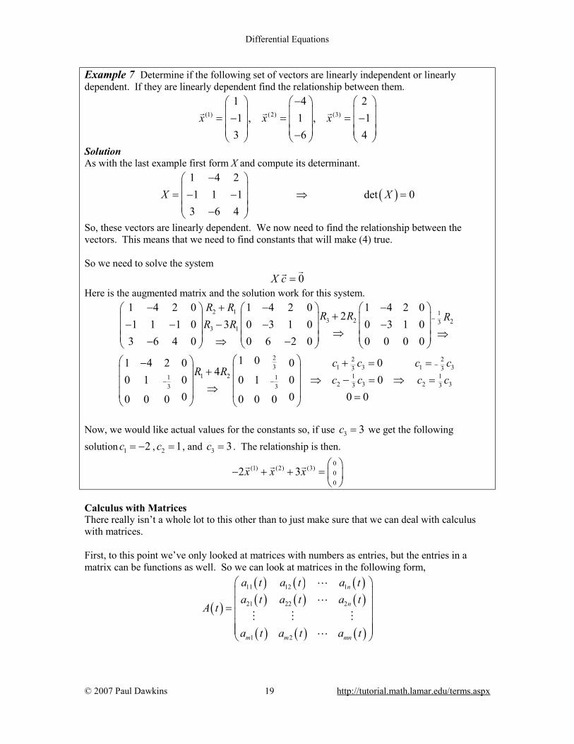
Example 7 Determine if the following set of vectors are linearly independent or linearly dependent. If they are linearly dependent find the relationship between them.
(1) (2) (3)
1 4 21 , 1 , 1
3 6 4x x x
− = − = = − −
r r r
Solution As with the last example first form X and compute its determinant.
( )1 4 21 1 1 det 0
3 6 4X X
− = − − ⇒ = −
So, these vectors are linearly dependent. We now need to find the relationship between the vectors. This means that we need to find constants that will make (4) true. So we need to solve the system 0X c =
rr Here is the augmented matrix and the solution work for this system.
2 1 13 2 23
3 1
1 4 2 0 1 4 2 0 1 4 2 02
1 1 1 0 3 0 3 1 0 0 3 1 03 6 4 0 0 6 2 0 0 0 0 0
R RR R R
R R−
− + − − + − − − − − ⇒ ⇒ − ⇒ −
2 2 23 1 3 1 33 3
1 2 1 11 12 3 2 33 33 3
1 01 4 2 0 0 04
0 1 0 0 1 0 00 0 0 00 0 0 0 0 0
c c c cR R
c c c c−
− −
− + = = +
⇒ − = ⇒ = ⇒ =
Now, we would like actual values for the constants so, if use 3 3c = we get the following solution 1 2c = − , 2 1c = , and 3 3c = . The relationship is then.
0
(1) (2) (3)00
2 3x x x − + + =
r r r
Calculus with Matrices There really isn’t a whole lot to this other than to just make sure that we can deal with calculus with matrices. First, to this point we’ve only looked at matrices with numbers as entries, but the entries in a matrix can be functions as well. So we can look at matrices in the following form,
( )
( ) ( ) ( )( ) ( ) ( )
( ) ( ) ( )
11 12 1
21 22 2
1 2
n
n
m m mn
a t a t a ta t a t a t
A t
a t a t a t
=
LL
M M ML
Differential Equations
© 2007 Paul Dawkins 20 http://tutorial.math.lamar.edu/terms.aspx
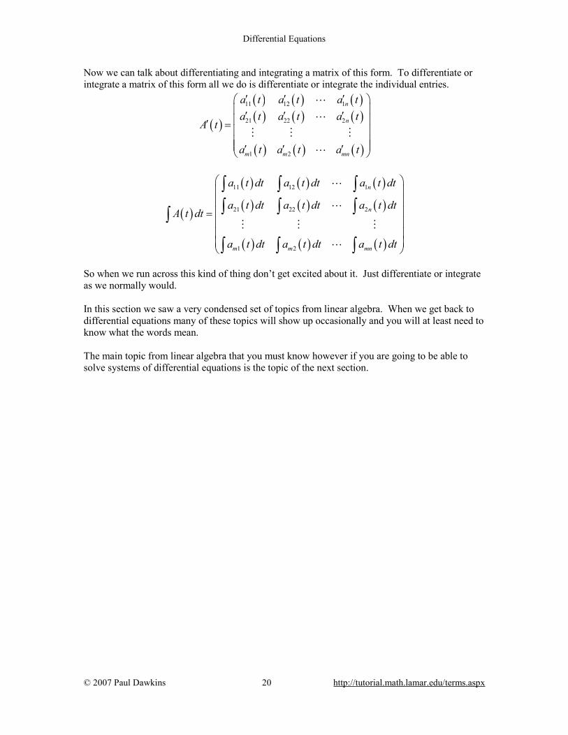
Now we can talk about differentiating and integrating a matrix of this form. To differentiate or integrate a matrix of this form all we do is differentiate or integrate the individual entries.
( )
( ) ( ) ( )( ) ( ) ( )
( ) ( ) ( )
11 12 1
21 22 2
1 2
n
n
m m mn
a t a t a ta t a t a t
A t
a t a t a t
′ ′ ′ ′ ′ ′ ′ = ′ ′ ′
LL
M M ML
( )
( ) ( ) ( )( ) ( ) ( )
( ) ( ) ( )
11 12 1
21 22 2
1 2
n
n
m m mn
a t dt a t dt a t dt
a t dt a t dt a t dtA t dt
a t dt a t dt a t dt
=
∫ ∫ ∫∫ ∫ ∫∫
∫ ∫ ∫
L
L
M M M
L
So when we run across this kind of thing don’t get excited about it. Just differentiate or integrate as we normally would. In this section we saw a very condensed set of topics from linear algebra. When we get back to differential equations many of these topics will show up occasionally and you will at least need to know what the words mean. The main topic from linear algebra that you must know however if you are going to be able to solve systems of differential equations is the topic of the next section.

Differential Equations
© 2007 Paul Dawkins 21 http://tutorial.math.lamar.edu/terms.aspx
Review : Eigenvalues and Eigenvectors If you get nothing out of this quick review of linear algebra you must get this section. Without this section you will not be able to do any of the differential equations work that is in this chapter. So let’s start with the following. If we multiply an n x n matrix by an n x 1 vector we will get a new n x 1 vector back. In other words, A yη =
r r What we want to know is if it is possible for the following to happen. Instead of just getting a brand new vector out of the multiplication is it possible instead to get the following, Aη λη=
r r (1) In other words is it possible, at least for certain λ andη
r, to have matrix multiplication be the
same as just multiplying the vector by a constant? Of course, we probably wouldn’t be talking about this if the answer was no. So, it is possible for this to happen, however, it won’t happen for just any value of λ orη
r. If we do happen to have a λ andη
r for which this works (and they will
always come in pairs) then we call λ an eigenvalue of A and ηr
an eigenvector of A. So, how do we go about find the eigenvalues and eigenvectors for a matrix? Well first notice that that if 0η =
rr then (1) is going to be true for any value of λ and so we are going to make the
assumption that 0η ≠rr
. With that out of the way let’s rewrite (1) a little.
( )
0
0
0n
n
A
A I
A I
η λη
η λ η
λ η
− =
− =
− =
rr rrr rrr
Notice that before we factored out theη
r we added in the appropriately sized identity matrix.
This is equivalent to multiplying things by a one and so doesn’t change the value of anything. We needed to do this because without it we would have had the difference of a matrix, A, and a constant, λ, and this can’t be done. We now have the difference of two matrices of the same size which can be done. So, with this rewrite we see that ( ) 0nA Iλ η− =
rr (2) is equivalent to (1). In order to find the eigenvectors for a matrix we will need to solve a homogeneous system. Recall the fact from the previous section that we know that we will either have exactly one solution ( 0η =
rr) or we will have infinitely many nonzero solutions. Since
we’ve already said that don’t want 0η =rr
this means that we want the second case. Knowing this will allow us to find the eigenvalues for a matrix. Recall from this fact that we will get the second case only if the matrix in the system is singular. Therefore we will need to determine the values of λ for which we get, ( )det 0A Iλ− =

Differential Equations
© 2007 Paul Dawkins 22 http://tutorial.math.lamar.edu/terms.aspx
Once we have the eigenvalues we can then go back and determine the eigenvectors for each eigenvalue. Let’s take a look at a couple of quick facts about eigenvalues and eigenvectors. Fact If A is an n x n matrix then ( )det 0A Iλ− = is an nth degree polynomial. This polynomial is called the characteristic polynomial. To find eigenvalues of a matrix all we need to do is solve a polynomial. That’s generally not too bad provided we keep n small. Likewise this fact also tells us that for an n x n matrix, A, we will have n eigenvalues if we include all repeated eigenvalues. Fact If 1 2, , , nλ λ λ… is the complete list of eigenvalues for A (including all repeated eigenvalues) then,
1. If λ occurs only once in the list then we call λ simple. 2. If λ occurs k>1 times in the list then we say that λ has multiplicity k. 3. If 1 2, , , nλ λ λ… ( k n≤ ) are the simple eigenvalues in the list with corresponding
eigenvectors ( )1ηr
, ( )2ηr
, …, ( )kηr
then the eigenvectors are all linearly independent. 4. If λ is an eigenvalue of k > 1 then λ will have anywhere from 1 to k linearly
independent eigenvectors. The usefulness of these facts will become apparent when we get back into differential equations since in that work we will want linearly independent solutions. Let’s work a couple of examples now to see how we actually go about finding eigenvalues and eigenvectors. Example 1 Find the eigenvalues and eigenvectors of the following matrix.
2 71 6
A = − −
Solution The first thing that we need to do is find the eigenvalues. That means we need the following matrix,
2 7 1 0 2 71 6 0 1 1 6
A Iλ
λ λλ
− − = − = − − − − −
In particular we need to determine where the determinant of this matrix is zero. ( ) ( )( ) ( )( )2det 2 6 7 4 5 5 1A Iλ λ λ λ λ λ λ− = − − − + = + − = + − So, it looks like we will have two simple eigenvalues for this matrix, 1 5λ = − and 2 1λ = . We will now need to find the eigenvectors for each of these. Also note that according to the fact above, the two eigenvectors should be linearly independent. To find the eigenvectors we simply plug in each eigenvalue into (2) and solve. So, let’s do that.

Differential Equations
© 2007 Paul Dawkins 23 http://tutorial.math.lamar.edu/terms.aspx
1 5λ = − :
In this case we need to solve the following system.
7 7 01 1 0
η
= − −
r
Recall that officially to solve this system we use the following augmented matrix.
1
1 277 7 0 7 7 01 1 0 0 0 0
R R+ − − ⇒
Upon reducing down we see that we get a single equation 1 2 1 27 7 0η η η η+ = ⇒ = − that will yield an infinite number of solutions. This is expected behavior. Recall that we picked the eigenvalues so that the matrix would be singular and so we would get infinitely many solutions. Notice as well that we could have identified this from the original system. This won’t always be the case, but in the 2 x 2 case we can see from the system that one row will be a multiple of the other and so we will get infinite solutions. From this point on we won’t be actually solving systems in these cases. We will just go straight to the equation and we can use either of the two rows for this equation. Now, let’s get back to the eigenvector, since that is what we were after. In general then the eigenvector will be any vector that satisfies the following,
1 22
2 2
, 0η η
η ηη η
− = = ≠
r
To get this we used the solution to the equation that we found above. We really don’t want a general eigenvector however so we will pick a value for 2η to get a
specific eigenvector. We can choose anything (except 2 0η = ), so pick something that will make the eigenvector “nice”. Note as well that since we’ve already assumed that the eigenvector is not zero we must choose a value that will not give us zero, which is why we want to avoid 2 0η = in this case. Here’s the eigenvector for this eigenvalue.
( )12
1, using 1
1η η
− = =
r
Now we get to do this all over again for the second eigenvalue.
2 1λ = : We’ll do much less work with this part than we did with the previous part. We will need to solve the following system.
1 7 01 7 0
η
= − −
r

Differential Equations
© 2007 Paul Dawkins 24 http://tutorial.math.lamar.edu/terms.aspx
Clearly both rows are multiples of each other and so we will get infinitely many solutions. We can choose to work with either row. We’ll run with the first because to avoid having too many minus signs floating around. Doing this gives us, 1 2 1 27 0 7η η η η+ = = − Note that we can solve this for either of the two variables. However, with an eye towards working with these later on let’s try to avoid as many fractions as possible. The eigenvector is then,
1 22
2 2
7, 0
η ηη η
η η−
= = ≠
r
( )22
7, using 1
1η η
− = =
r
Summarizing we have,
( )
( )
11
12
15
1
71
1
λ η
λ η
− = − =
−
= =
r
r
Note that the two eigenvectors are linearly independent as predicted. Example 2 Find the eigenvalues and eigenvectors of the following matrix.
4 19 3
1 1A
− = −
Solution This matrix has fractions in it. That’s life so don’t get excited about it. First we need the eigenvalues.
( )
( )
4 19 3
2
2
1,2
1 1det
1 413 9
2 13 91 13 3
A Iλ
λλ
λ λ
λ λ
λ λ
− −− =
− −
= − − − +
= − +
= − ⇒ =
So, it looks like we’ve got an eigenvalue of multiplicity 2 here. Remember that the power on the term will be the multiplicity. Now, let’s find the eigenvector(s). This one is going to be a little different from the first example. There is only one eigenvalue so let’s do the work for that one. We will need to solve the following system,
Differential Equations
© 2007 Paul Dawkins 25 http://tutorial.math.lamar.edu/terms.aspx
2
131 24 2
29 3
1 0 30 2
R Rηη
− = ⇒ = −
So, the rows are multiples of each other. We’ll work with the first equation in this example to find the eigenvector.
1 2 2 12 203 3
η η η η− = =
Recall in the last example we decided that we wanted to make these as “nice” as possible and so should avoid fractions if we can. Sometimes, as in this case, we simply can’t so we’ll have to deal with it. In this case the eigenvector will be,
1112
12 3
, 0ηη
η ηηη
= = ≠
r
( )11
3, 3
2η η
= =
r
Note that by careful choice of the variable in this case we were able to get rid of the fraction that we had. This is something that in general doesn’t much matter if we do or not. However, when we get back to differential equations it will be easier on us if we don’t have any fractions so we will usually try to eliminate them at this step. Also in this case we are only going to get a single (linearly independent) eigenvector. We can get other eigenvectors, by choosing different values of 1η . However, each of these will be linearly dependent with the first eigenvector. If you’re not convinced of this try it. Pick some values for
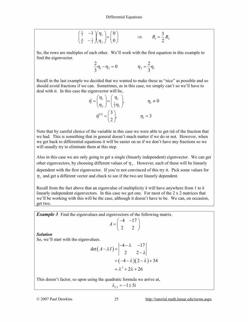
1η and get a different vector and check to see if the two are linearly dependent. Recall from the fact above that an eigenvalue of multiplicity k will have anywhere from 1 to k linearly independent eigenvectors. In this case we got one. For most of the 2 x 2 matrices that we’ll be working with this will be the case, although it doesn’t have to be. We can, on occasion, get two. Example 3 Find the eigenvalues and eigenvectors of the following matrix.
4 17
2 2A
− − =
Solution So, we’ll start with the eigenvalues.
( )
( ) ( )2
4 17det
2 2
4 2 34
2 26
A Iλ
λλ
λ λ
λ λ
− − −− =
−
= − − − +
= + +
This doesn’t factor, so upon using the quadratic formula we arrive at, 1,2 1 5iλ = − ±

Differential Equations
© 2007 Paul Dawkins 26 http://tutorial.math.lamar.edu/terms.aspx
In this case we get complex eigenvalues which are definitely a fact of life with eigenvalue/eigenvector problems so get used to them. Finding eigenvectors for complex eigenvalues is identical to the previous two examples, but it will be somewhat messier. So, let’s do that.
1 1 5iλ = − + : The system that we need to solve this time is
( )( )
1
2
1
2
4 1 5 17 02 2 1 5 0
3 5 17 02 3 5 0
ii
ii
ηη
ηη
− − − + − = − − +
− − − = −
Now, it’s not super clear that the rows are multiples of each other, but they are. In this case we have,
( )1 21 3 52
R i R= − +
This is not something that you need to worry about, we just wanted to make the point. For the work that we’ll be doing later on with differential equations we will just assume that we’ve done everything correctly and we’ve got two rows are multiples of each other. Therefore, all that we need to do here is pick one of the rows and work with it. We’ll work with the second row this time. ( )1 22 3 5 0iη η+ − = Now we can solve for either of the two variables. However, again looking forward to differential equations, we are going to need the “i” in the numerator so solve the equation in such a way as this will happen. Doing this gives,
( )
( )
1 2
1 2
2 3 51 3 52
i
i
η η
η η
= − −
= − −
So, the eigenvector in this case is
( )1 22
22
1 3 5, 02
iη ηη η
η η
− − = = ≠
r
( )12
3 5, 2
2i
η η− +
= =
r
As with the previous example we choose the value of the variable to clear out the fraction. Now, the work for the second eigenvector is almost identical and so we’ll not dwell on that too much.

Differential Equations
© 2007 Paul Dawkins 27 http://tutorial.math.lamar.edu/terms.aspx
2 1 5iλ = − − : The system that we need to solve here is
( )( )
1
2
1
2
4 1 5 17 02 2 1 5 0
3 5 17 02 3 5 0
ii
ii
ηη
ηη
− − − − − = − − −
− + − = +
Working with the second row again gives,
( ) ( )1 2 1 212 3 5 0 3 52
i iη η η η+ + = ⇒ = − +
The eigenvector in this case is
( )1 22
22
1 3 5, 02
iη ηη η
η η
− + = = ≠
r
( )22
3 5, 2
2i
η η− −
= =
r
Summarizing,
( )
( )
11
22
3 51 5
2
3 51 5
2
ii
ii
λ η
λ η
− + = − + =
− −
= − − =
r
r
There is a nice fact that we can use to simplify the work when we get complex eigenvalues. We need a bit of terminology first however. If we start with a complex number, z a bi= + then the complex conjugate of z is
z a bi= − To compute the complex conjugate of a complex number we simply change the sign on the term that contains the “i”. The complex conjugate of a vector is just the conjugate of each of the vectors components. We now have the following fact about complex eigenvalues and eigenvectors. Fact If A is an n x n matrix with only real numbers and if 1 a biλ = + is an eigenvalue with
eigenvector ( )1ηr
. Then 2 1 a biλ λ= = − is also an eigenvalue and its eigenvector is the
conjugate of ( )1ηr
.

Differential Equations
© 2007 Paul Dawkins 28 http://tutorial.math.lamar.edu/terms.aspx
This fact is something that you should feel free to use as you need to in our work. Now, we need to work one final eigenvalue/eigenvector problem. To this point we’ve only worked with 2 x 2 matrices and we should work at least one that isn’t 2 x 2. Also, we need to work one in which we get an eigenvalue of multiplicity greater than one that has more than one linearly independent eigenvector. Example 4 Find the eigenvalues and eigenvectors of the following matrix.
0 1 11 0 11 1 0
A =
Solution Despite the fact that this is a 3 x 3 matrix, it still works the same as the 2 x 2 matrices that we’ve been working with. So, start with the eigenvalues
( )
( )( )
3
21 2,3
1 1det 1 1
1 1
3 2
2 1 2, 1
A Iλ
λ λλ
λ λ
λ λ λ λ
−− = −
−
= − + +
= − + = = −
So, we’ve got a simple eigenvalue and an eigenvalue of multiplicity 2. Note that we used the same method of computing the determinant of a 3 x 3 matrix that we used in the previous section. We just didn’t show the work. Let’s now get the eigenvectors. We’ll start with the simple eigenvector.
1 2λ = : Here we’ll need to solve,
1
2
3
2 1 1 01 2 1 01 1 2 0
ηηη
− − = −
This time, unlike the 2 x 2 cases we worked earlier, we actually need to solve the system. So let’s do that.
2 11 2
3 1
2 1 1 0 1 2 1 0 2 1 2 1 01 2 1 0 2 1 1 0 0 3 3 01 1 2 0 1 1 2 0 0 3 3 0
R RR R
R R− − + −
↔ − − − − ⇒ − − ⇒ −
3 21
231 2
1 2 1 0 3 1 0 1 00 1 1 0 2 0 1 1 00 3 3 0 0 0 0 0
R RR
R R− − −
− − + − ⇒ − ⇒

Differential Equations
© 2007 Paul Dawkins 29 http://tutorial.math.lamar.edu/terms.aspx
Going back to equations gives,
1 3 1 3
2 3 2 3
00
η η η ηη η η η
− = ⇒ =
− = ⇒ =
So, again we get infinitely many solutions as we should for eigenvectors. The eigenvector is then,
1 3
2 3 3
3 3
, 0η η
η η η ηη η
= = ≠
r
( )13
11 , 11
η η = =
r
Now, let’s do the other eigenvalue.
2 1λ = − : Here we’ll need to solve,
1
2
3
1 1 1 01 1 1 01 1 1 0
ηηη
=
Okay, in this case is clear that all three rows are the same and so there isn’t any reason to actually solve the system since we can clear out the bottom two rows to all zeroes in one step. The equation that we get then is, 1 2 3 1 2 30η η η η η η+ + = ⇒ = − − So, in this case we get to pick two of the values for free and will still get infinitely many solutions. Here is the general eigenvector for this case,
1 2 3
2 2 2 3
3 3
, 0 and 0 at the same timeη η η
η η η η ηη η
− − = = ≠ ≠
r
Notice the restriction this time. Recall that we only require that the eigenvector not be the zero vector. This means that we can allow one or the other of the two variables to be zero, we just can’t allow both of them to be zero at the same time! What this means for us is that we are going to get two linearly independent eigenvectors this time. Here they are.

Differential Equations
© 2007 Paul Dawkins 30 http://tutorial.math.lamar.edu/terms.aspx
( )22 3
10 0 and 11
η η η−
= = =
r
( )32 3
11 1 and 00
η η η−
= = =
r
Now when we talked about linear independent vectors in the last section we only looked at n vectors each with n components. We can still talk about linear independence in this case however. Recall back with we did linear independence for functions we saw at the time that if two functions were linearly dependent then they were multiples of each other. Well the same thing holds true for vectors. Two vectors will be linearly dependent if they are multiples of each other. In this case there is no way to get ( )2η
r by multiplying ( )3η
r by a constant. Therefore, these
two vectors must be linearly independent. So, summarizing up, here are the eigenvalues and eigenvectors for this matrix
( )
( )
( )
11
22
33
12 1
1
11 0
1
11 1
0
λ η
λ η
λ η
= =
− = − = −
= − =
r
r
r

Differential Equations
© 2007 Paul Dawkins 31 http://tutorial.math.lamar.edu/terms.aspx
Systems of Differential Equations In the introduction to this section we briefly discussed how a system of differential equations can arise from a population problem in which we keep track of the population of both the prey and the predator. It makes sense that the number of prey present will affect the number of the predator present. Likewise, the number of predator present will affect the number of prey present. Therefore the differential equation that governs the population of either the prey or the predator should in some way depend on the population of the other. This will lead to two differential equations that must be solved simultaneously in order to determine the population of the prey and the predator. The whole point of this is to notice that systems of differential equations can arise quite easily from naturally occurring situations. Developing an effective predator-prey system of differential equations is not the subject of this chapter. However, systems can arise from nth order linear differential equations as well. Before we get into this however, let’s write down a system and get some terminology out of the way. We are going to be looking at first order, linear systems of differential equations. These terms mean the same thing that they have meant up to this point. The largest derivative anywhere in the system will be a first derivative and all unknown functions and their derivatives will only occur to the first power and will not be multiplied by other unknown functions. Here is an example of a system of first order, linear differential equations.
1 1 2
2 1 2
23 2
x x xx x x′ = +′ = +
We call this kind of system a coupled system since knowledge of x2 is required in order to find x1 and likewise knowledge of x1 is required to find x2. We will worry about how to go about solving these later. At this point we are only interested in becoming familiar with some of the basics of systems. Now, as mentioned earlier, we can write an nth order linear differential equation as a system. Let’s see how that can be done. Example 1 Write the following 2nd order differential equations as a system of first order, linear differential equations. ( ) ( )2 5 0 3 6 3 1y y y y y′′ ′ ′− + = = = − Solution We can write higher order differential equations as a system with a very simple change of variable. We’ll start by defining the following two new functions.
( ) ( )( ) ( )
1
2
x t y t
x t y t
=
′=
Now notice that if we differentiate both sides of these we get,
1 2
2 1 21 5 1 52 2 2 2
x y x
x y y y x x
′ ′= =
′ ′′ ′= = − + = − +

Differential Equations
© 2007 Paul Dawkins 32 http://tutorial.math.lamar.edu/terms.aspx
Note the use of the differential equation in the second equation. We can also convert the initial conditions over to the new functions.
( ) ( )( ) ( )
1
2
3 3 6
3 3 1
x y
x y
= =
′= = −
Putting all of this together gives the following system of differential equations.
( )
( )
1 2 1
2 1 2 2
3 61 5 3 12 2
x x x
x x x x
′ = =
′ = − + = −
We will call the system in the above example an Initial Value Problem just as we did for differential equations with initial conditions. Let’s take a look at another example. Example 2 Write the following 4th order differential equations as a system of first order, linear differential equations. ( ) ( ) ( ) ( ) ( ) ( )4 23 sin 8 0 1 0 2 0 3 0 4y y t y y t y y y y′′ ′ ′ ′′ ′′′+ − + = = = = = Solution Just as we did in the last example we’ll need to define some new functions. This time we’ll need 4 new functions.
( ) ( ) ( )
1 1 2
2 2 3
3 3 4
4 2 24 4 1 2 38 sin 3 8 sin 3
x y x y xx y x y xx y x y x
x y x y y t y y t x t x x t
′ ′= ⇒ = =′ ′ ′′= ⇒ = =′′ ′ ′′′= ⇒ = =
′′′ ′ ′ ′′= ⇒ = = − + − + = − + − +
The system along with the initial conditions is then,
( )( )( )
( ) ( )
1 2 1
2 3 2
3 4 3
24 1 2 3 4
0 1
0 2
0 3
8 sin 3 0 4
x x x
x x x
x x x
x x t x x t x
′ = =
′ = =
′ = =
′ = − + − + =
Now, when we finally get around to solving these we will see that we generally don’t solve systems in the form that we’ve given them in this section. Systems of differential equations can be converted to matrix form and this is the form that we usually use in solving systems.

Differential Equations
© 2007 Paul Dawkins 33 http://tutorial.math.lamar.edu/terms.aspx
Example 3 Convert the system the following system to matrix from.
1 1 2
2 1 2
4 72 5
x x xx x x′ = +′ = − −
Solution First write the system so that each side is a vector.
1 1 2
2 1 2
4 72 5
x x xx x x′ +
= ′ − −
Now the right side can be written as a matrix multiplication,
1 1
2 2
4 72 5
x xx x′
= ′ − −
Now, if we define,
1
2
xx
x
=
r
then,
1
2
xx
x′ ′ = ′
r
The system can then be wrote in the matrix form,
4 72 5
x x ′ = − −
r r
Example 4 Convert the systems from Examples 1 and 2 into matrix form. Solution We’ll start with the system from Example 1.
( )
( )
1 2 1
2 1 2 2
3 61 5 3 12 2
x x x
x x x x
′ = =
′ = − + = −
First define,
1
2
xx
x
=
r
The system is then,
( ) ( )( )
1
2
0 1 3 631 5 3 1
2 2
xx x x
x
′ = = = −−
r r r
Now, let’s do the system from Example 2.
Differential Equations
© 2007 Paul Dawkins 34 http://tutorial.math.lamar.edu/terms.aspx
( )( )( )
( ) ( )
1 2 1
2 3 2
3 4 3
24 1 2 3 4
0 1
0 2
0 3
8 sin 3 0 4
x x x
x x x
x x x
x x t x x t x
′ = =
′ = =
′ = =
′ = − + − + =
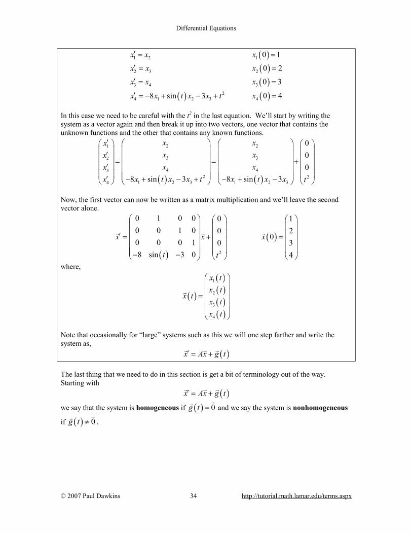
In this case we need to be careful with the t2 in the last equation. We’ll start by writing the system as a vector again and then break it up into two vectors, one vector that contains the unknown functions and the other that contains any known functions.
( ) ( )
2 21
3 32
4 432 2
1 2 3 1 2 34
000
8 sin 3 8 sin 3
x xxx xxx xx
x t x x t x t x xx t
′ ′ = = + ′ ′ − + − + − + −
Now, the first vector can now be written as a matrix multiplication and we’ll leave the second vector alone.
( )
( )2
0 1 0 0 0 10 0 1 0 0 2
00 0 0 1 0 38 sin 3 0 4
x x x
t t
′ = + = − −
r r r
where,
( )
( )( )( )( )
1
2
3
4
x tx t
x tx tx t
=
r
Note that occasionally for “large” systems such as this we will one step farther and write the system as,
( )x Ax g t′ = +r r r
The last thing that we need to do in this section is get a bit of terminology out of the way. Starting with ( )x Ax g t′ = +
r r r
we say that the system is homogeneous if ( ) 0g t =rr
and we say the system is nonhomogeneous
if ( ) 0g t ≠rr
.
Differential Equations
© 2007 Paul Dawkins 35 http://tutorial.math.lamar.edu/terms.aspx
Solutions to Systems Now that we’ve got some of the basic out of the way for systems of differential equations it’s time to start thinking about how to solve a system of differential equations. We will start with the homogeneous system written in matrix form, x A x′ =
r r (1) where, A is an n x n matrix and xr is a vector whose components are the unknown functions in the system. Now, if we start with n = 1 then the system reduces to a fairly simple linear (or separable) first order differential equation. x ax′ = and this has the following solution, ( ) atx t c= e So, let’s use this as a guide and for a general n let’s see if ( ) r tx t η= err (2) will be a solution. Note that the only real difference here is that we let the constant in front of the exponential be a vector. All we need to do then is plug this into the differential equation and see what we get. First notice that the derivative is, ( ) r tx t rη′ = err So upon plugging the guess into the differential equation we get,
( )( )
0
0
r t r t
r t
r t
r A
A r
A rI
η η
η η
η
=
− =
− =
e e
e
e
r rrr rrr
Now, since we know that exponentials are not zero we can drop that portion and we then see that in order for (2) to be a solution to (1) then we must have ( ) 0A rI η− =
rr Or, in order for (2) to be a solution to (1), r and η
r must be an eigenvalue and eigenvector for the
matrix A. Therefore, in order to solve (1) we first find the eigenvalues and eigenvectors of the matrix A and then we can form solutions using (2). There are going to be three cases that we’ll need to look at. The cases are real, distinct eigenvalues, complex eigenvalues and repeated eigenvalues. None of this tells us how to completely solve a system of differential equations. We’ll need the following couple of facts to do this.

Differential Equations
© 2007 Paul Dawkins 36 http://tutorial.math.lamar.edu/terms.aspx
Fact 1. If ( )1x tr
and ( )2x tr are two solutions to a homogeneous system, (1), then
( ) ( )1 1 2 2c x t c x t+r r
is also a solution to the system. 2. Suppose that A is an n x n matrix and suppose that ( )1x tr
, ( )2x tr, …, ( )nx tr
are solutions to a homogeneous system, (1). Define,
( )1 2 nX x x x=r r rL
In other words, X is a matrix whose ith column is the ith solution. Now define, ( )detW X=
We call W the Wronskian. If 0W ≠ then the solutions form a fundamental set of solutions and the general solution to the system is,
( ) ( ) ( ) ( )1 1 2 2 n nx t c x t c x t c x t= + + +r r r rL
Note that if we have a fundamental set of solutions then the solutions are also going to be linearly independent. Likewise, if we have a set of linearly independent solutions then they will also be a fundamental set of solutions since the Wronskian will not be zero.
Differential Equations
© 2007 Paul Dawkins 37 http://tutorial.math.lamar.edu/terms.aspx
Phase Plane Before proceeding with actually solving systems of differential equations there’s one topic that we need to take a look at. This is a topic that’s not always taught in a differential equations class but in case you’re in a course where it is taught we should cover it so that you are prepared for it. Let’s start with a general homogeneous system, x Ax′ =
r r (1) Notice that 0x =
rr is a solution to the system of differential equations. What we’d like to ask is, do the other solutions to the system approach this solution as t increases or do they move away from this solution? We did something similar to this when we classified equilibrium solutions in a previous section. In fact, what we’re doing here is simply an extension of this idea to systems of differential equations. The solution 0x =
rr is called an equilibrium solution for the system. As with the single
differential equations case, equilibrium solutions are those solutions for which 0Ax =
rr We are going to assume that A is a nonsingular matrix and hence will have only one solution, 0x =
rr and so we will have only one equilibrium solution. Back in the single differential equation case recall that we started by choosing values of y and plugging these into the function f(y) to determine values of y′ . We then used these values to sketch tangents to the solution at that particular value of y. From this we could sketch in some solutions and use this information to classify the equilibrium solutions. We are going to do something similar here, but it will be slightly different as well. First we are going to restrict ourselves down to the 2 x 2 case. So, we’ll be looking at systems of the form,
1 1 2
2 1 2
x ax bx a bx x
x cx dx c d′ = + ′⇒ = ′ = +
r r
Solutions to this system will be of the form,
( )( )
1
2
x tx
x t
=
r
and our single equilibrium solution will be,
00
x =
r
In the single differential equation case we were able to sketch the solution, y(t) in the y-t plane and see actual solutions. However, this would somewhat difficult in this case since our solutions are actually vectors. What we’re going to do here is think of the solutions to the system as points

Differential Equations
© 2007 Paul Dawkins 38 http://tutorial.math.lamar.edu/terms.aspx
in the x1-x2 plane and plot these points. Our equilibrium solution will correspond to the origin of x1-x2 plane and the x1-x2 plane is called the phase plane. To sketch a solution in the phase plane we can pick values of t and plug these into the solution. This gives us a point in the x1-x2 or phase plane that we can plot. Doing this for many values of t will then give us a sketch of what the solution will be doing in the phase plane. A sketch of a particular solution in the phase plane is called the trajectory of the solution. Once we have the trajectory of a solution sketched we can then ask whether or not the solution will approach the equilibrium solution as t increases. We would like to be able to sketch trajectories without actually having solutions in hand. There are a couple of ways to do this. We’ll look at one of those here and we’ll look at the other in the next couple of sections. One way to get a sketch of trajectories is to do something similar to what we did the first time we looked at equilibrium solutions. We can choose values of xr (note that these will be points in the phase plane) and compute Axr . This will give a vector that represents x′r at that particular solution. As with the single differential equation case this vector will be tangent to the trajectory at that point. We can sketch a bunch of the tangent vectors and then sketch in the trajectories. This is a fairly work intensive way of doing these and isn’t the way to do them in general. However, it is a way to get trajectories without doing any solution work. All we need is the system of differential equations. Let’s take a quick look at an example. Example 1 Sketch some trajectories for the system,
1 1 2
2 1 2
2 1 23 2 3 2
x x xx x
x x x′ = + ′⇒ = ′ = +
r r
Solution So, what we need to do is pick some points in the phase plane, plug them into the right side of the system. We’ll do this for a couple of points.
1 1 2 1 11 3 2 1 1
2 1 2 2 20 3 2 0 6
3 1 2 3 72 3 2 2 13
x x
x x
x x
− − ′= ⇒ = = − ′= ⇒ = =
− − − ′= ⇒ = = − − −
r r
r r
r r
So, what does this tell us? Well at the point (-1, 1) in the phase plane there will be a vector pointing in the direction 1, 1− . At the point (2,0) there will be a vector pointing in the direction
2,6 . At the point (-3,-2) there will be a vector pointing in the direction 7, 13− − . Doing this for a large number of points in the phase plane will give the following sketch of vectors.

Differential Equations
© 2007 Paul Dawkins 39 http://tutorial.math.lamar.edu/terms.aspx
Now all we need to do is sketch in some trajectories. To do this all we need to do is remember that the vectors in the sketch above are tangent to the trajectories. Also the direction of the vectors give the direction of the trajectory as t increases so we can show the time dependence of the solution by adding in arrows to the trajectories. Doing this gives the following sketch.
This sketch is called the phase portrait. Usually phase portraits only include the trajectories of the solutions and not any vectors. All of our phase portraits form this point on will only include the trajectories. In this case it looks like most of the solutions will start away from the equilibrium solution then as t starts to increase they move in towards the equilibrium solution and then eventually start moving away from the equilibrium solution again. There seem to be four solutions that have slightly different behaviors. It looks like two of the solutions will start at (or near at least) the equilibrium solution and them move straight away from

Differential Equations
© 2007 Paul Dawkins 40 http://tutorial.math.lamar.edu/terms.aspx
it while two other solution start away from the equilibrium solution and then move straight in towards the equilibrium solution. In these kinds of cases we call the equilibrium point a saddle point and we call the equilibrium point in this case unstable since all but two of the solutions are moving away from it as t increases. As we noted earlier this is not generally the way that we will sketch trajectories. All we really need to get the trajectories are the eigenvalues and eigenvectors of the matrix A. We will see how to do this over the next couple of sections as we solve the systems. Here are a few more phase portraits so you can see some more possible examples. We’ll actually be generating several of these throughout the course of the next couple of sections.

Differential Equations
© 2007 Paul Dawkins 41 http://tutorial.math.lamar.edu/terms.aspx
Not all possible phase portraits have been shown here. These are here to show you some of the possibilities. Make sure to notice that several kinds can be either asymptotically stable or unstable depending upon the direction of the arrows. Notice the difference between stable and asymptotically stable. In an asymptotically stable node or spiral all the trajectories will move in towards the equilibrium point as t increases whereas, a center (which is always stable) trajectories will just move around the equilibrium point but never actually move in towards it.

Differential Equations
© 2007 Paul Dawkins 42 http://tutorial.math.lamar.edu/terms.aspx
Real, Distinct Eigenvalues It’s now time to start solving systems of differential equations. We’ve seen that solutions to the system, x Ax′ =
r r will be of the form
tx λη= err
where λ and ηr
are eigenvalues and eigenvectors of the matrix A. We will be working with 2 x 2
systems so this means that we are going to be looking for two solutions, ( )1x trand ( )2x tr
, where the determinant of the matrix, ( )1 2X x x=
r r is nonzero. We are going to start by looking at the case where our two eigenvalues, 1λ and 2λ are real and distinct. In other words they will be real, simple eigenvalues. Recall as well that the eigenvectors for simple eigenvalues are linearly independent. This means that the solutions we get from these will also be linearly independent. If the solutions are linearly independent the matrix X must be nonsingular and hence these two solutions will be a fundamental set of solutions. The general solution in this case will then be, ( ) ( ) ( )1 21 2
1 2t tx t c cλ λη η= +e er rr
Note that each of our examples will actually be broken into two examples. The first example will be solving the system and the second example will be sketching the phase portrait for the system. Phase portraits are not always taught in a differential equations course and so we’ll strip those out of the solution process so that if you haven’t covered them in your class you can ignore the phase portrait example for the system. Example 1 Solve the following IVP.
( )1 2 0, 0
3 2 4x x x ′ = = −
r r r
Solution So, the first thing that we need to do is find the eigenvalues for the matrix.
( )
( )( )
2
1 2
1 2det
3 2
3 41 4 1, 4
A Iλ
λλ
λ λ
λ λ λ λ
−− =
−
= − −
= + − ⇒ = − =
Now let’s find the eigenvectors for each of these.
1 1λ = − : We’ll need to solve,
11 2 1 2
2
2 2 02 2 0
3 3 0η
η η η ηη
= ⇒ + = ⇒ = −

Differential Equations
© 2007 Paul Dawkins 43 http://tutorial.math.lamar.edu/terms.aspx
The eigenvector in this case is,
( )122
2
1, 1
1η
η η ηη− −
= ⇒ = =
r r
2 4λ = : We’ll need to solve,
11 2 1 2
2
3 2 0 23 2 03 2 0 3
ηη η η η
η−
= ⇒ − + = ⇒ = −
The eigenvector in this case is,
( )2
2232
2
2, 3
3η
η η ηη
= ⇒ = =
r r
Then general solution is then,
( ) 41 2
1 21 3
t tx t c c− − = +
e er
Now, we need to find the constants. To do this we simply need to apply the initial conditions.
( ) 1 2
0 1 20
4 1 3x c c
− = = + −
r
All we need to do now is multiply the constants through and we then get two equations (one for each row) that we can solve for the constants. This gives,
1 21 2
1 2
2 0 8 4,3 4 5 5
c cc c
c c− + =
⇒ = − = −+ = −
The solution is then,
( ) 41 28 41 35 5
t tx t − − = − −
e er
Now, let’s take a look at the phase portrait for the system. Example 2 Sketch the phase portrait for the following system.
1 23 2
x x ′ =
r r
Solution From the last example we know that the eigenvalues and eigenvectors for this system are,
( )
( )
11
22
11
1
24
3
λ η
λ η
− = − =
= =
r
r

Differential Equations
© 2007 Paul Dawkins 44 http://tutorial.math.lamar.edu/terms.aspx
It turns out that this is all the information that we will need to sketch the direction field. We will relate things back to our solution however so that we can see that things are going correctly. Well start by sketching lines that follow the direction of the two eigenvectors. This gives,
Now, from the first example our general solution is
( ) 41 2
1 21 3
t tx t c c− − = +
e er
If we have c2 = 0 then the solution is an exponential times a vector and that all the exponential does is affect the magnitude of the vector and the constant c1 will affect both the sign and the magnitude of the vector. In other words, the trajectory in this case will be a straight line that is parallel to the vector, ( )1η
r. Also notice that as t increases the exponential will get smaller and
smaller and hence the trajectory will be moving in towards the origin. If c1>0 the trajectory will be in Quadrant II and if c1<0 the trajectory will be in Quadrant IV. So the line in the graph above marked with ( )1η
r will be a sketch of the trajectory corresponding
to c2 = 0 and this trajectory will approach the origin as t increases. If we now turn things around and look at the solution corresponding to have c1 = 0 we will have a trajectory that is parallel to ( )2η
r. Also, since the exponential will increase as t increases and so in
this case the trajectory will now move away from the origin as t increases. We will denote this with arrows on the lines in the graph above.

Differential Equations
© 2007 Paul Dawkins 45 http://tutorial.math.lamar.edu/terms.aspx
Notice that we could have gotten this information with actually going to the solution. All we really need to do is look at the eigenvalues. Eigenvalues that are negative will correspond to solutions that will move towards the origin as t increase in a direction that is parallel to its eigenvector. Likewise, eigenvalues that are positive move away from the origin as t increases in a direction that will be parallel to its eigenvector. If both constants are in the solution we will have a combination of these behaviors. For large negative t’s the solution will be dominated by the portion that has the negative eigenvalue since in these cases the exponent will be large and positive. Trajectories for large negative t’s will be parallel to ( )1η
r and moving in the same direction.
Solutions for large positive t’s will be dominated by the portion with the positive eigenvalue. Trajectories in this case will be parallel to ( )2η
r and moving in the same direction.
In general, it looks like trajectories will start “near” ( )1η
r, move in towards the origin and then as
they get closer to the origin they will start moving towards ( )2ηr
and then continue up along this vector. Sketching some of these in will give the following phase portrait. Here is a sketch of this with the trajectories corresponding to the eigenvectors marked in blue.

Differential Equations
© 2007 Paul Dawkins 46 http://tutorial.math.lamar.edu/terms.aspx
In this case the equilibrium solution (0,0) is called a saddle point and is unstable. In this case unstable means that solution move away from it as t increases. So, we’ve solved a system in matrix form, but remember that we started out without the systems in matrix form. Now let’s take a quick look at an example of a system that isn’t in matrix form initially. Example 3 Find the solution to the following system.
( )( )
1 1 2 1
2 1 2 2
2 0 0
3 2 0 4
x x x x
x x x x
′ = + =
′ = + = −
Solution We first need to convert this into matrix form. This is easy enough. Here is the matrix form of the system.
( )1 2 0, 0
3 2 4x x x ′ = = −
r r r
This is just the system from the first example and so we’ve already got the solution to this system. Here it is.
( ) 41 28 41 35 5
t tx t − − = − −
e er
Now, since we want to solution to the system not in matrix form let’s go one step farther here. Let’s multiply the constants and exponentials into the vectors and then add up the two vectors.
( )4 48 8 8 8
5 5 5 54 48 812 12
5 5 5 5
t t t t
t t t tx t− −
− −
−= − =
− − −
e e e ee e e e
r
Now, recall,

Differential Equations
© 2007 Paul Dawkins 47 http://tutorial.math.lamar.edu/terms.aspx
( ) ( )( )
1
2
x tx t
x t
=
r
So, the solution to the system is then,
( )
( )
41
42
8 85 5
8 125 5
t t
t t
x t
x t
−
−
= −
= − −
e e
e e
Let’s work another example. Example 4 Solve the following IVP.
( )5 1 1, 0
4 2 2x x x
− ′ = = −
r r r
Solution So, the first thing that we need to do is find the eigenvalues for the matrix.
( )
( ) ( )
2
1 2
5 1det
4 2
7 61 6 1, 6
A Iλ
λλ
λ λ
λ λ λ λ
− −− =
− −
= + +
= + + ⇒ = − = −
Now let’s find the eigenvectors for each of these.
1 1λ = − : We’ll need to solve,
11 2 2 1
2
4 1 04 0 4
4 1 0η
η η η ηη
− = ⇒ − + = ⇒ = −
The eigenvector in this case is,
( )111
1
1, 1
4 4η
η η ηη
= ⇒ = =
r r
2 6λ = − : We’ll need to solve,
11 2 1 2
2
1 1 00
4 4 0η
η η η ηη
= ⇒ + = ⇒ = −
The eigenvector in this case is,
( )222
2
1, 1
1η
η η ηη− −
= ⇒ = =
r r

Differential Equations
© 2007 Paul Dawkins 48 http://tutorial.math.lamar.edu/terms.aspx
Then general solution is then,
( ) 61 2
1 14 1
t tx t c c− − − = +
e er
Now, we need to find the constants. To do this we simply need to apply the initial conditions.
( ) 1 2
1 1 10
2 4 1x c c
− = = +
r
Now solve the system for the constants.
1 21 2
1 2
1 3 2,4 2 5 5c c
c cc c
− = ⇒ = = −+ =
The solution is then,
( ) 61 13 24 15 5
t tx t − − − = −
e er
Now let’s find the phase portrait for this system. Example 5 Sketch the phase portrait for the following system.
5 1
4 2x x
− ′ = −
r r
Solution From the last example we know that the eigenvalues and eigenvectors for this system are,
( )
( )
11
22
11
4
16
1
λ η
λ η
= − =
−
= − =
r
r
This one is a little different from the first one. However it starts in the same way. We’ll first sketch the trajectories corresponding to the eigenvectors. Notice as well that both of the eigenvalues are negative and so trajectories for these will move in towards the origin as t increases. When we sketch the trajectories we’ll add in arrows to denote the direction they take as t increases. Here is the sketch of these trajectories.

Differential Equations
© 2007 Paul Dawkins 49 http://tutorial.math.lamar.edu/terms.aspx
Now, here is where the slight difference from the first phase portrait comes up. All of the trajectories will move in towards the origin as t increases since both of the eigenvalues are negative. The issue that we need to decide upon is just how they do this. This is actually easier than it might appear to be at first. The second eigenvalue is larger than the first. For large and positive t’s this means that the solution for this eigenvalue will be smaller than the solution for the first eigenvalue. Therefore, as t increases the trajectory will move in towards the origin and do so parallel to ( )1η
r. Likewise,
since the second eigenvalue is larger than the first this solution will dominate for large and negative t’s. Therefore, as we decrease t the trajectory will move away from the origin and do so parallel to ( )2η
r.
Adding in some trajectories gives the following sketch.
In these cases we call the equilibrium solution (0,0) a node and it is asymptotically stable. Equilibrium solutions are asymptotically stable if all the trajectories move in towards it as t increases.
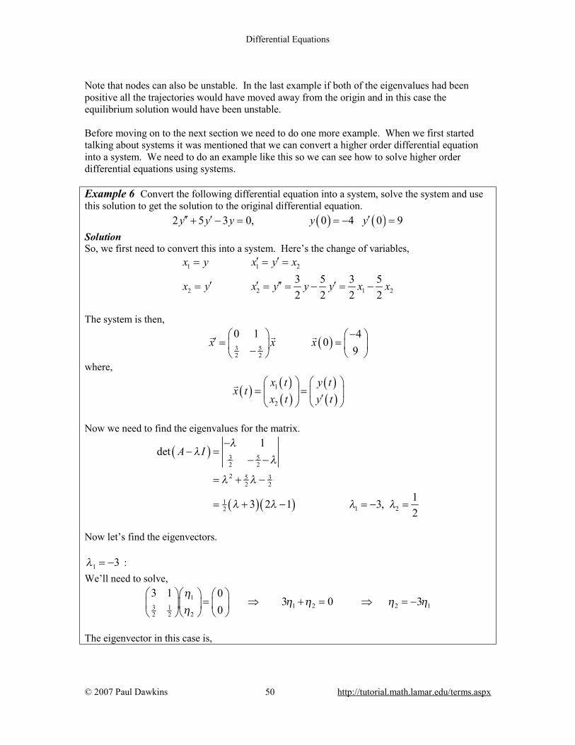
Differential Equations
© 2007 Paul Dawkins 50 http://tutorial.math.lamar.edu/terms.aspx
Note that nodes can also be unstable. In the last example if both of the eigenvalues had been positive all the trajectories would have moved away from the origin and in this case the equilibrium solution would have been unstable. Before moving on to the next section we need to do one more example. When we first started talking about systems it was mentioned that we can convert a higher order differential equation into a system. We need to do an example like this so we can see how to solve higher order differential equations using systems. Example 6 Convert the following differential equation into a system, solve the system and use this solution to get the solution to the original differential equation. ( ) ( )2 5 3 0, 0 4 0 9y y y y y′′ ′ ′+ − = = − = Solution So, we first need to convert this into a system. Here’s the change of variables,
1 1 2
2 2 1 23 5 3 52 2 2 2
x y x y x
x y x y y y x x
′ ′= = =
′ ′ ′′ ′= = = − = −
The system is then,
( )3 52 2
0 1 40
9x x x
− ′ = = −
r r r
where,
( ) ( )( )
( )( )
1
2
x t y tx t
x t y t
= = ′
r
Now we need to find the eigenvalues for the matrix.
( )
( )( )
3 52 2
2 5 32 2
11 22
1det
13 2 1 3,2
A Iλ
λλ
λ λ
λ λ λ λ
−− =
− −
= + −
= + − = − =
Now let’s find the eigenvectors.
1 3λ = − : We’ll need to solve,
11 2 2 13 1
22 2
3 1 03 0 3
0η
η η η ηη
= ⇒ + = ⇒ = −
The eigenvector in this case is,

Differential Equations
© 2007 Paul Dawkins 51 http://tutorial.math.lamar.edu/terms.aspx
( )111
1
1, 1
3 3η
η η ηη
= ⇒ = = − −
r r
1
2 2λ = : We’ll need to solve,
1
121 2 2 13
22
1 0 1 103 0 2 2
ηη η η η
η−
= ⇒ − + = ⇒ = −
The eigenvector in this case is,
( )1 211
12
2, 2
1η
η η ηη
= ⇒ = =
r r
The general solution is then,
( ) 231 2
1 23 1
ttx t c c− = + −
e er
Apply the initial condition.
( ) 1 2
4 1 20
9 3 1x c c
− = = + −
r
This gives the system of equations that we can solve for the constants.
1 21 2
1 2
2 4 22 3,3 9 7 7
c cc c
c c+ = −
⇒ = − = −− + =
The actual solution to the system is then,
( ) 23 1 222 33 17 7
ttx t − = − − −
e er
Now recalling that,
( ) ( )( )
y tx t
y t
= ′
r
we can see that the solution to the original differential equation is just the top row of the solution to the matrix system. The solution to the original differential equation is then,
( ) 2322 67 7
tty t −= − −e e
Notice that as a check, in this case, the bottom row should be the derivative of the top row.

Differential Equations
© 2007 Paul Dawkins 52 http://tutorial.math.lamar.edu/terms.aspx
Complex Eigenvalues In this section we will look at solutions to x Ax′ =
r r where the eigenvalues of the matrix A are complex. With complex eigenvalues we are going to have the same problem that we had back when we were looking at second order differential equations. We want our solutions to only have real numbers in them, however since our solutions to systems are of the form, tx λη= err we are going to have complex numbers come into our solution from both the eigenvalue and the eigenvector. Getting rid of the complex numbers here will be similar to how we did it back in the second order differential equation case, but will involve a little more work this time around. It’s easiest to see how to do this in an example. Example 1 Solve the following IVP.
( )3 9 20
4 3 4x x x
− ′ = = − −
r r r
Solution We first need the eigenvalues and eigenvectors for the matrix.
( )
21,2
3 9det
4 3
27 3 3
A I
i
λλ
λ
λ λ
− −− =
− −
= + = ±
So, now that we have the eigenvalues recall that we only need to get the eigenvector for one of the eigenvalues since we can get the second eigenvector for free from the first eigenvector.
1 3 3 iλ = : We need to solve the following system.
1
2
3 3 3 9 004 3 3 3
i
i
ηη
− − = − −
Using the first equation we get,
( )
( )1 2
2 1
3 3 3 9 0
1 1 33
i
i
η η
η η
− − =
= −
So, the first eigenvector is,
( )
( )
1
1
11
1 1 33
33
1 3
i
i
ηη
η
η η
= −
= =
−
r
r
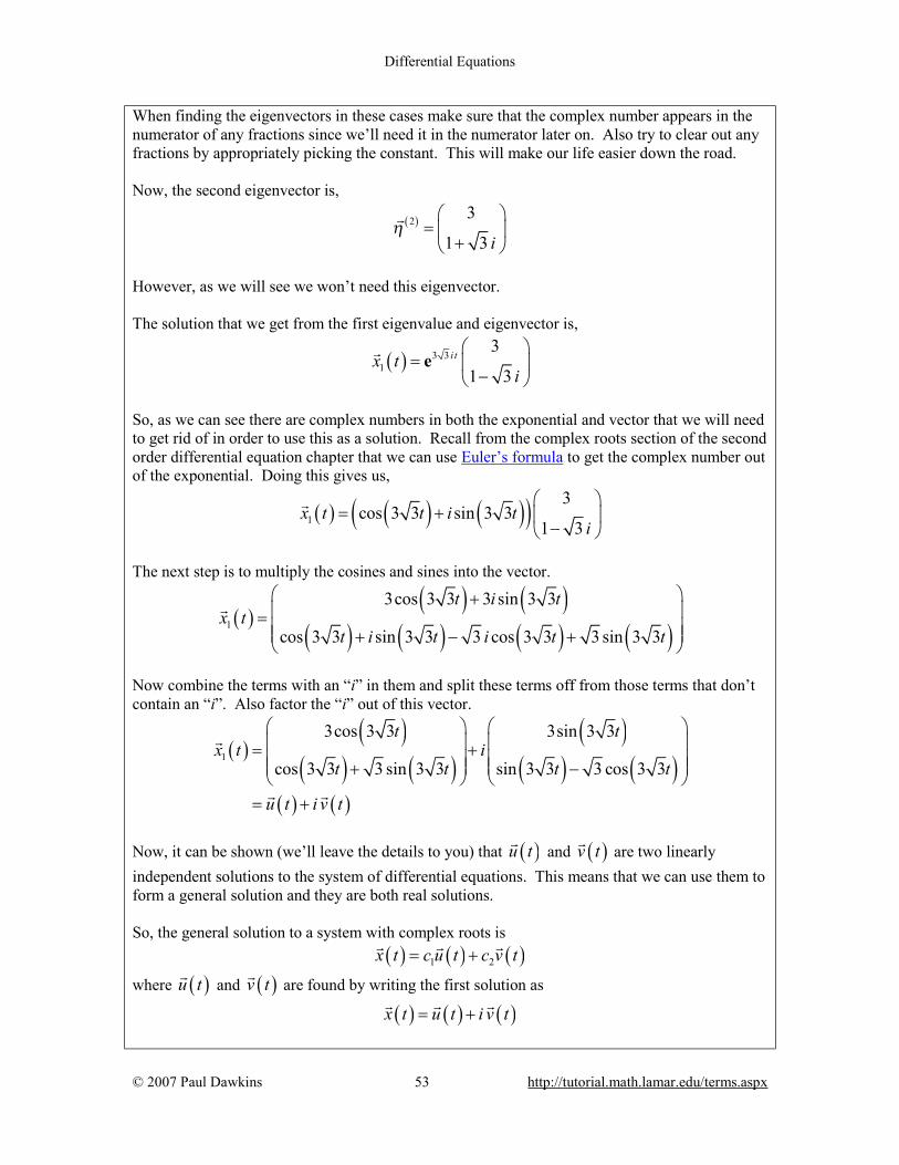
Differential Equations
© 2007 Paul Dawkins 53 http://tutorial.math.lamar.edu/terms.aspx
When finding the eigenvectors in these cases make sure that the complex number appears in the numerator of any fractions since we’ll need it in the numerator later on. Also try to clear out any fractions by appropriately picking the constant. This will make our life easier down the road. Now, the second eigenvector is,
( )2 3
1 3 iη
=
+
r
However, as we will see we won’t need this eigenvector. The solution that we get from the first eigenvalue and eigenvector is,
( ) 3 31
3
1 3i tx t
i
= −
er
So, as we can see there are complex numbers in both the exponential and vector that we will need to get rid of in order to use this as a solution. Recall from the complex roots section of the second order differential equation chapter that we can use Euler’s formula to get the complex number out of the exponential. Doing this gives us,
( ) ( ) ( )( )1
3cos 3 3 sin 3 3
1 3x t t i t
i
= + −
r
The next step is to multiply the cosines and sines into the vector.
( )( ) ( )
( ) ( ) ( ) ( )1
3cos 3 3 3 sin 3 3
cos 3 3 sin 3 3 3 cos 3 3 3 sin 3 3
t i tx t
t i t i t t
+ = + − +
r
Now combine the terms with an “i” in them and split these terms off from those terms that don’t contain an “i”. Also factor the “i” out of this vector.
( )
( )( ) ( )
( )( ) ( )
( ) ( )
1
3cos 3 3 3sin 3 3
cos 3 3 3 sin 3 3 sin 3 3 3 cos 3 3
t tx t i
t t t t
u t i v t
= + + −
= +
r
r r
Now, it can be shown (we’ll leave the details to you) that ( )u tr
and ( )v tr are two linearly
independent solutions to the system of differential equations. This means that we can use them to form a general solution and they are both real solutions. So, the general solution to a system with complex roots is ( ) ( ) ( )1 2x t c u t c v t= +
r r r where ( )u tr
and ( )v tr are found by writing the first solution as
( ) ( ) ( )x t u t i v t= +r r r

Differential Equations
© 2007 Paul Dawkins 54 http://tutorial.math.lamar.edu/terms.aspx
For our system then, the general solution is,
( )( )
( ) ( )( )
( ) ( )1 2
3cos 3 3 3sin 3 3
cos 3 3 3 sin 3 3 sin 3 3 3 cos 3 3
t tx t c c
t t t t
= + + −
r
We now need to apply the initial condition to this to find the constants.
( ) 1 2
02 30
4 1 3x c c
= = + − −
r
This leads to the following system of equations to be solved,
11 2
1 2
3 2 2 14,3 3 33 4
cc c
c c
= ⇒ = =− = −
The actual solution is then,
( )( )
( ) ( )( )
( ) ( )3cos 3 3 3sin 3 32 14
3 3 3cos 3 3 3 sin 3 3 sin 3 3 3 cos 3 3
t tx t
t t t t
= + + −
r
As we did in the last section we’ll do the phase portraits separately from the solution of the system in case phase portraits haven’t been taught in your class. Example 2 Sketch the phase portrait for the system.
3 94 3
x x− ′ = −
r r
Solution When the eigenvalues of a matrix A are purely complex, as they are in this case, the trajectories of the solutions will be circles or ellipses that are centered at the origin. The only thing that we really need to concern ourselves with here are whether they are rotating in a clockwise or counterclockwise direction. This is easy enough to do. Recall when we first looked at these phase portraits a couple of sections ago that if we pick a value of ( )x tr
and plug it into our system we will get a vector that will be tangent to the trajectory at that point and pointing in the direction that the trajectory is traveling.. So, let’s pick the following point and see what we get.
1 3 9 1 30 4 3 0 4
x x− ′= ⇒ = = −
r r
Therefore at the point (1,0) in the phase plane the trajectory will be point in a upwards direction. The only way that this can be is if the trajectories are traveling in a counterclockwise direction. Here is the sketch of some of the trajectories for this problem.

Differential Equations
© 2007 Paul Dawkins 55 http://tutorial.math.lamar.edu/terms.aspx
The equilibrium solution in the case is called a center and is stable. Note in this last example that the equilibrium solution is stable and not asymptotically stable. Asymptotically stable refers to the fact that the trajectories are moving in toward the equilibrium solution as t increases. In this example the trajectories are simply revolving around the equilibrium solution and not moving in towards it. The trajectories are also not moving away from the equilibrium solution and so they aren’t unstable. Therefore we call the equilibrium solution stable. Not all complex eigenvalues will result in centers so let’s take a look at an example where we get something different. Example 3 Solve the following IVP.
( )3 13 30
5 1 10x x x
− ′ = = −
r r r
Solution Let’s get the eigenvalues and eigenvectors for the matrix.
( )
21,2
3 13det
5 1
4 68 2 8
A I
i
λλ
λ
λ λ λ
− −− =
−
= − + = ±
Now get the eigenvector for the first eigenvalue.
1 2 8iλ = + : We need to solve the following system.
1
2
1 8 13 05 1 8 0
ii
ηη
− − = − −
Using the second equation we get,
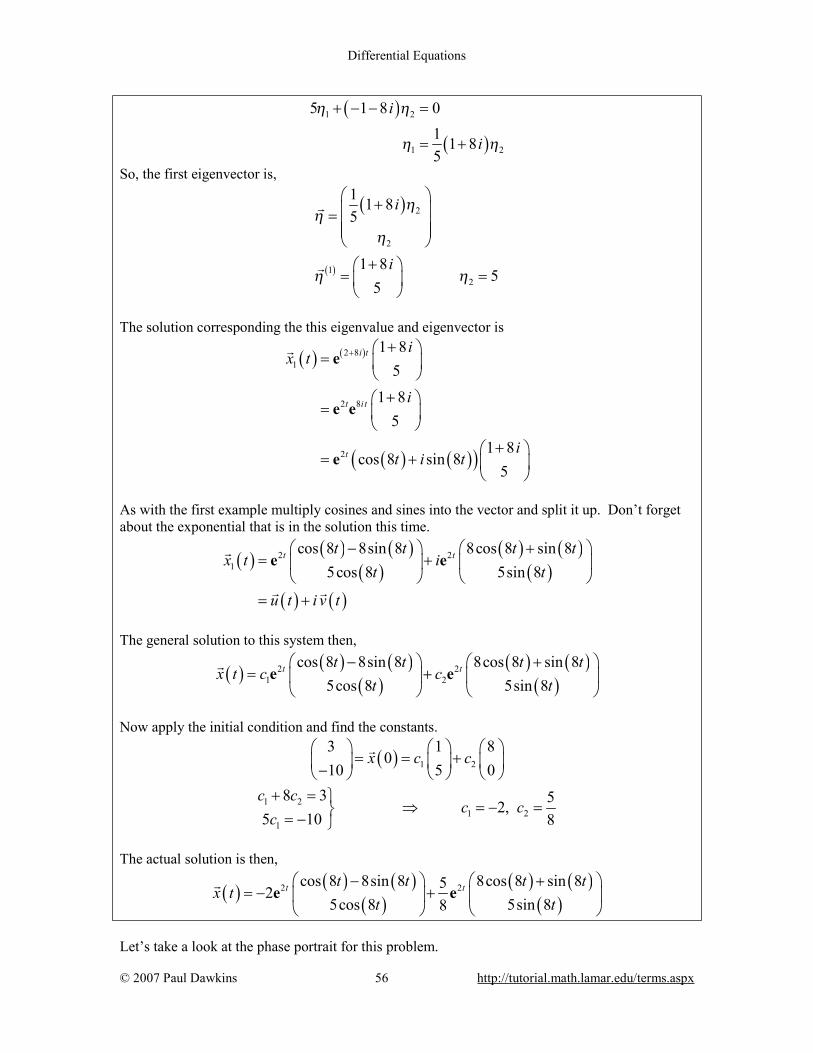
Differential Equations
© 2007 Paul Dawkins 56 http://tutorial.math.lamar.edu/terms.aspx
( )
( )
1 2
1 2
5 1 8 01 1 85
i
i
η η
η η
+ − − =
= +
So, the first eigenvector is,
( )
( )
2
2
12
1 1 85
1 85
5
i
i
ηη
η
η η
+ =
+ = =
r
r
The solution corresponding the this eigenvalue and eigenvector is
( ) ( )
( ) ( )( )
2 81
2 8
2
1 85
1 85
1 8cos 8 sin 8
5
i t
t i t
t
ix t
i
it i t
+ + =
+
=
+ = +
e
e e
e
r
As with the first example multiply cosines and sines into the vector and split it up. Don’t forget about the exponential that is in the solution this time.
( ) ( ) ( )
( )( ) ( )
( )( ) ( )
2 21
cos 8 8sin 8 8cos 8 sin 85cos 8 5sin 8
t tt t t tx t i
t t
u t i v t
− + = +
= +
e er
r r
The general solution to this system then,
( ) ( ) ( )( )
( ) ( )( )
2 21 2
cos 8 8sin 8 8cos 8 sin 85cos 8 5sin 8
t tt t t tx t c c
t t− +
= +
e er
Now apply the initial condition and find the constants.
( ) 1 2
3 1 80
10 5 0x c c
= = + −
r
1 21 2
1
8 3 52,5 10 8
c cc c
c+ =
⇒ = − == −
The actual solution is then,
( ) ( ) ( )( )
( ) ( )( )
2 2cos 8 8sin 8 8cos 8 sin 8525cos 8 5sin 88
t tt t t tx t
t t− +
= − +
e er
Let’s take a look at the phase portrait for this problem.

Differential Equations
© 2007 Paul Dawkins 57 http://tutorial.math.lamar.edu/terms.aspx
Example 4 Sketch the phase portrait for the system.
3 135 1
x x− ′ =
r r
Solution When the eigenvalues of a system are complex with a real part the trajectories will spiral into or out of the origin. We can determine which one it will be by looking at the real portion. Since the real portion will end up being the exponent of an exponential function (as we saw in the solution to this system) if the real part is positive the solution will grow very large as t increases. Likewise, if the real part is negative the solution will die out as t increases. So, if the real part is positive the trajectories will spiral out from the origin and if the real part is negative they will spiral into the origin. We determine the direction of rotation (clockwise vs. counterclockwise) in the same way that we did for the center. In our case the trajectories will spiral out from the origin since the real part is positive and
3 13 1 35 1 0 5
x− ′ = =
r
will rotate in the counterclockwise direction as the last example did. Here is a sketch of some of the trajectories for this system.
Here we call the equilibrium solution a spiral (oddly enough…) and in this case it’s unstable since the trajectories move away from the origin. If the real part of the eigenvalue is negative the trajectories will spiral into the origin and in this case the equilibrium solution will be asymptotically stable.

Differential Equations
© 2007 Paul Dawkins 58 http://tutorial.math.lamar.edu/terms.aspx
Repeated Eigenvalues This is the final case that we need to take a look at. In this section we are going to look at solutions to the system, x Ax′ =
r r where the eigenvalues are repeated eigenvalues. Since we are going to be working with systems in which A is a 2 x 2 matrix we will make that assumption from the start. So the system will have a double eigenvalue, λ. This presents us with a problem. We want two linearly independent solutions so that we can form a general solution. However, with a double eigenvalue we will have only one, 1
tx λη= err So, we need to come up with a second solution. Recall that when we looked at the double root case with the second order differential equations we ran into a similar problem. In that section we simply added a t to the solution and were able to get a second solution. Let’s see if the same thing will work in this case as well. We’ll see if tx t λ η= e rr will also be a solution. To check all we need to do is plug into the system. Don’t forget to product rule the proposed solution when you differentiate! t t tt A tλ λ λη λη η+ =e e er r r Now, we got two functions here on the left side, an exponential by itself and an exponential times a t. So, in order for our guess to be a solution we will need to require,
( ) 0
0
A A Iη λη λ η
η
= ⇒ − =
=
rr r rrr
The first requirement isn’t a problem since we this just says that λ is an eigenvalue and it’s eigenvector is η
r. We already knew this however so there’s nothing new there. The second
however is a problem. Since ηr
is an eigenvector we know that it can’t be zero, yet in order to satisfy the second condition it would have to be. So, our guess was incorrect. The problem seems to be that there is a lone term with just an exponential in it so let’s see if we can’t fix up our guess to correct that. Let’s try the following guess. t tx t λ λη ρ= +e er rr where ρ
r is an unknown vector that we’ll need to determine.
As with the first guess let’s plug this into the system and see what we get.
( )
( )
t t t t t
t t t t
t A t
t A t A
λ λ λ λ λ
λ λ λ λ
η λη λρ η ρ
η λρ λη η ρ
+ + = +
+ + = +
e e e e e
e e e e
r r r r r
r r r r r
Now set coefficients equal again,

Differential Equations
© 2007 Paul Dawkins 59 http://tutorial.math.lamar.edu/terms.aspx
( )( )
0A A I
A A I
λη η λ η
η λρ ρ λ ρ η
= ⇒ − =
+ = ⇒ − =
rr r r
r r r r r
As with our first guess the first equation tells us nothing that we didn’t already know. This time the second equation is not a problem. All the second equation tells us is that ρ
r must be a
solution to this equation. It looks like our second guess worked. Therefore, 2
t tx t λ λη ρ= +e er rr will be a solution to the system provided ρ
r is a solution to
( )A Iλ ρ η− =r r
Also this solution and the first solution are linearly independent and so they form a fundamental set of solutions and so the general solution in the double eigenvalue case is, ( )1 2
t t tx c c tλ λ λη η ρ= + +e e er r rr Let’s work an example. Example 1 Solve the following IVP.
( )7 1 20
4 3 5x x x ′ = = − −
r r r
Solution First find the eigenvalues for the system.
( )
( )
2
21,2
7 1det
4 3
10 25
5 5
A Iλ
λλ
λ λ
λ λ
−− =
− −
= − +
= − ⇒ =
So, we got a double eigenvalue. Of course that shouldn’t be too surprising given the section that we’re in. Let’s find the eigenvector for this eigenvalue.
11 2 2 1
2
2 1 02 0 2
4 2 0η
η η η ηη
= ⇒ + = = − − −
The eigenvector is then,
( )
11
1
11
02
11
2
ηη η
η
η η
= ≠ −
= = −
r
r
The next step is find ρ
r. To do this we’ll need to solve,

Differential Equations
© 2007 Paul Dawkins 60 http://tutorial.math.lamar.edu/terms.aspx
11 2 2 1
2
2 1 12 1 1 2
4 2 2ρ
ρ ρ ρ ρρ
= ⇒ + = = − − − −
Note that this is almost identical to the system that we solve to find the eigenvalue. The only difference is the right hand side. The most general possible ρ
r is
11
1
0if 0
1 2 1ρ
ρ ρ ρρ
= ⇒ = = −
r r
In this case, unlike the eigenvector system we can choose the constant to be anything we want, so we might as well pick it to make our life easier. This usually means picking it to be zero. We can now write down the general solution to the system.
( ) 5 5 51 2
1 1 02 2 1
t t tx t c c t
= + + − − e e er
Applying the initial condition to find the constants gives us,
( ) 1 2
2 1 00
5 2 1x c c
= = + − −
r
11 2
1 2
22, 1
2 5c
c cc c
= ⇒ = = −− + = −
The actual solution is then,
( ) 5 5 5
5 5 5
5 5
1 1 02
2 2 1
2 1 04 2 1
2 15 2
t t t
t t t
t t
x t t
t
t
= − + − −
= − − − −
= − − −
e e e
e e e
e e
r
Note that we did a little combining here to simplify the solution up a little. So, the next example will be to sketch the phase portrait for this system. Example 2 Sketch the phase portrait for the system.
7 14 3
x x ′ = −
r r
Solution These will start in the same way that real, distinct eigenvalue phase portraits start. We’ll first sketch in a trajectory that is parallel to the eigenvector and note that since the eigenvalue is positive the trajectory will be moving away from the origin.

Differential Equations
© 2007 Paul Dawkins 61 http://tutorial.math.lamar.edu/terms.aspx
Now, it will be easier to explain the remainder of the phase portrait if we actually have one in front of us. So here is the full phase portrait with some more trajectories sketched in.
Trajectories in these cases always emerge from (or move into) the origin in a direction that is parallel to the eigenvector. Likewise they will start in one direction before turning around and moving off into the other direction. The directions in which they move are opposite depending on which side of the trajectory corresponding to the eigenvector we are on. Also, as the trajectories moves away from the origin it should start becoming parallel to the trajectory corresponding to the eigenvector. So, how do we determine the direction? We can do the same thing that we did in the complex case. We’ll plug in (1,0) into the system and see which direction the trajectories are moving at that point. Since this point is directly to the right of the origin the trajectory at that point must have already turned around and so this will give the direction that it will traveling after turning around. Doing that for this problem to check our phase portrait gives,

Differential Equations
© 2007 Paul Dawkins 62 http://tutorial.math.lamar.edu/terms.aspx
7 1 1 74 3 0 4
= − −
This vector will point down into the fourth quadrant and so the trajectory must be moving into the fourth quadrant as well. This does match up with our phase portrait. In these cases the equilibrium is called a node and is unstable in this case. Note that sometimes you will hear nodes for the repeated eigenvalue case called degenerate nodes or improper nodes. Let’s work one more example. Example 3 Solve the following IVP.
( )32
16
1 12
2 0x x x
− ′ = = − −
r r r
Solution First the eigenvalue for the system.
( )32
16
2
2
1,2
1det
2934
3 32 2
A Iλ
λλ
λ λ
λ λ
− −− =
− − −
= + +
= + ⇒ = −
Now let’s get the eigenvector.
31
12 21 2 1 21 1
26 2
0 1 3 0 30 2 2
ηη η η η
η
= ⇒ + = = − − −
( )
22
2
12
30
31
1
ηη η
η
η η
− = ≠
−
= =
r
r
Now find ρ
r,
31
12 21 2 1 21 1
26 2
3 1 3 3 6 31 2 2
ρρ ρ ρ ρ
ρ−
= ⇒ + = − = − − − −
22
2
6 3 6if 0
0ρ
ρ ρ ρρ
− − − = ⇒ = =
r r
The general solution for the system is then,
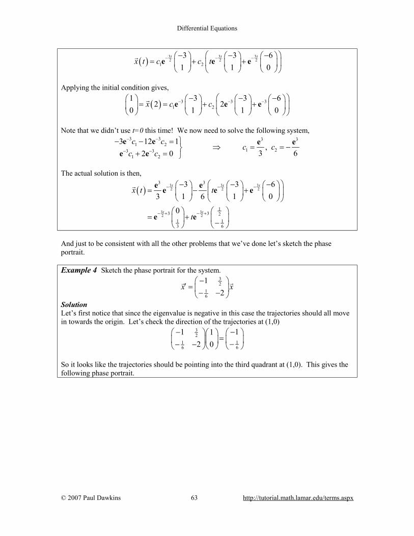
Differential Equations
© 2007 Paul Dawkins 63 http://tutorial.math.lamar.edu/terms.aspx
( )3 3 32 2 2
1 2
3 3 61 1 0
t t tx t c c t− − −− − −
= + +
e e er
Applying the initial condition gives,
( ) 3 3 31 2
1 3 3 62 2
0 1 1 0x c c− − −− − −
= = + +
e e er
Note that we didn’t use t=0 this time! We now need to solve the following system,
3 3 3 3
1 21 23 3
1 2
3 12 1,
3 62 0c c
c cc c
− −
− −
− − =⇒ = = −
+ =
e e e ee e
The actual solution is then,
( )
3 3 32 2 2
3 32 2
3 3
13 3 2
1 13 6
3 3 61 1 03 6
0
t t t
t t
x t t
t
− − −
− + − +
− − − = − +
= + −
e ee e e
e e
r
And just to be consistent with all the other problems that we’ve done let’s sketch the phase portrait. Example 4 Sketch the phase portrait for the system.
32
16
12
x x−
′ = − −
r r
Solution Let’s first notice that since the eigenvalue is negative in this case the trajectories should all move in towards the origin. Let’s check the direction of the trajectories at (1,0)
32
1166
11 12 0
−− = −− −
So it looks like the trajectories should be pointing into the third quadrant at (1,0). This gives the following phase portrait.
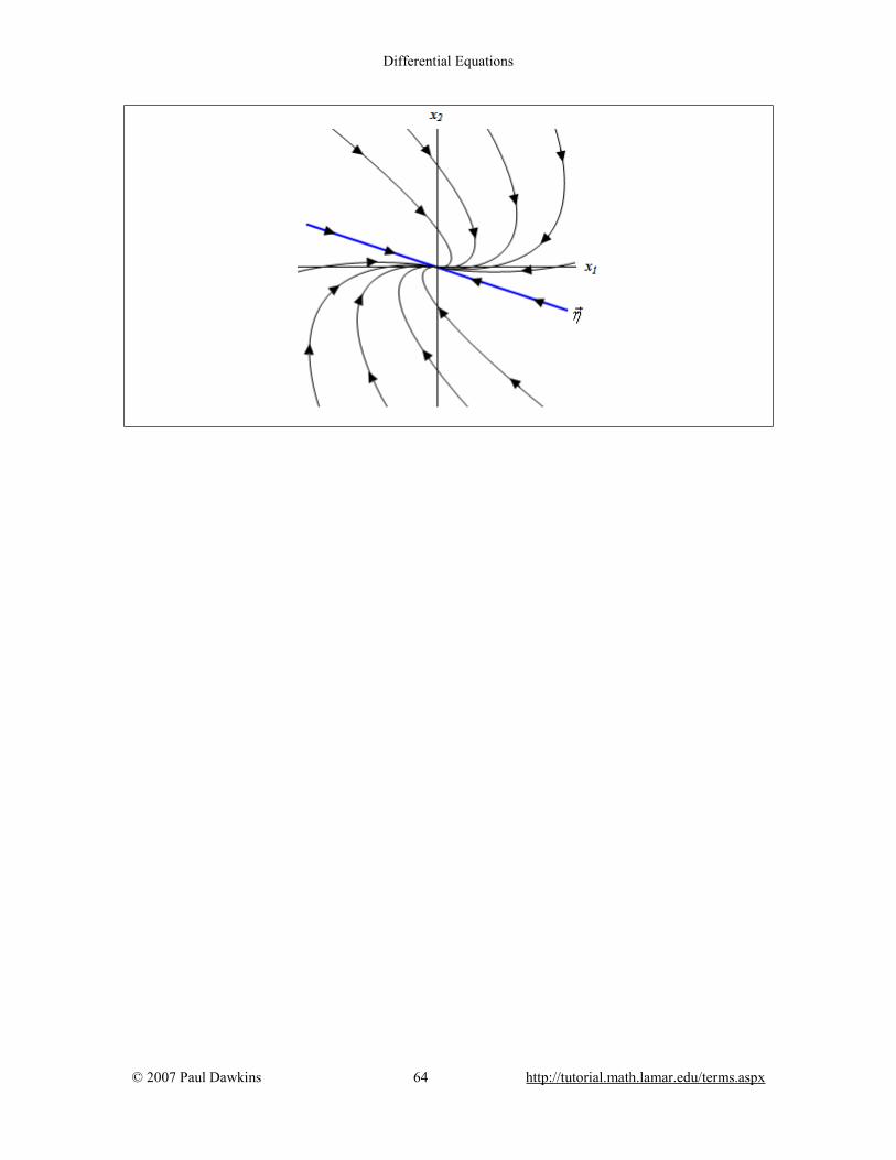
Differential Equations
© 2007 Paul Dawkins 64 http://tutorial.math.lamar.edu/terms.aspx

Differential Equations
© 2007 Paul Dawkins 65 http://tutorial.math.lamar.edu/terms.aspx
Nonhomogeneous Systems We now need to address nonhomogeneous systems briefly. Both of the methods that we looked at back in the second order differential equations chapter can also be used here. As we will see Undetermined Coefficients is almost identical when used on systems while Variation of Parameters will need to have a new formula derived, but will actually be slightly easier when applied to systems. Undetermined Coefficients The method of Undetermined Coefficients for systems is pretty much identical to the second order differential equation case. The only difference is that the coefficients will need to be vectors now. Let’s take a quick look at an example. Example 1 Find the general solution to the following system.
1 2 23 2 4
x x t ′ = + −
r r
Solution We already have the complimentary solution as we solved that part back in the real eigenvalue section. It is,
( ) 41 2
1 21 3
t tcx t c c− −
= +
e er
Guessing the form of the particular solution will work in exactly the same way it did back when we first looked at this method. We have a linear polynomial and so our guess will need to be a linear polynomial. The only difference is that the “coefficients” will need to be vectors instead of constants. The particular solution will have the form,
1 1
2 2P
a bx ta b t
a b
= + = +
rr r
So, we need to differentiate the guess
1
2P
ax a
a ′ = =
r r
Before plugging into the system let’s simplify the notation a little to help with our work. We’ll write the system as,
1 2 23 2 4
x x t Ax tg ′ = + = + −
r r r r
This will make the following work a little easier. Now, let’s plug things into the system.
Differential Equations
© 2007 Paul Dawkins 66 http://tutorial.math.lamar.edu/terms.aspx
( )
( ) ( )0
a A ta b tg
a tAa Ab tg
t Aa g Ab a
= + +
= + +
= + + −
rr r r
rr r rrr r r r
Now we need to set the coefficients equal. Doing this gives,
1
0
: 0
: 0
t Aa g Aa g
t Ab a Ab a
+ = = −
− = =
rr r r rr rrr r
Now only ar is unknown in the first equation so we can use Gaussian elimination to solve the system. We’ll leave this work to you to check.
15
2 2
31 2 23 2 4
aa
a
= − ⇒ = −−
r
Now that we know ar we can solve the second equation for b
r.
11
1 45 23
2 2 8
31 23 2
bb
b−
= ⇒ = −
r
So, since we were able to solve both equations, the particular solution is then,
114
5 232 8
3Px t
− = + −
r
The general solution is then,
( )1144
1 2 5 232 8
31 21 3
t tx t c c t− −− = + + + −
e er
So, as you can see undetermined coefficients is nearly the same as the first time we saw it. The work in solving for the “constants” is a little messier however. Variation of Parameters In this case we will need to derive a new formula for variation of parameters for systems. The derivation this time will be much simpler than the when we first saw variation of parameters. First let X(t) be a matrix whose ith column is the ith linearly independent solution to the system, x Ax′ =
r r Now it can be shown that X(t) will be a solution to the following differential equation. X AX′ = (1) This is nothing more than the original system with the matrix in place of the original vector. We are going to try and find a particular solution to ( )x Ax g t′ = +
r r r

Differential Equations
© 2007 Paul Dawkins 67 http://tutorial.math.lamar.edu/terms.aspx
We will assume that we can find a solution of the form, ( ) ( )Px X t v t=
r r
where we will need to determine the vector ( )v tr. To do this we will need to plug this into the
nonhomogeneous system. Don’t forget to product rule the particular solution when plugging the guess into the system. X v X v A X v g′ ′+ = +
r r r r Note that we dropped the “(t)” part of things to simplify the notation a little. Now using (1) we can rewrite this a little.
X v X v X v g
X v g′ ′ ′+ = +
′ =
r r r rr r
Because we formed X using linearly independent solutions we know that det(X) must be nonzero and this in turn means that we can find the inverse of X. So, multiply both sides by the inverse of X. 1v X g−′ =
r r Now all that we need to do is integrate both sides to get ( )v tr
.
( ) 1v t X g dt−= ∫r r
As with the second order differential equation case we can ignore any constants of integration. The particular solution is then, 1
Px X X g dt−= ∫r r (2)
Let’s work a quick example using this. Example 2 Find the general solution to the following system.
25 1 64 2 1
tx x− ′ = + − −
er r
Solution We found the complimentary solution to this system in the real eigenvalue section. It is,
( ) 61 2
1 14 1
t tcx t c c− − −
= +
e er
Now the matrix X is,
6
64
t t
t tX− −
− −
−=
e ee e
Now, we need to find the inverse of this matrix. We saw how to find inverses of matrices back in the second linear algebra review section and the process is the same here even though we don’t have constant entries. We’ll leave the detail to you to check.

Differential Equations
© 2007 Paul Dawkins 68 http://tutorial.math.lamar.edu/terms.aspx
1 1
1 5 56 64 1
5 5
t t
t tX − =
−
e ee e
Now do the multiplication in the integral.
2 31 1
1 5 56 6 2 84 1
5 5
65
t t t t
t t t tX g− = = − − −
e e e ee e e e
r
Now do the integral.
3 33 1
1 388 58
85 5
t tt
tt t
dtX g dt dt
dt−
= = = −− −
⌠⌡
∫∫
∫
e eeee e
r
Remember that to integrate a matrix or vector you just integrate the individual entries. We can now get the particular solution.
1
36 13
86 58
22324
21724
232421724
4
P
tt t
tt t
t
t
t
x X X g dt−
− −
− −
=
−= −
=
=
∫ee eee e
ee
e
r r
The general solution is then,
( )23246 2
1 2 1724
1 14 1
t t tx t c c− − − = + +
e e er
So, some of the work can be a little messy, but overall not too bad. We looked at two methods of solving nonhomogeneous differential equations here and while the work can be a little messy they aren’t too bad. Of course we also kept the nonhomogeneous part fairly simple here. More complicated problems will have significant amounts of work involved.

Differential Equations
© 2007 Paul Dawkins 69 http://tutorial.math.lamar.edu/terms.aspx
Laplace Transforms There’s not too much to this section. We’re just going to work an example to illustrate how Laplace transforms can be used to solve systems of differential equations. Example 1 Solve the following system.
( )( )
1 1 2 1
2 1 2
3 3 2 0 1
6 0 1
x x x x
x x t x
′ = − + =
′ = − − = −
Solution First notice that the system is not given in matrix form. This is because the system won’t be solved in matrix form. Also note that the system is nonhomogeneous. We start just as we did when we used Laplace transforms to solve single differential equations. We take the transform of both differential equations.
( ) ( ) ( ) ( )
( ) ( ) ( )
1 1 1 2
2 2 1 2
20 3 3
10 6
sX s x X s X ss
sX s x X ss
− = − +
− = − −
Now plug in the initial condition and simplify things a little.
( ) ( ) ( )
( ) ( )
1 2
2
1 2 2 2
2 23 3 1
1 16 1
ss X s X ss s
sX s sX ss s
+− + = + =
++ = − − = −
Now we need to solve this for one of the transforms. We’ll do this by multiplying the top equation by s and the bottom by -3 and then adding. This gives,
( ) ( )2
21 2
3 33 18 2 ss s X s ss
+− − = + +
Solving for X1 gives,
( ) ( ) ( )3 2
1 2
5 33 6
s sX ss s s
+ +=
+ −
Partial fractioning gives,
( )1 2
1 133 28 3 18108 6 3
X ss s s s
= − + − − +
Taking the inverse transform gives us the first solution,
( ) ( )6 31
1 133 28 3 18108
t tx t t−= − + −e e
Now to find the second solution we could go back up and eliminate X1 to find the transform for X2 and sometimes we would need to do that. However, in this case notice that the second

Differential Equations
© 2007 Paul Dawkins 70 http://tutorial.math.lamar.edu/terms.aspx
differential equation is, 2 1 2 16 6x x t x x t dt′ = − − ⇒ = − −∫ So, plugging the first solution in and integrating gives,
( )
( )
6 32
6 3
1 133 28 318
1 133 56 18108
t t
t t
x t dt
t c
−
−
= − − +
= − + + +
∫ e e
e e
Now, reapplying the second initial condition to get the constant of integration gives
( )1 31 133 56108 4
c c− = − + + ⇒ =
The second solution is then,
( ) ( )6 32
1 133 56 18 81108
t tx t t−= − + + −e e
So, putting all this together gives the solution to the system as,
( ) ( )
( ) ( )
6 31
6 32
1 133 28 3 18108
1 133 56 18 81108
t t
t t
x t t
x t t
−
−
= − + −
= − + + −
e e
e e
Compared to the last section the work here wasn’t too bad. That won’t always be the case of course, but you can see that using Laplace transforms to solve systems isn’t too bad in at least some cases.

Differential Equations
© 2007 Paul Dawkins 71 http://tutorial.math.lamar.edu/terms.aspx
Modeling In this section we’re going to go back and revisit the idea of modeling only this time we’re going to look at it in light of the fact that we now know how to solve systems of differential equations. We’re not actually going to be solving any differential equations in this section. Instead we’ll just be setting up a couple of problems that are extensions of some of the work that we’ve done in earlier modeling sections whether it is the first order modeling or the vibrations work we did in the second order chapter. Almost all of the systems that we’ll be setting up here will be nonhomogeneous systems (which we only briefly looked at), will be nonlinear (which we didn’t look at) and/or will involve systems with more than two differential equations (which we didn’t look at, although most of what we do know will still be true). Mixing Problems Let’s start things by looking at a mixing problem. The last time we saw these was back in the first order chapter. In those problems we had a tank of liquid with some type of contaminate dissolved in it. Liquid, possibly with more contaminate dissolved in it, entered the tank and liquid left the tank. In this situation we want to extend things out to the following situation.
We’ll now have two tanks that are interconnected with liquid potentially entering both and with an exit for some of the liquid if we need it (as illustrated by the lower connection). For this situation we’re going to make the following assumptions.
1. The inflow and outflow from each tank are equal, or in other words the volume in each tank is constant. When we worked with a single tank we didn’t need to worry about this, but here if we don’t well end up with a system with nonconstant coefficients and those can be quite difficult to solve.
2. The concentration of the contaminate in each tank is the same at each point in the tank. In reality we know that this won’t be true but without this assumption we’d need to deal with partial differential equations.
3. The concentration of contaminate in the outflow from tank 1 (the lower connection in the figure above) is the same as the concentration in tank 1. Likewise, the concentration of contaminate in the outflow from tank 2 (the upper connection) is the same as the concentration in tank 2.

Differential Equations
© 2007 Paul Dawkins 72 http://tutorial.math.lamar.edu/terms.aspx
4. The outflow from tank 1 is split and only some of the liquid exiting tank 1 actually reaches tank 2. The remainder exits the system completely. Note that if we don’t want any liquid to completely exit the system we can think of the exit as having a value that is turned off. Also note that we could just as easily done the same thing for the outflow from tank 2 if we’d wanted to.
Let’s take a look at a quick example. Example 2 Two 1000 liter tanks are with salt water. Tank 1 contains 800 liters of water initially containing 20 grams of salt dissolved in it and tank 2 contains 1000 liters of water and initially has 80 grams of salt dissolved in it. Salt water with a concentration of ½ gram/liter of salt enters tank 1 at a rate of 4 liters/hour. Fresh water enters tank 2 at a rate of 7 liters/hour. Through a connecting pipe water flows from tank 2 into tank 1 at a rate of 10 liters/hour. Through a different connecting pipe 14 liters/hour flows out of tank 1 and 11 liters/hour are drained out of the pipe (and hence out of the system completely) and only 3 liters/hour flows back into tank 2. Set up the system that will give the amount of salt in each tank at any given time. Solution Okay, let ( )1Q t and ( )2Q t be the amount of salt in tank 1 and tank 2 at any time t respectively. Now all we need to do is set up a differential equation for each tank just as we did back when we had a single tank. The only difference is that we now need to deal with the fact that we’ve got a second inflow to each tank and the concentration of the second inflow will be the concentration of the other tank. Recall that the basic differential equation is the rate of change of salt ( Q′ ) equals the rate at which salt enters minus the rate at salt leaves. Each entering/leaving rate is found by multiplying the flow rate times the concentration. Here is the differential equation for tank 1.
( ) ( ) ( ) ( )2 1
1 1
2 1
14 10 14 0 202 1000 800
72100 400
Q QQ Q
Q Q
′ = + − =
= + −
In this differential equation the first pair of numbers is the salt entering from the external inflow. The second set of numbers is the salt that entering into the tank from the water flowing in from tank 2. The third set is the salt leaving tank as water flows out. Here’s the second differential equation.
( ) ( ) ( ) ( ) ( )1 2
2 2
1 2
7 0 3 10 0 80800 1000
3800 100
Q QQ Q
Q Q
′ = + − =
= −
Note that because the external inflow into tank 2 is fresh water the concentration of salt in this is zero.

Differential Equations
© 2007 Paul Dawkins 73 http://tutorial.math.lamar.edu/terms.aspx
In summary here is the system we’d need to solve,
( )
( )
2 11 1
1 22 2
72 0 20100 400
3 0 80800 100
Q QQ Q
Q QQ Q
′ = + − =
′ = − =
This is a nonhomogeneous system because of the first term in the first differential equation. If we had fresh water flowing into both of these we would in fact have a homogeneous system. Population The next type of problem to look at is the population problem. Back in the first order modeling section we looked at some population problems. In those problems we looked at a single population and often included some form of predation. The problem in that section was we assumed that the amount of predation would be constant. This however clearly won’t be the case in most situations. The amount of predation will depend upon the population of the predators and the population of the predators will depend, as least partially, upon the population of the prey. So, in order to more accurately (well at least more accurate than what we originally did) we really need to set up a model that will cover both populations, both the predator and the prey. These types of problems are usually called predator-prey problems. Here are the assumptions that we’ll make when we build up this model.
1. The prey will grow at a rate that is proportional to its current population if there are no predators.
2. The population of predators will decrease at a rate proportional to its current population if there is no prey.
3. The number of encounters between predator and prey will be proportional to the product of the populations.
4. Each encounter between the predator and prey will increase the population of the predator and decrease the population of the prey.
So, given these assumptions let’s write down the system for this case. Example 3 Write down the system of differential equations for the population of predators and prey using the assumptions above. Solution We’ll start off by letting x represent the population of the predators and y represent the population of the prey. Now, the first assumption tells us that, in the absence of predators, the prey will grow at a rate of ay where 0a > . Likewise the second assumption tells us that, in the absence of prey, the predators will decrease at a rate of bx− where 0b > . Next, the third and fourth assumptions tell us how the population is affected by encounters between predators and prey. So, with each encounter the population of the predators will increase
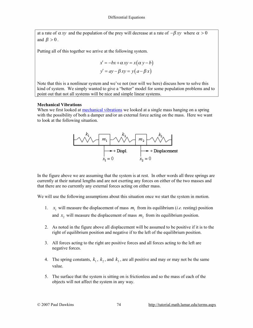
Differential Equations
© 2007 Paul Dawkins 74 http://tutorial.math.lamar.edu/terms.aspx
at a rate of xyα and the population of the prey will decrease at a rate of xyβ− where 0α > and 0β > . Putting all of this together we arrive at the following system.
( )
( )x bx xy x y b
y ay xy y a x
α α
β β
′ = − + = −
′ = − = −
Note that this is a nonlinear system and we’ve not (nor will we here) discuss how to solve this kind of system. We simply wanted to give a “better” model for some population problems and to point out that not all systems will be nice and simple linear systems. Mechanical Vibrations When we first looked at mechanical vibrations we looked at a single mass hanging on a spring with the possibility of both a damper and/or an external force acting on the mass. Here we want to look at the following situation.
In the figure above we are assuming that the system is at rest. In other words all three springs are currently at their natural lengths and are not exerting any forces on either of the two masses and that there are no currently any external forces acting on either mass. We will use the following assumptions about this situation once we start the system in motion.
1. 1x will measure the displacement of mass 1m from its equilibrium (i.e. resting) position and 2x will measure the displacement of mass 2m from its equilibrium position.
2. As noted in the figure above all displacement will be assumed to be positive if it is to the right of equilibrium position and negative if to the left of the equilibrium position.
3. All forces acting to the right are positive forces and all forces acting to the left are negative forces.
4. The spring constants, 1k , 2k , and 3k , are all positive and may or may not be the same value.
5. The surface that the system is sitting on is frictionless and so the mass of each of the objects will not affect the system in any way.

Differential Equations
© 2007 Paul Dawkins 75 http://tutorial.math.lamar.edu/terms.aspx
Before writing down the system for this case recall that the force exerted by the spring on the each mass is the spring constant times the amount that the spring has been compressed or stretched and we’ll need to be careful with signs to make sure that the force is acting in the correct direction. Example 4 Write down the system of differential equations for the spring and mass system above. Solution To help us out let’s first take a quick look at a situation in which both of the masses have been moved. This is shown below.
Before proceeding let’s note that this is only a representation of a typical case, but most definitely not all possible cases. In this case we’re assuming that both 1x and 2x are positive and that 2 1 0x x− < , or in other words, both masses have been moved to the right of their respective equilibrium points and that
1m has been moved farther than 2m . So, under these assumption on 1x and 2x we know that the spring on the left (with spring constant 1k ) has been stretched past it’s natural length while the middle spring (spring constant 2k ) and the right spring (spring constant 3k ) are both under compression. Also, we’ve shown the external forces, ( )1F t and ( )2F t , as present and acting in the positive direction. They do not, in practice, need to be present in every situation in which case we will assume that ( )1 0F t = and/or ( )2 0F t = . Likewise, if the forces are in fact acting in the
negative direction we will then assume that ( )1 0F t < and/or ( )2 0F t < . Before proceeding we need to talk a little bit about how the middle spring will behave as the masses move. Here are all the possibilities that we can have and the affect each will have on
2 1x x− . Note that in each case the amount of compression/stretch in the spring is given by
2 1x x− although we won’t be using the absolute value bars when we set up the differential equations.
1. If both mass move the same amount in the same direction then the middle spring will not have changed length and we’ll have 2 1 0x x− = .
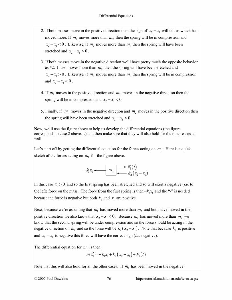
Differential Equations
© 2007 Paul Dawkins 76 http://tutorial.math.lamar.edu/terms.aspx
2. If both masses move in the positive direction then the sign of 2 1x x− will tell us which has moved more. If 1m moves more than 2m then the spring will be in compression and
2 1 0x x− < . Likewise, if 2m moves more than 1m then the spring will have been stretched and 2 1 0x x− > .
3. If both masses move in the negative direction we’ll have pretty much the opposite behavior as #2. If 1m moves more than 2m then the spring will have been stretched and
2 1 0x x− > . Likewise, if 2m moves more than 1m then the spring will be in compression and 2 1 0x x− < .
4. If 1m moves in the positive direction and 2m moves in the negative direction then the spring will be in compression and 2 1 0x x− < .
5. Finally, if 1m moves in the negative direction and 2m moves in the positive direction then the spring will have been stretched and 2 1 0x x− > .
Now, we’ll use the figure above to help us develop the differential equations (the figure corresponds to case 2 above…) and then make sure that they will also hold for the other cases as well. Let’s start off by getting the differential equation for the forces acting on 1m . Here is a quick sketch of the forces acting on 1m for the figure above.
In this case 1 0x > and so the first spring has been stretched and so will exert a negative (i.e. to the left) force on the mass. The force from the first spring is then 1 1k x− and the “-” is needed because the force is negative but both 1k and 1x are positive. Next, because we’re assuming that 1m has moved more than 2m and both have moved in the positive direction we also know that 2 1 0x x− < . Because 1m has moved more than 2m we know that the second spring will be under compression and so the force should be acting in the negative direction on 1m and so the force will be ( )2 2 1k x x− . Note that because 2k is positive
and 2 1x x− is negative this force will have the correct sign (i.e. negative). The differential equation for 1m is then,
( ) ( )1 1 1 1 2 2 1 1m x k x k x x F t′′ = − + − + Note that this will also hold for all the other cases. If 1m has been moved in the negative

Differential Equations
© 2007 Paul Dawkins 77 http://tutorial.math.lamar.edu/terms.aspx
direction the force form the spring on the right that acts on the mass will be positive and 1 1k x− will be a positive quantity in this case. Next, if the middle is has been stretched (i.e. 2 1 0x x− > )
then the force from this spring on 1m will be in the positive direction and ( )2 2 1k x x− will be a positive quantity in this case. Therefore, this differential equation holds for all cases not just the one we illustrated at the start of this problem. Let’s now write down the differential equation for all the forces that are acting on 2m . Here is a sketch of the forces acting on this mass for the situation sketched out in the figure above.
In this case 2x is positive and so the spring on the right is under compression and will exert a negative force on 2m and so this force should be 3 2k x− , where the “-” is required because both
3k and 2x are positive. Also, the middle spring is still under compression but the force that it exerts on this mass is now a positive force, unlike in the case of 1m , and so is given by
( )2 2 1k x x− − . The “-” on this force is required because 2 1x x− is negative and the force must be positive. The differential equation for 2m is then,
( ) ( )2 2 3 2 2 2 1 2m x k x k x x F t′′ = − − − + We’ll leave it to you to verify that this differential equation does in fact hold for all the other cases. Putting all of this together and doing a little rewriting will then give the following system of differential equations for this situation.
( ) ( )
( ) ( )1 1 1 2 1 2 2 1
2 2 2 1 2 3 2 2
m x k k x k x F t
m x k x k k x F t
′′ = − + + +
′′ = − + +
This is a system to two linear second order differential equations that may or may not be nonhomogeneous depending whether there are any external forces, ( )1F t and ( )2F t , acting on the masses. We have not talked about how to solve systems of second order differential equations. However, it can be converted to a system of first order differential equations as the next example shows and in many cases we could solve that.

Differential Equations
© 2007 Paul Dawkins 78 http://tutorial.math.lamar.edu/terms.aspx
Example 5 Convert the system from the previous example to a system of 1st order differential equations. Solution This isn’t too hard to do. Recall that we did this for single higher order differential equations earlier in the chapter when we first started to look at systems. To convert this to a system of first order differential equations we can make the following definitions. 1 1 2 1 3 2 4 2u x u x u x u x′ ′= = = = We can then convert each of the differential equations as we did earlier in the chapter.
( ) ( )( ) ( ) ( )( )
( ) ( )( ) ( ) ( )( )
1 1 2
2 1 1 2 1 2 2 1 1 2 1 2 3 11 1
3 2 4
4 2 2 1 2 3 2 2 2 1 2 3 3 22 2
1 1
1 1
u x u
u x k k x k x F t k k u k u F tm m
u x u
u x k x k k x F t k u k k u F tm m
′ ′= =
′ ′′= = − + + + = − + + +
′ ′= =
′ ′′= = − + + = − + +
Eliminating the “middle” step we get the following system of first order differential equations.
( ) ( )( )
( ) ( )( )
1 2
2 1 2 1 2 3 11
3 4
4 2 1 2 3 3 22
1
1
u u
u k k u k u F tm
u u
u k u k k u F tm
′ =
′ = − + + +
′ =
′ = − + +
The matrix form of this system would be,
( )
( )
( )
( )
1 2 1 12
1 1 1 2
3
42 3 22
2 2 2
0 1 0 0 0
0 0where,
0 0 0 1 0
0 0
k k F t ukm m m u
u u uuuk k F tk
m m m
− + ′ = + = − +
r r r
While we never discussed how to solve systems of more than two linear first order differential equations we know most of what we need to solve this. In an earlier section we discussed briefly solving nonhomogeneous systems and all of that information is still valid here.

Differential Equations
© 2007 Paul Dawkins 79 http://tutorial.math.lamar.edu/terms.aspx
For the homogenous system, that we’d still need to solve for the general solution to the nonhomogeneous system, we know most of what we need to know in order to solve this. The only issues that we haven’t dealt with are what to do with repeated complex eigenvalues (which are now a possibility) and what to do with eigenvalues of multiplicity greater than 2 (which are again now a possibility).

Differential Equations
© 2007 Paul Dawkins 80 http://tutorial.math.lamar.edu/terms.aspx


![[PPT]No Slide Title - Personal homepage directoryhomepages.stmartin.edu/fac_staff/dstout/MEM650/Ch11 Cost... · Web viewTitle No Slide Title Subject Quality Tools Author Donald E.](https://static.fdocuments.in/doc/165x107/5ad5ca7f7f8b9a5d058d9d2d/pptno-slide-title-personal-homepage-costweb-viewtitle-no-slide-title-subject.jpg)