De Nardis 3D indoor positioning and navigation · Luca De Nardis and Giuseppe Caso 3D indoor...
73
Luca De Nardis and Giuseppe Caso 3D indoor positioning and navigation: theory, implementation and applications DIET Department, Sapienza University of Rome Rome, Italy Email: [email protected] , [email protected]
Transcript of De Nardis 3D indoor positioning and navigation · Luca De Nardis and Giuseppe Caso 3D indoor...
Luca De Nardis and Giuseppe Caso
3D indoor positioning and navigation: theory, implementation and
applications
DIET Department, Sapienza University of Rome Rome, Italy
Email: [email protected], [email protected]
2
Summary
• Ranging – Ranging techniques
• Received Signal Strength Indicator (RSSI), Angle Of Arrival (AOA), Time Of Arrival (TOA)
– Ranging in Wireless Networks • Wi-Fi, GPS, UWB
• Positioning – Positioning techniques
• TOA, TDOA – Positioning systems
• GPS, Wi-Fi, RFID, UWB, Bluetooth – Positioning in distributed networks
• Anchor-based and anchor-less protocols – Impact on routing and navigation
• The 3D case • Overview on RSSI-based Positioning Algorithms for WPSs - A
practical implementation at the DIET Department

3
Definitions
• Ranging is defined as the action of computing the distance of a target node from a reference node
• Node-centered positioning is defined as the action of computing the positions of a set of target nodes with respect to a reference node.
• Relative positioning indicates the action of computing the position of a set of nodes with respect to a common system of coordinates.
• Absolute (or geographical) positioning indicates a special case of relative positioning when the coordinates associated to each node are unique worldwide.
4
Summary
• Ranging – Ranging techniques
• Received Signal Strength Indicator (RSSI), Angle Of Arrival (AOA), Time Of Arrival (TOA)
– Ranging in Wireless Networks • Wi-Fi, GPS, UWB
• Positioning – Positioning techniques
• TOA, TDOA – Positioning systems
• GPS, Wi-Fi, RFID, UWB, Bluetooth – Positioning in distributed networks
• Anchor-based and anchor-less protocols – Impact on routing and navigation
• The 3D case • Overview on RSSI-based Positioning Algorithms for WPSs - A
practical implementation at the DIET Department
5
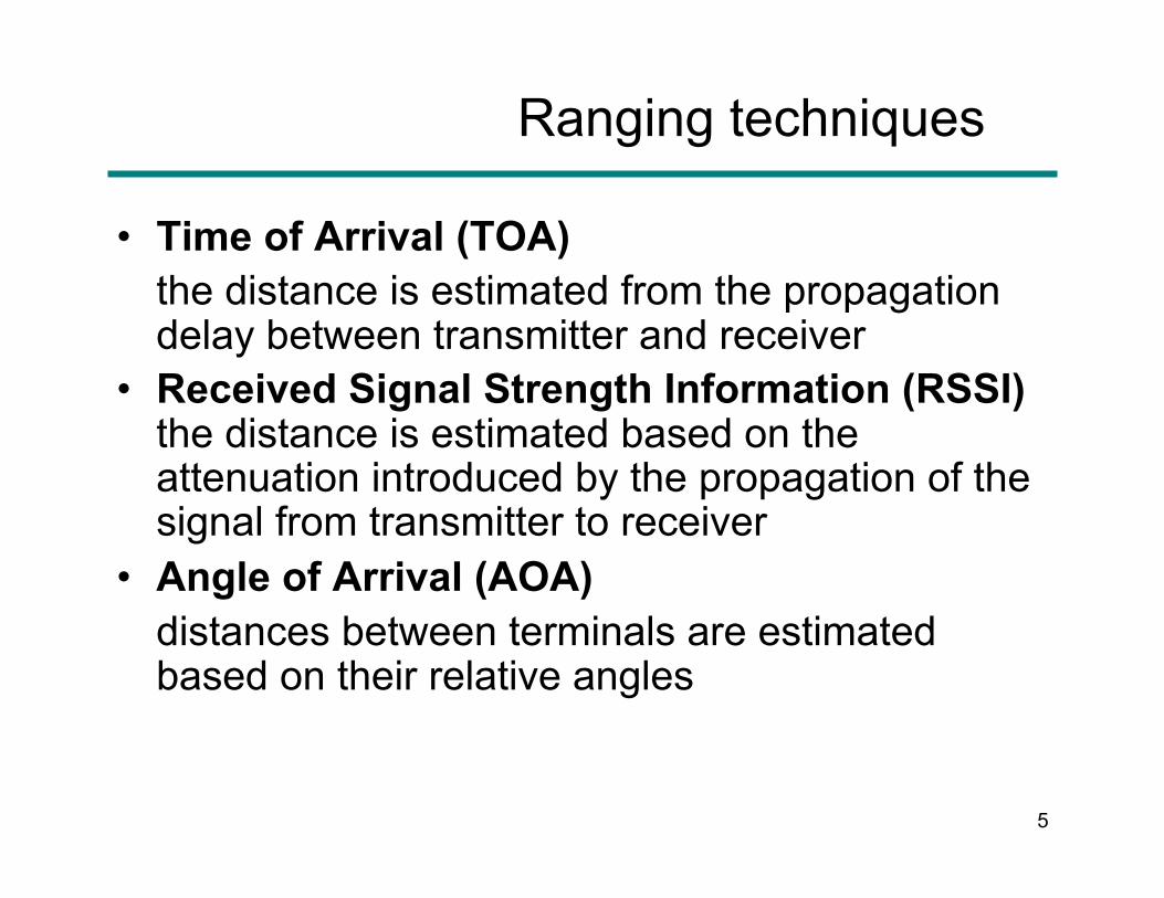
Ranging techniques
• Time of Arrival (TOA) the distance is estimated from the propagation delay between transmitter and receiver
• Received Signal Strength Information (RSSI) the distance is estimated based on the attenuation introduced by the propagation of the signal from transmitter to receiver
• Angle of Arrival (AOA) distances between terminals are estimated based on their relative angles
6
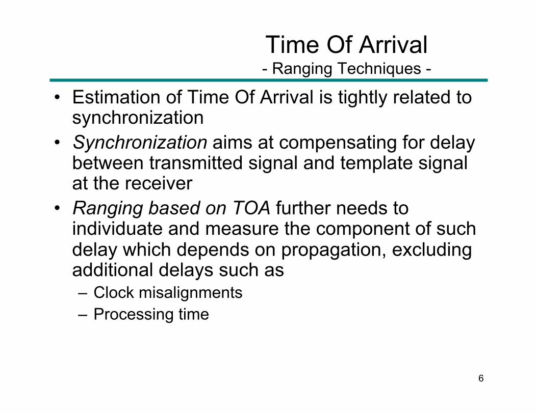
Time Of Arrival - Ranging Techniques -
• Estimation of Time Of Arrival is tightly related to synchronization
• Synchronization aims at compensating for delay between transmitted signal and template signal at the receiver
• Ranging based on TOA further needs to individuate and measure the component of such delay which depends on propagation, excluding additional delays such as – Clock misalignments – Processing time
7
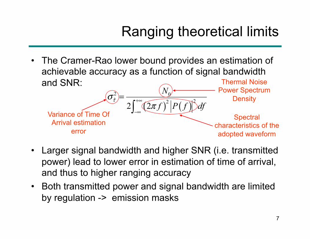
Ranging theoretical limits
• The Cramer-Rao lower bound provides an estimation of achievable accuracy as a function of signal bandwidth and SNR:
• Larger signal bandwidth and higher SNR (i.e. transmitted power) lead to lower error in estimation of time of arrival, and thus to higher ranging accuracy
• Both transmitted power and signal bandwidth are limited by regulation -> emission masks
( ) ( )2 0ˆ 222 2
N
f P f dfτσ
π+∞
−∞
=∫
Variance of Time Of Arrival estimation
error
Thermal Noise Power Spectrum
Density
Spectral characteristics of the adopted waveform
8
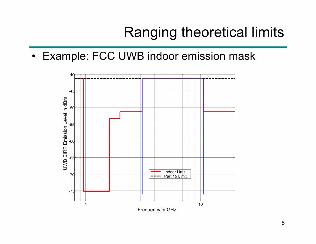
Ranging theoretical limits
• Example: FCC UWB indoor emission mask
1 10
-75
-70
-65
-60
-55
-50
-45
-40
Frequency in GHz
UW
B E
IRP
Em
issi
on L
evel
in d
Bm
Indoor Limit Part 15 Limit
9
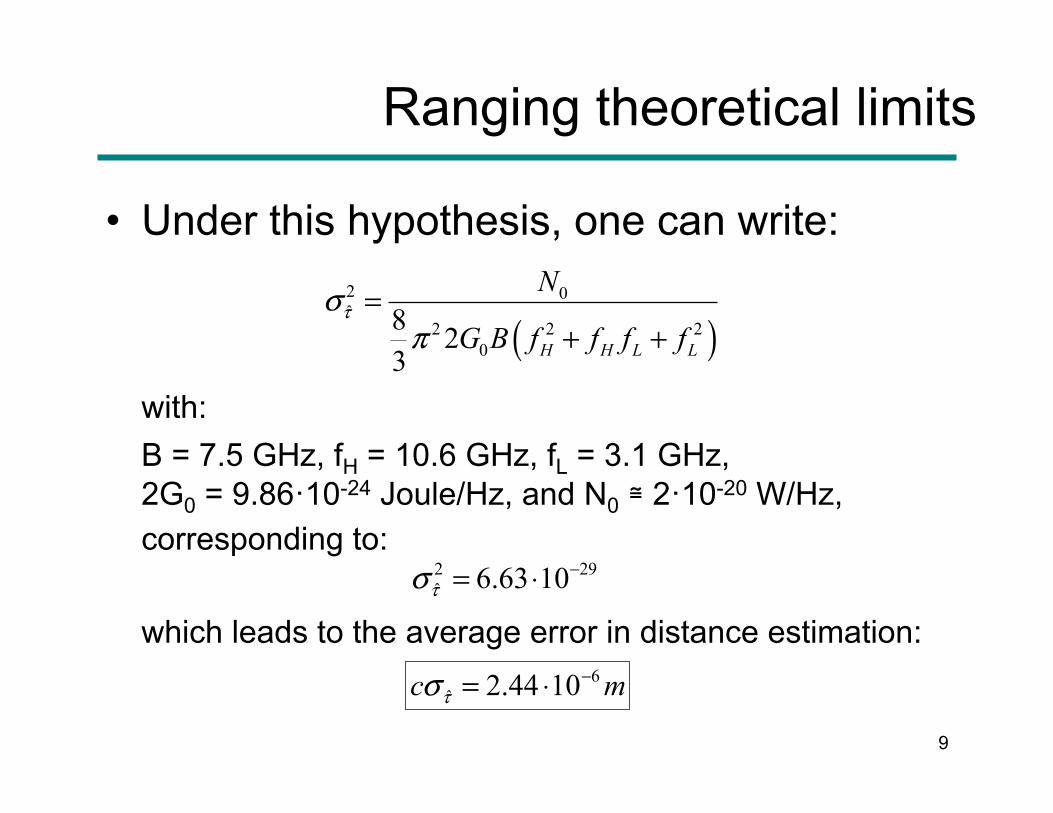
Ranging theoretical limits
• Under this hypothesis, one can write:
with: B = 7.5 GHz, fH = 10.6 GHz, fL = 3.1 GHz, 2G0 = 9.86·10-24 Joule/Hz, and N0 ≅ 2·10-20 W/Hz, corresponding to:
which leads to the average error in distance estimation:
( )2 0ˆ
2 2 20
8 23 H H L L
N
G B f f f fτσ
π=
+ +
2 29ˆ 6.63 10τσ
−= ⋅
6ˆ 2.44 10c mτσ
−= ⋅
10
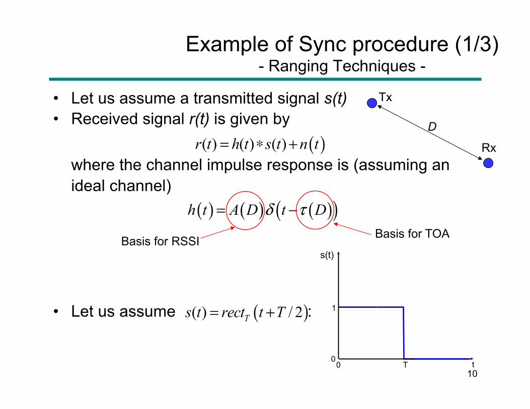
• Let us assume a transmitted signal s(t) • Received signal r(t) is given by
where the channel impulse response is (assuming an ideal channel)
• Let us assume :
Example of Sync procedure (1/3) - Ranging Techniques -
( )( ) ( ) ( )r t h t s t n t= ∗ +
( ) ( ) ( )( )δ τ= −h t A D t D
D
Tx
Rx
Basis for RSSI Basis for TOA
( )( ) / 2Ts t rect t T= +
0 T 0
1
t
s(t)
11
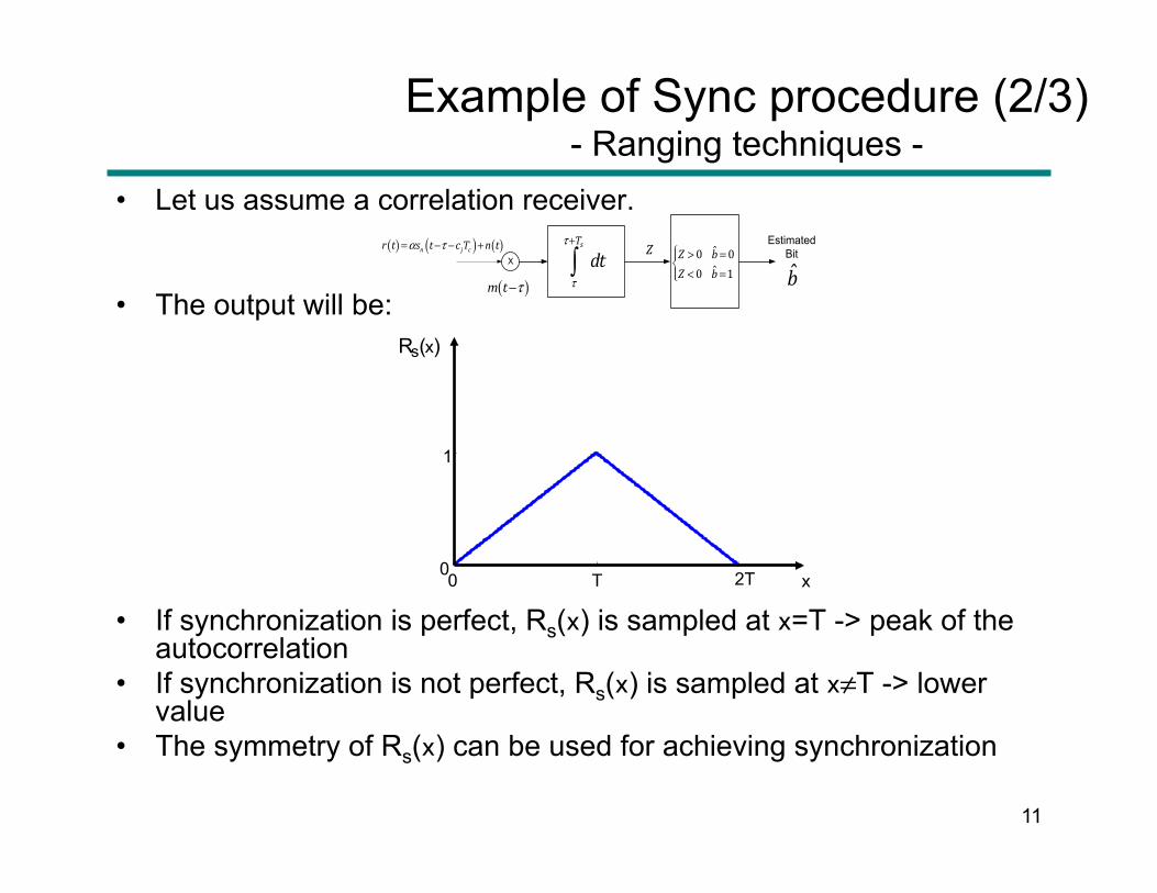
Example of Sync procedure (2/3) - Ranging techniques -
• Let us assume a correlation receiver.
• The output will be:
• If synchronization is perfect, Rs(x) is sampled at x=T -> peak of the autocorrelation
• If synchronization is not perfect, Rs(x) is sampled at x≠T -> lower value
• The symmetry of Rs(x) can be used for achieving synchronization
0 T 2T 0
1
x
R s ( x )
X
sT
dtτ
τ
+
∫( )m t τ−
Z( ) ( ) ( )n j cr t s t c T n tα τ= − − +
b̂ˆ0 0ˆ0 1
Z bZ b
⎧ > =⎪⎨
< =⎪⎩
EstimatedBit
12
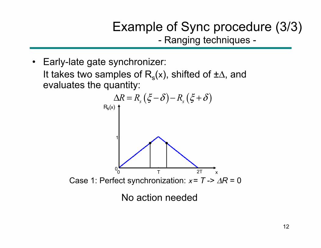
Example of Sync procedure (3/3) - Ranging techniques -
• Early-late gate synchronizer: It takes two samples of Rs(x), shifted of ±Δ, and evaluates the quantity:
0 T 2T 0
1
x
R s ( x ) ( ) ( )s sR R Rξ δ ξ δΔ = − − +
Case 1: Perfect synchronization: x = T -> ΔR = 0
No action needed
13
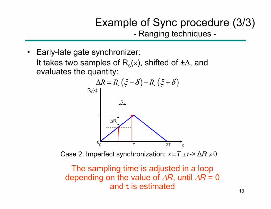
Example of Sync procedure (3/3) - Ranging techniques -
• Early-late gate synchronizer: It takes two samples of Rs(x), shifted of ±Δ, and evaluates the quantity:
0 T 2T 0
1
x
R s ( x ) ( ) ( )s sR R Rξ δ ξ δΔ = − − +
Case 2: Imperfect synchronization: x = T ± t -> ΔR ≠ 0
The sampling time is adjusted in a loop depending on the value of ΔR, until ΔR = 0
and t is estimated
ΔR
t
14
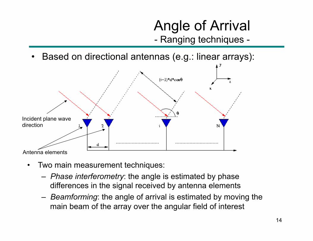
Angle of Arrival - Ranging techniques -
• Based on directional antennas (e.g.: linear arrays):
Antenna elements
Incident plane wave direction
• Two main measurement techniques: – Phase interferometry: the angle is estimated by phase
differences in the signal received by antenna elements – Beamforming: the angle of arrival is estimated by moving the
main beam of the array over the angular field of interest

15
Angle of Arrival - Ranging techniques -
• Drawbacks: – Highly coherent receiver (all channels must
have the same effect on the received signal) – The cost of the receiver increases as the
array size increases
the number of elements required to obtain a given accuracy strongly depends on the radio environment
The size should be reduced as much as possible
BUT
16
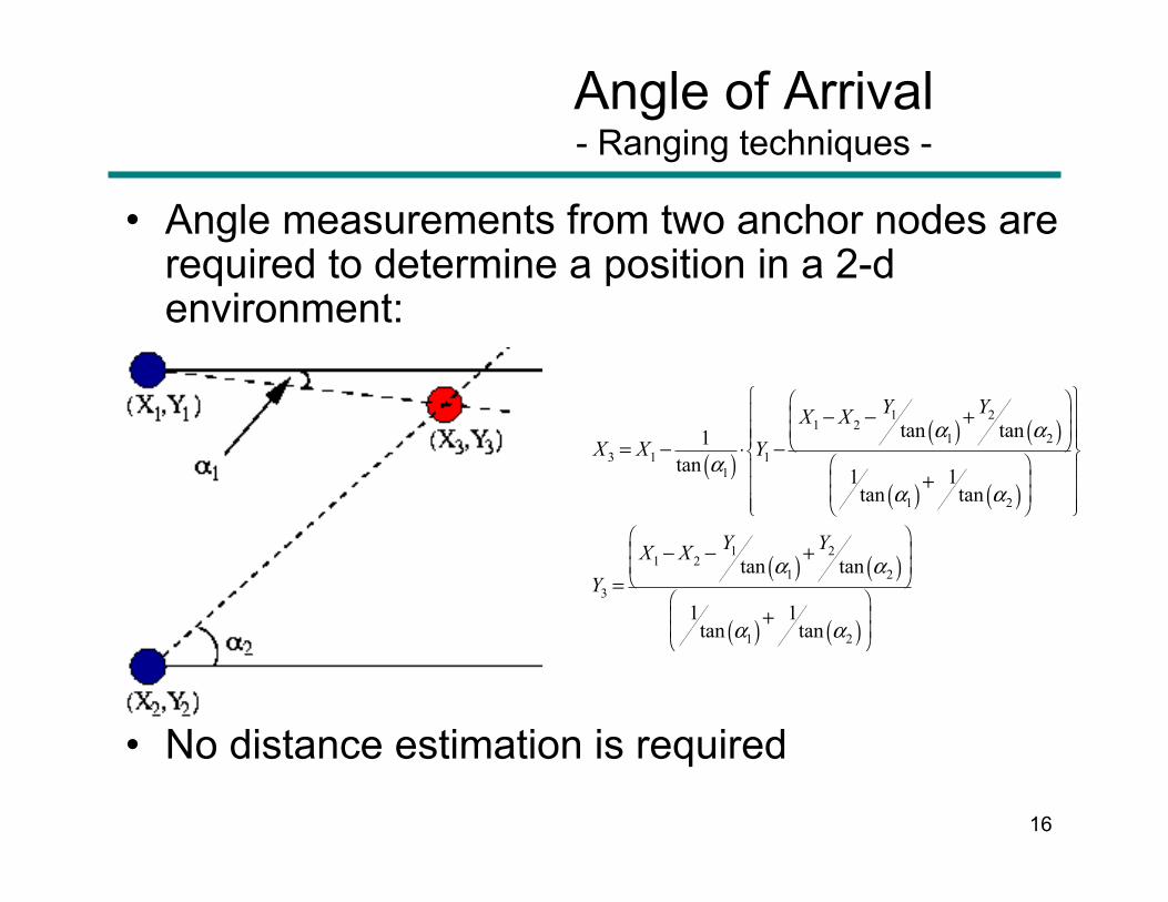
Angle of Arrival - Ranging techniques -
• Angle measurements from two anchor nodes are required to determine a position in a 2-d environment:
• No distance estimation is required
( )( ) ( )
( ) ( )
( ) ( )
( ) ( )
1 21 2
1 23 1 1
1
1 2
1 21 2
1 23
1 2
tan tan1tan 1 1
tan tan
tan tan
1 1tan tan
Y YX XX X Y
Y YX XY
α αα
α α
α α
α α
⎧ ⎫⎛ ⎞⎪ ⎪⎜ ⎟
⎜ ⎟⎪ ⎪⎪ ⎪⎝ ⎠⎨ ⎬⎛ ⎞⎪ ⎪⎜ ⎟⎪ ⎪⎜ ⎟⎪ ⎪⎝ ⎠⎩ ⎭⎛ ⎞⎜ ⎟⎜ ⎟⎝ ⎠
⎛ ⎞⎜ ⎟⎜ ⎟⎝ ⎠
− − += − ⋅ −
+
− − +=
+
17
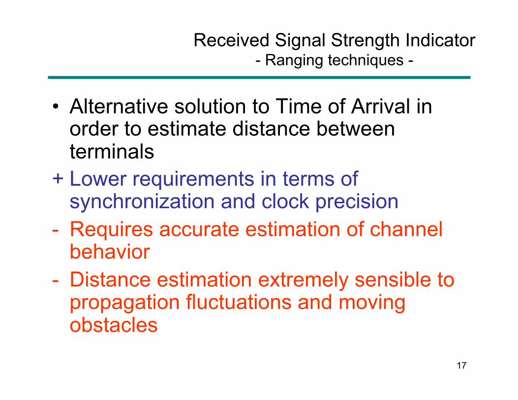
Received Signal Strength Indicator - Ranging techniques -
• Alternative solution to Time of Arrival in order to estimate distance between terminals
+ Lower requirements in terms of synchronization and clock precision
- Requires accurate estimation of channel behavior
- Distance estimation extremely sensible to propagation fluctuations and moving obstacles
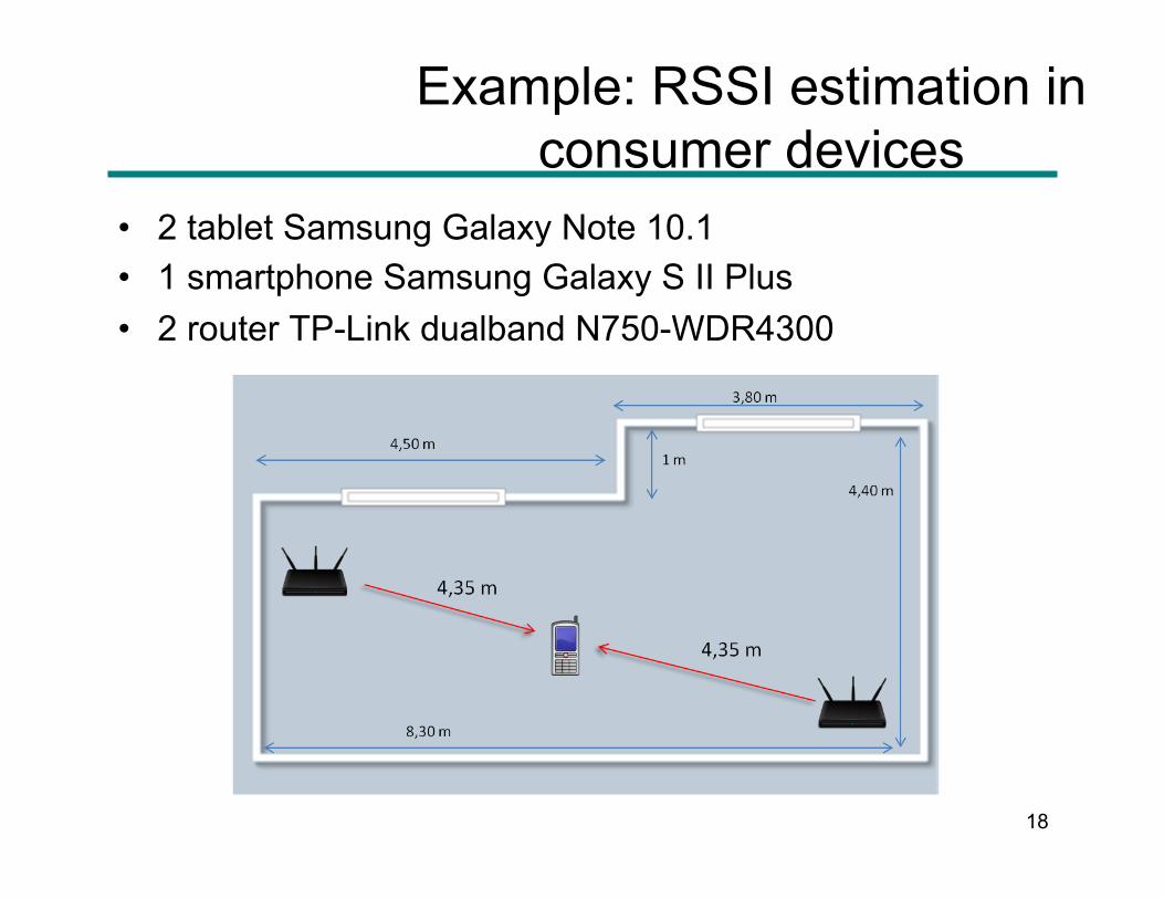
Example: RSSI estimation in consumer devices
• 2 tablet Samsung Galaxy Note 10.1 • 1 smartphone Samsung Galaxy S II Plus • 2 router TP-Link dualband N750-WDR4300
18
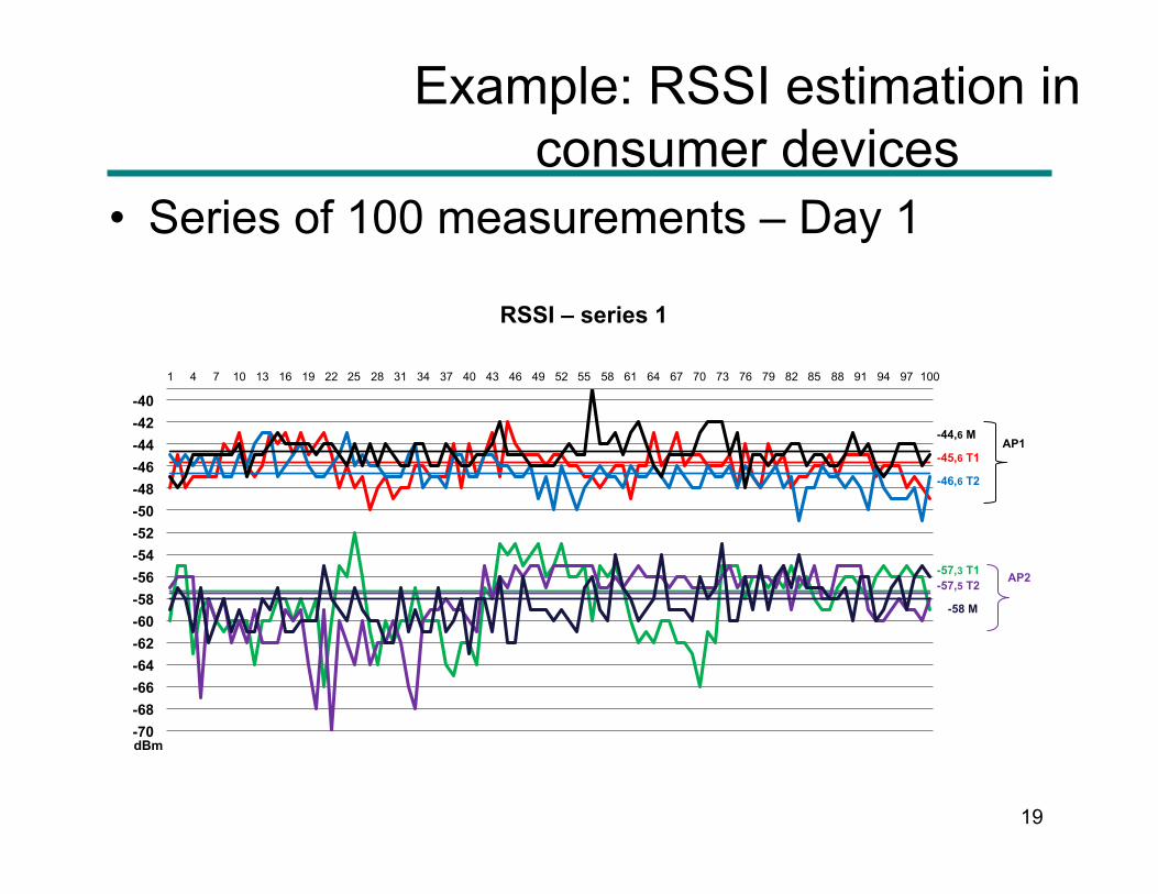
Example: RSSI estimation in consumer devices
19
• Series of 100 measurements – Day 1
-70 -68 -66 -64 -62 -60 -58 -56 -54 -52 -50 -48 -46 -44 -42 -40
1 4 7 10 13 16 19 22 25 28 31 34 37 40 43 46 49 52 55 58 61 64 67 70 73 76 79 82 85 88 91 94 97 100
RSSI – series 1
dBm
-45,6 T1
-57,3 T1
AP1 -44,6 M
-46,6 T2
-57,5 T2
-58 M
AP2
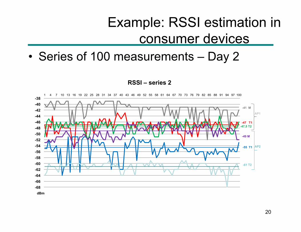
Example: RSSI estimation in consumer devices
20
-68 -66 -64 -62 -60 -58 -56 -54 -52 -50 -48 -46 -44 -42 -40 -38
1 4 7 10 13 16 19 22 25 28 31 34 37 40 43 46 49 52 55 58 61 64 67 70 73 76 79 82 85 88 91 94 97 100
RSSI – series 2
-55 T1
-47,5 T2
dBm
-47 T1
-41 M
AP2
AP1
-61 T2
-49 M
• Series of 100 measurements – Day 2
21
Summary
• Ranging – Ranging techniques
• Received Signal Strength Indicator (RSSI), Angle Of Arrival (AOA), Time Of Arrival (TOA)
– Ranging in Wireless Networks • Wi-Fi, GPS, UWB
• Positioning – Positioning techniques
• TOA, TDOA – Positioning systems
• GPS, Wi-Fi, RFID, UWB, Bluetooth – Positioning in distributed networks
• Anchor-based and anchor-less protocols – Impact on routing and navigation
• The 3D case
• Overview on RSSI-based Positioning Algorithms for WPSs - A practical implementation at the DIET Department
22
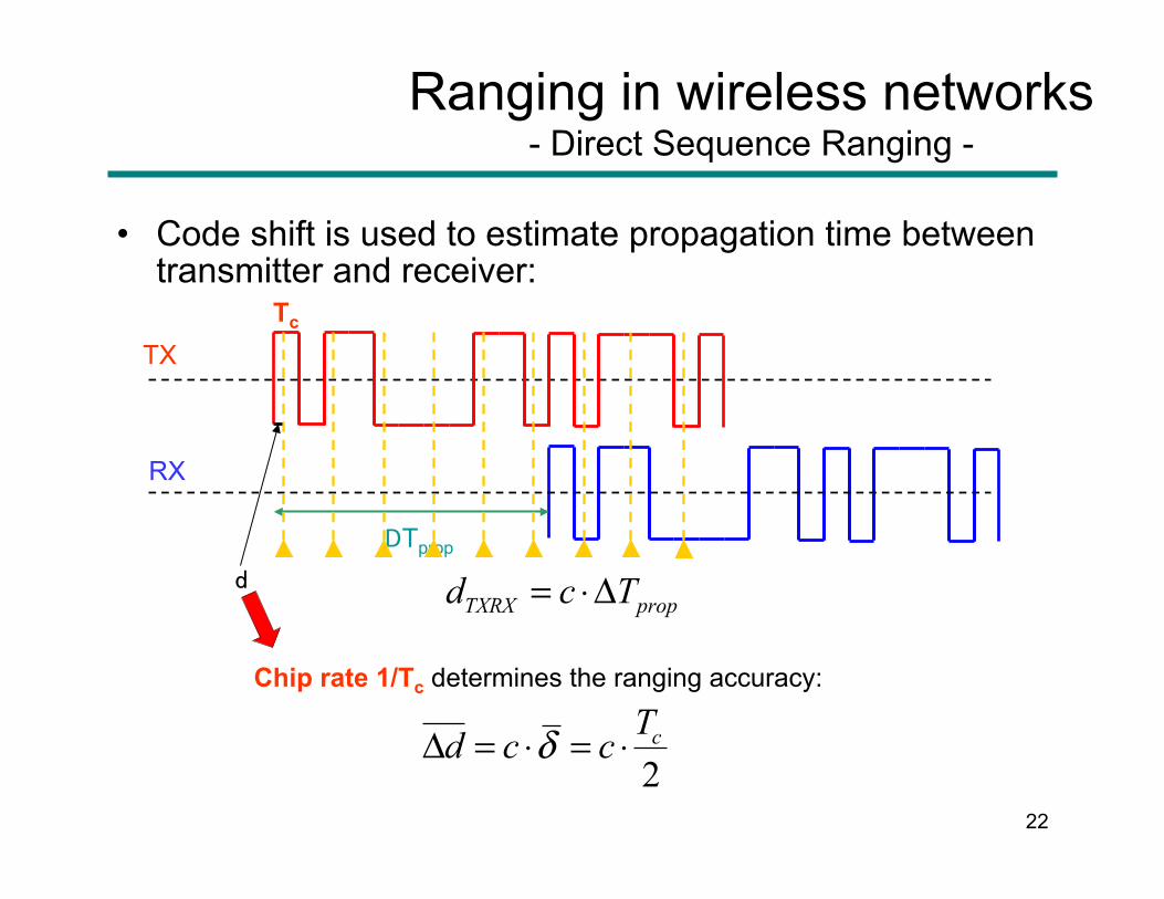
• Code shift is used to estimate propagation time between transmitter and receiver:
Ranging in wireless networks - Direct Sequence Ranging -
RX
TX
DTprop
TXRX propd c T= ⋅Δ
Chip rate 1/Tc determines the ranging accuracy:
d
Tc
2cTd c cδΔ = ⋅ = ⋅
23
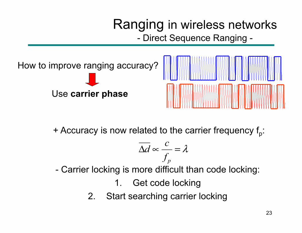
Ranging in wireless networks - Direct Sequence Ranging -
How to improve ranging accuracy?
Use carrier phase
+ Accuracy is now related to the carrier frequency fp:
- Carrier locking is more difficult than code locking: 1. Get code locking
2. Start searching carrier locking
p
cdf
λΔ ∝ =
24
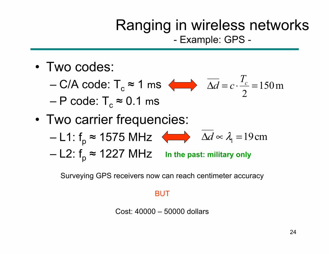
Ranging in wireless networks - Example: GPS -
• Two codes: – C/A code: Tc ≈ 1 ms – P code: Tc ≈ 0.1 ms
• Two carrier frequencies: – L1: fp ≈ 1575 MHz – L2: fp ≈ 1227 MHz
150m2cTd cΔ = ⋅ =
1 19cmd λΔ ∝ =In the past: military only
Surveying GPS receivers now can reach centimeter accuracy
BUT
Cost: 40000 – 50000 dollars
25
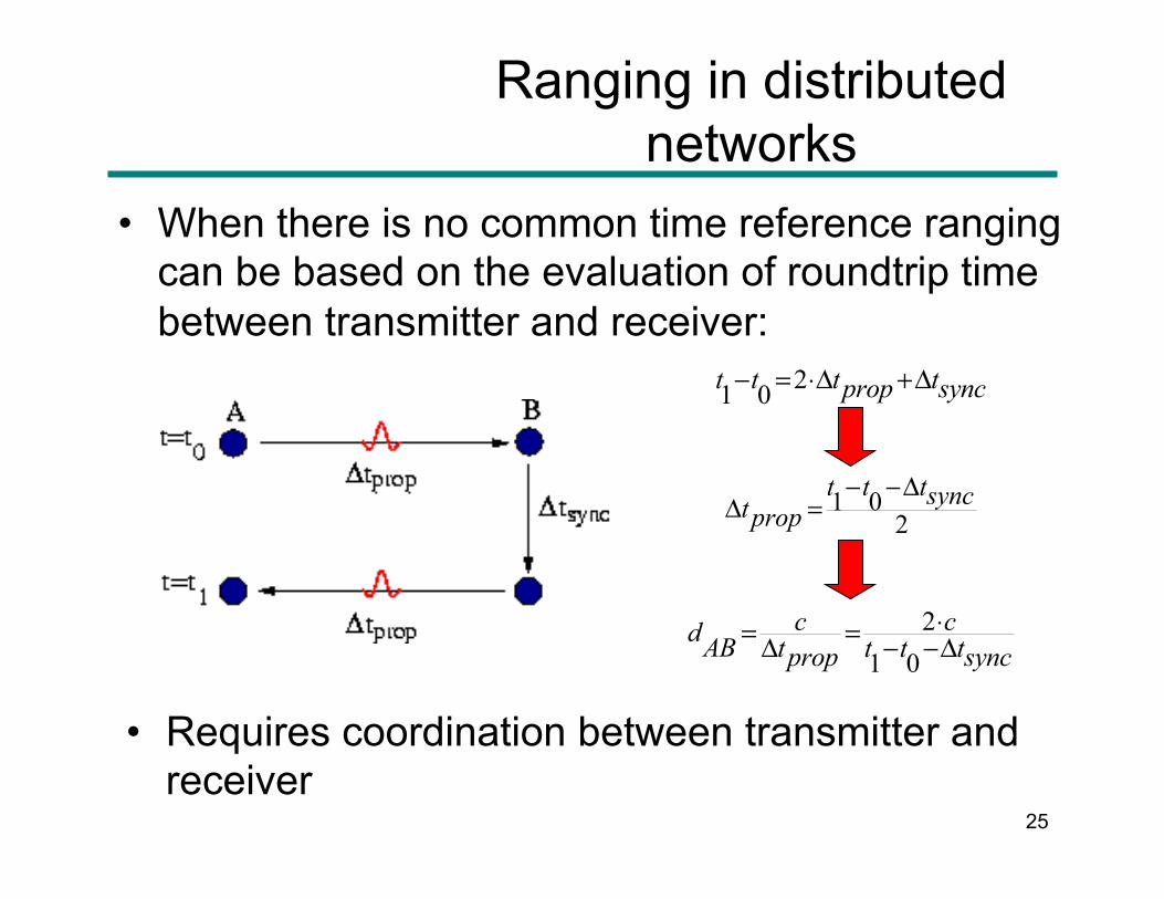
Ranging in distributed networks
• When there is no common time reference ranging can be based on the evaluation of roundtrip time between transmitter and receiver:
21 0t t t tprop sync− = ⋅Δ +Δ
1 02
t t tsynctprop− −Δ
Δ =
21 0
c cdAB t t t tprop sync⋅= =Δ − −Δ
• Requires coordination between transmitter and receiver
26
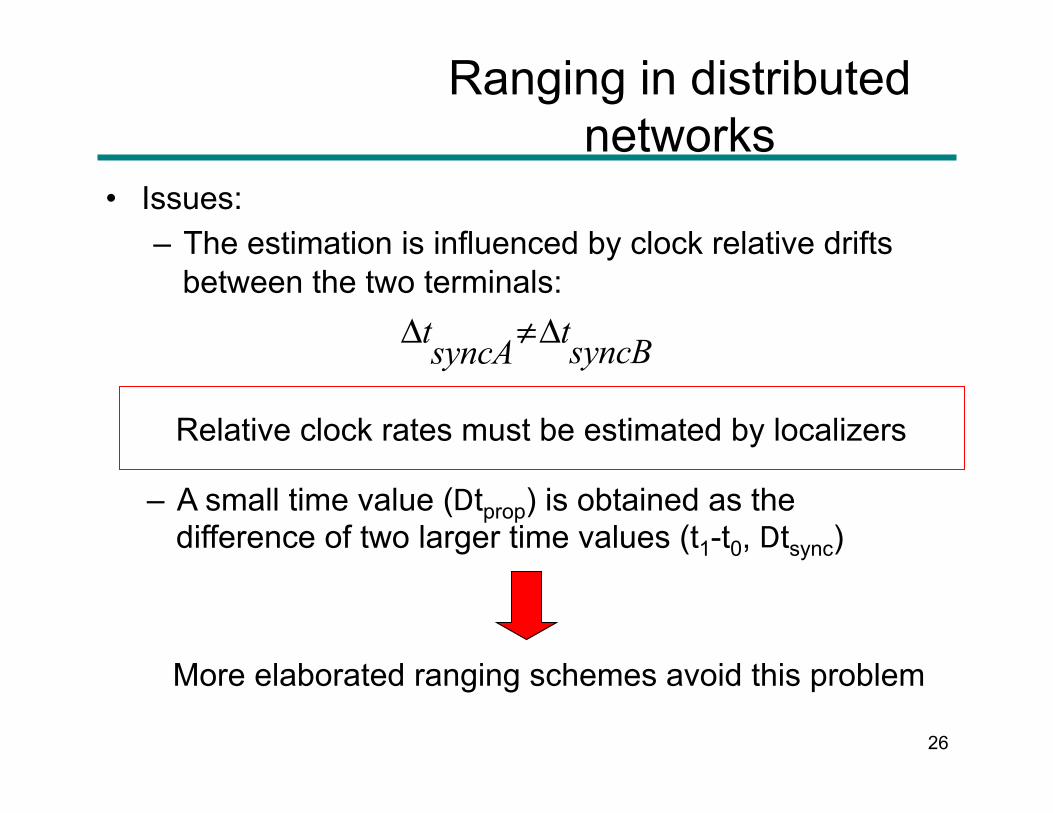
Relative clock rates must be estimated by localizers
Ranging in distributed networks
• Issues: – The estimation is influenced by clock relative drifts
between the two terminals: t tsyncBsyncAΔ ≠Δ
– A small time value (Dtprop) is obtained as the difference of two larger time values (t1-t0, Dtsync)
More elaborated ranging schemes avoid this problem

27
Summary
• Ranging – Ranging techniques
• Received Signal Strength Indicator (RSSI), Angle Of Arrival (AOA), Time Of Arrival (TOA)
– Ranging in Wireless Networks • Wi-Fi, GPS, UWB
• Positioning – Positioning techniques
• TOA, TDOA – Positioning systems
• GPS, Wi-Fi, RFID, UWB, Bluetooth – Positioning in distributed networks
• Anchor-based and anchor-less protocols – Impact on routing and navigation
• The 3D case • Overview on RSSI-based Positioning Algorithms for WPSs - A
practical implementation at the DIET Department
28
Positioning techniques
Distance information provided by ranging can be used by a node Ni in order to retrieve its own position, related to a set of reference nodes {N1,...,Nk}. This can be done by applying a positioning technique, such as: – Spherical positioning: the position of node Ni is
determined as the intersection of spheres centered in the reference nodes
– Hyperbolic positioning: the position of node Ni is determined as the intersection of spheres centered in the reference nodes
These techniques provide the same solution if distance measurements are not affected by noise
29
Spherical positioning - Positioning techniques -
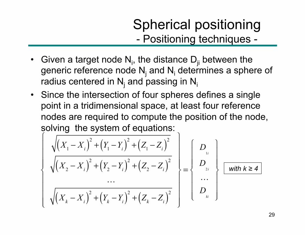
• Given a target node Ni, the distance Dji between the generic reference node Nj and Ni determines a sphere of radius centered in Nj and passing in Ni
• Since the intersection of four spheres defines a single point in a tridimensional space, at least four reference nodes are required to compute the position of the node, solving the system of equations:
X1 − Xi( )2 + Y1 −Yi( )2 + Z1 − Zi( )2
X 2 − Xi( )2 + Y2 −Yi( )2 + Z2 − Zi( )2!
Xk − Xi( )2 + Yk −Yi( )2 + Zk − Zi( )2
⎧
⎨
⎪⎪⎪⎪
⎩
⎪⎪⎪⎪
⎫
⎬
⎪⎪⎪⎪
⎭
⎪⎪⎪⎪
=
D1i
D2 i
!D
ki
⎧
⎨
⎪⎪⎪
⎩
⎪⎪⎪
⎫
⎬
⎪⎪⎪
⎭
⎪⎪⎪
with k ≥ 4
30
Spherical positioning - Positioning techniques -
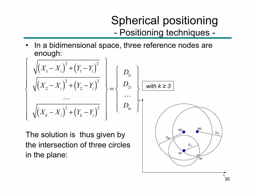
• In a bidimensional space, three reference nodes are enough:
The solution is thus given by the intersection of three circles in the plane:
X1 − Xi( )2 + Y1 −Yi( )2
X 2 − Xi( )2 + Y2 −Yi( )2!
Xk − Xi( )2 + Yk −Yi( )2
⎧
⎨
⎪⎪⎪⎪
⎩
⎪⎪⎪⎪
⎫
⎬
⎪⎪⎪⎪
⎭
⎪⎪⎪⎪
=
D1iD2i!Dki
⎧
⎨
⎪⎪
⎩
⎪⎪
⎫
⎬
⎪⎪
⎭
⎪⎪
with k ≥ 3

31
Hyperbolic positioning - Positioning techniques -
• Spherical positioning can be used only when a common time reference is available to Ni and all reference nodes {N1,...,Nk}.
• Hyperbolic positioning only requires a common time reference to be available between the reference nodes, and compensates for an unknown delay δ between the common time reference and the time reference of target node Ni by working in time differences:
• In conditions of perfect distance measurements, hyperbolic positioning leads to the same result of spherical positioning
• It can be shown however that ranging errors have a stronger effect on hyperbolic positioning
( ) ( ) ( )( ) ( )( )1 1 1ni ni nin i n i n iD D c c cτ δ τ δ τ τ− − −− = + − + = −
Unknown delay

32
Hyperbolic positioning - Positioning techniques -
• Given a target node Ni its position in a tridimensional space is determined as the intersection of hyperboloids in space, as described by the following equations:
X 2 − Xi( )2 + Y2 −Yi( )2 + Z2 − Zi( )2 − X1 − Xi( )2 + Y1 −Yi( )2 + Z1 − Zi( )2
X 3 − Xi( )2 + Y3 −Yi( )2 + Z3 − Zi( )2 − X 2 − Xi( )2 + Y2 −Yi( )2 + Z2 − Zi( )2!
Xk − Xi( )2 + Yk −Yi( )2 + Zk − Zi( )2 − Xk−1 − Xi( )2 + Yk−1 −Yi( )2 + Zk−1 − Zi( )2
⎧
⎨
⎪⎪⎪
⎩
⎪⎪⎪
⎫
⎬
⎪⎪⎪
⎭
⎪⎪⎪
=
=
D2 i − D1iD3i − D2 i
!Dki − D( k−1) i
⎧
⎨⎪⎪
⎩⎪⎪
⎫
⎬⎪⎪
⎭⎪⎪
with k ≥ 4
33
Hyperbolic positioning - Positioning techniques -
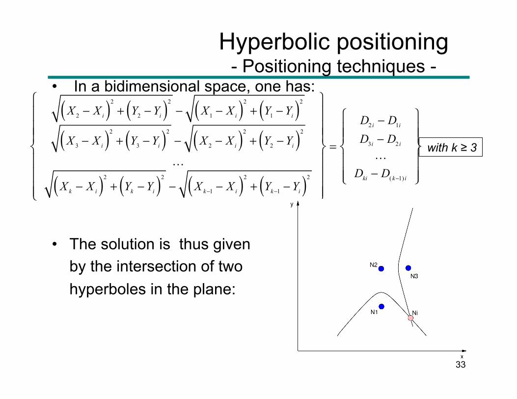
• In a bidimensional space, one has:
• The solution is thus given by the intersection of two hyperboles in the plane:
X 2 − Xi( )2 + Y2 −Yi( )2 − X1 − Xi( )2 + Y1 −Yi( )2
X 3 − Xi( )2 + Y3 −Yi( )2 − X 2 − Xi( )2 + Y2 −Yi( )2!
Xk − Xi( )2 + Yk −Yi( )2 − Xk−1 − Xi( )2 + Yk−1 −Yi( )2
⎧
⎨
⎪⎪⎪
⎩
⎪⎪⎪
⎫
⎬
⎪⎪⎪
⎭
⎪⎪⎪
=
D2 i − D1iD3i − D2 i
!Dki − D( k−1) i
⎧
⎨⎪⎪
⎩⎪⎪
⎫
⎬⎪⎪
⎭⎪⎪
with k ≥ 3

34
• In presence of ranging errors analytical solutions provided by spherical and hyperbolic positions may not exist:
• Position must be derived by means of minimization methods (e.g. Least Square Errors)
• Error in position estimation can be reduced by increasing the number of observations
Effect of ranging errors - Positioning techniques -
Distance measurements
affected by errors
35
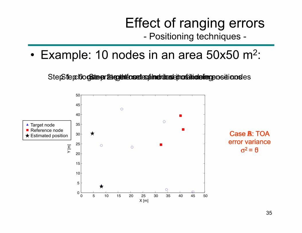
Effect of ranging errors - Positioning techniques -
• Example: 10 nodes in an area 50x50 m2:
0 5 10 15 20 25 30 35 40 45 50 0 5
10 15 20 25 30 35 40 45 50
X [m]
Y [m
] Step 1: choose a target node and a set of k reference nodes
Step 0: generate the set of nodes in random positions
Step 2: perform spherical positioning
Case A: TOA error variance
σ2 = 0
0 5 10 15 20 25 30 35 40 45 50 0
5
10
15
20
25
30
35
40
45
50
X [m]
Y [m
]
Case B: TOA error variance
σ2 = 5
Target node Reference node Estimated position
36
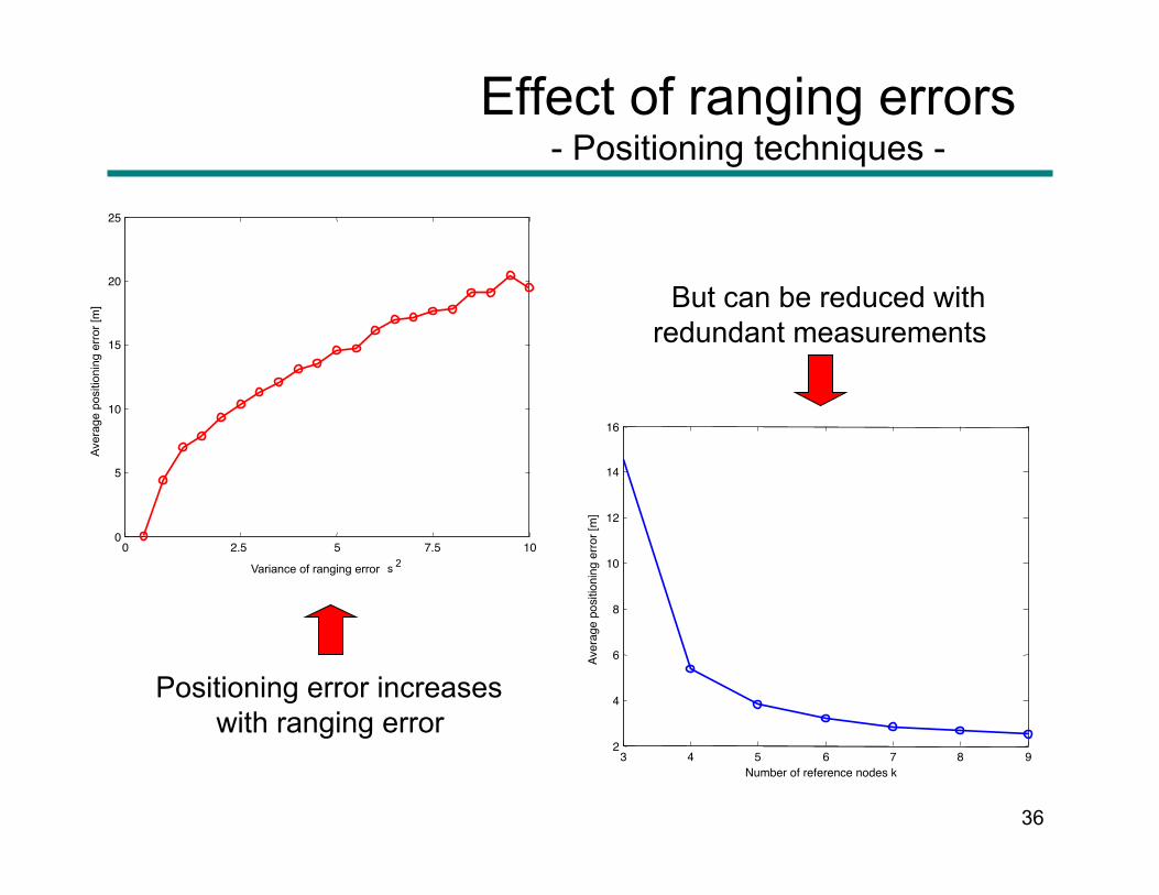
Effect of ranging errors - Positioning techniques -
Positioning error increases with ranging error
0 2.5 5 7.5 10 0
5
10
15
20
25
Variance of ranging error s 2
Aver
age
posi
tioni
ng e
rror
[m]
3 4 5 6 7 8 9 2
4
6
8
10
12
14
16
Number of reference nodes k
Aver
age
posi
tioni
ng e
rror [
m]
But can be reduced with redundant measurements
37
Summary
• Ranging – Ranging techniques
• Received Signal Strength Indicator (RSSI), Angle Of Arrival (AOA), Time Of Arrival (TOA)
– Ranging in Wireless Networks • Wi-Fi, GPS, UWB
• Positioning – Positioning techniques
• TOA, TDOA – Positioning systems
• GPS, Wi-Fi, RFID, UWB, Bluetooth – Positioning in distributed networks
• Anchor-based and anchor-less protocols – Impact on routing and navigation
• The 3D case
• Overview on RSSI-based Positioning Algorithms for WPSs - A practical implementation at the DIET Department
38
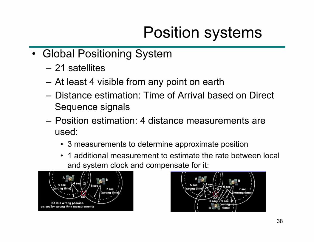
Position systems
• Global Positioning System – 21 satellites – At least 4 visible from any point on earth – Distance estimation: Time of Arrival based on Direct
Sequence signals – Position estimation: 4 distance measurements are
used: • 3 measurements to determine approximate position • 1 additional measurement to estimate the rate between local
and system clock and compensate for it:
39
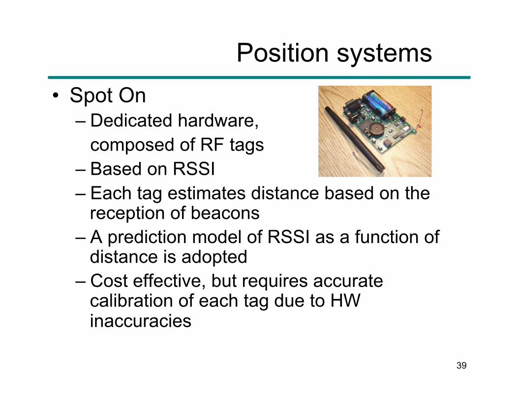
Position systems • Spot On
– Dedicated hardware, composed of RF tags
– Based on RSSI – Each tag estimates distance based on the
reception of beacons – A prediction model of RSSI as a function of
distance is adopted – Cost effective, but requires accurate
calibration of each tag due to HW inaccuracies

40
Position systems • RADAR
– Wi-Fi based positioning – Exploits fingerprinting of the target
area: a set of positions is decided a priori, and RSSI received by all Base Stations from a terminal disposed in each position is recorded
– When the position of a station must be evaluated, the system searches for the most probable combination of received power values at the base-stations and determines the closest position
– Errors in average positioning in the order of 3 - 4 meters
41
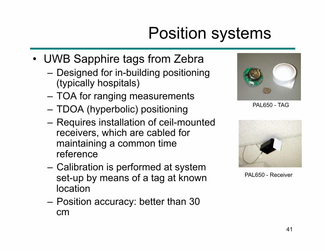
Position systems • UWB Sapphire tags from Zebra
– Designed for in-building positioning (typically hospitals)
– TOA for ranging measurements – TDOA (hyperbolic) positioning – Requires installation of ceil-mounted
receivers, which are cabled for maintaining a common time reference
– Calibration is performed at system set-up by means of a tag at known location
– Position accuracy: better than 30 cm
PAL650 - TAG
PAL650 - Receiver
42
Position systems • RFID / Bluetooth LE / iBeacons
– Based on the concept of proximity – The position of the user is associated to the position
of the closest infrastructure element – Accuracy is determined by the combination of radio
coverage and density of infrastructure element: • Lower coverage -> higher accuracy • High density required to provide reasonable area coverage
– Simple to implement, not necessarily cost effective – A system based on this concept using RFID was
implemented temporarily in the first floor of San Pietro in Vincoli in December 2012
43
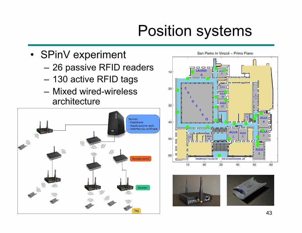
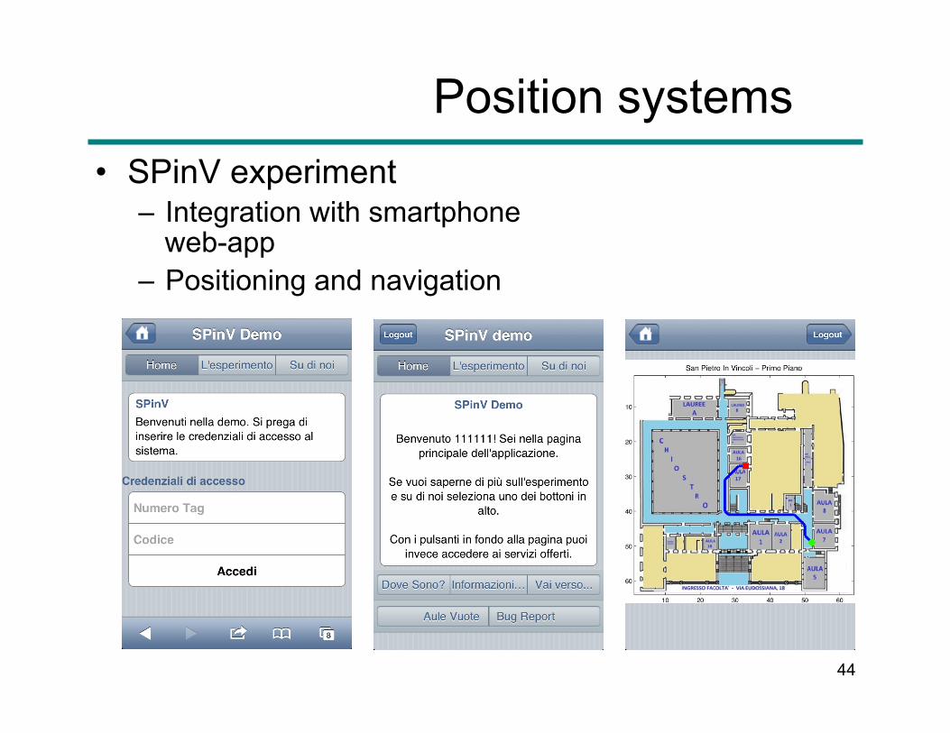
Position systems • SPinV experiment
– 26 passive RFID readers – 130 active RFID tags – Mixed wired-wireless
architecture
44
Position systems • SPinV experiment
– Integration with smartphone web-app
– Positioning and navigation
45
Summary
• Ranging – Ranging techniques
• Received Signal Strength Indicator (RSSI), Angle Of Arrival (AOA), Time Of Arrival (TOA)
– Ranging in Wireless Networks • Wi-Fi, GPS, UWB
• Positioning – Positioning techniques
• TOA, TDOA – Positioning systems
• GPS, Wi-Fi, RFID, UWB, Bluetooth – Positioning in distributed networks
• Anchor-based and anchor-less protocols – Impact on routing and navigation
• The 3D case • Overview on RSSI-based Positioning Algorithms for WPSs - A
practical implementation at the DIET Department
46
A GPS-enabled protocol - Positioning in distributed networks -
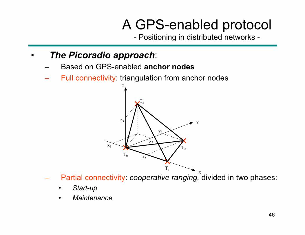
• The Picoradio approach: – Based on GPS-enabled anchor nodes – Full connectivity: triangulation from anchor nodes
– Partial connectivity: cooperative ranging, divided in two phases: • Start-up • Maintenance
T0
T1 x
y
z
T2
T3
x2
z3
x3y3
y2
47
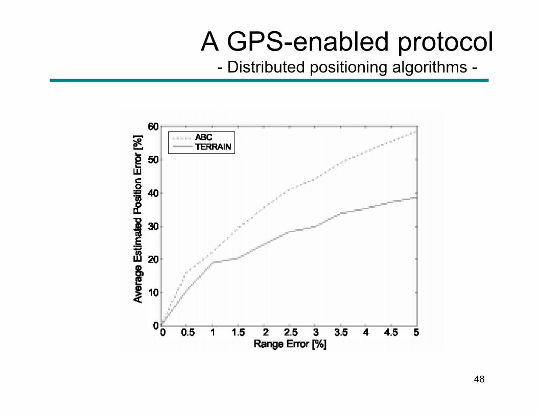
A GPS-enabled protocol - Distributed positioning algorithms -
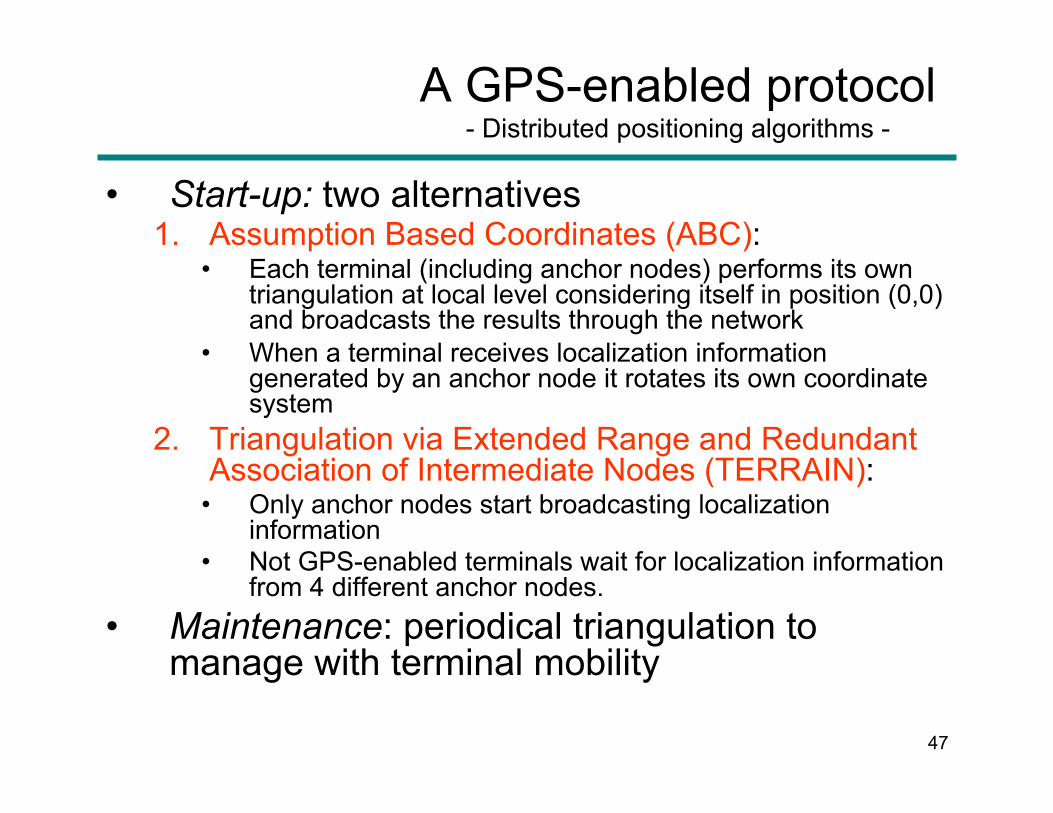
• Start-up: two alternatives 1. Assumption Based Coordinates (ABC):
• Each terminal (including anchor nodes) performs its own triangulation at local level considering itself in position (0,0) and broadcasts the results through the network
• When a terminal receives localization information generated by an anchor node it rotates its own coordinate system
2. Triangulation via Extended Range and Redundant Association of Intermediate Nodes (TERRAIN):
• Only anchor nodes start broadcasting localization information
• Not GPS-enabled terminals wait for localization information from 4 different anchor nodes.
• Maintenance: periodical triangulation to manage with terminal mobility
48
A GPS-enabled protocol - Distributed positioning algorithms -
49
A GPS-free protocol - Positioning in distributed networks -
• Self-Positioning Algorithm: – No anchor nodes – Each terminal starts its own topology
discovery – A criterion must be given to establish which
coordinate system will be adopted in the network:
• MAC address • Speed (the lower, the better) • Reliability (Available power) • ….
50
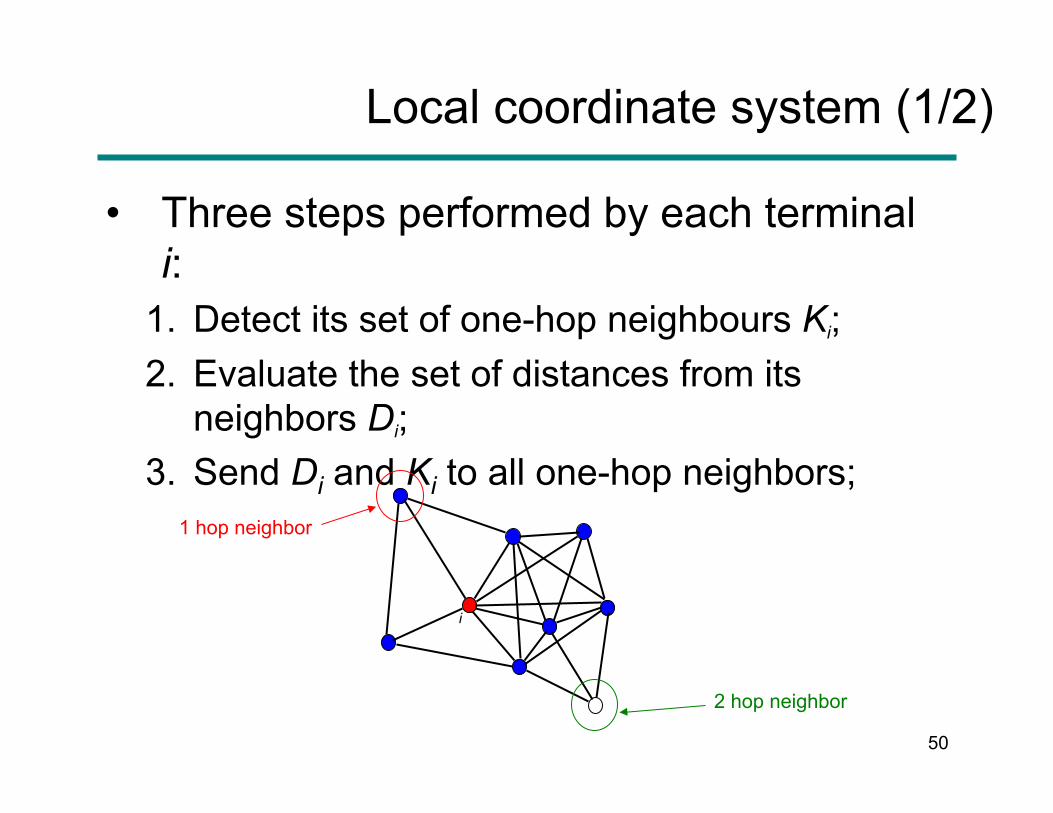
Local coordinate system (1/2)
• Three steps performed by each terminal i:
1. Detect its set of one-hop neighbours Ki; 2. Evaluate the set of distances from its
neighbors Di; 3. Send Di and Ki to all one-hop neighbors;
i
1 hop neighbor
2 hop neighbor
51
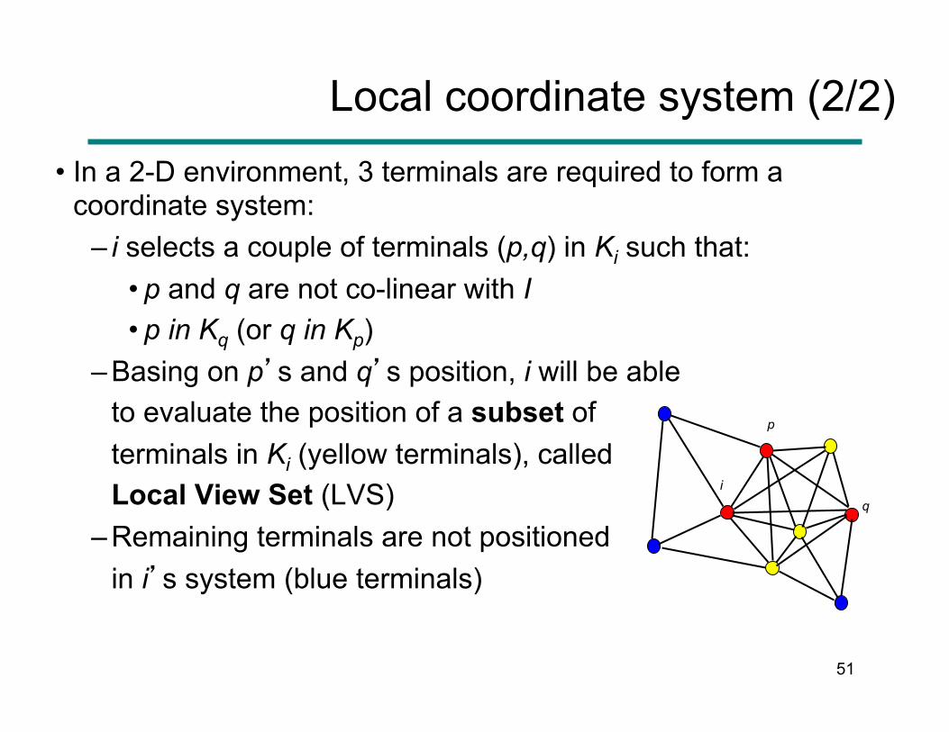
Local coordinate system (2/2) • In a 2-D environment, 3 terminals are required to form a
coordinate system: – i selects a couple of terminals (p,q) in Ki such that:
• p and q are not co-linear with I • p in Kq (or q in Kp)
– Basing on p’s and q’s position, i will be able to evaluate the position of a subset of terminals in Ki (yellow terminals), called Local View Set (LVS)
– Remaining terminals are not positioned in i’s system (blue terminals)
i
p
q

52
Network coordinate system (1/2)
• After Phase 1, terminals use different coordinate system
• Phase 2 deals with this topic, by forcing terminals to rotate and/or mirror their coordinate systems until only one remains
– Conditions for i and k to harmonize their coordinate systems: 1. i in LVSk and k in LVSi; 2. j ≠ i,k such that: j in LVSi and j in LVSk
ak aj
bi bj
i k
j
53
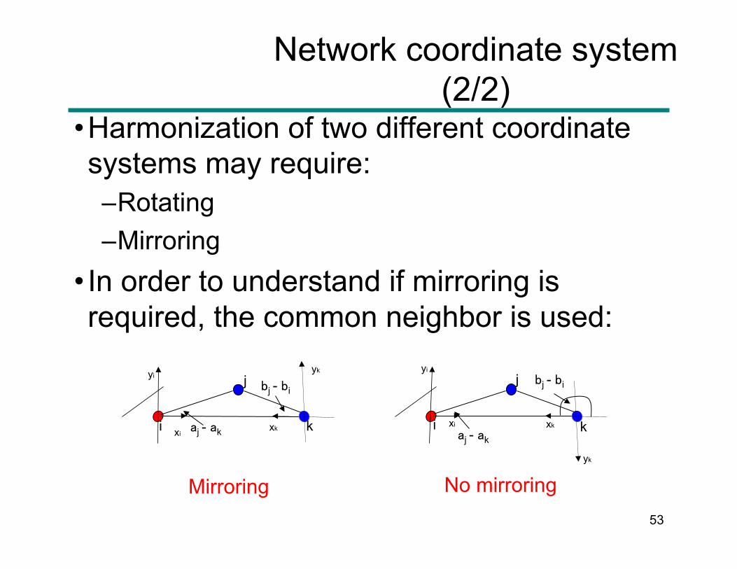
Network coordinate system (2/2)
• Harmonization of two different coordinate systems may require: – Rotating – Mirroring
• In order to understand if mirroring is required, the common neighbor is used:
aj - ak
bj - bi j
i k
bj - bi
aj - ak
j
i k
Mirroring No mirroring
xk xk
yk
yk
xi xi
yi yi
54
Algorithm definition - Open issues -
• Algorithm convergence is a serious issue with or without anchor nodes
• In real world we must take into account – Ranging errors – Communication failures – Mobility
Robustness is a key point in algorithm definition and testing phases
55
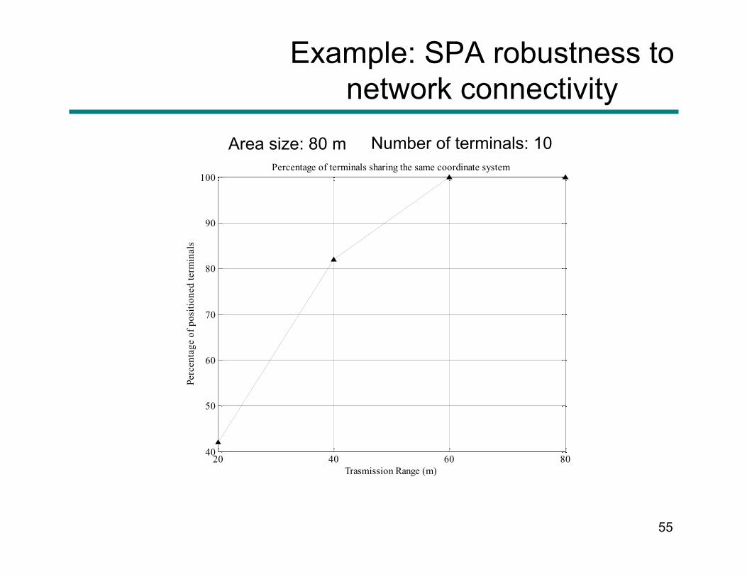
Example: SPA robustness to network connectivity
Area size: 80 m Number of terminals: 10
20 40 60 8040
50
60
70
80
90
100
Trasmission Range (m)
Perc
enta
ge o
f pos
ition
ed te
rmin
als
Percentage of terminals sharing the same coordinate system
56
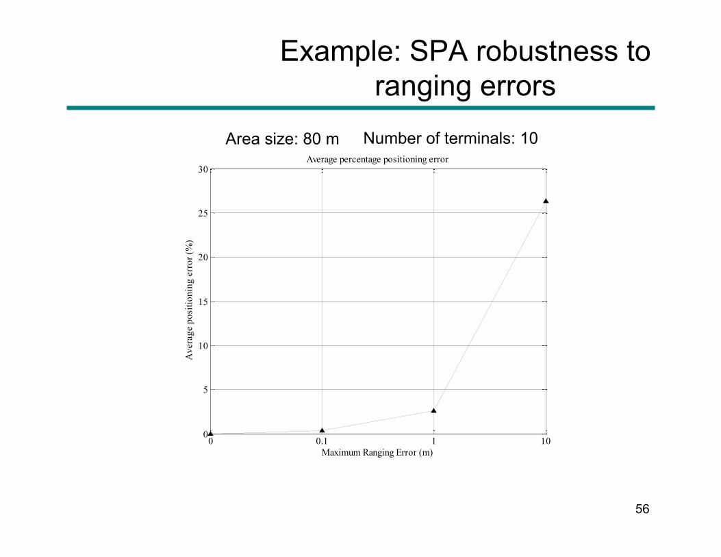
Example: SPA robustness to ranging errors
Area size: 80 m Number of terminals: 10
0 0.1 1 100
5
10
15
20
25
30
Maximum Ranging Error (m)
Ave
rage
pos
ition
ing
erro
r (%
)
Average percentage positioning error
57
Summary
• Ranging – Ranging techniques
• Received Signal Strength Indicator (RSSI), Angle Of Arrival (AOA), Time Of Arrival (TOA)
– Ranging in Wireless Networks • Wi-Fi, GPS, UWB
• Positioning – Positioning techniques
• TOA, TDOA – Positioning systems
• GPS, Wi-Fi, RFID, UWB, Bluetooth – Positioning in distributed networks
• Anchor-based and anchor-less protocols – Impact on routing and navigation
• The 3D case • Overview on RSSI-based Positioning Algorithms for WPSs - A
practical implementation at the DIET Department

58
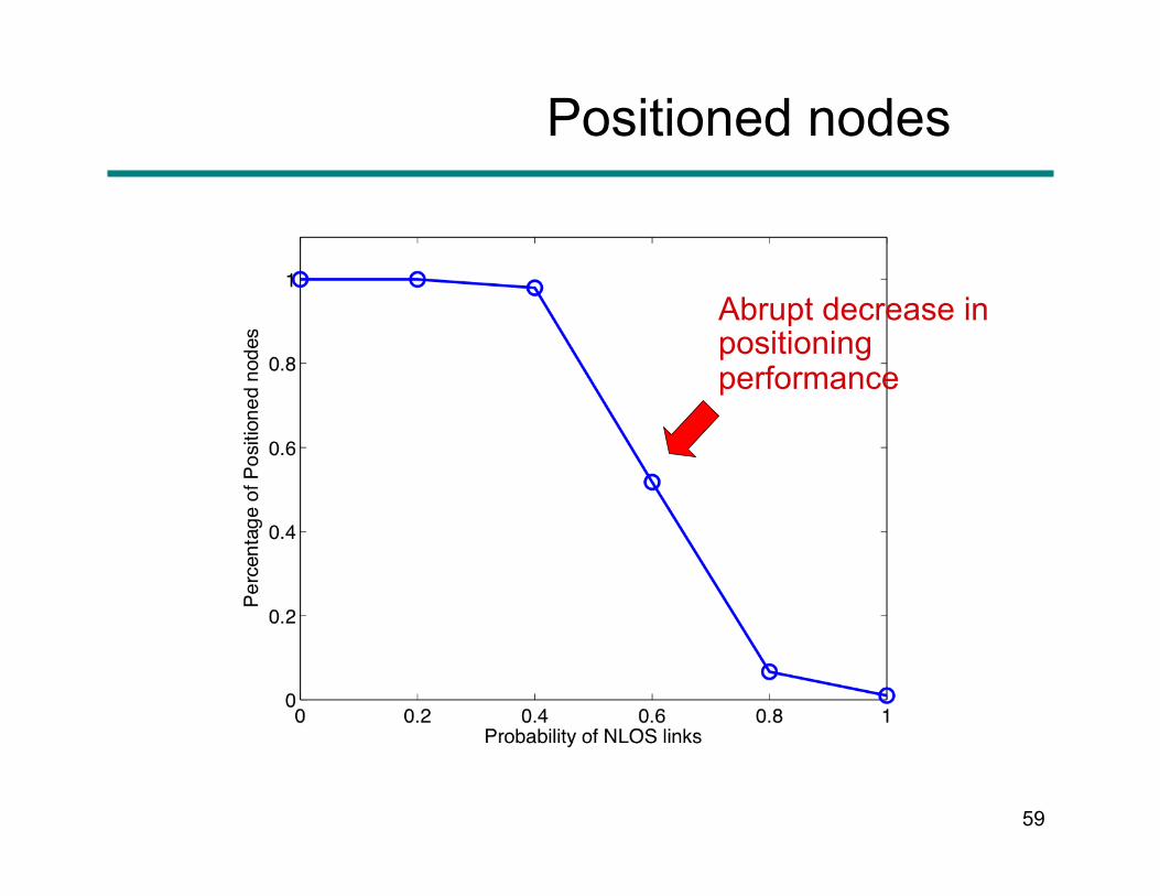
Impact of positioning accuracy on routing
• Simulation assumptions • 25 Nodes • No mobility • 150 x 150 m2
• Mixed LOS/NLOS propagation conditions – An NLOS link affects both range and ranging
accuracy • Energy consumption (Tx/Rx/Idle) and
ranging error models derived from literature • Varying connectivity scenarios, depending
on % of NLOS links
59
Positioned nodes
Abrupt decrease in positioning performance
60
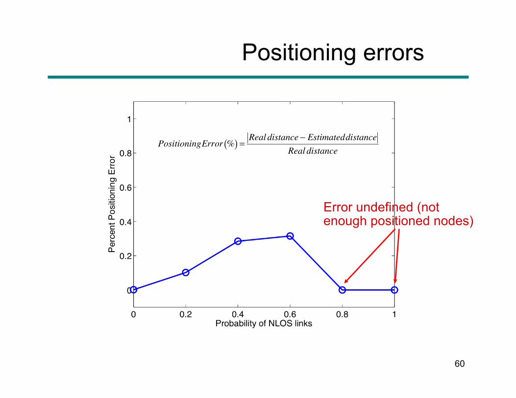
Positioning errors
Error undefined (not enough positioned nodes)
�
PositioningError %( ) =Real distance − Estimateddistance
Real distance
61
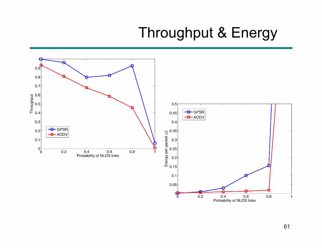
Throughput & Energy

62
Impact of positioning refresh interval
63
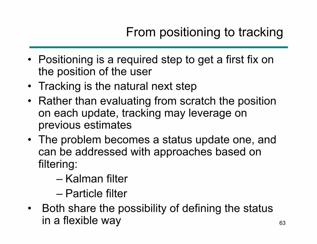
From positioning to tracking
• Positioning is a required step to get a first fix on the position of the user
• Tracking is the natural next step • Rather than evaluating from scratch the position
on each update, tracking may leverage on previous estimates
• The problem becomes a status update one, and can be addressed with approaches based on filtering:
– Kalman filter – Particle filter
• Both share the possibility of defining the status in a flexible way
64
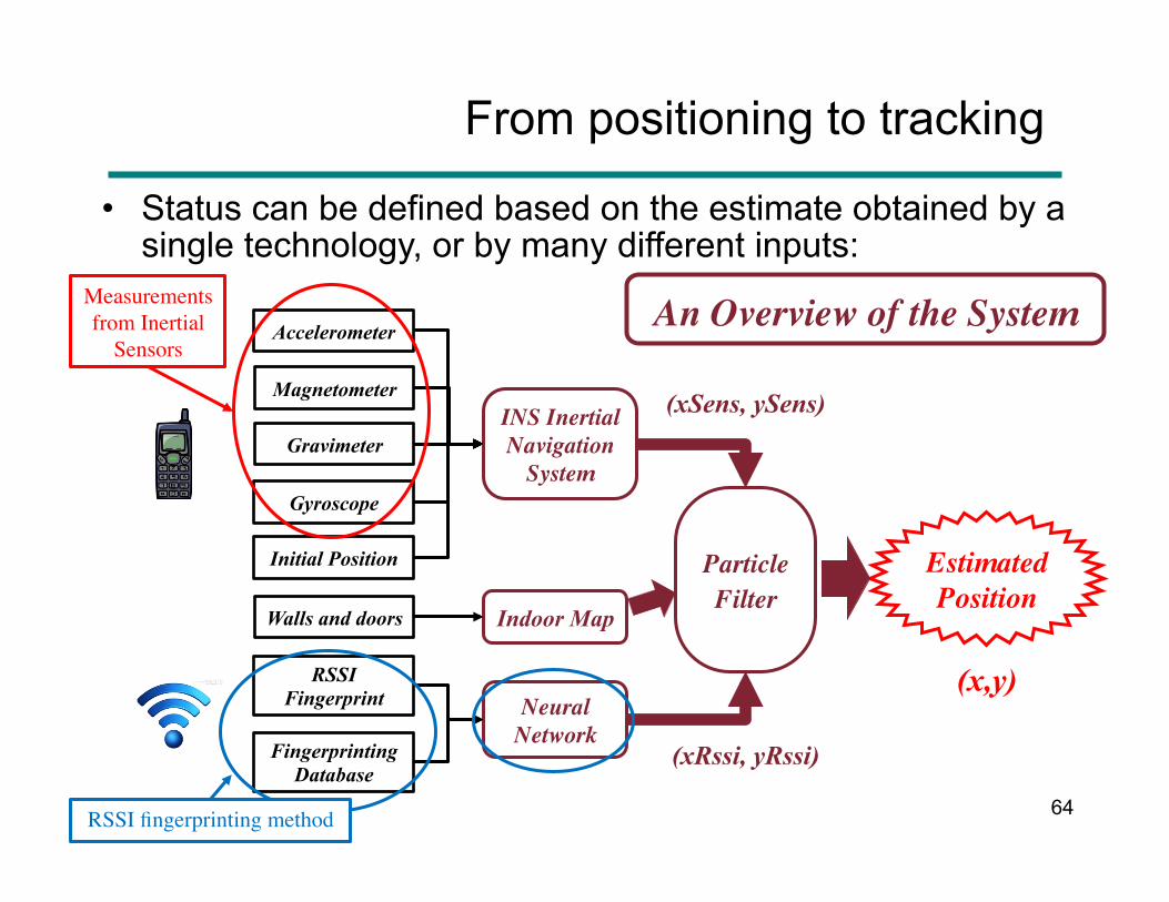
From positioning to tracking
• Status can be defined based on the estimate obtained by a single technology, or by many different inputs:
RSSI Fingerprint
Fingerprinting Database
Particle Filter
INS Inertial Navigation
System
Neural Network
Indoor Map
Estimated Position
Accelerometer
Magnetometer
Gravimeter
Gyroscope
Initial Position
Walls and doors
Measurements from Inertial
Sensors
RSSI fingerprinting method
(x,y)
(xRssi, yRssi)
(xSens, ySens)
An Overview of the System
65
Summary
• Ranging – Ranging techniques
• Received Signal Strength Indicator (RSSI), Angle Of Arrival (AOA), Time Of Arrival (TOA)
– Ranging in Wireless Networks • Wi-Fi, GPS, UWB
• Positioning – Positioning techniques
• TOA, TDOA – Positioning systems
• GPS, Wi-Fi, RFID, UWB, Bluetooth – Positioning in distributed networks
• Anchor-based and anchor-less protocols – Impact on routing and navigation
• The 3D case • Overview on RSSI-based Positioning Algorithms for WPSs - A
practical implementation at the DIET Department
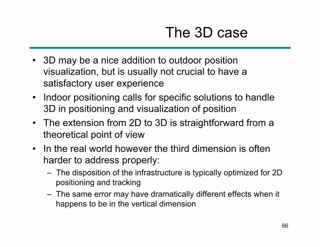
The 3D case
• 3D may be a nice addition to outdoor position visualization, but is usually not crucial to have a satisfactory user experience
• Indoor positioning calls for specific solutions to handle 3D in positioning and visualization of position
• The extension from 2D to 3D is straightforward from a theoretical point of view
• In the real world however the third dimension is often harder to address properly: – The disposition of the infrastructure is typically optimized for 2D
positioning and tracking – The same error may have dramatically different effects when it
happens to be in the vertical dimension
66
The 3D case
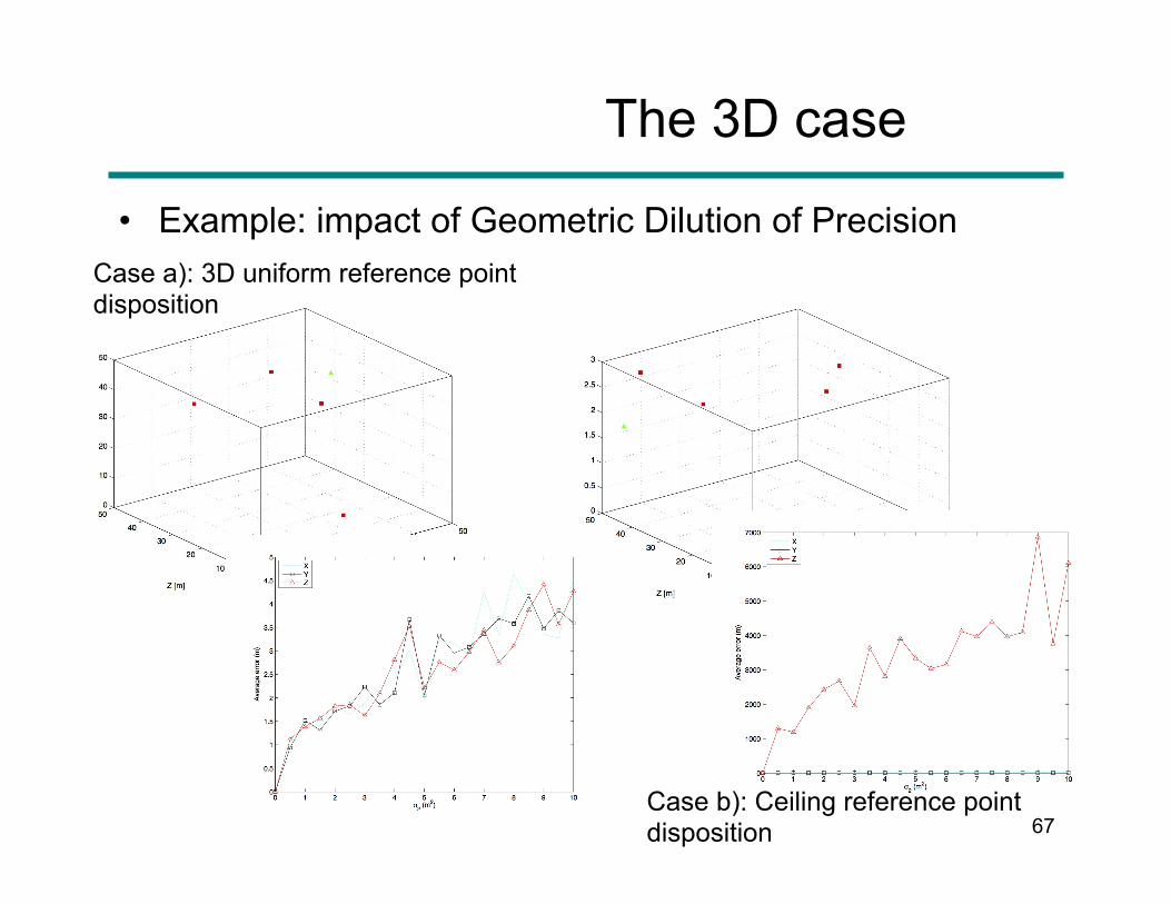
• Example: impact of Geometric Dilution of Precision
67
Case a): 3D uniform reference point disposition
Case b): Ceiling reference point disposition
The 3D case
• User mobility tracking and navigation becomes a harder problem as well
• Most technologies available for user tracking do not currently provide the same level of performance on the vertical dimension
• Examples: – Wi-Fi, due to AP typical deployment patterns – Inertial sensors / MEMS, due to difficulties in compensating drifts
due to vertical movement
• 3D tracking is also made more difficult by the need for additional coverage by the positioning infrastructure for passages between floors (e.g. stairs, elevators)
• Even simple floor detection can be a significant issue
68
The 3D case
• Visualization also requires dedicated tools in order to provide a clear, usable 3D representation of indoor environments
• Multi-floor scenarios representation in particular may become chaotic if not properly designed
• An example will be shown in the second part of the seminar, given by Giuseppe Caso
69
70
Summary
• Ranging – Ranging techniques
• Received Signal Strength Indicator (RSSI), Angle Of Arrival (AOA), Time Of Arrival (TOA)
– Ranging in Wireless Networks • Wi-Fi, GPS, UWB
• Positioning – Positioning techniques
• TOA, TDOA – Positioning systems
• GPS, Wi-Fi, RFID, UWB, Bluetooth – Positioning in distributed networks
• Anchor-based and anchor-less protocols – Impact on routing and navigation
• The 3D case • Overview on RSSI-based Positioning Algorithms for WPSs - A
practical implementation at the DIET Department
71
References • Bahl, P., and V.N. Padmanabhan, “RADAR: An In-Building RF-based User Location and Tracking
System,” Nineteenth Annual Joint Conference of the IEEE Computer and Communications Societies, Volume: 2 (March 2000), 775–784.
• Capkun, S., M. Hamdi, and J.P. Hubaux, “GPS-free positioning in mobile Ad-Hoc networks,” Hawaii International Conference On System Sciences (January 2001), 3481–3490.
• Deffenbaugh, M., J.G. Bellingham, and H. Schmidt, “The relationship between spherical and hyperbolic positioning,” MTS/IEEE OCEANS '96 ‘Prospects for the 21st Century,” Volume: 2 (September 1996), 590–595.
• Denis, B., J. Keignart, and N. Daniele, “Impact of NLOS Propagation upon Ranging Precision in UWB Systems,” IEEE Conference on UWB Systems and Technologies (November 2003), 379–383.
• Di Stefano, G., F. Graziosi, and F. Santucci, “Distributed positioning algorithm for ad-hoc networks,” International Workshop on Ultra Wideband Systems (June 2003).
• Doherty, L., K.S.J. Pister, and L. El Ghaoui, “Convex position estimation in wireless sensor networks,” Twentieth Annual Joint Conference of the IEEE Computer and Communications Societies, Volume: 3 (April 2001), 1655–1663.
• Drane, C., Positioning Systems: A Unified Approach, New York: Springer-Verlag (1992). • Drane, C., M. Macnaughtan, and C. Scott, “Positioning GSM telephones,” IEEE Communications
Magazine, Volume: 36, Issue: 4 (April 1998), 46–54, 59. • Fang, B.T., “Simple solutions for hyperbolic and related position fixes,” IEEE Transactions on
Aerospace and Electronic Systems, Volume: 26, Issue: 5 (September 1990), 748–753. • Fleming, R.A., and C.E. Kushner, “Spread Spectrum Localizers,” U.S. Patent No. 6,002,708
(1997). • Fontana, R.J., E. Richley, and J. Barney, “Commercialization of an Ultra Wideband precision
asset location system,” IEEE Conference on UWB Systems and Technologies (November 2003), 369–373.
• Getting, I.A., “Perspective/navigation-The Global Positioning System,” IEEE Spectrum, Volume: 30, Issue: 12 (December 1993), 36–38, 43–47.
• Hallberg, J., M. Nilsson, and K. Synnes, “Positioning with Bluetooth,” 10th International Conference on Telecommunications, Volume: 2 (February 2003), 954–958.

72
References • Hepsaydir, E., “Mobile Positioning in CDMA Cellular Networks,” IEEE Vehicular Technology
Conference, Volume: 2 (September 1999), 795–799. • Hightower, J., and G. Borriello, “Location systems for ubiquitous computing,” IEEE Computer, Volume:
34, Issue: 8 (August 2001), 57–66. • Hightower, J., C. Vakili, G. Borriello, and R. Want , “Design and Calibration of the SpotON Ad-Hoc
Location Sensing System,” Available at www.cs.washington.edu/homes/jeffro/pubs/ hightower2001design/hightower2001design.pdf (August 2001).
• Honkavirta, V., T. Perala, S. Ali-Loytty, R. Piché “A comparative survey of WLAN location fingerprinting methods,” 6th Workshop on Positioning, Navigation and Communication (WPNC 200), pp. 243-251, March 2009.
• Kaplan, E. (ed.), Understanding GPS: Principles and application, Norwood, MA: Artech House (1996). • Lee, J.-Y., and R.A. Scholtz, “Ranging in a dense multipath environment using an UWB radio link,”
IEEE Journal on Selected Areas in Communications, Volume: 20, Issue: 9 (December 2002), 1677–1683.
• H. Liu, H. Darabi, P. Banerjee and J. Liu, “Survey of Wireless Indoor Positioning Techniques and Systems,” IEEE Transactions on Systems, Man, and Cybernetics, Part C: Applications and Reviews, Volume 37, Issue 6 (Nov. 2007), pp. 1067 – 1080.
• Logsdon, T., The Navstar Global Positioning System, New York: Van Nostrand Reinhold (1992). • McEwan, T.E., “Short range locator system,” U.S. Patent 5,589,838 (1995). • Morgan-Owen, G.J., and G.T. Johnston, “Differential GPS positioning,” Electronics & Communication
Engineering Journal, Volume: 7, Issue: 1 (February 1995), 11–21. • Niculescu, D., and B. Nath, “Ad Hoc Positioning System (APS),” IEEE Global Telecommunications
Conference, Volume: 5 (November 2001), 2926–2931. • Niculescu, D., and B. Nath, “Ad Hoc Positioning System (APS) Using AOA,” Twenty-Second Annual
Joint Conference of the IEEE Computer and Communications Societies, Volume: 3 (March 2003), 1734–1743.
• Opshaug, G.R., and P. Enge, “Integrated GPS and UWB Navigation system: (Motivates the Necessity of Non-Interference),” IEEE Conference on UWB Systems and Technologies (May 2002), 123–127.
• Proakis, J.G., Digital Communications, 3rd Edition, New York: McGraw-Hill International Editions (1995).

73
References
• Rappaport, T.S., J.H. Reed, and B.D. Woerner, “Position location using wireless communications on highways of the future,” IEEE Communications Magazine, Volume: 34, Issue: 10 (October 1996), 33–41.
• Savarese, C., “Robust Positioning Algorithms for Distributed Ad-Hoc Wireless Sensor Networks,” Master Thesis. at http://bwrc.eecs.berkeley.edu/Research/Pico_Radio/docs/Savarese_MS_Thesis _FINAL.pdf (2002).
• Savarese, C., J.M. Rabaey, and J. Beutel, “Location in distributed ad-hoc wireless sensor networks,” IEEE International Conference on Acoustics, Speech, and Signal Processing, Volume: 4 (2001), 2037–2040.
• Shimizu, Y., and Y. Sanada, “Accuracy of Relative Distance Measurement with Ultra Wideband System,” IEEE Conference on UWB Systems and Technologies (November 2003), 374–378.
• Spirito, M.A., “On the accuracy of cellular mobile station location estimation,” IEEE Transactions on Vehicular Technology, Volume: 50, Issue: 3 (May 2001), 674–685.
• Urkowitz, H., Signal Theory and Random Processes, Dedham, MA: Artech House (1983). • GPS tutorial - http://www.trimble.com/gps/