UNIVERSITE DE MONTREAL

TASK SCHEDULING AND ACTIVITY ASSIGNMENT TO WORK SHIFTS

WITH SCHEDULE FLEXIBILITY AND EMPLOYEE PREFERENCE

SATISFACTION

MAHSA ELAHIPANAH

DEPARTEMENT DE MATHEMATIQUES ET DE GENIE INDUSTRIEL

ECOLE POLYTECHNIQUE DE MONTREAL

THESE PRESENTEE EN VUE DE L’OBTENTION

DU DIPLOME DE PHILOSOPHIÆ DOCTOR

(GENIE INDUSTRIEL)

NOVEMBER 2012

c© Mahsa Elahipanah, 2012.

UNIVERSITE DE MONTREAL

ECOLE POLYTECHNIQUE DE MONTREAL

Cette these intitulee :

TASK SCHEDULING AND ACTIVITY ASSIGNMENT TO WORK SHIFTS

WITH SCHEDULE FLEXIBILITY AND EMPLOYEE PREFERENCE

SATISFACTION

presentee par : ELAHIPANAH, Mahsa

en vue de l’obtention du diplome de : Philosophiæ Doctor

a ete dument acceptee par le jury d’examen constitue de :

M. GAMACHE Michel, Ph.D., president

M. DESAULNIERS Guy, Ph.D., membre et directeur de recherche

M. SOUMIS Francois, Ph.D., membre

M. ARTIGUES Christian, Ph.D., membre

iii

To my precious parents, for their devotion and endless support,

and my dear husband, for his love and presence

iv

ACKNOWLEDGEMENTS

I would like to acknowledge my supervisor, Professor Guy Desaulniers, who has

contributed valuable ideas, feedback and advice throughout the completion of this

research work.

This research was supported by a collaborative R&D grant offered by Kronos and

the Natural Sciences and Engineering Research Council of Canada. I wish to thank

the personnel of Kronos for their collaboration.

I must acknowledge as well the assistance given by Francois Lessard in coding the

algorithms for the last chapter of this thesis.

My thanks must go also to my colleague, Quentin Lequy, whose help in the initial

levels enabled me to develop my programming skills to fulfill this project.

I also need to thank all of those who assisted me in any respect especially Pierre

Girard, Mounira Groiez and Francine Benoıt.

I am grateful to my parents who have been my constant source of inspiration.

Without their love and support this journey would not have been made possible.

Finally, I would like to thank my husband, for his support and encouragement. I

could not have completed this effort without his assistance and tolerance.

v

RESUME

La planification des horaires de personnel travaillant sur des quarts est importante

dans le secteur des services, car elle influe directement sur les couts et la qualite du

service a la clientele. Elle constitue egalement un probleme d’optimisation combina-

toire complexe, qui necessite des outils sophistiques pour le resoudre. Cette these de

doctorat porte sur trois variantes du probleme de planification des horaires de person-

nel. Apres une breve introduction et une revue de la litterature dans les chapitres 1

et 2, les trois variantes sont etudiees dans les trois chapitres principaux.

Les deux premiers chapitres principaux abordent le probleme d’affecter des taches

et des activites aux quarts dans un environnement flexible (TSAASAF), i.e, avec la

possibilite d’ajuster les heures des quarts de travail. Dans le secteur des services, les

employes effectuent des quarts de travail et sont affectes a des activites interruptibles

et a des taches sans interruption au cours de leurs quarts de travail, a l’exclusion des

temps de pause. Chaque employe ne peut effectuer plus d’une tache ou d’une activite

au meme moment, et a droit a un seul bloc de pause au cours de son quart de travail.

Une activite est un travail avec une demande continue, exprimee comme le nombre

d’employes requis pour chaque periode de l’horizon de planification. Selon les regles

de travail, la duree d’une affectation a une activite doit etre dans un intervalle donne.

Chaque tache a une duree fixe et doit etre executee une seule fois par un seul employe

qualifie, dans une fenetre de temps specifiee.

Les quarts de travail des employes reguliers sont souvent construits quelques se-

maines avant le debut des operations, lorsque les demandes des activites et des taches

sont incertaines. Quelques jours avant les operations, lorsque des precisions sur les

demandes sont obtenues, les horaires planifies peuvent etre legerement modifies, et

afin de satisfaire la demande, des employes temporaires peuvent etre programmes. Les

modifications possibles pour les quarts de travail sont les prolongations des quarts et

les deplacements des pauses-repas.

Dans le chapitre 3, nous nous interessons a une version simple du probleme TSAA-

SAF. Le probleme d’affecter des activites dans les quarts de travail flexibles (AAFF)

consiste a attribuer uniquement les activites aux quarts de travail reguliers, alors

qu’aucun employe temporaire n’est considere. Une procedure de generation de co-

lonnes heuristique, incorporee dans une procedure d’horizon fuyant, determine les

vi

quarts de travail finaux, et leur attribue des activites. Les resultats obtenus sur des

instances generees aleatoirement sont rapportes pour evaluer la validite de la methode

de resolution proposee. Les instances generees sont regroupees dans deux classes de

petite taille et une troisieme de taille moyenne. La comparaison du nombre de sous-

couvertures obtenues (la partie principale de la fonction objectif), avec et sans flexibi-

lite, montre des ameliorations de la couverture qui peuvent etre obtenues en utilisant

les options de flexibilite : le nombre de sous-couvertures est reduit, en moyenne, de

68%, 96%, et 70% dans les premiere, deuxieme et troisieme classes, respectivement.

Bien que les temps de calcul sont beaucoup plus eleves avec la methode proposee,

nous demontrons dans le chapitre 4 qu’en supprimant deliberement a l’avance les

options jugees inutiles pour les extensions des quarts de travail, il est possible de

reduire la complexite du probleme AAFF, dans l’espoir d’obtenir un meilleur temps

de calcul. D’autre part, une version complete du probleme TSAASAF est introduite

dans le chapitre 4. Celle-ci permet de resoudre le probleme d’affecter des taches et des

activites aux travailleurs temporaires et aux quarts de travail flexibles des employes

reguliers a temps plein (ATTFF). Afin de produire des solutions de bonne qualite en

des temps de calcul rapides pour les instances de grande taille, nous developpons une

methode heuristique en deux phases. Dans la premiere phase, un modele approxima-

tif de programmation en nombres entiers mixte est utilise pour suggerer des quarts

de travail temporaires et des extensions de quarts de travail reguliers, et pour plani-

fier et affecter les taches. Dans la deuxieme phase, une procedure de generation de

colonnes heuristique integree dans une procedure d’horizon fuyant decide les prolon-

gations et les heures de pause des quarts de travail reguliers, selectionne les quarts

de travail temporaires et leur assigne des activites. Cette heuristique a ete testee sur

des instances de moyenne a grande taille generees aleatoirement, pour comparer les

differentes variantes de flexibilite. Les resultats montrent que les flexibilites addition-

nelles peuvent reduire considerablement le nombre de sous-couvertures des demandes

d’activites et que les solutions peuvent etre calculees en temps raisonnables. Afin

d’evaluer la qualite des solutions, nous avons ajoute une variante qui considere toutes

les flexibilites sauf le repositionnement des pauses. Sachant que le repositionnement

des pauses n’est pas considere dans le modele approximatif de la premiere phase, pour

cette variante, la valeur de la solution de la premiere phase sert de borne inferieure

pour la solution finale de la deuxieme phase.

Dans le chapitre 5, le probleme d’affecter des activites aux quarts de travail base

vii

sur les preferences des employes (BPAA) est introduit. Nous supposons que chaque

employe fournit ses preferences sur les activites pour lesquelles il est qualifie. Nous

cherchons un outil de resolution du probleme PBAA qui, en premier lieu, vise le cout

minimum de sous-couverture et, en second lieu, assure la satisfaction maximale des

employes a l’egard de leurs preferences individuelles. Ce second objectif n’est pas

moins important que de simplement fournir les ressources suffisantes pour repondre

efficacement aux besoins des clients. En effet, un employe satisfait est plus efficace

qu’un autre qui ne l’est pas. Ainsi, la qualite du service a une grande importance

de meme que le nombre d’employes disponibles pour offrir le service dans les entre-

prises pour lesquelles conserver ses clients est un facteur cle pour la prosperite de

l’entreprise. Pour une meilleure rentabilite, les entreprises ont besoin de satisfaire

leurs clients et pour realiser cet objectif, ils doivent satisfaire leurs propres employes.

Tout d’abord, une mesure de taux de satisfaction est definie pour quantifier la satis-

faction des employes, ensuite le deuxieme objectif est defini comme la maximisation

de la moyenne des taux de satisfaction pour les employes. Les solutions qui violent

le cout minimum par un petit pourcentage, mais comprennent des affectations plus

satisfaisantes pour les employes sont egalement interessantes en ce qui concerne les

proprietes de dominance des solutions dans le cas d’un probleme avec plusieurs objec-

tifs conflictuels. Une procedure de generation de colonnes heuristique en deux phases

est proposee. Elle memorise le nombre minimum de sous-couvertures dans la premiere

phase, puis re-optimise la solution avec la deuxieme fonction objectif dans la deuxieme

phase, tout en laissant le decideur definir l’augmentation acceptable dans le nombre

minimal de sous-couvertures. Dans les deux phases, la generation de colonnes est, a

nouveau, incorporee dans une procedure d’horizon fuyant.

La capacite de cette methode a fournir un ensemble de solutions nondominees est

comparee a une methode de ponderation qui transforme le probleme en un probleme

mono-objectif avec une somme ponderee des differents objectifs. Les decideurs ont

besoin d’un outil flexible qui soit assez efficace, en pratique pour obtenir des solu-

tions dans une plage acceptable pour chaque objectif. Ainsi, ils seront en mesure de

choisir la meilleure solution qui satisfait leurs besoins variables, alors qu’il leur est

facile de modeliser leurs preferences dans les objectifs. En pratique, cette methode

est meilleure que la methode de ponderation. D’une part, il n’y a pas le difficulte de

choisir les poids comme avec la methode de ponderation. D’autre part, elle donne au

decideur plus de controle dans la recherche des solutions avec les sous-couvertures

viii

legerement au-dessus du minimum, en contrepartie de mieux satisfaire les preferences

des employes. Cependant, la resolution d’un probleme prend plus de temps de calcul

par cette methode que par la methode de ponderation. Ainsi, certaines strategies sont

appliquees pour reduire les temps de calcul de la methode proposee, mais sans succes.

D’autre part, quand les couts de sous-couverture varient d’une activite a l’autre, cette

methode s’avere meilleure. Etant donne qu’il n’y a pas de priorite entre les employes,

la methode en deux phases peut assurer un equilibre dans la satisfaction des em-

ployes en affectant des poids aux employes proportionnellement inverse a leur degre

de satisfaction a ce jour, dans chaque tranche de temps de la procedure d’horizon

fuyant.

Les principales contributions de cette these sont d’abord l’etude de trois va-

riantes du probleme d’affectation des activites aux quarts de travail, soit les problemes

AAFF, ATTFF et BPAA, qui n’ont pas encore ete abordes dans la litterature ; et,

deuxiemement, le developpement d’heuristiques de programmation mathematique so-

phistiquees, qui fournissent des solutions de bonne qualite en des temps de calcul

acceptables. Par consequent, cette recherche fournit aux industries de services des

outils efficaces pour faire face aux changements de derniere minute dans la demande

en utilisant differentes flexibilites dans le processus de planification des horaires de

personnel, reduisant les couts d’operations et les temps de planification. D’autre part,

elle introduit une ligne directrice aux entreprises, leur permettant d’integrer autant

que possible les preferences des employes dans la construction d’horaires de travail

satisfaisants, tout en gardant les couts a des niveaux minimaux.

ix

ABSTRACT

Personnel scheduling is important in the service industry, as it impacts directly the

costs and the customer service quality. It is also a complex combinatorial optimization

problem, that requires sophisticated tools for solving it. This doctoral dissertation

addresses three variants of personnel scheduling problem. After a brief introduction

and a literature review in Chapters 1 and 2, these three variants are studied in three

main chapters.

The first two main chapters address the task scheduling and activity assignment

with shift adjustments under a flexible working environment (TSAASAF). In the

service industry, the employees perform work shifts and are assigned to interruptible

activities and uninterruptible tasks during their shifts working time, excluding the

break times. Each employee can not perform more than one task or activity at a time,

and is assigned a single break during his/her work shift. An activity is a work with

continuous demand expressed as the number of employees required for each period

of the planning horizon. According to the labor rules, the duration of an assignment

to any activity should be within a given interval. Each task has a fixed duration and

should be performed by just one qualified employee within a specified time window.

The work shifts of the regular employees are often constructed a few weeks in

advance of the operations when the activity and task demands are still uncertain.

Just a few days before the operations when these demands unveil with more accuracy,

the planned schedules can be slightly modified and on-call temporary employees can

be scheduled to satisfy the demands as best as possible. As acceptable modifications,

extending the planned shifts and moving their meal breaks are considered.

In Chapter 3, we are interested in a simple version of the TSAASAF problem.

The activity assignment problem with flexible full-time shifts (AAFF) involves as-

signing only activities to the scheduled work shifts while no temporary employee is

considered. A column generation heuristic embedded into a rolling horizon procedure

determines the final shifts and assigns activities to them. Computational results ob-

tained on randomly generated instances are reported to evaluate the validity of the

proposed solution method. Generated instances are categorized in two small-sized

and one medium-sized classes. Comparing the number of undercoverings obtained

(the main part of the objective function) with and without flexibilities shows the

x

coverage improvements that can be achieved by using flexibilities: the number of un-

dercoverings is reduced, on average, by 68%, 96%, and 70% in the first, second and

third classes, respectively.

Although the computational times are much higher with the proposed method,

we show in Chapter 4 that by removing the unhelpful options for shift extensions

deliberately in advance, it is possible to reduce the complexity of AAFF problem,

in hopes of getting better computational times. Besides, a complete version of the

TSAASAF problem is introduced in Chapter 4. This version solves the task scheduling

and activity assignment to temporary and flexible regular full-time shifts (ATTFF)

problem. In order to produce good quality solutions in fast computational times for

large-sized instances, we develop a two-phase heuristic method. In the first phase, an

approximate mixed integer programming model is used to suggest temporary shifts

and extensions to regular shifts, and to schedule and assign the tasks. In the second

phase, a column generation heuristic embedded in a rolling horizon procedure de-

cides about the regular shift extensions and break placements, selects the temporary

shifts and assigns activities to them. This heuristic is tested on randomly generated

medium to large-sized instances to compare different variants of flexibility. The com-

putational results show that the additional flexibilities can yield substantial savings

in the number of activity demand undercoverings and that the solutions can be com-

puted in reasonable computational times. To assess the quality of final solutions, we

added a variant which considers all flexibilities except break repositioning. Knowing

that break movements are not considered in the first-phase approximation model, for

this variant, the value of the first-phase solution serves as a lower bound for the final

solution of the second phase.

In Chapter 5, the preference-based activity assignment to work shifts (PBAA)

problem is introduced. We suppose that each employee gives his/her preferences over

the activities he/she is skilled for. We look for a tool to solve the PBAA problem,

which in the first place, incurs the minimum undercovering cost, and in the second

place, provides the maximum employee satisfaction with respect to their individual

preferences. This latter objective is not less important than simply providing enough

resources for responding efficiently to the customers needs. In fact, a satisfied em-

ployee is more efficient than an unsatisfied one. So, the quality of service has a great

importance as well as the number of available employees to offer the service, in the

companies for which keeping customers is a key factor to a successful business. For an

xi

improved profitability, companies need to satisfy their customers and to achieve this

objective, they must satisfy their own employees. First, a satisfaction rate measure is

defined to quantify the employee satisfaction, then the second objective is defined as

the maximization of the average of satisfaction rates for employees. Solutions which

violate the minimum cost by a small percentage, but include the more satisfactory

assignments for employees are also interesting with respect to the dominance proper-

ties of the solutions for a problem with multiple conflicting objectives. A two-phase

column generation heuristic is proposed, which memorizes the minimized number of

under-coverings in the first phase, then re-optimizes the solution with the second

objective function in the second phase while letting the decision maker define the ac-

ceptable increase in the minimum number of undercoverings. In both phases, column

generation is again embedded into a rolling horizon procedure.

The capacity of this method in providing a set of nondominated solutions is com-

pared with a weighting method which transforms the problem to a single-objective

one with a weighted sum of different objectives. The decision makers need a flexible

tool which is efficient enough, in practice, to obtain solutions within the acceptable

range for each objective. Thus, they will be able to select the best solution which fits

their varying needs, while it is easy for them to interpret their preferences over the

objectives. This method outperforms the weighting method, in terms of practicality.

On the one hand, it does not have the weighting method’s difficulty to set the weights.

On the other hand, it gives the decision maker more control to find the solutions with

the undercoverings slightly above the minimum, in return for better satisfying the

employee preferences. However, it takes more computational time to solve a problem

by this method than with the weighting method. Hence, some strategies are applied

to reduce the computational time of the proposed method, which are not success-

ful. Besides, when the undercovering costs vary from one activity to the other, this

method proves to perform better. Given that there is no seniority ranking for em-

ployees, the two-phase method can provide a balance in satisfying the employees by

giving weights to the employees with inverse relationship with their satisfaction so

far, in each time slice of the rolling horizon procedure.

The main contributions of this thesis are first the study of three variants of activity

assignment to work shifts problem, as the AAFF, ATTFF and PBAA problems, not

previously studied in the literature, and second the development of state-of-the-art

mathematical programming heuristics that yield good quality solutions in acceptable

xii

computational times. Hence, this research provides the service industries with efficient

tools to deal with the last-minute changes in demands using different flexibilities in

the personnel scheduling process, reducing the operations costs and planning times.

On the other hand, it introduces a guideline to companies to incorporate as much as

possible the employees preferences in constructing satisfactory work schedules while

keeping the costs at minimum levels.

xiii

TABLE OF CONTENTS

DEDICATION . . . . . . . . . . . . . . . . . . . . . . . . . . . . . . . . . . . iii

ACKNOWLEDGEMENTS . . . . . . . . . . . . . . . . . . . . . . . . . . . . iv

RESUME . . . . . . . . . . . . . . . . . . . . . . . . . . . . . . . . . . . . . . v

ABSTRACT . . . . . . . . . . . . . . . . . . . . . . . . . . . . . . . . . . . . ix

TABLE OF CONTENTS . . . . . . . . . . . . . . . . . . . . . . . . . . . . . xiii

LIST OF TABLES . . . . . . . . . . . . . . . . . . . . . . . . . . . . . . . . . xvi

LIST OF FIGURES . . . . . . . . . . . . . . . . . . . . . . . . . . . . . . . . xvii

CHAPTER 1 INTRODUCTION . . . . . . . . . . . . . . . . . . . . . . . . 1

1.1 BASIC DEFINITIONS AND CONCEPTS . . . . . . . . . . . . . . . 1

1.1.1 Personnel Scheduling Based on Work Shifts . . . . . . . . . . 1

1.1.2 Flexible Working . . . . . . . . . . . . . . . . . . . . . . . . . 6

1.1.3 Preference Satisfaction . . . . . . . . . . . . . . . . . . . . . . 7

1.2 PROBLEM STUDIED . . . . . . . . . . . . . . . . . . . . . . . . . . 7

1.3 THESIS ORGANIZATION . . . . . . . . . . . . . . . . . . . . . . . 10

CHAPTER 2 LITERATURE REVIEW . . . . . . . . . . . . . . . . . . . . . 12

2.1 ACTIVITY/TASK ASSIGNMENT . . . . . . . . . . . . . . . . . . . 12

2.2 FLEXIBLE SHIFT SCHEDULING . . . . . . . . . . . . . . . . . . . 14

2.3 MULTI-OBJECTIVE OPTIMIZATION METHODS . . . . . . . . . 18

2.3.1 The weighted-sum method . . . . . . . . . . . . . . . . . . . . 20

2.3.2 The ε-constraint method . . . . . . . . . . . . . . . . . . . . . 23

2.4 EMPLOYEE PREFERENCE SATISFACTION . . . . . . . . . . . . 24

2.4.1 Timetabling and activity assignment to work shifts . . . . . . 24

2.4.2 Airline and rail crew scheduling . . . . . . . . . . . . . . . . . 25

2.4.3 Nurse rostering/operation room scheduling . . . . . . . . . . . 28

xiv

CHAPTER 3 A ROLLING HORIZON BRANCH-AND-PRICE HEURISTIC

FOR ACTIVITY ASSIGNMENT CONSIDERING FLEXIBLE FULL-TIME

SHIFTS . . . . . . . . . . . . . . . . . . . . . . . . . . . . . . . . . . . . . 29

3.1 ACTIVITY ASSIGNMENT PROBLEM WITH FLEXIBLE REGU-

LAR FULL-TIME SHIFTS (AAFF) . . . . . . . . . . . . . . . . . . 29

3.2 A ROLLING HORIZON BRANCH-AND-PRICE HEURISTIC . . . . 31

3.2.1 Column Generation Formulation for AAFF . . . . . . . . . . . 32

3.2.2 Rolling Horizon Procedure . . . . . . . . . . . . . . . . . . . . 35

3.2.3 Column generation heuristic . . . . . . . . . . . . . . . . . . . 38

3.3 DEFINING FLEXIBILITIES . . . . . . . . . . . . . . . . . . . . . . 45

3.4 EXPERIMENTATION . . . . . . . . . . . . . . . . . . . . . . . . . . 47

3.4.1 Test Instances . . . . . . . . . . . . . . . . . . . . . . . . . . . 47

3.4.2 Test Assumptions . . . . . . . . . . . . . . . . . . . . . . . . . 47

3.4.3 Parameters Fitting . . . . . . . . . . . . . . . . . . . . . . . . 48

3.4.4 Computational Results . . . . . . . . . . . . . . . . . . . . . . 48

3.5 CONCLUSION . . . . . . . . . . . . . . . . . . . . . . . . . . . . . . 51

CHAPTER 4 A TWO-LEVEL HEURISTIC METHOD FOR ACTIVITY/TASK

ASSIGNMENT CONSIDERING TEMPORARY AND FLEXIBLE FULL-TIME

SHIFTS . . . . . . . . . . . . . . . . . . . . . . . . . . . . . . . . . . . . . 52

4.1 TASK SCHEDULING AND ACTIVITY ASSIGNMENT TO TEM-

PORARY AND FLEXIBLE REGULAR FULL-TIME SHIFTS (AT-

TFF) . . . . . . . . . . . . . . . . . . . . . . . . . . . . . . . . . . . . 52

4.2 A TWO-PHASE HEURISTIC FOR THE ATTFF . . . . . . . . . . . 53

4.2.1 First phase . . . . . . . . . . . . . . . . . . . . . . . . . . . . 53

4.2.2 Second phase . . . . . . . . . . . . . . . . . . . . . . . . . . . 58

4.2.3 Variants . . . . . . . . . . . . . . . . . . . . . . . . . . . . . . 66

4.3 COMPUTATIONAL RESULTS . . . . . . . . . . . . . . . . . . . . . 67

4.3.1 Solution quality for the nobrkmv variant . . . . . . . . . . . . 68

4.3.2 Flexibility combinations . . . . . . . . . . . . . . . . . . . . . 70

4.3.3 Conclusion . . . . . . . . . . . . . . . . . . . . . . . . . . . . . 73

CHAPTER 5 A TWO-PHASE BRANCH-AND-PRICE HEURISTIC FOR PREF-

ERENCE BASED ACTIVITY ASSIGNMENT TO WORK SHIFTS . . . . 75

5.1 PREFERENCE-BASED ACTIVITY ASSIGNMENT (PBAA) . . . . 75

xv

5.1.1 Measuring employee satisfaction rate . . . . . . . . . . . . . . 76

5.2 MODEL FOR THE ONE-PHASE METHOD . . . . . . . . . . . . . 80

5.3 A TWO-PHASE HEURISTIC FOR THE PBAA PROBLEM . . . . . 81

5.3.1 First phase . . . . . . . . . . . . . . . . . . . . . . . . . . . . 81

5.3.2 Second phase . . . . . . . . . . . . . . . . . . . . . . . . . . . 82

5.4 RH PROCEDURE . . . . . . . . . . . . . . . . . . . . . . . . . . . . 83

5.5 BRANCHING METHOD . . . . . . . . . . . . . . . . . . . . . . . . 86

5.5.1 Column fixing . . . . . . . . . . . . . . . . . . . . . . . . . . . 86

5.5.2 Activity fixing . . . . . . . . . . . . . . . . . . . . . . . . . . . 86

5.5.3 Branching strategy selection . . . . . . . . . . . . . . . . . . . 87

5.6 ACCELERATION STRATEGIES . . . . . . . . . . . . . . . . . . . . 89

5.6.1 Exact Procedure . . . . . . . . . . . . . . . . . . . . . . . . . 89

5.6.2 Heuristic arc elimination . . . . . . . . . . . . . . . . . . . . . 93

5.7 TEST INSTANCES . . . . . . . . . . . . . . . . . . . . . . . . . . . . 94

5.8 EXPERIMENTAL PLAN . . . . . . . . . . . . . . . . . . . . . . . . 95

5.8.1 RH parameters and branching strategy . . . . . . . . . . . . . 95

5.8.2 Comparison of the one-phase and two-phase methods . . . . . 98

5.8.3 Balancing employee satisfaction rates . . . . . . . . . . . . . . 107

5.8.4 A unique undercovering cost . . . . . . . . . . . . . . . . . . . 111

5.8.5 Arc elimination . . . . . . . . . . . . . . . . . . . . . . . . . . 113

5.9 CONCLUSION . . . . . . . . . . . . . . . . . . . . . . . . . . . . . . 116

CHAPTER 6 CONCLUSION . . . . . . . . . . . . . . . . . . . . . . . . . . 118

6.1 GENERAL DISCUSSION AND CONTRIBUTIONS . . . . . . . . . 118

6.2 FUTURE WORK . . . . . . . . . . . . . . . . . . . . . . . . . . . . . 120

REFERENCES . . . . . . . . . . . . . . . . . . . . . . . . . . . . . . . . . . . 121

xvi

LIST OF TABLES

Table 3.1 Definition of arcs in subproblem of segment s ∈ S1In ∪ S2In . 42

Table 3.2 Results for 7 days, 20 shifts per day, and 5 activities (class 1) 49

Table 3.3 Results for 1 day, 50 shifts per day, and 10 activities (class 2) 49

Table 3.4 Results for 7 days, 50 shifts per day, and 7 activities (class 3) 50

Table 4.1 Definition of arcs in subproblem of segment s ∈ S1In ∪ S2In . 64

Table 4.2 Arc definition for temporary shift l ∈ L . . . . . . . . . . . . . 65

Table 4.3 Average computational results for the nobrkmv variant and dif-

ferent values of minimum assignment duration . . . . . . . . . 69

Table 4.4 Average computational results for all variants . . . . . . . . . 72

Table 5.1 Tests to set the RH parameter and branching strategy for the

second phase . . . . . . . . . . . . . . . . . . . . . . . . . . . 97

Table 5.2 Comparison of the one-phase and two-phase methods . . . . . 100

Table 5.2 (continued) . . . . . . . . . . . . . . . . . . . . . . . . . . . . 101

Table 5.3 Summary of the results for the one-phase and two-phase methods106

Table 5.4 Results for considering employee weight updates along the time

slices . . . . . . . . . . . . . . . . . . . . . . . . . . . . . . . . 109

Table 5.5 Results on instances with varying and unique undercovering

cost for activities . . . . . . . . . . . . . . . . . . . . . . . . . 112

Table 5.6 Average results for the instances with varying and unique un-

dercovering cost . . . . . . . . . . . . . . . . . . . . . . . . . . 112

Table 5.7 Results of the two-phase method variants . . . . . . . . . . . . 115

xvii

LIST OF FIGURES

Figure 1.1 Example of task scheduling and activity assignment to work shifts 5

Figure 1.2 Different cases for a flexible shift . . . . . . . . . . . . . . . . 9

Figure 2.1 Pareto-optimality . . . . . . . . . . . . . . . . . . . . . . . . . 20

Figure 2.2 Weighted-sum method with non-convex criteria space . . . . . 22

Figure 2.3 Weighted-sum method for integer programming . . . . . . . . 22

Figure 3.1 The rolling horizon procedure . . . . . . . . . . . . . . . . . . 37

Figure 3.2 Example of a network for a first segment s ∈ S1In with possible

extension . . . . . . . . . . . . . . . . . . . . . . . . . . . . . 41

Figure 5.1 Multi-objective optimization . . . . . . . . . . . . . . . . . . . 77

Figure 5.2 Example of satisfaction rates for an activity assignment . . . . 79

Figure 5.3 Shortest path network for first segment of employee 2 . . . . . 79

Figure 5.4 Criteria space for solutions of instance 1 1 . . . . . . . . . . . 102

Figure 5.5 Criteria space for solutions of instance 2 1 . . . . . . . . . . . 103

Figure 5.6 Criteria space for solutions of instance 3 1 . . . . . . . . . . . 103

Figure 5.7 Criteria space for solutions of instance 4 1 . . . . . . . . . . . 104

Figure 5.8 Criteria space for solutions of instance 5 1 . . . . . . . . . . . 104

1

CHAPTER 1

INTRODUCTION

1.1 BASIC DEFINITIONS AND CONCEPTS

Effective personnel scheduling has a great importance for service industries as a

means to remain competitive, noting their accelerating growth and the increasing

labor cost. Considering the demands, poor personnel schedules can lead to an over-

supply of workers with too much idle time, or an under-supply which will cause the

loss of business.

Personnel scheduling can be seen either as a long-term manpower decision to

determine the number of employees to be hired, known as staffing ; or as a short-

term timetabling of personnel based on work shifts considering some constraints such

as personnel preferences, time-related constraints and work rules on the assigned

schedules. In the first case, the demand for personnel is defined on a daily basis.

In the second case, it can also be defined as task/activity-based demand which is

considered in our problem as well.

1.1.1 Personnel Scheduling Based on Work Shifts

Personnel scheduling based on work shifts is decomposed into four particular as-

pects: Day-off scheduling (also known as rostering or rotating), shift scheduling, shift

assignment and task scheduling and activity assignment. When day-off scheduling,

shift scheduling and shift assignment are integrated together, we call it a tour schedul-

ing problem. These problems are briefly described in the following paragraphs.

In the literature, there have been several survey papers on personnel scheduling. In

particular, Ernst et al. (2004a) introduced a classification based on different modules,

solution approaches and application areas of personnel rostering. In another work,

Ernst et al. (2004b) presented an annotated bibliography of personnel scheduling

and rostering. Burke et al. (2004) gave a literature review on different approaches

and models applied to nurse rostering problems as well as a detailed classifications

by constraints, parameters, solution methods and criteria considered in the research

works.

2

Day-off Scheduling

In this problem, the work and rest days are decided for each employee during the

planning horizon. The aggregated schedules should satisfy the number of personnel

needed for each day or for each task planned to be done on that day in case of task-

based demand. The term ”rostering” is also used in this context, where a roster

represents the work schedule for one employee during an interval of time, which is

often a week. In ”rotating”, a roster represents the work schedule for a number of

consecutive weeks equal to the number of employees. To start, roster weeks are each

assigned to one employee. When the first week is finished the employee who has

followed the first roster week work pattern switches to the second roster week. The

other employees switch to their corresponding next roster week in the same way. So

in rotating, a roster provides a cyclic schedule for employees. The papers by Burke

et al. (2008), Moz and Pato (2007), Beddoe and Petrovic (2006), Bellanti et al. (2004),

and Valouxis and Housos (2000) deal with day-off scheduling.

Shift Scheduling

In shift scheduling problems, shifts are determined by their start and finish times

and the position of breaks (if needed to be considered). The schedules should satisfy

the personnel demand without specifying which shift is going to be assigned to which

employee. The number of shifts generated for each day is equal to the number of

personnel working on that day. There are different constraints considered in shift

scheduling problems. These may be related to the start and finish times, length or

type of the shift; or about the breaks within the shift, regarding their position, length

or number. Shift scheduling was addressed by Rekik et al. (2008), Bard et al. (2003),

Topaloglu and Ozkarahan (2003), Aykin (1996), and Bechtold and Jacobs (1990)

among others.

Shift Assignment

Shift assignment problems deal with assigning the defined shifts to employees,

based on some constraints. Each shift is only assigned to one person. Among the

related constraints there are some which represent sequence limitations or illegal shift

combinations. The others include individual limitations to work on certain shifts, or

other personnel preferences and skill requirements. The rest enforces some lower or

3

upper bounds such as the minimum rest hours between two consecutive shifts. Chu

(2007), Yeh and Lin (2007), Aickelin and Dowsland (2004), Rekik et al. (2004), Wong

and Chun (2004), Easton and Mansour (1999), and Dowsland (1998) consider shift

assignment decisions.

Tour Scheduling

Tour scheduling integrates day-off scheduling, shift scheduling and shift assign-

ment. The process involves scheduling for on and off days for the employees, as

well as assigning the scheduled shifts to their working days over the planning horizon.

This problem was studied by Chu (2007), Yeh and Lin (2007), Aickelin and Dowsland

(2004), Rekik et al. (2004), Wong and Chun (2004), Easton and Mansour (1999), and

Dowsland (1998).

Task Scheduling and Activity Assignment

When shifts are assigned to employees, task scheduling and activity assignment

determines the tasks or activities to be assigned to each working period of each shift.

The available working times in the shift span exclude the break times allocated to

the employee. Each employee can not perform more than one task or activity at a

time, but can be assigned several ones during a shift. The goal is to cover, as much as

possible, the tasks and the total personnel requirements for each activity during each

period. This problem is the center of interest of this thesis and the related literature

will be discussed further in Chapter 2.

For task scheduling and activity assignment to work shifts, as the last operational

planning level in personnel scheduling, the situation is described as follows. The em-

ployees are assigned mostly to activities (say, more than 90% of the total working

time). An activity is a work (such as operating a cash register) that has a continuous

demand (number of employees required) which may vary throughout the planning

horizon, knowing that the planning horizon is divided into consecutive periods of the

same length. The assignment of an employee to an activity can easily be interrupted

either to replace the employee by another or to reduce the offer (the employee starts

a break, ends his/her shift, or is reassigned to a different activity or task). A specific

number of tasks must also be accomplished by the employees. A task is an uninter-

ruptible piece of work with a fixed duration (spanning an integer number of periods)

4

that should begin at the beginning of a period. It needs to be performed once by a

single employee within a specified time window. For doing the task and activities,

skill requirements are also defined. As an example, in a retail store, setting a display

for an upcoming sale can be seen as a task that lasts two hours and must be accom-

plished the day before the sale starts. As opposed to an activity which requires a

given number of employees in function of the time throughout the planning horizon,

a task offers some flexibility with regards to its scheduling. Indeed, they are usually

scheduled when activity demand is low compared to the number of employees avail-

able. Often, labor rules restrict the duration of an assignment to an activity to fall

within a prescribed interval that depends on the activity itself. A minimum duration

might ensure a better quality of life for the employees and a higher productivity for

the company. A maximum duration might be mandatory for stressful activities.

An example of task scheduling and activity assignment to work shifts is illustrated

in Figure 1.1. The horizon is divided into 14 equal periods on the horizontal axis. In

each period, the demand for each type of activity A or B is equal to the height of the

corresponding block at the bottom part. The vertical axis on top holds for employees

and their shifts of work along the horizon. The position of break for each shift is

shown by the black section. The shifts are filled with activities except during their

break times. There is also a task C assigned to employee 2. The middle part shows the

two curves for coverage of each activity type resulted by the above assignments. We

say that one undercovering occurs for each employee short of the minimum number

of employees needed to perform an activity in a period. Contrarily, one overcovering

occurs for each employee in excess of the minimum number of employees needed

to perform an activity in a period. A positive amount during a period shows the

overcovering of the activity during that period, while a negative amount presents the

undercovering for that period and a zero amount shows that the demand is perfectly

satisfied. For example, for activity A during period 5 there is a lack of 1 employee,

knowing that the demand is 2 but just employee 2 is assigned activity A during this

period. So the resulted undercovering is shown as a negative 1 unit on the coverage

curve.

In general, hard constraints are requirements which originate in legislation as labor

law or union contracts. Soft constraints can be the criteria for the quality of the

schedules or personnel requests, and a weight can be used to adjust their importance.

Hard constraints must be satisfied at all costs. Soft constraints are desirable but

5

A

B A

A

BA

B

BA

B

AA

A

B AB B

A

B1

2

3

1 2 3 4 5 6 7 8 9 10 11 12 13 14

A B B A

A B C

BA

A A B

employees

1

2

3

4

coverage

B

A

demand

time

-2

-1

1

0

-2

-1

1

0

Figure 1.1 Example of task scheduling and activity assignment to work shifts

6

may be violated to generate a solution. Different objectives are considered in these

problems. Some may target the cost of schedules. Some others give more importance

to their quality; for example, aiming personnel satisfaction. Coverage of the demands

is one of the main matters of interest for most of the schedulers.

In this thesis, two special contexts are studied in parallel to the original problem

of task scheduling and activity assignment to work shifts. One is the flexible working

environment and the other is employees’ preference satisfaction. These two ideas form

three variants of the problem for each of which the models and solution methods are

developed as three axes of the present research work. The following explains the

whole idea of the two contexts, but we give the related literature review in Chapter

2.

1.1.2 Flexible Working

It is always possible for organisations to face unpredictable changes in demand

for services. Since they always want to satisfy the demand with the lowest price,

they should be able to make best use of their resources. Flexible patterns of work

maximize the available labour, among which common types include using temporary

workers, flexible working hours and overtime working.

Overtime can provide flexibility to meet labour shortages without the need to

recruit extra staff. Employees are required to work during core times, but outside

that at the beginning or end of the day, they may also be asked to work during some

flexible bands as overtime. Providing paid overtime is often less costly for employers

than recruiting and training extra staff. Employees can however become fatigued

when working excessive overtime. Sometimes a minimum duration of time is needed

to be worked before getting paid the overtime.

Employing temporary workers is another way to make the personnel scheduling

flexible to be able to respond better to the demands. It can also be an efficient way

to keep costs down when you do not need full-time cover. Temporary employees

assist to meet the demands as short-term workers in various cases such as seasonal

demand changes, regular employees sick or maternity leave. They serve as a buffer

for the ups and downs of the business cycle without affecting the core staff during

down times. They can also be the first to be laid-off in a business or economic

downturn. It is possible to obtain temporary workers from the temporary staffing

agencies. In this case, they remain the employee of the agency and don’t receive

7

benefits from the company. Besides, since the recruitment process is performed by

those agencies for a nominal fee, the companies staff time is saved. Aside from

that, the employment of temporary workers may lead to higher costs compared to

assigning overtime to full-time workers. So we should make sure that we gain enough

by using them instead. To be noted, temporary workers should not be confused with

part-timers. Part-time employees are regular employees who are not usually eligibile

for benefits such as health insurance, paid time-off or vacation days, and sick leave.

While temporary workers can work part-time or full-time, what differentiate them

from regular employees is that they do not have a commitment at the same employer

for the whole year.

On the other hand, the possibility of having flexible work or rest hours for em-

ployees helps providing more available empolyees during the periods with higher de-

mands. In this case, an employee may start/end a shift earlier/later or move the

assigned break to be available for such periods.

1.1.3 Preference Satisfaction

Besides the importance of cost reduction and customer service quality, it is also

desirable for the organisations to improve their employees’ satisfactions. Satisfied

employees are more productive, in sales for example, it is important because they

represent the company to the public. Raises or benefits improve employee content-

ment, but satisfaction is not solely linked to compensation. Providing the work-life

balance or flexible work schedules for employees are other examples causing employees’

appreciation. Besides, having the sense of control over their work schedules improves

employees contentment. The more one employee’s preferences are considered in his

work schedule, the higher would be his satisfaction level. Preferences may refer to

different subjects, including for example the type of activities or tasks to be done,

the shift hours or days off.

1.2 PROBLEM STUDIED

The problem to be addressed in the first two parts of this research is the task

scheduling and activity assignment with shift adjustments under flexible working en-

vironment (TSAASAF). In this problem, we look for better coverage for activities,

when facing the unpredictable changes in demand, by the help of a flexible schedul-

8

ing environment. Different variants of this problem may include flexible schedules,

overtime work and temporary workers. This problem is divided into two parts. The

first part which is studied in Chapter 3 is devoted only to activity assignment with

flexible schedules and overtime work; and the second one adds task scheduling and

temporary workers to that in Chapter 4.

In the activity assignment problem with flexible regular full-time shifts (AAFF),

the work and rest days for each full-time employee is already fixed for a whole month.

Also, the shifts have been constructed and assigned to the employees. These shifts

make the inputs called ”primary full-time shifts” to our problem. It means that

firstly, a set of start and finish time pairs, representing full-time work shifts for each

day, is available. Secondly, approximate working schedules with the break placements

are specified as a daily basis for each regular full-time worker one month before the

operations. There is one break with a fixed duration assigned to each shift. Then

two days to one week prior to the operations we get a better knowledge of demands

for activities. The concern then, is to assign the activities to the shifts. In order to

increase the coverage of activities, it may be required to re-schedule the shifts (without

changing the shifts’ assignments to the employees) and to change the position of

breaks. This would be possible regarding the flexibilities defined for these shifts. The

flexibilities are defined as follows: The shifts are given but are also extendible from

one end; it means that for example an eight-hour shift which normally starts at 8 am

and ends at 4 pm can be extended to start at 7 am or end at 5 pm. Another flexibility

issue is in determining the break within the shifts. It can be moved within a specified

time window, rather than being limited to start at a fixed time. Different possible

changes to a primary full-time shift by applying the above-mentioned flexibilities are

illustrated in Figure 1.2 with the following explanations:

1. The first case represents the primary shift.

2. The second case represents the break movement possibility with no extension

in the primary shift.

3. The third case represents an extension to the start of the primary shift.

4. The fourth case represents an extension to the end of the primary shift.

5. The fifth case represents the break movement possibility with an extension to

the start of the primary shift.

6. The sixth case represents the break movement possibility with an extension to

9

the end of the primary shift.

1st segment 2nd segment break

1

2

3

4

5

6

Figure 1.2 Different cases for a flexible shift

In the task scheduling and activity assignment to temporary and flexible regular

full-time shifts (ATTFF), besides the assumptions made above, there are also some

tasks to be assigned to full-time employees. Tasks should be either fulfilled for their

whole duration, or should not be assigned to anyone at all. Temporary shifts can also

be added in order to improve the coverage for activities besides the option to have

overtime for the full-time shifts. The trade-off between the incurred overtime and

temporary employees costs determines the combination of temporary shifts and the

assigned overtime to regular employees. This problem is studied in detail in Chapter

4. Hur et al. (2004) provided a case study on work schedule adjustment decisions

in case of demand uncertainty to achieve the best profit and service targets at the

same time, and investigated the influence of different factors on the efficiency of these

decisions. It is concluded that the higher proportion of part-timers used in workforce

mix may lead to higher profits in case of shortage in staff with respect to the demand

changes.

In Chapter 5, the satisfaction of employees preferences in performing the preferred

activity types is considered to be the secondary objective, after the more important

objective of minimizing the number of undercoverings. The proposed model is a

multi-objective mixed-integer program for preference-based activity assignment to

work shifts (PBAA), which makes some extensions to the basic model for activity

assignment to work shifts. There are some regular full-time shifts with known start

and end times, break positions and assigned employees. The purpose is to optimize

the costs and the quality of life for employees. Different criteria may be used as a

10

measure to evaluate a solution according to the second concept. Some examples of

such factors are targeting on maximizing the balance between different employees

satisfactions, the average, or minimum satisfaction level. Since the primary objective

is almost dominant, we are looking firstly for the solutions which have the minimum

number of undercoverings; but a small deviation from that would still be acceptable.

In multi-objective optimization, improvement in the value of one objective leads to

declination of the other objectives. By the proposed method we gain on the preference

satisfaction objective by sacrificing even a small percentage of the undercoverings.

This percentage can easily be defined by the decision maker. A set of solutions with

different but very close amounts of primary objective violations, provides the decision

maker with flexibility to select the desired solution based on the business strategies.

1.3 THESIS ORGANIZATION

The AAFF, ATTFF and PBAA problems may apply to different service industries

such as hospitals, banks and supermarkets. To our knowledge, the TSAASAF has

not been tackled in the literature. No method has ever been used efficiently to

deal with task scheduling and activity assignment in real-world large-sized problems,

considering such flexibilities in shift scheduling, and which provides good solutions

with practical computational times. Our goal is to develop efficient models and

solution methods to compare different variants of this problem. On the PBAA’s

part, acquiring preference satisfaction is mostly studied in the literature in airline

or rail crew scheduling and operating room scheduling problems besides the other

objectives such as cost minimizations. But no work is done which focuses on activity

type preferences given by employees performing work shifts, and its confliction with

undercovering or cost objectives in assigning activities to shifts of work.

The AAFF is formulated as an integer programming (IP) model. However, since

real-sized instances of this IP model are difficult to solve to optimality, we propose

to develop a rolling horizon branch-and-price heuristic method for finding good solu-

tions with fast computational times. This heuristic method has been used by Lequy

et al. (2012a) for activity assignment to pre-determined work shifts and proved to

be efficient. Unlike the method proposed by Bard and Wan (2005) which solves the

separate subproblems for weekly instances, our method works in cases in which the

presence of nigth shifts makes the problem indecomposable through the horizon. In

11

ATTFF, another variant of the problem is considered for task scheduling and activity

assignment by using temporary employees and scheduling for them whenever needed

besides the over-time work option. We reduced the complexity of the problem by

pre-determining which full-time shifts we are allowed to extend, and constructing

the potential temporary shifts to use besides scheduling for tasks in a preliminary

phase. For PBAA, using the weighting method for multiple-objective problems has

some drawbacks, the most important one is the difficulty to set the weights for dif-

ferent objectives. A two-phase method is therefore implemented, which memorizes

the minimized under-covering cost in the first phase, then re-optimizes the solution

with a new preference-based objective function in the second phase while letting the

decision maker to define the acceptable increase in the minimum undercovering cost.

A heuristic branch-and-price method embedded in a rolling horizon procedure is used

in both phases.

The result of this research will provide service industries with an efficient tool

to deal with the sudden changes in demands using different flexibilities in personnel

scheduling process, which leads to cost and time savings. Besides, it enables them

to satisfy their employees satisfactions as well with a control over the level they are

willing to let go of the minimum undercoverings, while conflicting objectives are being

followed.

After this introduction, a literature review is provided in Chapter 2 for the three

main axes of this research: activity assignment to work shifts, flexible shift scheduling

environment and employees preference satisfaction. Chapter 3 starts with presenting

a column generation formulation for AAFF. Then, a rolling horizon method is intro-

duced to solve the medium and large-sized instances and the test results are given.

In Chapter 4, the idea of scheduling for tasks and using temporary employees along

with other flexibilities in AAFF is described and a two-phase method is proposed to

solve the ATTFF problem. For large-sized instances, the efficiency of this model is

evaluated by providing the gaps between the final solutions and the calculated lower

bounds. Providing employees preference satisfaction in a multi-objective context

based on the PBAA problem is the subject of Chapter 5. Finally, some concluding

remarks and suggestions for the future research are given in Chapter 6.

12

CHAPTER 2

LITERATURE REVIEW

Several survey papers on personnel scheduling have been published. In particular,

Ernst et al. (2004a,b) presented an annotated bibliography of personnel scheduling

and rostering and introduced a classification based on different modules, solution ap-

proaches and application areas of personnel rostering. Burke et al. (2004) gave a liter-

ature review on different approaches and models applied to nurse rostering problems

as well as a detailed classification by constraints, parameters, solution methods and

objective criteria considered in the research works. No works cited in those surveys

address neither the TSAASAF that combines two main concepts: activity/task as-

signment and flexible shift (re-)scheduling, nor the PBAA which considers employees

preference satisfaction on activities as the second objective in activity assignment to

work shifts. Studying this latter problem necessitates a knowledge of multi-objective

optimization context. An overview of definitions and methodologies in this context

is given in this chapter, with more focus on two methods used in Chapter 5. Besides,

we review the research works on the following three areas: activity/task assignment,

flexible shift scheduling, employee preference satisfaction.

2.1 ACTIVITY/TASK ASSIGNMENT

Because activities play a predominant role in our context, we focus our review on

activity/task assignment problems that necessarily involve activities. Works dealing

exclusively with tasks are omitted (see Ernst et al. (2004a) for such references).

Loucks and Jacobs (1991) studied a tour scheduling problem integrating activity

assignment in the context of a fast food restaurant involving full-time and part-time

employees. The activities (called tasks by these authors) are not subject to assignment

duration constraints. Two objectives are pursued: first, minimizing activity demand

overcovering and second, minimizing the deviations from target numbers of work

hours for each employee. Loucks and Jacobs (1991) introduced a MIP model for

this problem that seemed intractable at that time for practical-sized instances and

developed a pure heuristic solution approach.

13

For the United States Postal Service (USPS), Bard and Wan (2006) studied an

activity assignment problem in mail processing and distribution centers where the

work shifts are fixed. The activities (also called tasks in this paper) correspond to

supervising the machines of workstation groups and are also not subject to assign-

ment duration constraints. A multi-commodity network flow model is developed that

minimizes the number of transitions between the activities. Small and medium sized

instances can be solved using a commercial MIP solver. To solve larger instances,

this model is embedded into a rolling horizon procedure that decomposes the prob-

lem into daily subproblems. This approach produces good quality solutions compared

to a tabu search heuristic that the authors also developed. In a subsequent work, Bard

and Wan (2008) considered the problem of determining the size and the composition

of the workforce required subject to transition restrictions between the activities that

an employee can perform. To do so, they proposed to solve a shift scheduling/activity

assignment problem in which each employee must be assigned in priority to a cer-

tain activity (called his home base). Two solution methods were designed. The first

method divides the problem into small-sized subproblems (one per activity or per

small group of activities) and solves these subproblems sequentially according to a

computed order. The second method iterates between the solution of an approximate

model to determine the number of workers and their shifts, and the solution of an

activity assignment model that includes the home base constraints and the activity

restrictions.

In another line of research, Omari (2002) studied an activity assignment problem

in the context of air traffic controllers where the work shifts are fixed and activity as-

signment durations are constrained. For solving it, he developed a column generation

heuristic embedded into a rolling horizon procedure. This approach was generalized

in Vatri (2001) and in Bouchard (2004) to construct the work shifts, position the

breaks and assign the activities simultaneously. Recently, this solution method was

revisited by Lequy et al. (2012a) for an activity assignment problem. These authors

also developed a MIP model for the problem that can be solved to optimality using

a commercial MIP solver for small-sized instances. For larger instances, they pro-

posed to use a truncated branch-and-bound method embedded into a rolling horizon

framework. This solution approach produced worse results than the column gener-

ation/rolling horizon heuristic, both in terms of solution quality and computational

times.

14

Cote et al. (2012) also developed a column generation method for the activity

assignment problem proposed by Lequy et al. (2012a). The particularity of their

method is that the activity assignments for each shift are generated using an ad

hoc dynamic programming algorithm applied to networks derived from a context-

free grammar that efficiently model the feasibility rules of assigning activities to a

work shift. For a subset of large-scale instances, this method slightly outperforms

the method of Lequy et al. (2012a). Note that this method can also consider shift

scheduling at the same time and was partly derived from earlier works by the same

authors for the case of anonymous employees (see Cote et al. (2011a,b)).

Very recently, combined activity/task assignment problems were tackled. In her

master’s thesis, Jin (2009) introduced a two-phase method for a basic version of the

activity/task assignment problem. The first phase consists of solving an approximate

MIP model with a commercial solver. The computed solution provides starting times

for the tasks and assigns them to shifts. These decisions are then used as input for

the second phase which assigns the activities to the work shifts that may contain fixed

tasks. In this second phase, the column generation/rolling horizon heuristic of Lequy

et al. (2012a), adapted to the case with fixed tasks, is applied. Lequy et al. (2012b)

generalized this two-phase solution method to deal with precedence constraints be-

tween the tasks. They also revised the second phase column generation heuristic to

allow changing slightly their start times or reassigning them to different shifts. In

Lequy et al. (2010), the same authors addressed a more complex version of the prob-

lem in which the number of employees assigned to each task is a decision variable

that influences the task duration. To solve this problem variant, they revised the

two-phase heuristic and embedded it into a variable neighborhood descent method.

This family of two-phase heuristics has proven to be efficient both in terms of solution

quality and computational times for different variants of the activity/task assignment

problem. In this thesis, we pursue this line of research and propose a similar solution

method for the ATTFF.

2.2 FLEXIBLE SHIFT SCHEDULING

Shift scheduling is a well-studied problem. For the shift scheduling problem with

break positioning decisions and a single activity, Dantzig (1954) proposed a set cov-

ering model, with the following notations:

15

K: The set of all possible shift patterns with start and end time and break position

considerations.

T : The set of all periods.

bt: The number of employees required for period t ∈ T .

ck: The cost of assigning an employee to shift pattern k ∈ K.

akt: A binary coefficient defining whether period t ∈ T is a working period in shift

pattern k ∈ K.

Xk: An integer variable giving the number of employees who work with shift pattern

k ∈ K.

The Dantzig model is as follows:

min∑k∈K

ckXk (2.1)

s.t.:∑k∈K

aktXk ≥ bt, ∀t ∈ T (2.2)

Xk ≥ 0 and integer, ∀k ∈ K. (2.3)

The objective function (2.1) minimizes the total cost of assigning the shifts to

the employees. Constraint set (2.2) ensures that the required number of personnel

is assigned to work in each period during the planning horizon. Constraint set (2.3)

defines the integer-valued variables of the model. When the number of feasible shifts

is large, this model becomes very difficult to solve. There were many researchers

applying heuristic methods to solve the instances of this problem with a large number

of decision variables, or just solving the problems whose sizes are limited by some

specific assumptions.

The model developed by Bechtold and Jacobs (1990) uses additional kind of vari-

ables representing the number of employees starting their break at any possible period.

The problem considers for all shifts a single break of a fixed duration within a spec-

ified time window. In this model the number of variables is reduced by introducing

separate variables for the breaks and additional constraints linking the breaks to the

shifts, which presents the break placement flexibilities implicitly. This way, the infor-

mation requirement of the model is reduced and it results in a substantial reduction

in the model size. This model doesn’t schedule for the shifts in case that the break

16

window of one shift is entirely included in that of another shift, with a larger break

window starting at least one period earlier and ending at least one period later than

the smaller one. In this case we say that there is extraordinary overlap. To model the

problem with extraordinary overlap, a minimal set of constraints are added by Addou

and Soumis (2007), with no additional variables. The model is further reduced by

removing the redundant constraints under some mild conditions.

Aykin (1996) proposed a model for multiple break types with a set of integer vari-

ables for every shift-break type combination to enumerate the number of employees

working that shift (specified by its start and end times and possible break windows),

and starting that break type in different periods within its allowed time window. The

number of employees working at each time period can be calculated by subtracting the

number of employees who are taking their break at that period, from the total number

of employees assigned to a shift covering that period. In the case when there is just

one break type in each shift, Aykin’s and Dantzig’s models have the same number of

variables. When several break types should be planned in each shift, Aykin’s model

does not determine the resulted work pattern for each employee showing at what

time a specific employee should start each break during the assigned shift. Therefore,

the number of decision variables are much less compared to the variables required in

the set covering formulation proposed by Dantzig. After getting the solution to this

problem, the employees can be assigned the earliest unassigned breaks of each break

type iteratively until all the employees are assigned all the break types in their shifts.

Rekik et al. (2010) proposed extensions to Bechtold and Jacobs (1990)’s and Aykin

(1996)’s models, in order to include the fractional breaks and restrictions on work

stretch durations before and after each break. Fractionable breaks are not required

to be attributed as a whole. They can be divided under conditions defined by work

stretch durations. The proposed models use a transportation problem to match shifts

with admissible breaks. Only the feasibility of these transportation problems ensures

a correct match, which is provided by a small set of additional constraints. A refor-

mulation of these constraints is also proposed, which reduces considerably the density

of the constraint matrix, and subsequently the solution times. It is shown that by

introducing the fractionable breaks and work stretch duration restrictions, the work-

force size can be reduced to a great extent. Also the results showed the superiority

of the Bechtold and Jacobs (1990)’s model over the Aykin (1996)’s model due to the

lower number of variables and constraints, although it is much denser.

17

Flexible shift scheduling, involving overtime or temporary employees, has been

the subject of attention to some researchers. For USPS, Bard et al. (2003) considered

a tour scheduling problem that consists of determining days off and shifts for regular

full-time and part-time employees. They developed an implicit MIP model solvable

by a commercial MIP solver, that does not assign the days off and the breaks directly.

These assignments are performed using two post-processors. To show the effective-

ness of the proposed method, the authors analyzed different scenarios, including one

that involves temporary employees. Also having in mind the construction of shifts

for regular employees a few weeks in advance of the operations, Bard et al. (2007)

proposed a two-stage stochastic integer program to account for demand uncertainty.

The first stage determines the number of full-time and part-time shifts. The second

stage assigns the workers to the shifts and adds overtime and temporary workers

when needed. Instead of solving this stochastic program directly, Bard et al. (2007)

convert it into a MIP model by indexing second-stage variables and constraints by

scenarios and replacing the expected value term in the first-stage objective function

with the probabilistically weighted sum of the second-stage objective functions. First,

the linear relaxation solution of the primary model is obtained as a target solution

and then an integer solution near that target is found by solving an integer program

whose objective function consists of the deviations from the target as well as the

original objective function.

Given planned shifts over a week for regular workers, Bard and Wan (2005) consid-

ered the problem of adjusting the workforce overall schedule at USPS by introducing

overtime for regular shifts and adding shifts for temporary employees. They proposed

a large-scale MIP that was solved by a MIP solver using the linear relaxation solution

as a target solution to speed up the integer solution process. Heuristic algorithms are

used as post-processors for assigning breaks to shifts and days off to the temporary

employees. In the same context, Zhang et al. (2009) addressed a similar problem that

also considered rescheduling the equipment to adjust the activity demands. They

proposed a multi-criteria MIP model that can be seen as composed of three mod-

ules: a multi-level lot sizing problem to schedule the operations on each equipment;

a shift scheduling module to match staff activities with machine activities; and a

module assigning breaks to the shifts. To solve real-sized instances, they developed a

three-stage pre-emptive approach (one stage per module) that also uses at each stage

the linear relaxation solution as a target to speed up the computation of an integer

18

solution. Investigating the impact of overtime policies showed that while moderate

use of overtime significantly decreases the cost of the temporary workers, its excess

use is not effective due to incurred fatigue and lowered productivity.

All these solution approaches assume that there is a single activity to cover or

that the various activities have been aggregated into a single one. In the latter case,

activity assignment is performed after determining the shifts using, for instance, the

solution method proposed by Bard and Wan (2006). Furthermore, none of these

works consider uninterruptible tasks and interruptible activities simultaneously as

considered in the ATTFF.

2.3 MULTI-OBJECTIVE OPTIMIZATION METHODS

In the real world, we may need to make a lot of decisions consisting of simultane-

ously optimizing several objectives, which are usually in conflict. In single-objective

problems we look for the ”best” answer or decision, while in multi-objective (MO)

problems, a solution which is optimum with respect to all objectives may not exist

at all.

A MO problem can be defined as follows:

minX

(Z1(X), ..., Zn(X)) (2.4)

s.t.: gj(X) ≤ 0, j ∈ 1, 2, ..., J (2.5)

hk(X) = 0, k ∈ 1, 2, ..., K (2.6)

where X is the vector of decision variables of size m, Zi(X) is the i-th from n objective

functions, and there are J and K inequality and equality constraints, respectively.

To solve this category of optimization problems, different approaches have been

used. Some classic approaches somehow transform the problem into one or several

single-objective problem(s). Optimization of this single-objective problem gives a

single solution, while in real situations, the decision-makers need several solutions to

choose from. Some examples of these approaches are the weighted-sum, the global

criterion, the lexicographic, the min-max, the min-min, the goal-programming and

the ε-constraint methods. To apply some of these approaches it is neccessary to

know the optimum solution of each single objective, like in goal-programming, which

is costly by itself. The best solution is selected depending on the ranking method

19

defined for the objectives. In the lexicographic method, for example, decision-maker

defines fixed priorities among objectives. The comparison between two solutions is

done, in the first place, on their values for the objective with higher priority. The

objective in the next priority level is compared in the second place, if the solutions tie

with respect to the most important objective; and so on for the consecutive priority

levels.

Another group of solution approaches are based on Pareto-optimality. They find,

in each run, a population of Pareto-optimal solutions instead of a single optimum.

These approaches generally use evolutionary algorithms (such as genetic algorithm)

to solve the combinatorial multi-objective problems. A decision vector X∗ is said

to be Pareto-optimal (also called efficient or non-dominated), if no other feasible

decision vector X dominates X∗, or in other words, can be found so that Zi(X) ≤Zi(X∗),∀i ∈ 1, 2, ..., n and Zi(X) < Zi(X∗), for at least one i ∈ 1, 2, ..., n. The

image of a Pareto-optimal point in the criteria space can be obtained by plotting the

corresponding values of objective functions against one another. The set of points

obtained by mapping the Pareto-optimal solutions into the criteria space form the

Pareto-front, while none of them is strictly better than the others. Depending on

problem-specific factors, a solution is selected from this set. So, this choice may

not be the same for different circumstances or even by different decision-makers. In

Figure 2.1, an example of a Pareto-front is presented with a thick line. For the specific

points A, B, C, D, E and F (the images of the feasible solutions in the criteria space),

the situation is analyzed as follows: point F is dominated by D and A; and point E

by B. Although point D dominates F , it is dominated itself by A. None of the points

A, B and C are dominated by any other point in the criteria space. These points are

on the Pareto-front, despite not being dominant over all other solutions. Notice that

A can not dominate E, but it is not dominated by any solution.

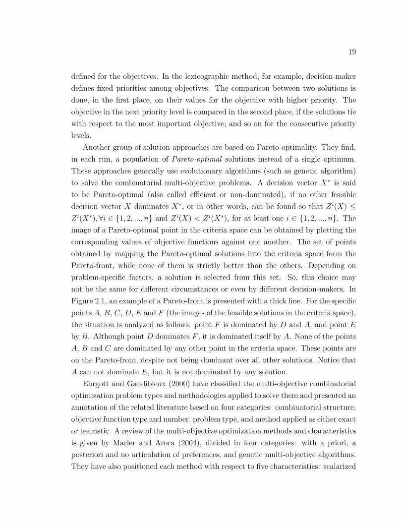
Ehrgott and Gandibleux (2000) have classified the multi-objective combinatorial

optimization problem types and methodologies applied to solve them and presented an

annotation of the related literature based on four categories: combinatorial structure,

objective function type and number, problem type, and method applied as either exact

or heuristic. A review of the multi-objective optimization methods and characteristics

is given by Marler and Arora (2004), divided in four categories: with a priori, a

posteriori and no articulation of preferences, and genetic multi-objective algorithms.

They have also positioned each method with respect to five characteristics: scalarized

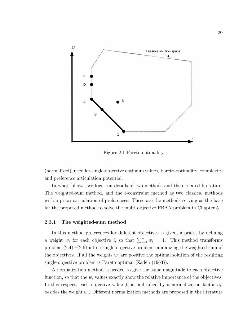
20

Z1

Z2

E

C

B

A

D

Feasible solution space

F

Figure 2.1 Pareto-optimality

(normalized), need for single-objective optimum values, Pareto-optimality, complexity

and preference articulation potential.

In what follows, we focus on details of two methods and their related literature.

The weighted-sum method, and the ε-constraint method as two classical methods

with a priori articulation of preferences. These are the methods serving as the base

for the proposed method to solve the multi-objective PBAA problem in Chapter 5.

2.3.1 The weighted-sum method

In this method preferences for different objectives is given, a priori, by defining

a weight wi for each objective i, so that∑n

i=1wi = 1. This method transforms

problem (2.4) –(2.6) into a single-objective problem minimizing the weighted sum of

the objectives. If all the weights wi are positive the optimal solution of the resulting

single-objective problem is Pareto-optimal (Zadeh (1963)).

A normalization method is needed to give the same magnitude to each objective

function, so that the wi values exactly show the relative importance of the objectives.

In this respect, each objective value fi is multiplied by a normalization factor ni,

besides the weight wi. Different normalization methods are proposed in the literature

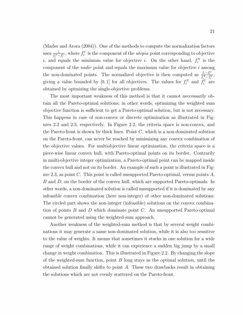
21

(Marler and Arora (2004)). One of the methods to compute the normalization factors

uses 1fNi −fUi

, where fUi is the component of the utopia point corresponding to objective

i, and equals the minimum value for objective i. On the other hand, fNi is the

component of the nadir point and equals the maximum value for objective i among

the non-dominated points. The normalized objective is then computed asfi−fUifNi −fUi

,

giving a value bounded by [0, 1] for all objectives. The values for fNi and fUi are

obtained by optmizing the single-objective problems.

The most important weakness of this method is that it cannot neccessarily ob-

tain all the Pareto-optimal solutions; in other words, optimizing the weighted sum

objective function is sufficient to get a Pareto-optimal solution, but is not necessary.

This happens in case of non-convex or discrete optimization as illustrated in Fig-

ures 2.2 and 2.3, respectively. In Figure 2.2, the criteria space is non-convex, and

the Pareto-front is shown by thick lines. Point C, which is a non-dominated solution

on the Pareto-front, can never be reached by minimizing any convex combination of

the objective values. For multiobjective linear optimization, the criteria space is a

piece-wise linear convex hull, with Pareto-optimal points on its border. Contrarily

in multi-objective integer optimization, a Pareto-optimal point can be mapped inside

the convex hull and not on its border. An example of such a point is illustrated in Fig-

ure 2.3, as point C. This point is called unsupported Pareto-optimal, versus points A,

B and D, on the border of the convex hull, which are supported Pareto-optimals. In

other words, a non-dominated solution is called unsupported if it is dominated by any

infeasible convex combination (here non-integer) of other non-dominated solutions.

The circled part shows the non-integer (infeasible) solutions on the convex combina-

tion of points B and D which dominate point C. An unsupported Pareto-optimal

cannot be generated using the weighted-sum approach.

Another weakness of the weighted-sum method is that by several weight combi-

nations it may generate a same non-dominated solution, while it is also too sensitive

to the value of weights. It means that sometimes it stucks in one solution for a wide

range of weight combinations, while it can experience a sudden big jump by a small

change in weight combination. This is illustrated in Figure 2.2. By changing the slope

of the weighted-sum function, point B long stays as the optimal solution, until the

obtained solution finally shifts to point A. These two drawbacks result in obtaining

the solutions which are not evenly scattered on the Pareto-front.

22

Z1

Z2

B

A

criteria space

w1

iZ1+w2

iZ2

C

Figure 2.2 Weighted-sum method with non-convex criteria space

Z1

Z2

D

Mapped feasible LP solution space

z=w1Z1+w

2Z2

Non-dominated integer solution

A

Dominating non-integer solutions

CB

Figure 2.3 Weighted-sum method for integer programming

23

2.3.2 The ε-constraint method

The ε-constraint method, proposed by Chankong and Haimes (1983) for multi-

objective optimization, is capable of finding also the unsupported Pareto-optimal

solutions. This method optimizes one of the objectives while putting bounds on

values of other objectives by adding a constraint for each of them. By varying the

value of bounds Pareto-optimal solutions are obtained. It may be also needed to solve

this problem for varying l values, specifying the minimization of different objectives

subject to the other values being bounded. While the feasible solution space and the

bound on value of i-th objective are denoted respectively by S and εi, the method is

formulated as follows:

minX

Z l(X) (2.7)

s.t.: Zi(X) ≤ εi, i ∈ 1, ..., n \ l (2.8)

X ∈ S. (2.9)

Using formulation (2.7)–(2.9), if we select the value of parameter ε equal to the value

of one of the objectives for point C in Figure 2.2, while minimizing the other objective,

we can obtain this point as the optimum solution. In case of integer optimization,

the added constraints have the role of cuts and introduce new extreme points. So

more branches are generated which result in higher computational time compared to

the weighted-sum method.

In order to improve the computational time incurred by the ε-constraint method

and also to introduce more applicability to this method, Ehrgott and Ryan (2002)

proposed a change to the formulation (2.7)–(2.9) for a bi-objective problem, which

permits small violation of the bound ε, in hopes of improving the other objective.

This is useful in practice when the first objective is the most important one. The

amount of violation is given by a surplus variable su, with a unitary penalty cost

of cpenalty. This penalty cost serves as the trade-off measure between the objective

functions. The new method is called the elastic-constraint method, as formulated in

the following:

minX

Z1(X) + cpenaltysu (2.10)

24

s.t.: Z2(X)− su ≤ ε, (2.11)

X ∈ S. (2.12)

All the Pareto-optimal solutions can be found by this method by varying the values

of ε and cpenalty. The ε-constraint and the weighted-sum methods are special cases of

the elastic-constraint method, resulted by special values for these two parameters.

The hierarchical method is a special case of the ε-constraint method. First, the

optimum value for the most important objective is found, then among the solutions

with value of the upper-level objective within a specified range of the optimum value,

the ones which optimize the objective in the next priority level are selected. This

procedure is continued to optimize all objectives in successive priority levels. The

drawback of this method is the increased probability of getting into infeasibilty in

the lower-level problems, due to the increased number of imposed constraints. The

lexicographic method (or multi-level programming) is a special case of the hierarchical

method with ε = Z2min(X), where Z2

min(X) shows the optimum value for the most

important objective.

The problem studied in Chapter 5 has two objectives one of which is hierarchically

more important, but its priority can be neglected to some extent in exchange for a

meaningful improvement in the other objective. That is why we propose to solve this

problem by implementing the elastic-constraint method with a hierarchical point of

view, by varying the value of ε close to the optimal solution for the first objective.

2.4 EMPLOYEE PREFERENCE SATISFACTION

Researchers have mostly studied employee preference satisfaction issues in airline

crew scheduling, rail crew scheduling, operating room scheduling, nurse rostering

and timetabling problems. Some of these works are summarized in the following

paragraphs.

2.4.1 Timetabling and activity assignment to work shifts

In Demassey et al. (2005) a constraint programming based CG method is used

for employee timetabling. This approach is also adapted to incorporate employee

preferences in assigning activities to personalized work shifts. This is done by associ-

ating to each employee, a different cost for the same assignment, according to his/her

25

preferences. These costs are put together with the coverage costs in a single objec-

tive function. Because of the decomposition method used, processing the constraints

and the global optimization is handled separately. The advantage of constraint pro-

gramming is its ability to model complex constraints and to handle variations of the

problem without major modifications to the algorithm.

2.4.2 Airline and rail crew scheduling

Airline crew scheduling may be performed in two planning levels. In crew pairing,

anonymous pairings/rotations are constructed such that the flights demand for crew

members is covered. A pairing is a sequence of different activities such as flight

legs, breaks and nighttime rests, starting and ending at the same crew base. In

another level, crew members are assigned blocks consisting of work (pairings) and

day-off schedules, called rosters during a month. This scheduling level is called crew

rostering. In practice we may consider crew preferences in constructing personalized

rosters. If the constructed rosters do not comply with crew preferences, or in other

words are anonymous, crew members bid for them afterwards. This process is called

bidline scheduling. In both cases, crew may be prioritized in getting satisfied with their

assigned schedules according to their seniority. If no seniority is considered among

crew members, assignment is said to be based on fair-share or equity. In preferential

bidding system (PBS), rosters are constructed while individual crew preferences are

treated in order of seniority. In what follows the related literature is reviewed.

Gamache et al. (1998) used the preferential bidding to solve the crew assignment

problem. This method constructs the personalized schedules for employees as in the

rostering problem but considering the employee preferences given as weighted bids.

Employees are sorted decreasingly based on their seniority, and starting from the

most senior one, for each employee a problem is solved by column generation which

assigns the schedule with the maximum total score to him while considering the

feasibility of assignment to the remaining employees based on the unassigned pairings.

Achour et al. (2007) proposed an exact CG approach for the PBS problem in which

employees bid for their preferred activities. The schedules are built sequentially in

order of employee seniority, covering all the pairings and assigning a schedule for each

employee. For the employee under consideration, it determines the best maximum-

score schedule given the fixed schedule scores for all employees already treated in the

previous steps. A schedule for the more senior employee is fixed only after it is proved

26

to be the only best schedule which yields the optimal score for the junior employees.

This is done by enumerating all the best-score schedules for each employee and then

by the help of some techniques reducing the set to include a single schedule.

A bi-criterion approach is applied by Moudani et al. (2001) for the medium-sized

nominal crew rostering problem which assigns the crew staff to pairings. Firstly, by a

heuristic procedure a set of solutions with maximized weighted crew staff satisfaction

on pairing preferences are found. Qualitative scales are used to characterize the

satisfaction degrees for crew staff, and each solution is obtained by a constructive

method which assigns the pairings to the sorted staff based on level of satisfaction,

starting by the staff with lowest satisfaction levels. Then a genetic algorithm is used

to generate new solutions with reduced operations costs.

Hansen and Liden (2005) established a constraint programming model which as-

signs airline crew members to groups such that the exceptions are minimized when

assigning schedules to the groups. An exception happens when it is not possible to

assign the same schedule to every crew in the same group. The crew in a same group

are matched based on the same or overlapping preferred days off, pre-assignments

like training courses, the preference to fly together, etc. The number and cost of

constructed groups is minimized, while groups are constructed as columns using a

branch-and-price algorithm.

In Dornberger et al. (2008) preference satisfaction corresponds to both company

and personnel in a multi-objective train staff planning problem. A railway company

may have preferences for assigning drivers to specific trains, due to their qualifications,

or for not assigning regular shifts to external drivers, due to the higher personnel costs.

On the other hand, train drivers in a senior group can demand for more attractive

work shifts to be assigned to. They are also assigned regular rosters, while the ones

in a junior group do not get any and should be on call too. Some other preferences

correspond to the distance of the starting or ending location to their residence or

on how the work ends prior to a vacation or start after a vacation. Considering

preferences also has the advantage of reducing the search space, from optimization

process point of view. First, a single-objective problem is proposed which sums up

the penalties for any shift violating preferences and constraints, with value of the

penalty depending on the type of violation. This summation is multiplied by a factor

standing for excess usage of resources. In another attempt, these three objective

are formulated separately forming a multi-objective optimization probelm, solved by

27

a genetic algorithm with a posteriori articulation of preferences to reflect the true

wishes of the decision-maker in the final selected decision.

Hanne et al. (2009) developed a decision support tool for rail crew rostering.

Preferences are defined for the company (based on favorability of assignments due to

qualification and experience of employees, and to reduce the personnel costs for certain

assignments), and the employees (for late or early shifts, or the gap between start/end

of tasks after/before the vacation). Three objective functions are introduced: the cost

function reflects the total costs of assignments for the company (based on duration

of shifts and cost per hour of each assignment); an objective function for minimizing

the deviations of service starting times from the employees preferred times; and the

last one maximizes the summation of the smallest gaps between either start or end

of vacation intervals and the assigned services for all the employees. There are also

some hard constraints for nonavailability times for drivers, non-overlaping and rest

times between services assigned to the same driver and qualification requirements.

Pareto-optimal solutions are obtained using an evolutionary algorithm.

Boubaker et al. (2010) developed an approximate set partitioning type model for

bidline scheduling with equity on number of days and paid hours for bidlines. The

proposed branch-and-price heuristic combined with a dynamic constraint aggregation

method results in better solutions in much less computational times for large instances

compared to the standard branch-and-price heuristic with rounding procedure.

In a crew rostering problem studied by Maenhout and Vanhoucke (2010), satisfy-

ing the preferences of crew members for the assigned activities and rest/work periods

is expressed as an objective of minimizing the penalty costs of assigning rosters to

the crew. This penalty is defined as the summation of the inverse of crew preferences

scores on the rosters attributes. Minimizing this penalty cost added to two other

cost objective values forms the objective function of the proposed model. These costs

include the penalty costs for deviating from the standard constraint values to pro-

vide fairness among the crew members; and the wage, undercovering and overcovering

costs. A hybrid scatter search method (a population-based metaheuristic) is proposed

to solve this problem, which relies on a column generation model. Subproblems are

resource constrained shortest path problems for each crew member.

28

2.4.3 Nurse rostering/operation room scheduling

Hospitals face varying nonstop patient demands, so the need for flexible nurse

schedules is more important in this service industry. With increasing shortage of

nurses, their preferences must be more considered in the scheduling process.

Ozkarahan (2000) proposed an enhanced version of the operating room scheduling

problem presented earlier as a goal programming model, which adds new goals for

respecting the preferences of surgeons for certain rooms and the importance of sched-

uled dates for some operations to the initial goals of rooms idle time and overtime

minimization. Knowing the patients scheduled for each surgeon and each day, this

model assigns each patient to a specific operating room and a starting time. As a

branch of multi-objective optimization, goal programming uses linear programming

to deal with multiple conflicting objectives or goals with target values to be achieved.

Ozkarahan’s model minimizes the weighted sum of deviations from targets with dif-

ferent priority levels. The weakness of this method is in setting the appropriate

weights.

Bard and Purnomo (2005) applied a heuristic CG method for a multi-objective

nurse scheduling problem, taking into account nurse preferences in taking days-off.

Penalties are considered in the objective function for the preference violations in the

constructed rosters, besides the personnel costs of adding outside nurses in case of

coverage shortage or undercovering cost. Providing balance in the satisfaction levels

for different nurses is also a measure of success. Thus, violation penalty cost of a given

schedule for a specific nurse is defined as an increasing function of the equivalent point

associated with the severity of the incurred violations. Columns are generated during

a procedure which identifies periods with under-coverage and over-coverage, and then

swaps the assignment of the corresponding nurse between two such periods to produce

a new candidate schedule. It is then verified if the new schedule is legal.

29

CHAPTER 3

A ROLLING HORIZON BRANCH-AND-PRICE HEURISTIC FOR

ACTIVITY ASSIGNMENT CONSIDERING FLEXIBLE FULL-TIME

SHIFTS

3.1 ACTIVITY ASSIGNMENT PROBLEM WITH FLEXIBLE REGU-

LAR FULL-TIME SHIFTS (AAFF)

The AAFF aims at determining a final working schedule of regular employees to

cover the demands of activities over a given horizon (typically, one day or one week)

that is partitioned into periods of equal length. In general, this problem is solved the

day or a few days before the operations when the demand forecasts are quite accurate.

At that moment, the work and rest days of each regular employee are already fixed

and planned shifts for their working days have been constructed. We call these shifts

the primary regular shifts and, for each of them, the following information is known:

the employee assigned to it, a pair of planned start and finish times, and a pair of

planned start and end times for a meal break (recall that we consider only full-time

shifts). Each primary regular shift is, thus, separated in two parts, called segments,

by its break. These primary regular shifts serve as inputs to the AAFF.

The inputs to the AAFF also include a set of activities. For each activity, the ideal

number of skilled employees required at each period of the horizon is given as well

as a minimum and a maximum number of consecutive periods for which an employee

can be assigned to this activity. All employees possess skills and can only be assigned

to activities for which they are skilled. In a period, an employee can only be assigned

to one activity, that is, partial activity covering is not allowed.

The activities must be assigned to the primary regular shifts which are, typically,

insufficient to offer a complete activity coverage. To increase coverage, the following

options are available. First, the primary regular shifts can be extended from one

end, which means, for example, that an eight-hour shift planned to start at 8:00 am

and end at 4:00 pm can be extended to start at 7:00 am or end at 5:00 pm. Such

an extension is subject to a maximum duration. Note that the one-end extension

restriction, which is imposed to offer more stability to the regular employees work

30

shifts, can easily be omitted in our solution approach. Second, the planned meal

breaks in the primary regular shifts can be moved. In this case, each shift segment

(including a possible extension) must respect a minimum and a maximum duration.

Given the available personnel, it often happens in practice that not all activity

demands are satisfied. Any undercovering yields a cost representing the loss of service

quality. In this chapter we consider that overcovering also yields a cost. Finally,

to reduce the loss of productivity occurring when an employee is assigned to two

different activities in two consecutive periods (that is, when an employee performs a

transition), transition costs are also taken into account.

The objective of the AAFF is thus three-fold. It consists of minimizing the total

of the activity undercovering costs, overcovering costs and the transition costs. In

general, the transition costs are of second order compared to the other costs, while the

undercovering costs are the most important ones. A solution to the AAFF indicates:

for each primary regular shift, its definitive start and end times and the position of

its meal break; and the activity assigned in each working period. Note that idling is

not allowed, as activity demand overcoverage (employee assignment excess to activity

demand in each period) is preferred to increase the quality of service.

The AAFF is defined as follows:

Inputs:

– The set of periods of time in the planning horizon.

– The set of activities.

– For each activity and each time period, a required number of employees.

– For each activity, a minimum and a maximum activity block duration.

– The set of available employees.

– Skills of each employee (i.e., the subset of activities to which they can be as-

signed).

– Start and end times of primary shifts.

– Length of the break for each work shift.

– Minimum and maximum duration of a segment.

– A maximum shift’s extension duration, knowing that extension is permitted

just at one end of a shift.

Decisions to take:

– Determining the shifts’ new start and end times, as well as new break place-

31

ments.

– Determining how to fill all the periods of the resulting segments with activities

for each employee.

Objectives:

To minimize the sum of the following:

– The cost of undercoverings for activities.

– The cost of overcoverings for activities.

– The cost of transitions.

Constraints:

– Each segment must be filled with activities.

– An employee can only be assigned to an activity if he is skilled for it.

– The minimum and maximum duration for an activity block must be respected.

– The number of employees assigned to each activity in each period must be equal

to the required number (soft constraint).

– A shift can be extended just from one end, and up to a maximum extension

duration.

– The minimum and maximum duration of a segment must be respected.

3.2 A ROLLING HORIZON BRANCH-AND-PRICE HEURISTIC

The AAFF problem can be modeled using variables showing the assignment of

each activity at each period to any shift. However, given the restrictions on the ac-

tivity assignment duration, such a model would be very large in practice and, thus,

difficult to solve. Here, we propose to formulate the problem as a generalized set

covering model with side constraints. Such a model was used by Dantzig (1954) for

a shift scheduling problem with break positioning decisions and a single activity and,

more recently, by Lequy et al. (2012a) for an activity assignment problem. For our

problem, it would require the enumeration of a very large number of shift activity

assignment patterns. To avoid enumerating all of them, a (heuristic) column gener-

ation method can be used. To further speed up the solution process, Lequy et al.

(2012a) suggest embedding this method into a rolling horizon procedure. Below, we

present the mathematical formulation, the rolling horizon procedure and the column

generation heuristic for AAFF problem.

32

3.2.1 Column Generation Formulation for AAFF

The model proposed for AAFF is the generalization of the CG formulation given

by Lequy et al. (2012a) which has permitted to obtain good results. In AAFF, the

meal break of every primary regular shift can be moved. Thus, for each such shift (and

its two segments), a set of feasible break start periods can be defined according to the

minimum and maximum duration of a segment and the possibility to extend one of its

segments. This is further explained in Section 3.3. For the presentation of the model,

we assume that for each segment of a primary regular shift and each corresponding

feasible break start period, one can enumerate all feasible segments that can replace

the primary segment, including a possible extension and the assigned activities. These

enumerated entities are referred to as Segment Extension/Activity (SEA) assignments.

Knowing to whom each of these SEA assignments are attributed, we are looking for

a combination of them for all the employees during the whole planning horizon that

minimizes the total costs. In this model, columns correspond to SEA assignments for

each pair of primary segment and possible break start.

To extend the model proposed by Lequy et al. (2012a), the following issues are

taken into account:

– The consecutivity of the first segment, the break, and the second segment of

each shift must be respected.

– The extension of each work shift from both ends is not permitted. This con-

straint is violated when our model chooses the first and second segments of a

given primary shift to have, respectively, an earlier start time and a later end

time than the current shift.

– The duration of each segment must fall within a given interval. The maxi-

mum duration is chosen so that a single break requirement for a shift would be

maintained.

– The maximum permitted shift extension must be respected.

The proposed master problem formulation relies on the following notation.

SetsP : Set of periods in the planning horizon (numbered from 1 to |P |).

A: Set of activities.

Pa: Subset of periods p ∈ P for which there is a demand for activity a ∈ A.

S1, S2: Set of the first (resp. second) segments of the primary regular shifts.

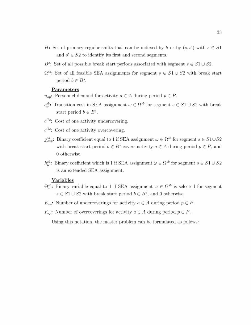
33

H: Set of primary regular shifts that can be indexed by h or by (s, s′) with s ∈ S1

and s′ ∈ S2 to identify its first and second segments.

Bs: Set of all possible break start periods associated with segment s ∈ S1 ∪ S2.

Ωsb: Set of all feasible SEA assignments for segment s ∈ S1 ∪ S2 with break start

period b ∈ Bs.

Parameters

nap: Personnel demand for activity a ∈ A during period p ∈ P .

csbω : Transition cost in SEA assignment ω ∈ Ωsb for segment s ∈ S1 ∪ S2 with break

start period b ∈ Bs.

cUc: Cost of one activity undercovering.

cOc: Cost of one activity overcovering.

gsbωap: Binary coefficient equal to 1 if SEA assignment ω ∈ Ωsb for segment s ∈ S1∪S2

with break start period b ∈ Bs covers activity a ∈ A during period p ∈ P , and

0 otherwise.

hsbω : Binary coefficient which is 1 if SEA assignment ω ∈ Ωsb for segment s ∈ S1 ∪ S2

is an extended SEA assignment.

Variables

Θsbω : Binary variable equal to 1 if SEA assignment ω ∈ Ωsb is selected for segment

s ∈ S1 ∪ S2 with break start period b ∈ Bs, and 0 otherwise.

Eap: Number of undercoverings for activity a ∈ A during period p ∈ P .

Fap: Number of overcoverings for activity a ∈ A during period p ∈ P .

Using this notation, the master problem can be formulated as follows:

34

min∑p∈P

∑a∈A

(cUcEap + cOcFap) +∑

s∈S1∪S2

∑b∈Bs

∑ω∈Ωsb

csbω Θsbω (3.1)

s.t.:∑s∈S1∪S2

∑b∈Bs

∑ω∈Ωsb

gsbωapΘsbω + Eap − Fap = nap, ∀a ∈ A, p ∈ P (3.2)∑

ω∈Ωsb

∑b∈Bs

Θsbω = 1, ∀s ∈ S1 ∪ S2 (3.3)∑

ω∈Ωsb

Θsbω −

∑ω∈Ωs′,b

Θs′,bω = 0, ∀(s, s′) ∈ H, b ∈ Bs (3.4)

∑ω∈Ωsb

∑b∈Bs

hsbω Θsbω +

∑ω∈Ωs′,b

∑b∈Bs′

hsbω Θs′bω ≤ 1, ∀(s, s′) ∈ H (3.5)

Θsbω ∈ 0, 1 , ∀s ∈ S1 ∪ S2, b ∈ Bs, ω ∈ Ωsb (3.6)

Eap, Fap ≥ 0, ∀a ∈ A, p ∈ P. (3.7)

Objective function (3.1) minimizes the total costs, including undercovering, over-

covering and transition costs. Constraint set (3.2) sets up the number of activity

undercoverings or overcoverings for each period, resulting from the selected SEA as-

signments. It is obvious that the variables Eap and Fap can not take both positive

values for each (a, p), since these variables appear with positive coefficients in the ob-

jective function to be minimized. So the absolute value of their difference represents

either the amount of overcoverage or undercoverage of each activity in each period.

Constraints (3.3) ensure that a SEA assignment is assigned to each regular shift seg-

ment. Constraint set (3.4) ensures the consecutivity of the selected SEA assignment

for the first segment, the meal break, and the selected SEA assignment for the second

segment forming a regular work shift. Constraint set (3.5) forbids the extension of

work shifts from both ends. Constraint sets (3.6) and (3.7) represent the domains of

the variables. Note that constraints (3.2) and (3.6), together with (3.1), guarantee

the integrality of the Eap and Fap variables. Finally, as in Lequy et al. (2012a), we

replace constraint set (3.2) by an equivalent form that reduces the constraint matrix

density and speeds up the solution process. This new form, formulated in constraint

set (3.8), is obtained by subtracting any two consecutive constraint in set (3.2) sorted

beforehand by activity types and then by ascending order of time periods. While

35

an activity block corresponds to the assignment of an employee to the same activity

for a number of consecutive periods, the resulted constraint matrix holds non-zero

values as SEA assignment’s coefficients only for the begin and the end periods of each

activity block.∑s∈S1∪S2

∑b∈Bs

∑ω∈Ωs

b

(gsbωap − gsbωa(p−1))Θsbω + Eap − Ea(p−1)

−Fap + Fa(p−1) = nap − na(p−1), ∀a ∈ A, ∀p ∈ P . (3.8)

3.2.2 Rolling Horizon Procedure

To obtain fast computational times, AAFF is solved using a rolling horizon proce-

dure which divides the horizon into overlapping time slices. Rolling horizon method

is categorized as constructive algorithms, which build the solution step by step by

assigning values to the variables. Like the other heuristic methods, the global opti-

mum is not guaranteed here. Contrarily, Local Improvement or Neighborhood Search

(NS) methods start with a feasible solution, and evaluate the feasible solutions in the

neighborhood of the current solution. The new solution will be the one that improves

the current solution to the greatest extent. This continues until no improvement can

be made to the current solution.

A Rolling Horizon heuristic is applied on medium to large-sized instances, in

order to get a reasonable computational time. Starting from the earliest time slice,

the procedure solves in chronological order a sequence of restricted problems, one

for each time slice. The solution of the problem associated with a time slice spans

this time slice and may even exceed it as discussed later. Except for the last time

slice, this solution defines initial conditions for the next time slice problem, as the

decisions made before this time slice are fixed while those in the overlap between

these two slices are reconsidered. These initial conditions are imposed by fixing the

SEA assignments at the beginning of the segments, yielding smaller set Ωsb for these

segments.

For a given time slice, the problem considered involves only the regular shifts

intersecting with this time slice. For the regular shifts, there are three kinds of

intersection with the time slice defined as follows.

Intersection kind 1: The shift begins within the time slice. In this case, no activity

assignment is fixed for this shift.

36

Intersection kind 2: The time slice begins within the first segment of the shift.

In this case, all activity blocks in the first segment (assigned in the previous

time slice solution) and ending prior to the start of the time slice are fixed.

Furthermore, the meal break and the shift start time are fixed.

Intersection kind 3: The time slice begins between the start of the meal break and

the end of the second segment of the shift. In this case, all activity blocks in

the first and second segments (assigned in the previous time slice solution) and

ending prior to the start of the time slice are fixed. Furthermore, the meal break

and the shift start time are fixed.

A schematic description of this rolling horizon procedure is given in Figure 3.1 for

a small instance. The horizontal and vertical axes show the time and the work shifts,

respectively. Part (a) illustrates the shifts in their primary status (primary start time,

end time and break position), numbered from 1 to 4 within diamonds, and with no

activities assigned yet. The black rectangles indicate meal breaks, whereas the hashed

rectangles show the parts of the segments to which activities must be assigned. To

start, based on the range of the first time slice specified in the figure, all the shifts

have intersection kind 1, shown within circles. In part (b), the solution of the first

time slice problem is presented, where the letters A, B and C denote the assigned

activity blocks. The primary start and end times of the shifts are labeled with st

and et to clearly identify which segments are extended. Part (c) shows the shifts to

consider in the time slice 2 problem. Based on the range of this time slice, shifts 1,

2 and 4 have intersection kinds 3, 1 and 2, respectively. Shift 3 has no intersection

and is thus considered final. For shift 1 with intersection kind 3, its start time and

its break position obtained in part (b) are fixed. The activity block intersecting with

the time slice 2 is removed, leaving a free space to be scheduled in this step. For its

second segment, only SEA assignments starting with the retained activity block B

are feasible. For shift 2 with intersection kind 1, any activity assigned previously is

removed and the shift start time, end time and break position are to be rescheduled.

For shift 4 with intersection kind 2, the start time and break position are fixed, the

end time is reset, and the intersecting assigned activity blocks are removed. At last

in part (d), the final schedule for the problem is illustrated. Note that, this method

causes the decisions concerning the flexible aspects of a shift being mostly made in the

first time slice intersecting with the shift. This can reduce the number of sub-problems

to be solved and, as a result, the computational time.

37

Time

shifts

Slice 1

Slice 1

et

st

B B A C B A B

CBABBB

Slice 2

(a)

(b)

(c)

(d)

st st

st

et

et et

et

st

B B

BBB

Slice 2

et

st

B B

BBB

C

et

A B

C B

et

et

st st

st

et

st

C

A B

11

11

13

2

1

3

2

4

Overlap

Figure 3.1 The rolling horizon procedure

Model (3.1), (3.3)–(3.8) needs adaptations for the problem restricted to a given

time slice. It must consider only the variables associated with the segments intersect-

ing with the time slice. These variables are further restricted to the admissible SEA

assignments according to the shift intersection kind (that may fix the meal break

position and some activity blocks). Only the constraints corresponding to these

segments are considered in constraint sets (3.3)–(3.5). As for the activity demand

constraints (3.8), they are restricted to the periods between the first and the last

period in which at least one activity assignment decision must be made in this time

slice. The right-hand side of the constraints associated with a period before the start

of the time slice are updated according to the fixed activity assignments (from the

previous time slice). Finally, constraint sets (3.4) and (3.5) consider only the shifts

with intersection kind 1. In case of intersection kind 2 and 3, these constraints become

redundant. On the one hand, only the fixed meal break is considered for generating

the admissible SEA assignments, and on the other hand, the fixed start time for shifts

with intersection kinds 2 and 3 restricts the shift extension possibilities in admissible

SEA assignments generated for the corresponding segments. This concept is further

detailed in Section 3.2.3

38

3.2.3 Column generation heuristic

To obtain relatively fast computational times, the time slices of the rolling horizon

procedure should be relatively short. On the other hand, they should not be too

short to ensure a more global view of the solution process in each time slice. In

this case, model (3.1), (3.3)–(3.8), adapted to the current time slice, contains a very

large number of decision variables. Column Generation (CG) (Barnhart et al. (1998);

Lubbecke and Desrosiers (2005); Desaulniers et al. (2005)) is an efficient method for

solving the problems with a large number of variables. This method can only solve

linear relaxations and must, therefore, be embedded into a MIP procedure to find

integer solutions. Here we use a branch-and-bound (B&B) heuristic to find integer

solutions. When column generation is embedded into a B&B method, it is known as

branch-and-price (B&P) method (Desaulniers et al. (2005); Barnhart et al. (1998)).

In the context of a column generation method, the linear relaxation to solve is

called the master problem. Starting with an initial solution to the master problem,

this iterative method solves at each iteration the master problem restricted to a

subset of its variables, called the restricted master problem (RMP), and one or several

subproblems that generate new variables (columns) to add to the RMP. Given a

dual solution to the current RMP, the subproblems search for negative reduced cost

columns. If no such columns exist, then the column generation process stops as

the current primal RMP optimal solution is also optimal for the master problem.

Hence, with this solution method, we avoid dealing with all the variables by rather

adding them gradually into the model until no improvement can be gained in the

objective function value. Generated columns and coefficients are inserted into the

RMP formulation to be solved.

The master problem for AAFF corresponds to the linear relaxation of model (3.1),

(3.3)–(3.8), adapted to the current time slice. To start the column generation process,

we need to have a feasible initial solution for the master problem. This solution is

obtained by adding dummy variables to the constraint set (3.3). To avoid having

these dummy variables in the final solution, large costs are defined for them. The

dual variables of the master problem are denoted as follows:

πap, ∀a ∈ A, p ∈ P , for constraints (3.8);

τs, ∀s ∈ S1 ∪ S2, for constraints (3.3);

λbs,s′ , ∀(s, s′) ∈ H, b ∈ Bs, for constraints (3.4); and

39

νs,s′ , ∀(s, s′) ∈ H, for constraints (3.5).

Every RMP involves all the Eap and Fap variables. Therefore, only the Θsbω variables

are generated by the subproblems. There is a subproblem for every pair of regular shift

first segment and break start period, and every pair of regular shift second segment

and break start period involved in the current time slice. Let S1In and S2In be the

subsets of these entities, respectively. Denote by BsIn and Ωsb

In the subsets of break

start periods and SEA assignments valid for segment s ∈ S1In ∪ S2In according to

the intersection kind of the shift containing s and break start period b. Let s ∈ S1In

be the first segment of a regular shift h ∈ H, b ∈ BsIn a break start period for s and

ω ∈ ΩsbIn a SEA assignment for s. The reduced cost csbω of the corresponding variable

Θsbω is given by

csbω = csbω −∑a∈A

∑p∈P

(gsbωap − gsbωa(p−1))πap − τs − λbs,ρ2(s) − νs,ρ2(s)hsbω , (3.9)

where ρ2(s) indicates the second segment of shift h, that is, (s, ρ2(s)) ∈ H. The

subproblem for segment s and break start period b ∈ BsIn can be stated as

minω∈Ωsb

In

csbω ,

where its constraints are implicitly given by definition of the set ΩsbIn. As described

below, these constraints can correspond to those of a shortest path problem.

Similarly, for the second segment s ∈ S2In of a regular shift h ∈ H and a break

start period b ∈ BsIn, the reduced cost csbω of a variable Θsb

ω , ω ∈ ΩsbIn is

csbω = csbω −∑a∈A

∑p∈P

(gsbωap − gsbωa(p−1))πap − τs + λbρ1(s),s − νρ1(s),shsbω , (3.10)

where ρ1(s) indicates the first segment of shift h. Their corresponding subproblem is

minω∈Ωsb

In

csbω ,

where its constraints are also implicitly stated in the definition of set ΩsbIn.

Every subproblem can be modeled as a shortest path problem defined over an

acyclic network and solved using dynamic programming. For a subproblem associated

with segment s ∈ S1In∪S2In of a regular shift h ∈ H and a break start period b ∈ BsIn

40

such a network is described as follows. Denote by P sbIn the subset of periods that can

be covered by segment s (that is including the possible extension if any) considering

the break start period b, and by QsbIn the subset of periods at which segment s ∈ S1In

can start or segment s ∈ S2In can end. These two sets are known for each first or

second segment and each possible break start for the corresponding shift, based on

the formulations which will be given later in Section 3.3. Also denote by DsbIn the

set of activity blocks fixed from previous time slice for segment s ∈ S1In ∪ S2In and

break start period b ∈ BsIn. A fixed activity block d ∈ Dsb

In corresponds to activity

type ad starting at period pfd and ending at period ptd.

Such a network can contain up to four types of nodes, where Ah is the subset of

activities a ∈ A which can be assigned to primary regular shift h ∈ H (considering

employee skills): 1) a source node α, 2) a sink node β, 3) a start of activity block node

Bap for each period p ∈ P sbIn and each activity a ∈ Ah, and 4) an end of activity block

node Eap for each period p ∈ P sbIn and each activity a ∈ Ah. Figure 3.2 provides an

example of such a network for a first segment related to a shift with intersection kind 1,

without fixed activities from the previous time slice. The horizontal axis represents

the time and the activities are spread along the vertical axis. P sbIn comprises four

periods, numbered from 1 to 4, and QsbIn = 1, 2, 3. st = 3 indicates the start time

of the segment in the primary shift, b = 5 the start period of the meal break. In this

example, there are two activities, numbered 1 and 2, and an activity block must last

one or two periods for activity 1 and two or three periods for activity 2.

Such a network can contain up to five arc types.

1. Start of segment arcs.

2. End of segment arcs.

3. Activity block arcs.

4. Transition arcs.

5. Fixed activity block arcs.

The arcs on the networks related to a segment s ∈ S1In ∪ S2In of a regular shift

h ∈ H and a break start period b ∈ BsIn, and the costs associated with them are

described in Table 3.1. Denote by q, the length of the break in number of periods,

by cTrs the cost of one transition, by ph1 and ph2 the periods immediately before the

start and immediately after the end of shift h ∈ H, respectively, and by dmina and

dmaxa the minimum and maximum duration of an assignment block for activity a ∈ A,

41

st

Activity 2

β

E23

E13

B13

B23

E22

E12

B12

B22

α

Activity 1 E11

B11

B21

b

E23

E13

B13

B23

E24

E14

B14

QIn

sb

PIn

sb

Figure 3.2 Example of a network for a first segment s ∈ S1In with possible extension

respectively.

In Figure 3.2, the start and end of segment arcs are represented with dashed

arrows, the activity block arcs with solid arrows, and the transition arcs with dotted

arrows. In such a network, a path from the source node to the sink node represents a

feasible SEA assignment for segment s and break start period b. The cost of this path

is equal to the reduced cost of the corresponding Θsbω variable. The network without

extension can easily be deduced from the one described above.

In practice, the number of subproblems can be relatively large and the number of

negative reduced cost columns found by these subproblems can be quite high for most

column generation iterations. In order to limit the number of columns generated at

each iteration, we develop the following strategy. In fact, because constraints (3.4)

and (3.5) impose, for each pair of segments (s, s′) ∈ H, the selection of two SEA

assignments (one for each segment) that share the same break start period and at most

one can be extended, we propose to avoid generating such assignments independently.

Two such assignments (or their corresponding columns) and the subproblems that can

generate them are said to be complementary. For each subproblem associated with

a first segment s ∈ S1In and a break start period b ∈ BsIn or with a second segment

s ∈ S2In and a break start period b ∈ BsIn, denote by CSP sb its complementary

subproblem.

42

Table 3.1 Definition of arcs in subproblem of segment s ∈ S1In ∪ S2In

Type Origin Destination Cost

1 α Ba,p,∀a ∈ Ah,if s ∈ S1In :∀p ∈ QsbIn,if s ∈ S2In :p = b+ q

if s ∈ S1In:

−τs − λbs,ρ2(s) if p = ph1 + 1

−νs,ρ2(s) otherwise,

if s ∈ S2In:− τs + λbρ1(s),s

2 Ea,p,∀a ∈ Ah,if s ∈ S1In :p = b,if s ∈ S2In :∀p ∈ QsbIn

β if s ∈ S1In: 0,

if s ∈ S2In:

0 if p = ph2 − 1

−νρ1(s),s otherwise

3 Ba,p,∀a ∈ Ah,∀p ∈ P sbIn

Ea,p+j−1,dmina ≤ j ≤ dmaxa ,p+ j − 1 ∈ P sbIn,[p, p+ j − 1] ∩[pfdsb, p

tdsb] = ∅,

∀d ∈ DsbIn

πa,p+j − πa,p

4 Ea,p,∀a ∈ Ah,if s ∈ S1In :∀p ∈ P sbIn\b−1,if s ∈ S2In :∀p ∈ P sbIn \ ph2

Ba′,p+1,∀a′ ∈ Ah\a cTrs

5 Badpfd,

∀d ∈ DsbIn

Eadptd , 0

At each column generation iteration, we use the procedure described in Algo-

rithm 1 to generate the columns, where HIn denotes the subset of regular shifts

intersecting with the current time slice. For a regular shift with intersection kind 1,

if the column with the least reduced cost for the first segment represents an extended

SEA assignment, then for the complementary subproblem of the second segment no

extension is allowed. Also, knowing to which break start the least reduced cost col-

umn corresponds, we only solve the subproblem corresponding to that break start for

the second segment. So a maximum of four columns can be generated, that is, the

column with the least reduced cost for each segment and a complementary column

for each of them. For a regular shift with intersection kind 2, a maximum of two

columns can be generated because the break start period b∗ is fixed. For a regular

shift with intersection kind 3, a single column can be generated for the second seg-

ment (the SEA assignment for the first segment being fixed, it can be added a priori

43

to the RMP). By using this strategy we make sure that firstly, at each iteration we

add the best column for each of the segments of a shift, and secondly, we save time

by generating only the columns with the required characters.

As mentioned above, column generation allows to solve the linear relaxation of

model (3.1), (3.3)–(3.8), adapted to the current time slice and, thus, provides a lower

bound on the optimal integer solution value. If the computed solution is integer, then

it is optimal. Otherwise, we use a rounding procedure using a branching tree with a

single branch, to get an integer solution. Given a fractional solution, this procedure

fixes to 1 all fractional-valued variables Θsbω that take a value greater than or equal

to a predefined threshold (0.75 for our tests). If no such variables exist, just one

fractional-valued variable whose value is the nearest to 1 is fixed at 1. Once these

decisions are imposed, the column generation process is started again to compute a

new linear relaxation solution and rounding is repeated if necessary. This iterative

process continues until obtaining an integer solution. Note that, after each rounding

step, the variables corresponding to the previously generated columns which are not

complementary to the newly fixed columns are removed from the RMP by fixing their

values to 0. Knowing to which shift and which segment any of the fixed variables

corresponds, we generate a complementary column for each of the fixed columns.

Once a column is fixed at 1 for the first or second segment of a regular shift with

intersection kind 1, then this fixes the break start period of the shift and determines

QsbIn for the other segment, then all subproblems associated with this shift except one

become useless.

Unhelpful extensions may happen in the final solution, because we relax flexibil-

ities in the passage from one time slice to the other, and so causing the algorithm

to lose the opportunity to correct the bad decisions it has made during the previous

steps. At the end of the rolling horizon algorithm, all the extensions made to the

shifts are reviewed. If during any interval including the furthest period of a shift

extension we are assigning the employee an activity which is overcovered during the

whole interval, the redundant extended part is removed, provided that the resulting

segment duration and activity duration remain above the minimum limits.

44

Algorithm 1 Solving the subproblems

1: for all regular shift h = (s, s′) ∈ HIn do2: nofirstsegment=false3: if h has intersection kind 1 then4: Solve all subproblems associated with segment s and a break start period

b ∈ BsIn

5: if the least reduced cost column found has a negative reduced cost then6: Add this column to RMP and denote by b∗1 the corresponding break start

period7: Solve subproblem CSP s,b∗1 for segment s′

8: if the least reduced cost column found has a negative reduced cost then9: Add this column to RMP10: else11: nofirstsegment=true12: Solve all subproblems associated with segment s′ and a break start period

b ∈ BsIn

13: if the least reduced cost column found has a negative reduced cost then14: Add this column to RMP and denote by b∗2 the corresponding break start

period15: if nofirstsegment=false then16: Solve subproblem CSP s′,b∗2 for segment s′

17: if the least reduced cost column found has a negative reduced cost then18: Add this column to RMP19: else if h has intersection kind 2 then20: Solve the subproblem for segment s with the fixed break start period b∗

21: if the least reduced cost column found has a negative reduced cost then22: Add this column to RMP23: Solve subproblem CSP s,b∗ for segment s′

24: if the least reduced cost column found has a negative reduced cost then25: Add this column to RMP26: else27: Solve subproblem CSP s,b∗ for segment s′

28: if the least reduced cost column found has a negative reduced cost then29: Add this column to RMP

45

3.3 DEFINING FLEXIBILITIES

For each segment s ∈ S1 ∪ S2 the following should be defined to construct the

subproblems:

– the set of feasible break start periods Bs,

– subsets of periods Qsb at which segment s ∈ S1 can start, or segment s ∈ S2

can end for each break start b ∈ Bs.

Feasible break starts for each shift should satisfy the requirements for segments du-

ration considering the possible extension to the shifts. We use the following notation

extmax: Maximum extension time for a flexible full-time shift (in periods),

kmin: Minimum duration of each segment s ∈ S1 ∪ S2 (in periods),

kmax: Maximum duration of each segment s ∈ S1 ∪ S2 (in periods),

bse: earliest possible break start period for segment s ∈ S1 ∪ S2,

bsl : latest possible break start period for segment s ∈ S1 ∪ S2,

psbes: earliest possible start period for segment s ∈ S1 with break start b ∈ Bs,

psbls : latest possible start period for segment s ∈ S1 with break start b ∈ Bs,

psbee: earliest possible end period for segment s ∈ S2 with break start b ∈ Bs,

psble : latest possible end period for segment s ∈ S2 with break start b ∈ Bs.

in the formulations to obtain these time periods, given as:

bse = max ph2 − 1− q − kmax , kmin + ph1 + 1− extmax , (3.11)

bsl = min ph1 + 1 + kmax , ph2 − 1 + extmax − kmin − q , (3.12)

psbes = max b− kmax , ph1 + 1− extmax , (3.13)

psbls = min b− kmin , ph1 + 1 , (3.14)

psbee = max b+ q + kmin , ph2 − 1 , (3.15)

psble = min b+ q + kmax , ph2 − 1 + extmax . (3.16)

Equation (3.11) is justified since the earliest break start can possibly happen when

the second segment takes its maximum possible length in the non-extended status.

However, this would not be a feasible start for break if the remaining length for the

46

first segment, even by extending it to maximum, is shorter than the minimum permit-

ted length. A mirrorwise logic applies to Equation (3.12). Based on Equation (3.13),

for a specific break start, the shift’s earliest start is when the maximum permitted

length is considered for the first segment, on condition that it is not earlier than the

start time resulting from the maximum permitted extension to the shift. On the

other hand, Equation (3.14) shows that the latest possible start for a specific break

start occurs when the first segment has the minimum permitted length, subject to

not starting later than the primary start. If the latest start obtained for the shift is

earlier than the shift’s primary start, we are not allowed to have an extension at the

end of the shift for that break start due to the constraint (3.5). Otherwise, Equations

(3.15) and (3.16) are applied to obtain the possible segment end time for a specific

break start, based on a similar mirrorwise logic.

Accordingly, the following ranges define the set of break start periods and the

possible start and end periods for a first or second segment for each break start

identified:

Bs = [bse, bsl ], ∀s ∈ S1 ∪ S2 (3.17)

Qsb = [psbes, psbls ], ∀s ∈ S1 (3.18)

Qsb = [psbee, psble ]. ∀s ∈ S2 (3.19)

Note that P sb for break start period b is the subset of periods that can be covered by

segment s including the possible extension. So P sb is the union of Qsb and primary

working periods of the segment considering break start period b. The subsets of

periods BsIn = Bs, Qsb

In = Qsb, and P sbIn = P sb are defined in the current time slice

of the rolling horizon, if there is an intersection kind 1 for the corresponding regular

shift. For intersection kinds 2 and 3, BsIn is confined to the fixed break start. For

intersection kind 2, QsbIn includes the fixed start time for a first segment s ∈ S1In.

To form a complementary subproblem in case of intersection kinds 2 and 3, QsbIn for

the second segment s ∈ S2In is equal to either Qsb, if the fixed start for the first

segment does not show an extension to the shift; or the primary end time of the

shift, otherwise. P sbIn is obtained in intersection kinds 2 and 3 for any of the segments,

knowing the set of periods QsbIn and the fixed break start period.

47

3.4 EXPERIMENTATION

We have tested the proposed rolling horizon heuristic on two classes of small-sized

instances and one class of medium-sized instances generated by Lequy et al. (2012a).

The work shifts in these instances are considered as ”primary regular shifts” for the

AAFF model. The AAFF model is more complex than the multi-activity assignment

problem (MAAP) proposed by Lequy et al. (2012a) due to the added flexibilities.

The purpose of these experiments is to study the effects of adding flexibility options

to shift schedules on activity assignment to work shifts. For our tests, we used the

Xpress-MP solver (version 7.2.1) of the Fair Isaac Corporation for solving all linear

and integer programs. All our experiments were conducted on an Intel R©Core TM2

CPU 6700 processor clocked at 2.66GHz with 4GB RAM.

3.4.1 Test Instances

The first class of small-sized instances includes regular shifts for 20 employees, to

be assigned activities among 5 types, over a one-week horizon. The second small-

sized class represents instances with 50 employees and 10 activities over one day. The

medium-sized class includes instances with 50 employees and 7 activities over one

week. Each class includes 5 randomly generated instances that replicate real-world

instances, which may be encountered in large retail stores or leisure resorts. In all

instances, the planning horizon is divided into 15-minute periods.

3.4.2 Test Assumptions

The followings are the parameters considered in our experiments:

extmax = 4, kmin = 16, kmax = 28, cOc = 150, cUc = 1500, cTrs = 15, and q = 30.

Values of dmina vary between 4 and 9 periods for different activities, and dmaxa = 14

periods for all activity types.

The following hypotheses are assumed as the basis for our experimental tests:

– AAFF considers only one break per shift. We consider this is a lunch break

with the same duration for all shifts. There may be some short breaks during

a shift in practice, which are not considered here.

– The purpose of this model is only to show the coverage improvements that can

be achieved by using flexibilities. It is assumed that each employee can start his

work a little earlier or end it a little later than what was preliminarily set for

48

him, with no cost, in order to improve the service level. It is the overcovering

cost that preclude unhelpful shift extensions.

3.4.3 Parameters Fitting

The quality of the solutions yielded by the rolling horizon algorithm depends on

the following parameters:

sl: The length of each time slice (in number of periods).

ov: The length of overlapping between time slices (in number of periods).

Depending on the values set for sl and ov, we get solutions with different qualities

and computational times for each instance. For each class, these values were chosen

based on preliminary test results for 5 instances. For each pair of parameters (sl, ov)

tested, the average of computational times of the 5 instances and also the average of

costs obtained are calculated. Finally sl and ov amounts are set to be equal to 60 and

20, respectively, for the second small-size class, and equal to 96 and 32, respectively,

for the first small-size class and the medium-size class of instances. The selected

pair of values was the one offering a good trade-off between solution quality and

computational time.

3.4.4 Computational Results

To assess the efficiency of the AAFF model in using flexibility options to improve

demand coverage, the results of the rolling horizon heuristic is compared to the best

solutions with no flexibility obtained in each class of instances by Lequy et al. (2012a).

The results on small-sized instances are compared to the exact solutions using the

”Block” model. This model gives a reformulation of the multi-commodity network

flow model with less number of constraints and only activity block arcs in the net-

works. Each block is associated with a single activity and represents the assignment

of the employee associated with a shift segment to that activity, for a consecutive

number of periods representing the activity assignment duration rules. With this

model, paths are not explicit, they need to be constructed afterwards from the values

of binary arc flow variables. Reformulated constraints only ensure coverage of every

period of each segment by an activity arc, and no occurence of consecutive activity

arc flows for a same activity type. For medium-sized instances our results are com-

pared to the ones using column generation based rolling horizon called ”Horizon CG”.

49

Lequy et al. (2012a) failed to find good-quality solutions in reasonable computational

times by exact methods, while showed the efficiency of ”Horizon CG” compared to

the block model rolling horizon heuristics for medium-sized instances. The results for

each class is separately presented in Tables 3.2, 3.3 and 3.4.

Table 3.2 Results for 7 days, 20 shifts per day, and 5 activities (class 1)

Ins. AAFF-Horizon CG MAAP-Exact B&B-Block Model

Cost #Uc T(s) #Ext %Ext %Ext.shifts

%Oc Cost #Uc T(s) %Oc

2732 28200 7 835 73 1.6 27 1.8 33600 17 21 0.41024 24705 5 899 78 1.7 39 1.8 45720 25 17 0.61773 30285 9 669 73 1.6 29 1.8 34065 18 17 0.45553 21975 3 861 78 1.7 33 1.8 41415 22 34 0.54657 31095 7 986 101 2.2 37 2.4 37200 20 135 0.4

Table 3.3 Results for 1 day, 50 shifts per day, and 10 activities (class 2)

Ins. AAFF-Horizon CG MAAP-Exact B&B-Block Model

Cost #Uc T(s) #Ext %Ext %Ext.shifts

%Oc Cost #Uc T(s) %Oc

5226 4545 0 7281 17 1 22 1 15045 8 93 0.55135 4575 0 1419 17 1 24 1 11820 6 98 0.31808 4710 0 13251 18 1 24 1 20190 11 1190 0.65066 5100 0 7918 19 1.1 18 1.1 5520 2 294 0.18854 5595 1 28376 11 0.6 18 0.7 10440 5 321 0.3

The first column shows the instance solved. The next seven columns give the

results for the heuristic column generation method proposed for the AAFF problem

as follows. ”Cost” represents the cost of the solution, ”#Uc” is the number of un-

dercoverings in periods, and ”T(s)” shows the solution time in seconds. ”#Ext” is

the number of extensions in periods. ”%Ext” shows the rate of shift extension time

to the regular working time. ”% Ext. shifts” shows what percentage of the total

number of shifts are extended. Finally, ”%Oc” gives the percentage of overcovered

demands. The last four columns of the tables show the information on the solutions

for the MAAP model given by Lequy et al. (2012a).

50

Table 3.4 Results for 7 days, 50 shifts per day, and 7 activities (class 3)

Ins. AAFF-Horizon CG MAAP-Horizon CGCost #Uc T(s) #Ext %Ext %Ext.

shifts%Oc Cost #Uc T(s) %Oc

237 41145 8 35580 105 0.9 20 1 41310 18 333 0.21007 35625 6 41254 90 0.8 18 0.9 46605 21 363 0.24369 28515 3 82368 75 0.7 14 0.7 41610 18 473 0.2156 36585 5 45150 102 0.9 16 1 25890 8 612 0.15216 25650 0 52480 87 0.8 17 0.8 50460 23 543 0.2

Comparing the number of undercoverings (the main part of the objective function)

in the solutions obtained for the AAFF problem by using the RH method, with those

of the MAAP with no flexibility shows that by including flexibility options the number

of undercoverings is reduced on average by 68%, 96%, and 70% in first, second and

third classes, respectively. These improvements are made by extending the regular

working time by 1.8%, 0.9% and 0.8% on average for class 1, 2 and 3 instances,

respectively. These extensions correspond to 33%, 21% and 17% of the total number

of shifts, respectively. Although, the computational times are much higher for AAFF,

it is shown in Chapter 4 that by removing the unhelpful options for shifts extensions

deliberately in advance it is possible to reduce the complexity of the AAFF problem,

in hopes of getting better computational times.

Note that all the above instances are generated so that the total demand for

all activities in each period is equal to the total number of available employees in

that period. So for any solution keeping the primary status of shifts, the number of

overcoverings and undercoverings in each period, and so their total numbers in that

solution, are always equal. Contrarily, this is not true for the solutions with shifts

extensions in the AAFF problem anymore. For example, extending a shift to a period

with undercoverings, may save an undercovering, but at the same time may bring

several overcoverings to the earlier periods in the shift extension. So the trade-off

between the number of saved undercoverings and increased overcoverings determines

the extensions to the work shifts. The average percentage of overcoverings in three

classes of instances are respectively equal to 1.9%, 1% and 0.9%, by considering

flexibility options. By considering flexibilities, the number of overcoverings resulted

for an instance is on average 4.3, 3.7, and 6.5 times more than the case with no

flexibility considerations, respectively in first, second and third classes.

51

3.5 CONCLUSION

The problem of assigning different activities to employees with predetermined work

shifts is by itself a complex problem. In this problem the purpose is generally to find

a combination of assignments which comply with the activities duration bounds and

employees qualifications while bearing the minimum costs. The most important part

of incurred costs in such a problem is related to the coverage of demands for activities.

Each activity requires a specific minimum number of employees to work on in each

period of time during the planning horizon. Any shortage of employees assigned to

any activity in any period lowers the customer service quality which consequently

imposes costs on the company. These costs are known as undercovering costs.

The problem we address in this chapter and the following one is even more com-

plex. Since better knowledge of demands is acquired just a few days before the

operations, we consider some scheduling flexibilities to help us cover the demands

better. In this chapter these flexibilities include meal break repositionings, and flexi-

ble start or end of the shifts, although breaks, start and end times were preliminarily

determined. For this problem, we developed a column generation formulation, and a

branch-and-price heuristic embedded into a rolling horizon procedure is used to solve

large-sized instances. The added flexibilities increase substantially the number of

columns and therefore the computational times to a great extent. The results of this

chapter show great savings in the number of activity demand undercoverings because

of the additional flexibilities, compared to the original problem without flexibilities.

The work done in this chapter serves as a preliminary step to introduce flexibilities

to work shifts, for further improving this application in the next chapter; since the

reported computational times in this chapter are not satisfactory.

52

CHAPTER 4

A TWO-LEVEL HEURISTIC METHOD FOR ACTIVITY/TASK

ASSIGNMENT CONSIDERING TEMPORARY AND FLEXIBLE

FULL-TIME SHIFTS

4.1 TASK SCHEDULING AND ACTIVITY ASSIGNMENT TO TEM-

PORARY AND FLEXIBLE REGULAR FULL-TIME SHIFTS (AT-

TFF)

In Chapter 3, the results showed that by extending the regular shifts or moving

their breaks better coverage can be obtained for activities, but with very high com-

putational times for the proposed RH heuristic. On one hand, the present chapter

aims at reducing the complexity of AAFF problem, in hopes of getting better compu-

tational times, by removing the unhelpful options for shifts extensions deliberately in

advance. On the other hand, it brings other flexibilities to the problem by introduc-

ing ATTFF problem. In ATTFF, there are some tasks to be scheduled in addition

to the activities. Each task must be accomplished once by a single skilled employee

over a consecutive set of periods. It is defined by a fixed duration and a time interval

during which it must start. In a period, an employee can only be assigned to one

task or one activity, so similar to activities partial task covering is not allowed. Em-

ployees can only be assigned to tasks for which they are skilled. In addition to the

working schedule flexibilities considered in AAFF, the ATTFF aims at scheduling for

temporary employees. Using temporaries gives more flexibility to scheduling and is

highly desirable for companies to overcome demand changes, since their shifts can

be inserted whenever needed. On the one hand, the proportion of time worked by

the temporary employees (and possibly the regular part-timers, if any) over the total

working time must respect an upper bound imposed by labor union rules. It is also

preferable for companies to limit this proportion, since adding the temporaries to the

staff requires extra training. On the other hand, the temporaries usually look for a

guaranteed minimum number of worked hours, otherwise they may find another job.

A lower bound may also be required in order to avoid excessive workload assigned to

regular workers. As it is typically the case in practice, we assume that the temporary

53

shifts are relatively short (say, between three and five hours), do not contain a meal

break and are scheduled during the day. We also assume that all the temporaries

possess the same skills which allow them to perform only a few basic activities with

high demands. They cannot be assigned to tasks which are dedicated to the regular

employees. The number of temporaries available each day is known. Additional costs

must also be paid for each period that a regular employee works in overtime, and also

for each period of a temporary shift. The objective of the ATTFF consists of mini-

mizing the costs for the temporaries and the overtime costs besides the undercovering

and transition costs. Notice that in ATTFF, the transitions also happen between two

different tasks or a task and an activity in two consecutive periods. In addition to the

outputs of AAFF, by ATTFF we schedule and assign the tasks, select the temporary

shifts and assign activities to each period of the temporary shifts.

4.2 A TWO-PHASE HEURISTIC FOR THE ATTFF

The ATTFF can be modeled as a mixed-integer program that, for real-life in-

stances, would not be solvable in reasonable computational times (see the model and

the computational results of Lequy et al. (2010), for a similar, but less complex activ-

ity/task assignment problem). Consequently, we propose to solve the problem in two

phases: the first phase handles task scheduling and task assignment, and determines

potential temporary shifts and potential regular shift extensions. Temporary shifts

and regular shift extensions without potential are left out of the second phase in order

to derive fast computational times. Then the second phase consists of assigning the

activities to the shifts taking into account the tasks already assigned as well as the

temporary shifts and the regular shift extensions identified in the first phase. Meal

breaks can also be moved.

4.2.1 First phase

In the first phase of the heuristic, we propose to use an approximate MIP model

of the ATTFF, which is a generalization of Jin (2009) model that includes variables

for regular shift extensions and temporary shifts. This model approximates the AT-

TFF for different reasons: integrality on certain activity assignment variables and

bounds on the activity assignment durations are relaxed; regular shift breaks cannot

be moved; tasks cannot be covered in shift extensions; and transition costs are not

54

considered. We assume that there is a limited number of potential temporary shifts

(defined by a start period and a shift length) that can be enumerated a priori. Copies

of the temporary shifts can be used to allow the assignment of several temporary

workers to the same shift.

The first phase model relies on the following notation, in addition to the ones

given in Chapter 3.

SetsPOih : Set of periods in the possible extension of the ith segment (i = 1, 2) of shift

h ∈ H.

PRh : Set of working periods p ∈ P in primary regular shift h ∈ H.

HAap: Subset of primary regular shifts h ∈ H which can be assigned activity a ∈ A at

period p ∈ P (considering shift start and end times, possible shift extensions,

shift meal break and employee skills).

L: Set of temporary shifts (possibly including shift copies).

Lap: Subset of temporary shifts l ∈ L which can be assigned activity a ∈ A at period

p ∈ P (considering shift start and end times and the temporaries’ skills).

Af : Subset of activities a ∈ A which can be assigned to primary regular or temporary

shift f ∈ H ∪ L (considering employee skills).

T : Set of tasks.

Ft: Set of admissible start periods for task t ∈ T .

HTtp: Subset of primary regular shifts h ∈ H which can be assigned task t ∈ T if it

starts at period p ∈ F t (considering shift start and end times, shift meal break

and employee skills).

J: Set of days in the planning horizon.

Lj: Subset of temporary shifts on day j ∈ J .

F , F , M, M, M1: Sets to be defined after the model.

Parametersma,ma: Minimum and maximum assignment durations for activity a ∈ A considered

in the first phase.

dTt : Duration of task t ∈ T (in number of periods).

dLl : Duration of temporary shift l ∈ L (in number of periods).

55

[rmin, rmax]: Acceptable range for rate of scheduled temporary man-hours to sched-

uled total man-hours.

κj: Number of temporary employees available on day j ∈ J .

cTmp: Unit cost per period for a temporary shift.

cOvt: Unit cost per period for overtime work.

Variables

Xhtp: Binary variable equal to 1 if task t ∈ T starts at period p ∈ Ft and is assigned

to shift h ∈ HTtp.

Y fap: Binary variable equal to 1 if in (regular or temporary) shift f ∈ HA

ap ∪ Lap an

assignment to activity a ∈ Af starts at period p ∈ P .

Y fap: Relaxed binary variable equal to 1 if in (regular or temporary) shift f ∈ HA

ap∪Lapthe assignment to activity a ∈ Af continues at period p ∈ P .

Zl: Binary variable equal to 1 if temporary shift l ∈ L is selected.

W h1 ,W

h2 : Binary variable equal to 1 if shift h ∈ H is extended at the beginning or

the end, respectively.

Using this notation, the first phase mixed-integer program is as follows:

min cUc∑p∈P

∑a∈A

Eap + cTmp∑l∈L

dLl Zl + cOvt∑a∈A

∑p∈P

∑h∈HA

ap :

p∈⋃

i∈1,2P

Oih

(Y hap + Y h

ap) (4.1)

s.t.:∑p∈Ft

∑h∈HT

tp

Xhtp = 1, ∀t ∈ T (4.2)

∑f∈HA

ap∪Lap

(Y fap + Y f

ap) + Eap ≥ nap, ∀a ∈ A, p ∈ Pa (4.3)

∑l∈Lj

Zl ≤ κj, ∀j ∈ J (4.4)

rmin ≤

∑l∈L

dLl Zl∑l∈L

dLl Zl +∑h∈H

|PRh |+

∑a∈A

∑p∈P

∑h∈HA

ap :

p∈⋃

i∈1,2P

Oih

(Y hap + Y h

ap)≤ rmax, (4.5)

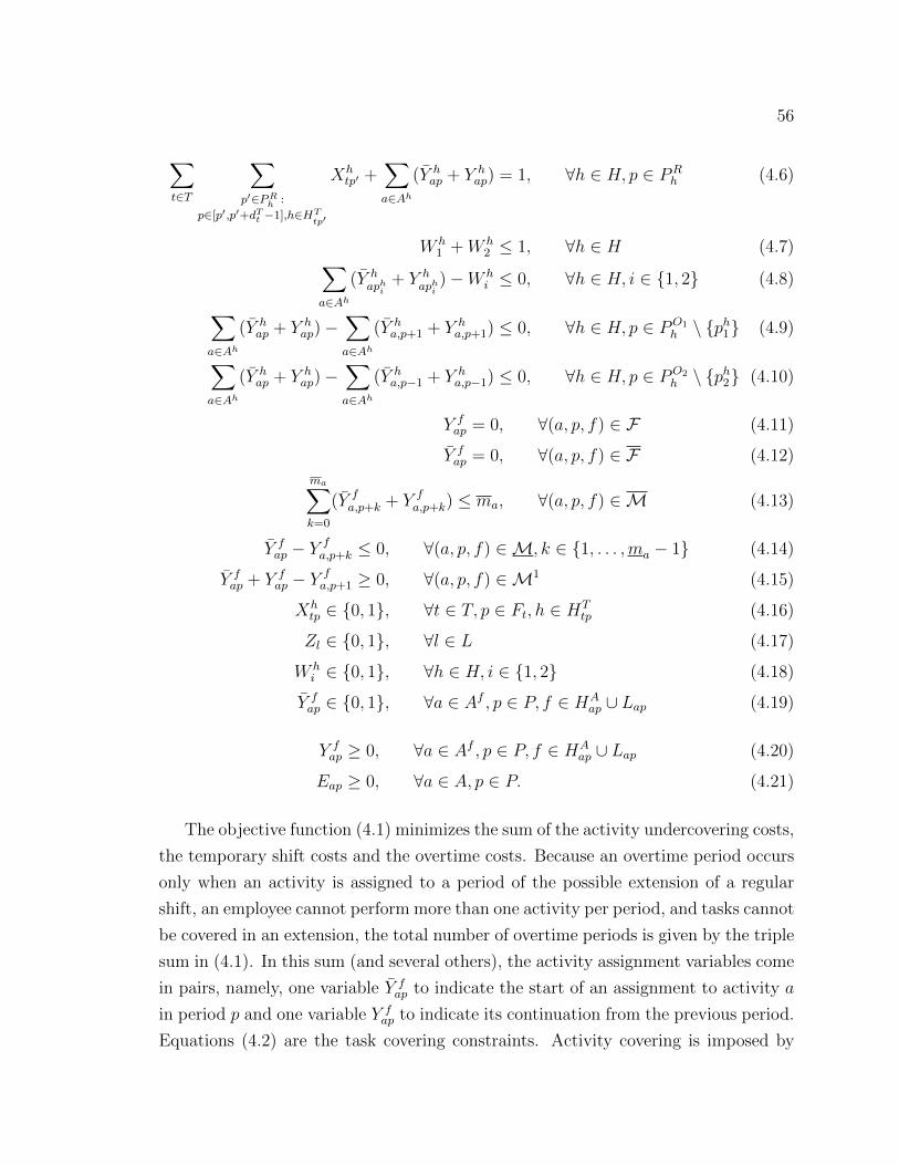
56

∑t∈T

∑p′∈PR

h :

p∈[p′,p′+dTt −1],h∈HTtp′

Xhtp′ +

∑a∈Ah

(Y hap + Y h

ap) = 1, ∀h ∈ H, p ∈ PRh (4.6)

W h1 +W h

2 ≤ 1, ∀h ∈ H (4.7)∑a∈Ah

(Y haphi

+ Y haphi

)−W hi ≤ 0, ∀h ∈ H, i ∈ 1, 2 (4.8)∑

a∈Ah

(Y hap + Y h

ap)−∑a∈Ah

(Y ha,p+1 + Y h

a,p+1) ≤ 0, ∀h ∈ H, p ∈ PO1h \ p

h1 (4.9)∑

a∈Ah

(Y hap + Y h

ap)−∑a∈Ah

(Y ha,p−1 + Y h

a,p−1) ≤ 0, ∀h ∈ H, p ∈ PO2h \ p

h2 (4.10)

Y fap = 0, ∀(a, p, f) ∈ F (4.11)

Y fap = 0, ∀(a, p, f) ∈ F (4.12)

ma∑k=0

(Y fa,p+k + Y f

a,p+k) ≤ ma, ∀(a, p, f) ∈M (4.13)

Y fap − Y

fa,p+k ≤ 0, ∀(a, p, f) ∈M, k ∈ 1, . . . ,ma − 1 (4.14)

Y fap + Y f

ap − Yfa,p+1 ≥ 0, ∀(a, p, f) ∈M1 (4.15)

Xhtp ∈ 0, 1, ∀t ∈ T, p ∈ Ft, h ∈ HT

tp (4.16)

Zl ∈ 0, 1, ∀l ∈ L (4.17)

W hi ∈ 0, 1, ∀h ∈ H, i ∈ 1, 2 (4.18)

Y fap ∈ 0, 1, ∀a ∈ Af , p ∈ P, f ∈ HA

ap ∪ Lap (4.19)

Y fap ≥ 0, ∀a ∈ Af , p ∈ P, f ∈ HA

ap ∪ Lap (4.20)

Eap ≥ 0, ∀a ∈ A, p ∈ P. (4.21)

The objective function (4.1) minimizes the sum of the activity undercovering costs,

the temporary shift costs and the overtime costs. Because an overtime period occurs

only when an activity is assigned to a period of the possible extension of a regular

shift, an employee cannot perform more than one activity per period, and tasks cannot

be covered in an extension, the total number of overtime periods is given by the triple

sum in (4.1). In this sum (and several others), the activity assignment variables come

in pairs, namely, one variable Y fap to indicate the start of an assignment to activity a

in period p and one variable Y fap to indicate its continuation from the previous period.

Equations (4.2) are the task covering constraints. Activity covering is imposed by

57

constraint set (4.3). Through the Eap variables, these constraints allow to compute

the number of activity undercoverings (that is, the shortage of employees with respect

to the demand) for each activity in each period. Inequalities (4.4) limit the number of

temporary shifts selected each day to the number of temporary employees available.

Constraints (4.5) force the rate of temporary working periods to total working periods

of all employees to fall within the desired range. In these constraints, the first, second

and third terms of the denominator provide the total numbers of periods worked

by the temporaries, by the regular employees in regular time, and by the regular

employees in overtime, respectively. Constraints (4.6) ensure that all segments of

the primary regular shifts are completely filled with activities or tasks. Based on

constraint set (4.7), at most one segment of each primary regular shift is extended.

By constraint set (4.8), activities can be assigned to the extension periods of a segment

only if the shift is extended on that segment. In case of extension, constraint sets (4.9)

and (4.10) impose the consecutivity of the extension periods.

Constraints (4.11) and (4.12) fix certain activity assignment variables to 0 (in

fact, these variables should not be defined but, to ease notation, it is simpler to set

them to 0). Because continuity of an assignment cannot occur in the first period of a

segment of a shift, all Y fap variables associated with these first periods are fixed to 0 in

constraints (4.11), where set F contains all triplets (a, p, f) ∈ A× P × (H ∪ L) such

that a ∈ Af and p is the first period of a segment in shift f (considering the possible

extension). Similarly, because it is not feasible to start an activity assignment too late

in a segment without violating the minimum assignment duration for this activity,

all Y fap variables associated with late periods in a segment are set to 0 in constraints

(4.12), where set F contains all triplets (a, p, f) ∈ A×P × (H ∪L) such that a ∈ Af

and p is a period such that the period p+ma − 1 falls outside the segment of shift f

containing p (including its extension).

Constraints (4.13) impose the maximum activity assignment durations by limiting

to ma the number of periods that an employee can be assigned to an activity a in

every set of ma + 1 consecutive periods. The set M contains all triplets (a, p, f) ∈A×P × (H ∪L) such that a ∈ Af and p is a period in shift f such that p and p+ma

belong to the same segment of f (including its possible extension). Constraints (4.14)

and (4.15) together force the minimum activity assignment durations. When the

assignment to an activity a starts in period p, this assignment must continue at least

for the next ma−1 periods as enforced by constraints (4.14). Furthermore, according

58

to constraints (4.15), an employee can continue to be assigned to an activity a in a

period p + 1 only if it was already assigned to it in period p. Set M (resp. M1)

contains all triplets (a, b, f) ∈ A × P × (H ∪ L) such that a ∈ Af and p is a period

in shift f such that p and p+ma − 1 (resp. p+ 1) belong to the same segment of f

(including its possible extension). Note that, to ease the solution of the first phase

model, the values of parameters ma and ma may be chosen to yield a relaxation of

the activity assignment duration constraints. For instance, if the minimum activity

duration is 4 periods for a given activity a, then one can set ma = 2 instead of ma = 4.

Finally, if the minimum assignment duration for an activity a ∈ A is equal to 1 in

the first phase (i.e., ma = 1), then all constraints (4.14) and (4.15) associated with a

can be discarded together with all Y fap variables.

At last, constraints (4.16)–(4.21) define the domains of the decision variables.

Notice that, to speed up the solution process, we relax the binary requirements on

the Y fap variables. In our computational experiments, we observe that they are often

satisfied by the computed solution (but not always).

Model (4.1)-(4.21) is solved using a commercial MIP solver. For our computa-

tional experiments, the exploration of the branch-and-bound search tree was stopped

either when a time limit of 1000 seconds is reached or when the difference between

the value of the current best solution and the current lower bound is less than cUc.

This tolerance was chosen because minimizing the total number of activity undercov-

erings is typically a priority and finding a solution with one additional undercovering

compared to an optimal solution is deemed acceptable.

4.2.2 Second phase

The second phase receives the following inputs from the first phase: a set of

potential temporary shifts with their start and end times; a set of potential regular

shift extensions; and the start time of each task and the shift to which it is assigned.

Starting from this information, the second phase aims at selecting which potential

temporary shifts and regular shift extensions to choose and assigning the activities

to the shifts considering the already assigned tasks. The output includes the regular

shifts’ new start and end times, as well as new break placements. Similar to AAFF

problem, we propose a column generation formulation for the second phase problem

and a heuristic branch-and-price rolling horizon procedure to solve it.

59

Column generation formulation for second phase problem

For each primary regular segment and each corresponding break start period, the

enumeration of all feasible segments including a possible extension and the assigned

activities are referred to as Segment Extension/Activity (SEA) assignments. Note

that the SEA assignments might include prefixed tasks. Also, for each temporary

shift, we assume that all possible activity assignments, which are referred to as AC-

Tivity (ACT) assignments, can be generated. In the second phase model, columns

correspond to SEA and ACT assignments. In addition to some of the notation pre-

viously defined in Section 3.2.1 and Section 4.2.1, the proposed column generation

model relies on the following notation.

Sets

L: Set of temporary shifts selected in the first phase.

Γl: Set of all feasible ACT assignments for temporary shift l ∈ L.

Parameters

csbω : Sum of the transition and overtime costs in SEA assignment ω ∈ Ωsb for segment

s ∈ S1 ∪ S2 with break start period b ∈ Bs.

clγ: Sum of the transition and temporary costs in ACT assignment γ ∈ Γl for tempo-

rary shift l ∈ L.

glγap: Binary coefficient equal to 1 if ACT assignment γ ∈ Γl for temporary shift l ∈ Lcovers activity a ∈ A during period p ∈ P , and 0 otherwise.

dsbω : Duration of segment s ∈ S1 ∪ S2 with break start period b ∈ Bs and SEA

assignment ω ∈ Ωsb.

Variables

∆lγ: Binary variable equal to 1 if ACT assignment γ ∈ Γl is selected for temporary

shift l ∈ L.

Using this notation, the second phase problem can be formulated as follows:

min cUc∑p∈P

∑a∈A

Eap +∑

s∈S1∪S2

∑b∈Bs

∑ω∈Ωsb

csbω Θsbω +

∑l∈L

∑γ∈Γl

clγ∆lγ (4.22)

60

s.t.:∑

s∈S1∪S2

∑b∈Bs

∑ω∈Ωsb

gsbωapΘsbω +

∑l∈L

∑γ∈Γl

glγap∆lγ + Eap ≥ nap,∀a ∈ A, p ∈ P (4.23)

∑ω∈Ωsb

∑b∈Bs

Θsbω = 1, ∀s ∈ S1 ∪ S2 (4.24)∑

γ∈Γl

∆lγ ≤ 1, ∀l ∈ L (4.25)

∑ω∈Ωsb

Θsbω −

∑ω∈Ωs′,b

Θs′,bω = 0, ∀(s, s′) ∈ H, b ∈ Bs (4.26)

rmin ≤

∑l∈L

∑γ∈Γl

dLl ∆lγ∑

l∈L

∑γ∈Γl

dLl ∆lγ +

∑s∈S1∪S2

∑b∈Bs

∑ω∈Ωsb

dsbω Θsbω

≤ rmax, (4.27)

Θsbω ∈ 0, 1 , ∀s ∈ S1 ∪ S2, b ∈ Bs, ω ∈ Ωsb (4.28)

∆lγ ∈ 0, 1 , ∀l ∈ L, γ ∈ Γl (4.29)

Eap ≥ 0, ∀a ∈ A, p ∈ P. (4.30)

Objective function (4.22) minimizes the total costs, including undercovering, over-

time, temporary and transition costs. Constraint set (4.23) sets up the number of

activity undercoverings for each period, resulting from the selected SEA and ACT

assignments. Constraints (4.24) ensures that a SEA assignment is assigned to each

regular shift segment. Constraint set (4.25) shows that we have the option to sched-

ule temporary employees among the shifts identified in the first phase, by selecting

ACT assignments for them. Constraint set (4.26) ensures the consecutivity of the

selected SEA assignment for the first segment, the meal break, and the selected SEA

assignment for the second segment forming a regular work shift. Constraints (4.27)

impose a lower and an upper bound on the rate of the temporary man-hours to the

total man-hours. Constraint sets (4.28)-(4.30) represent the domains of the variables.

Instead of constraint set (4.23), we use the equivalent constraint set (4.31) as

explained in Section 3.2.1.

61

∑s∈S1∪S2

∑b∈Bs

∑ω∈Ωsb

(gsbωap − gsbωa(p−1))Θsbω +

∑l∈L

∑γ∈Γl

(glγap − glγa(p−1))∆lγ

+Eap − Ea(p−1) = nap − na(p−1), ∀a ∈ A,∀p ∈ P .(4.31)

Rolling Horizon Procedure

While using the rolling horizon method for ATTFF, for a temporary shift in-

tersecting with a given time slice, all activity blocks assigned in the previous time

slice solution and ending prior to the start of the time slice are fixed. The same

adaptations and intersection kind definitions as described in Section 3.2.2 are used

for regular shifts here, although scheduled tasks from phase 1 are always kept even if

intersecting with the time slice. Also for temporary shifts the corresponding variables

are restricted to those of shifts intersecting with the time slice. Constraints (4.25) are,

however, transformed into equalities for every temporary shift with activity blocks

fixed from the previous time slices. This new constraints forces a temporary shift to

be scheduled in full, if a part of it is already assigned some activities in previous time

slices. Finally, constraints (4.27) need to be revised. Indeed, because they express an

overall requirement for the solution with respect to the entire planning horizon, they

lose consistency when they are used for an individual time slice. To satisfy the desired

bounds on the proportion of scheduled temporary work time to the total scheduled

work time, values within this range for each individual time slice may not be conclu-

sive for the entire horizon. Instead, we propose to use the temporary shifts selected

in the first phase as a guide to determine the proportion to use in each time slice.

More precisely, let r1 ∈ [rmin, rmax] be the rate (the value of the middle term in (4.5))

obtained from the first phase solution. Then, in each time slice, constraints (4.27)

are replaced by

rminr1

≤

∑l∈LIn

∑γ∈Γl

dLl ∆lγ +

∑l∈LSchBef

dLl∑l∈LUpToEnd

dLl≤ rmax

r1

, (4.32)

where LIn and LUpToEnd denote the subsets of temporary shifts considered in the

current time slice and from the start of the horizon up to the end of this slice,

62

respectively, whereas LSchBef indicates the temporary shifts scheduled in the previous

time slices. In the middle term of (4.32), the numerator (resp. denominator) is equal

to the total duration of the temporary shifts used in the second (resp. first) phase

solution up to the end of the current time slice. For example, if r1 = 5%, rmin = 3%

and rmax = 7%, then rmin

r1= 0.6 and rmax

r1= 1.4. Considering a time slice for which∑

l∈LSchBef

dLl = 30 and∑

l∈LUpToEnd

dLl = 60, then constraints (4.32) impose the scheduling

in the current time slice of temporary shifts whose total duration is between 6 and

54 periods (that is, such that [0.6, 1.4] = [30+660, 30+54

60]). Thus, they force the total

duration of all temporary shifts scheduled so far in the second phase to remain close

enough to the corresponding 60 temporary work periods assigned in the first phase

solution. Obviously, if LUpToEnd is empty for a time slice (which may happen in the

first time slices), then constraints (4.32) are omitted as no temporary shifts can be

scheduled in this time slice.

Because rmax

r1≥ 1.0 and the middle term of constraints (4.32) can never exceed 1.0,

upper bound rmax

r1is always satisfied and does not need to be considered. However,

this may not be the case when temporary shifts unused in the first phase solution can

also be selected as it will be possible in variants discussed in Section 4.2.3. Finally,

note that constraints (4.32) do not ensure that the minimum and maximum rates are

met. Indeed, the proportion of temporary work time over total work time depends

on the total number of overtime periods which, in these constraints, is assumed to

be equal in both phases. Because the number of overtime periods represents a small

fraction of the total scheduled work time and does not vary much between these

two phases, the approximation proposed in (4.32) seems acceptable. In fact, in our

computational experiments, the minimum and maximum rates were always satisfied.

If this was not the case, a (manual) adjustment of the solution could be performed.

Column generation heuristic

In the second phase, the master problem corresponds to the linear relaxation of

model (4.22), (4.24)–(4.26), (4.28)–(4.32), adapted to the current time slice. Besides

the dual variables πap, ∀a ∈ A, p ∈ P for constraints (4.31), τs, ∀s ∈ S1 ∪ S2 for

constraints (4.24) and λbs,s′ , ∀(s, s′) ∈ H, b ∈ Bs for constraints (4.26) defined in

Section 3.2.3 for the similar constraints, the additional dual variables are denoted as:

µl, ∀l ∈ L, for constraints (4.25) (or their equality counterparts); and

63

φmin and φmax for constraints (4.32).

There are two types of subproblems here. The first one corresponds to each segment

s ∈ S1In ∪ S2In and each possible break start time b ∈ BsIn. Let s ∈ S1In be the first

segment of a regular shift h ∈ H, b ∈ BsIn a break start period for s and ω ∈ Ωsb

In

a SEA assignment for s. Similar to the Section 3, the reduced cost csbω of the Θsbω

variables is given by:

csbω = csbω −∑a∈A

∑p∈P

(gsbωap − gsbωa(p−1))πap − τs − λbs,ρ2(s). (4.33)

Similarly, for the second segment s ∈ S2In of a regular shift h ∈ H and a break start

period b ∈ BsIn, the reduced cost csbω of a variable Θsb

ω , ω ∈ ΩsbIn is

csbω = csbω −∑a∈A

∑p∈P

(gsbωap − gsbωa(p−1))πap − τs + λbρ1(s),s. (4.34)

There is also a subproblem for every temporary shift involved in the current time

slice. If we denote by LIn the subset of subproblems for every temporary shift, let

l ∈ LIn be a temporary shift intersecting with the current time slice and denote by

ΓlIn the subset of its ACT assignments that are valid according to the intersection of

l with this time slice. The reduced cost clγ of a variable ∆lγ, γ ∈ ΓlIn is given by

clγ = clγ −∑a∈AL

∑p∈P

(glγap − glγa(p−1))πap − µl −dLl∑

l∈LUpToEnd

dLl(φmin + φmax). (4.35)

Thus, the subproblem for shift l is defined as

minγ∈Γl

In

clγ.

where its constraints appear in the definition of set ΓlIn.

The definition of subproblems for regular shift segments is similar to what was

described in Section 3.2.3. In the ATTFF problem, there may also be a subset of tasks

preassigned to segment s, denoted by T s. Up to two types of nodes can be added

to the network in this problem. 1) A start of task node Bt,pt and 2) an end of task

node Et,pt+dTt −1 for each preassigned task t ∈ T s that starts in period pt (according

to the first phase solution). Such a network can contain an additional arc type for

64

scheduled tasks compared to networks in AAFF problem.

The arcs for networks corresponding to segment s ∈ S1In ∪ S2In of regular shift

h ∈ H and break start period b ∈ BsIn are defined in Table 4.1.

Table 4.1 Definition of arcs in subproblem of segment s ∈ S1In ∪ S2In

Type Origin Destination Cost1 α Ba,p,∀a ∈ Ah,

Btp, ∀t ∈ T s,s ∈ S1In : p ∈ QsbIn,s ∈ S2In : p = b+ q,

s ∈ S1In : −τs − λbs,ρ2(s)+cOvt(ph1 + 1− p),s ∈ S2In : −τs + λbρ1(s),s

2 Ea,p,∀a ∈ Ah,Etp, ∀t ∈ T s,s ∈ S1In : p = b−1,s ∈ S2In : p ∈ QsbIn

β s ∈ S1In : 0,s ∈ S2In : cOvt(p−ph2 +1)

3 Ba,p,∀a ∈ Ah,∀p ∈ P sbIn

Ea,p+j−1,dmina ≤ j ≤ dmaxa ,p+ j − 1 ∈ P sbIn,[p, p+ j − 1] ∩ [pfd , p

td] =

∅,∀d ∈ DsbIn,

[p, p+ j − 1] ∩ [pt, pt + dTt − 1] =∅,∀t ∈ T s,

πa,p+j − πa,p

4 Ea,p,∀a ∈ Ah,s ∈ S1In :∀p ∈ P sbIn \ b− 1,s ∈ S2In :∀p ∈ P sbIn \ ph2

Ba′,p+1,∀a′ ∈ Ah\a,Bt,p+1, ∀t ∈ T s

cTrs

Et,p, ∀t ∈ T s Ba,p+1,∀a ∈ Ah,Bt′,p+1,∀t′ ∈ T s \ t

5 Badpfd,

∀d ∈ DsbIn

Eadptd , 0

6 Bt,pt ,∀t ∈ T s

Et,pt+dTt −1 0

For definition of the subproblem for temporary shift l ∈ LIn, denote by stl the

start period of shift l, and by DlIn the set of preassigned activity blocks for temporary

shift l. A preassigned activity block d ∈ DlIn corresponds to activity type ad starting

at period pfd and ending at period ptd. The corresponding network has the same types

of nodes and arcs as in Section 3.2.3. The costs on arcs are defined in Table 4.2.

Depending on the intersection kind for regular shifts, complementary subproblems

generate the columns for assignments corresponding to first and second segments

sharing the same break start period based on Algorithm 1 at each column generation

65

Table 4.2 Arc definition for temporary shift l ∈ L

Type Origin Destination Cost1 α Ba,stl ,∀a ∈ Al cTmpdLl − µl

− dLl∑l∈LUpToEnd

dLl(φmin + φmax)

2 Ea,stl+dLl ,∀a ∈ Al β 0

3 Ba,p,∀a ∈ Al,∀p ∈ [stl, stl + dLl ]

Ea,p+j−1,dmina ≤ j ≤ dmaxa ,p+ j − 1 ∈ [st− l, stl + dLl ],

[p, p+ j − 1] ∩ [pfd , ptd] =

∅,∀d ∈ DlIn

πa,p+j − πa,p

4 Ea,p,∀a ∈ Al,∀p ∈ [stl, stl + dLl − 1]

Ba′,p+1,∀a′ ∈ Al\a cTrs

5 Badpfd,

∀d ∈ DlIn

Eadptd , 0

iteration. It is already decided in phase one which segments can have extensions. If

we denote these segments by set Sext, the subset of periods QsbIn is equal to Qsb, for

segments s ∈ Sext, and includes only the primary start/end of the shift otherwise. In

second phase, the break starts which require an extension to a segment s /∈ Sext are

removed from Bs. In other words, for segments s /∈ S1 ∩ Sext we solve subproblems

only with break starts b ∈ Bs \ b | ph1 + 1 /∈ Qsb, and for segments s /∈ S2 ∩ Sext

only with break starts b ∈ Bs \ b | ph2 − 1 /∈ Qsb. For each temporary shift, a single

column is generated based on Algorithm 2 at each column generation iteration.

Algorithm 2 Solving the subproblem for temporary shifts

1: for all temporary shift l ∈ LIn do2: Solve the subproblem for shift l.3: if the least reduced cost column found has a negative reduced cost then4: Add this column to RMP

The rounding procedure described in Section 3.2.3 is used here at the end of each

column generation procedure for fractional-valued variables ∆lγ as well as Θsb

ω .

66

4.2.3 Variants

The proposed two-phase method can easily be modified to yield variants that

differ in the flexibility options considered. In these variants, In our computational

experiments, we used the following six variants.

Variant ext-tmp allows break movements, and regular shift extensions and temporary

employees identified in the first phase. It uses the two-phase method described

above.

Variant no allows no flexibility at all (that is, no temporary shifts, no shift extensions,

and no break movements). For this variant, Both phases’ models are simplified

by removing all aspects related to temporary shifts, regular shift extensions,

and break movements.

Variant ext allows only break movements and regular shift extensions. In this case,

all aspects related to the temporary shifts are omitted from both phases’ models.

Variant allext is the same as ext except that all possible extensions are considered in

the second phase. This variant solves an AAFF problem with preassigned tasks

in phase 2. In this case, the first phase still schedules and assigns the tasks taking

into account the possibility of extending the regular shifts. In the second phase,

additional constraints (3.5) stipulating that at most one extension can occur

per regular shift must be added to model (4.22),(4.24)–(4.26), (4.28)–(4.32).

Furthermore, the networks for all the subproblems associated with the regular

shift segments include the possibility to extend the corresponding segment.

Variant ext-alltmp is the same as ext-tmp except that all temporary shifts (not only

those selected in the first phase solution) are considered in the second phase.

In this case, the first phase remains unchanged. In the second phase, the upper

bound constraint (4.32) as well as the following additional sets of constraints

limiting the number of temporary shifts per day are also taken into account:∑l∈Lj

In

∑γ∈Γl

∆lγ + |LjSchBef | ≤ κj, ∀j ∈ J In (4.36)

where J In denotes the subset of days covered by the current time slice, LjIndenotes the subset of temporary shifts considered in the current time slice and

belonging to day j ∈ J In, and LjSchBef denotes the subset of temporary shifts

67

belonging to day j ∈ J In which are scheduled in the previous time slice. Ac-

cordingly, in order to avoid infeasibility corresponding the constraints (4.36) the

rounding procedure for temporary shift assignment variables stops after the fol-

lowing equality is reached. Denote by Lfixed the subset of temporary shifts for

which either an ACT assignment variable is selected by the rounding procedure

of the current time slice so far or have activity blocks fixed from the previous

time slices:

|Lfixed|+ |LjSchBef | = κj. (4.37)

In order to avoid infeasibility due to the upper bound of constraints (4.32), a

∆l′γ variable is only rounded to 1 if temporary shift l′ satisfies the following

constraint: ∑l∈Lfixed

dLl + dLl′ +∑

l∈LSchBef

dLl∑l∈LUpToEnd

dLl≤ rmax

r1

. (4.38)

If shift l′ has activity blocks fixed from the previous time slices, no limitation

is put for fixing a schedule for that.

Variant nobrkmv is the same as ext-tmp, except that break movements are not

allowed. Consequently, in the second phase, the break of every primary regular

shift is fixed and there is a single subproblem per segment of each of these shifts.

4.3 COMPUTATIONAL RESULTS

We tested the six variants of the two-phase heuristic on two classes of medium-

and large-sized instances. Each class includes 5 randomly generated instances. In the

first class, the instances are defined over a one-day horizon and involve 50 regular

employees and 5 temporary employees to be assigned to 10 tasks and 10 different

activities. In the second class, they are defined over a one-week horizon (7 days) and

involve 30 regular employees working each 4 or 5 days during the week, 3 temporary

employees available per day, 35 tasks and 6 activities. The set L of the temporary

shifts is composed of all shifts of durations 3, 4 and 5 hours, starting on the hour

at every hour every day of the horizon such that it starts after 6am and ends before

68

11pm. Two copies of each shift are included in L, giving the possibility to assign

a maximum of two temporary employees to the same shift (this seems sufficient in

practice and limits the size of the first phase model). In total, there are 2 × 42 and

2 × 294 temporary shifts for the one-day and one-week instances, respectively. The

minimum and maximum durations of a segment are 195 and 300 minutes, respectively.

For all activities, the minimum and maximum activity assignment durations are 60

and 180 minutes, respectively. The duration of the tasks varies between 30 and 180

minutes. For each instance, two scenarios of demands are considered, denoted D1

and D2. The second scenario differs from the first one only by an increased demand

(around 5% and 10% higher for the first and the second class, respectively) for the

activities that can be performed by the temporaries. The other parameters were set as

follows: rmin = 3%, rmax = 7%, cUc = 165, cOvt = 45, cTmp = 30, and cTrs = 2. With

these values, extending a shift by 45 minutes (3 periods) is profitable if it saves at least

one undercovering. On the other hand, extending it by 60 minutes is not worth it if

only one or no undercovering is saved. Also, scheduling a 3, 4 or 5-hour temporary

shift is worthwhile if it saves at least 3, 3 or 4 undercoverings, respectively. Thus,

this cost structure highly favors the minimization of the number of undercoverings.

For the first class instances, we did not apply the rolling horizon procedure in the

second phase, that is, model (4.22),(4.24)–(4.26), (4.28)–(4.32) was solved at once

using the column generation heuristic. For the second class, the length of a time

slice was set to 4320 minutes (3 days) and the consecutive time slices overlapped by

1440 minutes (1 day). For our tests, we used the Xpress-MP solver (version 7.2.1)

of the Fair Isaac Corporation for solving all linear and integer programs. All our

experiments were conducted on an Intel R©CoreTMi7-2600 processor (using a single

CPU) clocked at 3.4GHz with 16GB RAM.

We conducted two series of computational experiments. The first aims at assessing

the quality of the solutions produced by the proposed two-phase solution method for

the nobrkmv variant. The second compares different flexibility combinations.

4.3.1 Solution quality for the nobrkmv variant

To assess the quality of the solutions computed by the two-phase heuristic, one

can compute lower bounds using a relaxation of the ATTFF. Assuming that the

tasks cannot be performed during overtime, the first phase model (4.1)–(4.21) is a

relaxation of the ATTFF when no break movements are allowed, that is, for the

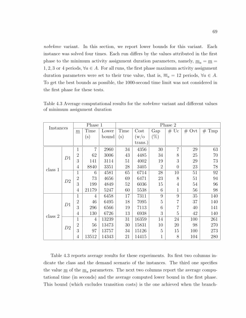
69

nobrkmv variant. In this section, we report lower bounds for this variant. Each

instance was solved four times. Each run differs by the values attributed in the first

phase to the minimum activity assignment duration parameters, namely, ma = m =

1, 2, 3 or 4 periods, ∀a ∈ A. For all runs, the first phase maximum activity assignment

duration parameters were set to their true value, that is, ma = 12 periods, ∀a ∈ A.

To get the best bounds as possible, the 1000-second time limit was not considered in

the first phase for these tests.

Table 4.3 Average computational results for the nobrkmv variant and different valuesof minimum assignment duration

InstancesPhase 1 Phase 2

m Time(s)

Lowerbound

Time(s)

Cost(w/otrans.)

Gap(%)

# Uc # Ovt # Tmp

class 1

D1

1 7 2960 34 4356 30 7 29 632 62 3006 43 4485 34 8 25 703 141 3114 51 4002 19 3 29 734 8840 3351 28 3405 2 0 23 78

D2

1 6 4581 65 6714 28 10 51 922 73 4656 69 6471 23 8 51 943 199 4849 52 6036 15 4 54 964 21179 5247 60 5538 6 1 56 98

class 2

D1

1 4 6458 17 7311 9 9 35 1402 46 6495 18 7095 5 7 37 1403 296 6566 19 7113 6 7 40 1414 130 6726 13 6938 3 5 42 140

D2

1 4 13239 31 16359 14 24 100 2612 56 13473 30 15831 10 20 98 2703 97 13757 34 15126 5 15 100 2734 13512 14343 21 14415 1 8 104 280

Table 4.3 reports average results for these experiments. Its first two columns in-

dicate the class and the demand scenario of the instances. The third one specifies

the value m of the ma parameters. The next two columns report the average compu-

tational time (in seconds) and the average computed lower bound in the first phase.

This bound (which excludes transition costs) is the one achieved when the branch-

70

and-bound process stops and may be lower than the cost of the best feasible solution

found (recall that the search tree exploration can be prematurely stopped; see end of

Section 4.2.1). The last six columns provide average results for the second phase: the

computational time (in seconds), the cost of the computed solution excluding also the

transition costs, the gap (in percentage) between the solution cost and the best lower

bound found (i.e., with m = 4), the total number of activity undercoverings (# Uc),

the total number of periods in overtime (# Ovt), and the total number of periods in

the scheduled temporary shifts (# Tmp). Because transition costs are not considered

in the first phase, we do not report them in the second phase solution costs (although

they were considered during optimization). All averages were computed over five

instances.

For the first phase, these results show that, as expected, increasing the value of

m improves the quality of the average lower bound. In fact, this improvement varies

between 4% and 15% for the different pairs of class and demand scenario. Unfortu-

nately, we observe that the average computational time also increases significantly.

This time increase is more drastic for the 1-day instances (class 1): when m = 4,

half of the 10 instances required more than 10,000 seconds. For the second phase, we

observe that the average computational time is relatively constant with respect to m.

However, when m increases, the solution cost and the gap decrease, showing that the

first phase solution provides better information to the second phase when m is larger.

We notice that the average gaps are very low for m = 4. However, for this case, the

total computational time (including the time required in the first phase) may be too

large. Consequently, to produce the results presented in the next section, we used

m = 3 that provided reasonable computational times. In Table 4.3, this value yielded

average gaps varying between 5% and 19%, which may seem relatively large. Note

however that the objective function considered does not take into account the cost of

the periods worked in regular time in the regular shifts. Accounting for such a cost

(say, 30 per period as for a temporary worker) would rather yield gaps smaller than

1.6%, which would be highly acceptable.

4.3.2 Flexibility combinations

The purpose of our second series of experiments was to compare different flexibility

combinations (variants no, ext, ext-tmp and nobrkmv) by evaluating their effect on

activity assignment decisions and on the computational time of the proposed solution

71

method. To assess the quality of the solutions produced by variants ext and ext-tmp,

we also tested the variants allext and ext-alltmp which should produce better quality

solutions as they allow more flexibility in the second phase. On the other hand, these

variants are more computationally extensive.

Table 4.4 reports the average computational results obtained for each instance

class and demand scenario by each solution method variant. In this table, the first

three columns indicate the class and the demand scenario of the instances and the

solution method variant used. The other columns display averages over the five

instances of each pair of class and demand scenario: the computational time (in

seconds) for each phase and in total, the solution cost (including transition costs),

the total number of activity undercoverings (# Uc), the total number of periods

in overtime (# Ovt), the total number of periods in scheduled temporary shifts (#

Tmp), and its percentage with respect to the total number of periods worked by all

employees (% Tmp).

From the average results, we make the following observations. First, comparing the

number of undercoverings (the main part of the objective function) obtained by the

no variant with the other three flexibility levels (ext, ext-tmp and nobrkmv variants)

clearly shows the coverage improvements that can be achieved by using flexibilities.

In fact, with the ext-tmp option, the number of undercoverings is reduced on average

by 95%, while maintaining reasonable computational times (on average between 5 and

14 minutes). Using solely segment extensions (ext variant) also allows a significant

reduction in the number of undercoverings in acceptable computational times (on

average between 3 and 22 minutes). Comparing the total costs, we remark that using

temporaries is profitable on average for all classes and demand levels (average savings

of 27% when compared to the solutions of the ext variant, respectively). This is not

the case, however, for a few individual instances where the number of undercoverings

saved by using temporaries does not outweight their costs which are unavoidable to

reach the minimum proportion of working time assigned to the temporaries. The last

column indicates that, on average, the rmin and rmax bounds on this proportion are

respected (in fact, they are satisfied by the solution of each instance). Obviously,

the amount of work periods assigned to temporaries is higher for demand level D2.

However, as expected, the number of undercoverings is higher for demand scenario

D2 than for scenario D1.

The results for the nobrkmv variant allow to assess the impact of moving breaks.

72

Table 4.4 Average computational results for all variants

Instances Variant Timephase1 (s)

Timephase2 (s)

Totaltime(s)

Cost #Uc

#Ovt

#Tmp

%Tmp

class 1

D1

no 29 83 112 11637 81 - - -ext 101 1211 1312 5354 9 78 - -

ext-tmp 141 428 569 4012 3 24 70 4.5nobrkmv 141 51 192 4282 3 29 73 4.6

allext 29 4165 4194 4630 5 80 - -ext-alltmp 141 743 884 4007 4 16 80 5.1

D2

no 18 46 64 21352 128 - - -ext 120 750 870 8614 14 132 - -

ext-tmp 199 643 842 6553 6 52 96 5.9nobrkmv 199 52 251 6334 4 54 96 5.9

allext 18 2855 2873 9144 17 134 - -ext-alltmp 199 748 947 6611 7 49 100 6.1

class 2

D1

no 231 84 315 14596 85 - - -ext 26 160 186 8344 29 66 - -

ext-tmp 258 149 408 6784 5 28 138 3.3nobrkmv 258 20 278 7735 6 40 142 3.4

allext 231 448 679 7808 24 73 - -ext-alltmp 258 355 613 6748 3 28 144 3.4

D2

no 306 60 366 42732 255 - - -ext 33 231 264 24495 93 189 - -

ext-tmp 97 206 303 14302 10 86 273 6.2nobrkmv 97 34 131 15785 15 100 273 6.2

allext 306 732 1038 23254 80 202 - -ext-alltmp 97 900 998 14912 14 76 283 6.5

73

Compared to the results of the ext-tmp variant, we observe an average reduction of

6.1% in the cost of the solution computed when break repositioning is considered (ext-

tmp variant). On the other hand, allowing break movements increases the average

computational time by a factor varying between 1.4 and 3.4. This increase is caused

by the large number of column generation subproblems considered in the second phase

when breaks can be moved.

Now, let us compare the results of variants allext and ext-alltmp with those of

variants ext and ext-tmp. We observe that allowing all extensions in the second phase

(variant allext) yields an average cost reduction of 4.7% compared to the ext variant

while allowing all temporary shifts (variant ext-alltmp) provides more or less the same

average solution cost as that derived with the ext-tmp variant. This shows that the

first phase performs well for selecting the temporary shifts but could be more accurate

for selecting the possible extensions. Given that the ext and ext-tmp variants require

much less computational time than their counterparts (they are on average 3.5 and

1.9 times faster), these two variants offer a good trade-off between solution quality

and total computational time.

Notice that the average computational time is less for the one-week instances

(class 2) than for the one-day instances (class 1) even if the former are much larger

in size than the latter. This is due to the rolling horizon procedure that is used for

the one-week instances and allows to control efficiently the computational time.

4.3.3 Conclusion

To overcome the complexities of the previous chapter problem, an efficient two-

phase heuristic is developed to compute good solutions for large-sized instances within

practical computational times. The solution approach developed at the beginning

of the work is using an approximate mixed-integer programming model in the first

phase to reduce the search space. Besides, the previous chapter model is extended

to also consider some more features and flexibilities. These include scheduling some

tasks before their due dates in a way that brings the least shortage of employees

to cover the activities demands. Each task needs just one qualified empolyee to

start it once and finish it without interruption. To even better help covering the

activities in this situation temporary employees can be called in. Given preassigned

tasks, potential temporary shifts and potential overtime periods for regular shifts,

all suggested by the first phase solution, the second phase computes a final solution

74

using an extended column generation formulation and heuristic embedded into a

rolling horizon procedure. This heuristic was tested on randomly generated medium-

to large-sized instances to compare different variants of flexibility.

The computational results show that the additional flexibilities can yield substan-

tial savings in the number of activity demand undercoverings and that the solutions

can be computed in reasonable computational times. To asses the quality of final

solutions the idea of adding the nobrkmv variant (considering all flexibilities except

for break repositioning) was originated. Knowing that break movements are not

considered in the first-phase approximation model, for this variant the value of the

first-phase solution serves as a lower bound for the final solution of the second phase.

The article ”A two-phase mathematical-programming heuristic for flexible assign-

ment of activities”, written by Mahsa Elahipanah, Guy Desaulniers and Eve Lacasse-

Guay, consisting of a summary of the contents of this chapter was submitted for

publication to Journal of Scheduling in May 2011.

75

CHAPTER 5

A TWO-PHASE BRANCH-AND-PRICE HEURISTIC FOR

PREFERENCE BASED ACTIVITY ASSIGNMENT TO WORK

SHIFTS

5.1 PREFERENCE-BASED ACTIVITY ASSIGNMENT (PBAA)

In the PBAA problem, there are some regular full-time shifts with known start

and end times, break positions and assigned employees. Each employee indicates a

level of high, low or no pereference for performing each activity he is qualified for. The

purpose is to assign activities to employee work shifts based on their qualifications

and the duration bounds on the activity assignments. We look for the assignments

which optimize three hierarchical objective functions. The most important objective

aims at minimizing undercovering costs. After that, the selected assignments should

also maximize the satisfaction of employees. Finally the incurred transition costs by

the selected assignments should be minimized. A satisfaction rate measure is going

to be defined in Section 5.1.1, for evaluating each employee satisfaction. The second

objective is then defined as maximizing the average satisfaction rate for employees

(or, equivalently, minimizing its negative value).

Defining a single model for the PBAA problem is not simple, because including

three hierarchical levels in one objective function is not always easy. On the one

hand, it requires choosing the importance factors for each of these levels, which has

some drawbacks in practice. On the other hand, since these measures have different

units and dimensions, normalization of measures is required to correctly translate the

importance factors, given by the decision maker, to the final weights. Choosing and

applying a normalization method itself has its own difficulties.

The PBAA problem is, by nature, a multi-objective problem with conflicting ob-

jectives. This means that the improvement in one objective results in the decline in

the others. For example, minimizing undercovering might be conflicting with max-

imizing preference satisfaction. This kind of problems does not have an optimal

solution but rather a set of Pareto-optimal (non-dominated) solutions, none of which

has a dominant value for all the objectives. A common solution method for such a

76

problem consists of transforming it into a problem with a single objective, like the

weighting method explained in Sectoin 2.3.1, and then trying to find or estimate the

Pareto-optimal solutions by using different combination of weights for the objectives.

In the PBAA problem, the priority is with the demand coverage as the first objec-

tive. Only small violations from the minimum undercovering costs can be accepted,

in hopes of gaining higher satisfaction average for employees. The purpose of this

chapter is to propose a two-phase method, which considers the objectives separately

in a hierarchical way, and to test its efficiency and applicability in comparison with

the one-phase weighting method.

A schematic description of the PBAA multi-objective optimization problem is

given in Figure 5.1, showing the relationship between the first two objectives. The

horizontal and vertical axes show the values of the undercovering cost and employee

satisfaction rate average objectives, respectively. The curve on top is the optimal

Pareto-front, while the one in the bottom gives an estimation of that. This estima-

tion results from different pairs of values within their corresponding objective range,

obtained by a heuristic method. The minimum possible undercovering cost, as well

as the maximum possible satisfaction rate average are distinguished on the extremi-

ties of the optimal Pareto-front. By moving along the curve from the minimum cost

point we can reach the solutions with higher average satisfaction rate, while the un-

dercovering cost is increased. In the PBAA problem we are interested in estimating

the lower part of the Pareto-front curve close to the minimum cost solution, marked

with an oval on the figure. The reason is that the solutions which are violating the

minimum cost by a sma‘ll percentage but include the more satisfactory assignments

for employees might be also interesting.5.1.1 Measuring employee satisfaction rate

Bonus Bhigh is considered for a one-period assignment of a high-preference activity

to an employee, while bonus Blow presents a low-preference activity assignment to

employees. No bonus is considered for the assignment of no-preference activities.

The following notation is used to define the employee satisfaction measure.

SetsE: Set of employees.

Ae: Subset of activities a ∈ A employee e ∈ E is skilled for.

Aelow: Subset of activities a ∈ Ae categorized as low-preference for employee e ∈ E.

Aehigh: Subset of activities a ∈ Ae categorized as high-preference for employee e ∈ E.

77

Undercovering cost

Satisfaction rate average

Figure 5.1 Multi-objective optimization

S: Set of all segments in the planning horizon.

Se: Subset of segments s ∈ S corresponding to employee e.

Spe : Subset of segments s ∈ Se beginning not later than period p ∈ P .

P s: Subset of periods p ∈ P covered by segment s ∈ S.

Ωs: Set of all feasible activity assignments for segment s ∈ S.

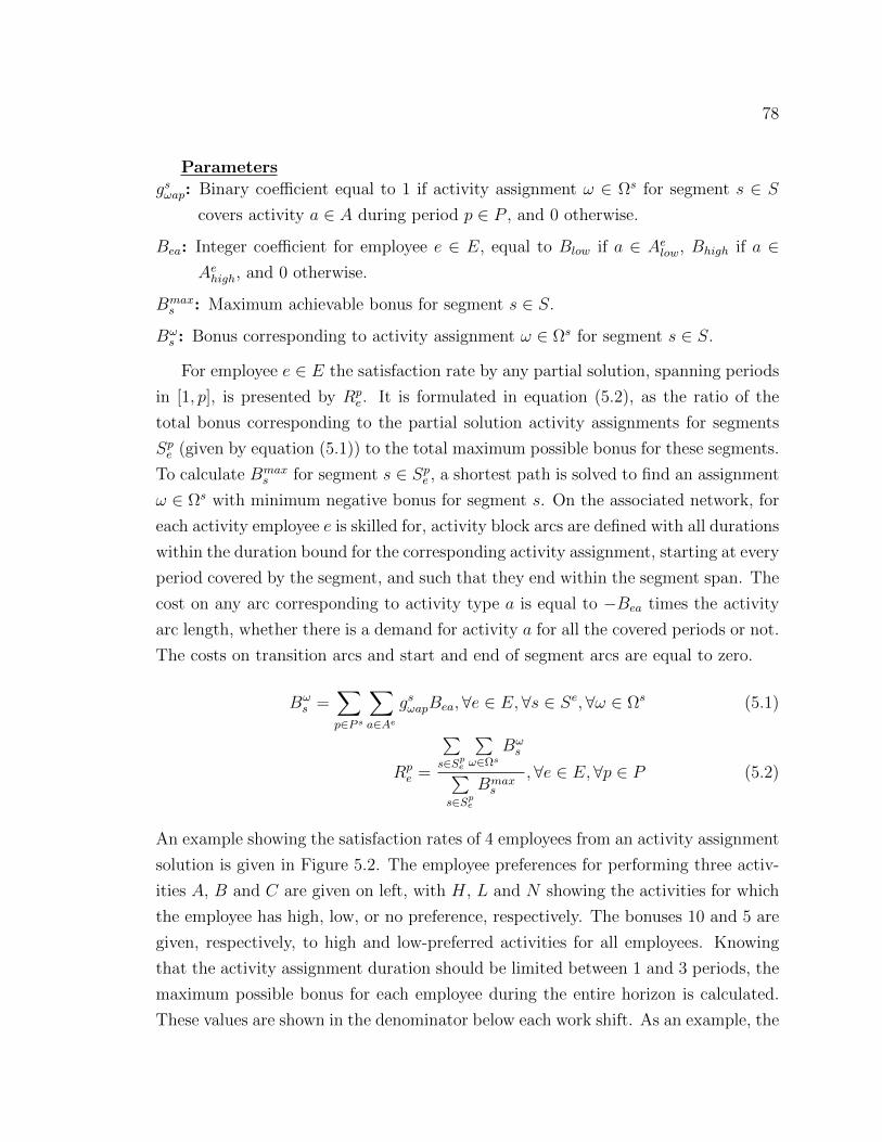
78

Parameters

gsωap: Binary coefficient equal to 1 if activity assignment ω ∈ Ωs for segment s ∈ Scovers activity a ∈ A during period p ∈ P , and 0 otherwise.

Bea: Integer coefficient for employee e ∈ E, equal to Blow if a ∈ Aelow, Bhigh if a ∈Aehigh, and 0 otherwise.

Bmaxs : Maximum achievable bonus for segment s ∈ S.

Bωs : Bonus corresponding to activity assignment ω ∈ Ωs for segment s ∈ S.

For employee e ∈ E the satisfaction rate by any partial solution, spanning periods

in [1, p], is presented by Rpe. It is formulated in equation (5.2), as the ratio of the

total bonus corresponding to the partial solution activity assignments for segments

Spe (given by equation (5.1)) to the total maximum possible bonus for these segments.

To calculate Bmaxs for segment s ∈ Spe , a shortest path is solved to find an assignment

ω ∈ Ωs with minimum negative bonus for segment s. On the associated network, for

each activity employee e is skilled for, activity block arcs are defined with all durations

within the duration bound for the corresponding activity assignment, starting at every

period covered by the segment, and such that they end within the segment span. The

cost on any arc corresponding to activity type a is equal to −Bea times the activity

arc length, whether there is a demand for activity a for all the covered periods or not.

The costs on transition arcs and start and end of segment arcs are equal to zero.

Bωs =

∑p∈P s

∑a∈Ae

gsωapBea,∀e ∈ E,∀s ∈ Se,∀ω ∈ Ωs (5.1)

Rpe =

∑s∈Sp

e

∑ω∈Ωs

Bωs∑

s∈Spe

Bmaxs

,∀e ∈ E,∀p ∈ P (5.2)

An example showing the satisfaction rates of 4 employees from an activity assignment

solution is given in Figure 5.2. The employee preferences for performing three activ-

ities A, B and C are given on left, with H, L and N showing the activities for which

the employee has high, low, or no preference, respectively. The bonuses 10 and 5 are

given, respectively, to high and low-preferred activities for all employees. Knowing

that the activity assignment duration should be limited between 1 and 3 periods, the

maximum possible bonus for each employee during the entire horizon is calculated.

These values are shown in the denominator below each work shift. As an example, the

79

network for obtaining the maximum possible (or minimum negative) bonus for the

first segment of employee 2 is illustrated in Figure 5.3, with the shortest path leading

to this value represented with solid arrows. For the illustrated activity assignment

solution in Figure 5.2, the achieved bonus for each work shift is also calculated, as

shown in the numerator below them. As a result, the satisfaction of each employee

is calculated as the given ratio.

1 2 3 4 5 6 7 8 9 10 11 12 13 14

A B B A

A B B

C A

A A B

1

2

3

4

time

A

C

B

C A

B

(10) (5) (0)

A C B

A B C

C B A

B C A

preferences

= 29%

H L N

10+ 10+ 0 + 0 + 10 + 0 + 0 + 0

10+ 10 + 0 + 5 + 0 + 0 = 50%

= 50%

= 46%

0 + 10 + 0 + 0 + 0 + 5 + 0 + 5 + 5 + 0

0 + 0 + 5 + 10 + 0 + 10+ 10 + 0 + 0

Min. Activity duration=1 period

Max. Activity duration=3 periods

10+ 10+ 10 + 0 + 10 + 10+ 10 + 5

10+ 10 + 0 + 10 + 10+ 10

10+ 10+ 10 + 5 + 10+ 10 + 0 + 10+ 10 +10

10+10+ 10 + 5 + 0 + 10+ 10 + 10+ 5

employees

Figure 5.2 Example of satisfaction rates for an activity assignment

C β

E23

E13

B13

B23

E22

E12

B12

B22

A(0) E11

B11

E23

E13

B13

B23

E14

B14

E25

E15

B15

B25

E26

E16

B16

B26B(5)

C(10) E23

B23

E32

B32

B31

E33

B33

E34

B34

E35

B35

E36

B36

E21

E31

α

B21

­3*10

­1*5B

24E

24

­2*10

Figure 5.3 Shortest path network for first segment of employee 2

80

5.2 MODEL FOR THE ONE-PHASE METHOD

We propose a one-phase method to solve the PBAA problem with a multi-objective

activity assignment. This method relies on a column generation (CG) model, in which

columns correspond to possible activity assignment combinations for each segment

without the flexibilities considered in the two previous chapters. Accordingly, Θsω is

a binary variable equal to 1 if activity assignment ω ∈ Ωs is selected for segment

s ∈ S, and 0 otherwise. In this method, a single objective function is used, which

combines the three objectives together, with a large importance weight given to the

undercovering measure, a moderate weight to the employee satisfaction measure, and

a small weight to the transition measure. To get the desired solutions with undercov-

ering costs close to the optimum, specifying the weigths in the one-phase method is a

difficult task. By applying this method, we try to find a number of the Pareto-optimal

solutions with slightly violated minimum undercovering costs, by several runs with

different combination of weights. One of the disadvantages of the one-phase method

could be the difficulty of setting a set of weights which works efficiently for different

sets of instances.

The weighted-sum model is formulated as follows, while csω presents the transition

cost in activity assignment ω ∈ Ωs for segment s ∈ S, and cUca stands for the cost of an

undercovering for activity a ∈ A. Also denoting by J = 1, 2, 3 the set of objectives

(showing respectively the undercovering cost, employee satisfaction and transition

cost objectives), w1j denotes the weight given by decision-maker to objective j ∈ Jin the one-phase method. Finally, the same definitions given in Section 3.2.1 apply

for Eap and nap.

min w11

∑a∈A

cUca∑p∈P

Eap − w12

∑e∈E

∑s∈Se

∑ω∈Ωs

Bωs Θs

ω∑s∈Se

Bmaxs

+ w13

∑s∈S

∑ω∈Ωs

csωΘsω (5.3)

s.t.:∑s∈S

∑ω∈Ωs

(gsωap − gsωa(p−1))Θsω + Eap − Ea(p−1)

= nap − na(p−1), ∀a ∈ A,∀p ∈ P (5.4)∑ω∈Ωs

Θsω = 1, ∀s ∈ S (5.5)

Θsω ∈ 0, 1 , ∀s ∈ S, ω ∈ Ωs (5.6)

Eap ≥ 0, ∀a ∈ A, p ∈ P. (5.7)

81

The constraints (5.4)–(5.7) are similarly used in the formulation of the AAFF

problem in Section 3.2.1. Constraint set (5.4) sets up the number of activity under-

coverings for each period, resulting from the selected assignments. These constraints

are transformed to reduce the constraint matrix density, as explained in Section 3.2.1.

Constraints(5.5) ensure that an assignment is selected for each segment. Constraint

sets (5.6)–(5.7) represent the domain of variables. Note that the second term in the

objective function, with the minus sign, corresponds to the minimization of a negative

value, which is equivalent to maximizing the average satisfaction rate. In calculating

the average satisfaction rate, the sum of satisfaction rates should be divided by the

number of employees. Since it corresponds to a division by a constant number, it is

omitted from the second term.

This model and the models to be described for the two-phase method in the

following section will be solved by a rolling horizon (RH) procedure using a heuristic

CG, in which the Θsω variables are generated by the subproblems modeled as shortest

path problems, similar to the ones described in the two previous chapters. The details

of the branching strategy used is given later in this chapter.

5.3 A TWO-PHASE HEURISTIC FOR THE PBAA PROBLEM

A two-phase branch-and-price heuristic is proposed for the PBAA problem, in

which the problem is solved twice. The minimized under-covering cost in the first

phase is memorized. Then, the solution is re-optimized by maximizing the employees

satisfaction rates and minimizing the transition costs in the second phase. CG models

for both phases are explained in the following.

5.3.1 First phase

The objective function for the first phase of the proposed method minimizes only

the undercovering costs. Accordingly, the first-phase is formulated as follows:

min∑a∈A

cUca∑p∈P

Eap (5.8)

s.t.: (5.4)− (5.7)

Denote by CUcmin the minimum undercovering cost obtained, when the problem is

82

solved over the entire horizon.

5.3.2 Second phase

The restricted master problem of the second-phase CG model gets the columns

from the solution obtained in the first phase, serving as a primary feasible solution. A

new solution is then obtained with a new objective function minimizing the weighted

sum of the transition costs and the negative value of employee satisfaction rates over

the entire horizon. The second-phase master problem is formulated as follows, with

w2j showing the weight given by the decision-maker to objective j ∈ J in the two-

phase method.

min −w22

∑e∈E

∑s∈Se

∑ω∈Ωs

Bωs Θs

ω∑s∈Se

Bmaxs

+ w23

∑s∈S

∑ω∈Ωs

csωΘsω (5.9)

s.t.:∑a∈A

cUca∑p∈P

Eap ≤ CUcmin, (5.10)

(5.4)− (5.7)

Constraint (5.10) shows the memorized minimum undercovering cost obtained in

the first phase. To find the solutions with a little more undercovering cost than

the minimum CUcmin value, the elastic-constraint method proposed by Ehrgott and

Ryan (2002) is applied. Subsequently, constraint (5.10) is reformulated to allow an

acceptable percentage of increase, denoted by the parameter ε ≥ 0, in the value of

CUcmin without any penalty in the objective function. A surplus variable Z is added to

constraint (5.10), if ε > 0. This variable is bounded between 0 and ε100CUcmin, and has

no unitary cost. This way, a hard bound equal to (1 + ε100

)CUcmin is imposed for the

value of undercovering cost, which yields infeasibility problems. To overcome this,

the problem is solved at the expense of possibly introducing additional undercovering

costs beyond the percentage permitted without penalty, by adding another surplus

variable V to the constraint (5.10). A unitary penalty cost w21 is defined for variable

V , which must be chosen such that it reflects the desired improvement in satisfaction

rates average, in return for an extra undercovering cost unit. This cost is set equal

to the weight of undercovering cost w11 in the one-phase method.

So, objective function (5.11) replaces objective function (5.9), and constraints (5.12)–

83

(5.14) replace constraint (5.10). Finally, the second-phase model is reformulated as

follows.

min −w22

∑e∈E

∑s∈Se

∑ω∈Ωs

Bωs Θs

ω∑s∈Se

Bmaxs

+ w23

∑s∈S

∑ω∈Ωs

csωΘsω + w21V (5.11)

∑a∈A

cUca∑p∈P

Eap − Z − V ≤ CUcmin (5.12)

0 ≤ Z ≤ ε

100CUcmin (5.13)

V ≥ 0 (5.14)

(5.4)− (5.7)

The percentage of increase could have been directly applied to the right-hand side

of constraint (5.12), instead of being incorporated into the bounds of the added surplus

variables Z and V . Although, the present formulation provides a piecewise linear

penalty curve for the additional undercovering cost beyond the minimum obtained

in the first phase. It provides the possibility to formulate more general penalizing

patterns, comparing to the present one which, as a special case, assumes that the

first piece of the curve is flat with a 0 penalty. In this case, the first piece can be

removed from the penalty curve, while its length is added to the right-hand side of

constraint (5.12).

The advantage of this method is that it provides the decision-makers with an

easily adaptable decision tool to obtain the solutions based on the company’s varying

strategic plans. To gain this purpose, decision-makers specify how much they are

willing to increase the undercovering costs in order to improve the satisfaction rates.

Tests are run with different values for parameter ε in order to compare the trade-

off between the small violations of undercovering cost, employee satisfaction rates,

transition costs and solution time.

5.4 RH PROCEDURE

A RH procedure is used to solve all models to get fast computational times. In

the one-phase method, the procedure applies the CG method for a partial problem

spanning the segments intersecting the current time slice; while in the two-phase

method, the CG method is applied in two phases for each time slice. While using

84

the RH method, for a segment intersecting with a given time slice, all activity blocks

assigned in the previous time slice solution and ending prior to the start of the time

slice are fixed. Also, Θsω variables are restricted to the ones corresponding to segments

intersecting with the time slice.

The models of the one-phase method and both phases of the two-phase method

need to be adapted for the RH method. For the problem restricted to a given rolling

horizon stage corresponding to a time slice with length sl starting at period p1, the

assignment variables Θsω in the numerator and the maximum assignment bonuses

Bmaxs in the denominator of formulations (5.3) and (5.9) are considered only for

segments Sp1+sl−1e , which are the subset of segments beginning not later than period

p1 + sl − 1. Note that period p1 + sl − 1 shows the end of the current time slice.

Denote by SIne ⊂ Sp1+sl−1e the subset of segments for employee e intersecting with

the current time slice. Knowing that the activity assignments of the segments in the

previous time slices is fixed, the Θsω variables are further restricted to the segments

s ∈ SIne , ∀e ∈ E. Constraint set (5.5) is also considered only for these segments, and

activity demand constraints (5.4) are restricted to the periods between the first and

the last period in which at least one activity assignment decision must be made in

this time slice. The right-hand side of the latter set of constraints associated with a

period before p1 are updated according to the fixed activity assignments. The added

constraint (5.12) sums up the undercovering variables only for periods in which at

least one activity assignment decision must be made in the current time slice. Let

P In be the set of these periods. As an adaptation to the RH method, the right-hand

side of this constraint shows the minimum undercovering cost obtained in the first

phase for the same time slice.

Also the handling of the penalty for additional undercovering costs is slightly

different with the RH method, than what was explained in Section 5.3.2. For a given

time slice, starting at period p1 and ending at period p2, a cumulative penalty function

is used since the beginning of the horizon (period 0) until the end of period p2. Let

CUc1 be the total undercovering cost computed in the first phase from period 0 to

period p2. Also denote by CUc2 the total undercovering cost computed in the second

phase from period 0 to period p1−1. Note that CUc2 = 0, if we are solving the problem

corresponding to the first time slice. Constraints (5.12)–(5.14) are then reformulated

as follows.

85

∑a∈A

cUca∑p∈P In

Eap − Z − V ≤ CUc1 − CUc

2 (5.15)

0 ≤ Z ≤ ε

100CUc

1 (5.16)

V ≥ 0 (5.17)

Now, suppose that we are not at the last time slice of the horizon, and let p3 be

the first period of the next time slice (p1 < p3 < p2). Furthermore, let CUc3 be the

total undercovering cost computed in the first phase before period p3, i.e. from period

0 to period p3 − 1. A constraint similar to constraint (5.15) is inserted, in which the

Eap variables are considered for periods from p1 to p3 − 1. Again, if ε = 0, only one

surplus variable V1 is added to this constraint. Otherwise, two surplus variables Z1

and V1 are added, the first with no unitary cost and the second with a unitary cost

equal to w21. These constraints are formulated as follows.

∑a∈A

cUca

p3−1∑p=p1

Eap − Z1 − V1 ≤ CUc3 − CUc

2 (5.18)

0 ≤ Z1 ≤ε

100CUc

3 (5.19)

V1 ≥ 0 (5.20)

Constraint (5.18) permits to correctly balance the undercovering cost along a given

time slice, by respecting the proportion of undercovering cost obtained by the first

phase solution, and occured before the overlap with the next time slice. To better

understand the role of the second added set of constraints, suppose we are solving a

time slice with the amount of undercovering cost obtained in the first phase equal to

10. But, only 3 units occured before the overlap with the next time slice. Without

the second set of constraints, we could run into a situation where the solution in

the second phase gives undercovering cost equal to 10, but 5 of that corresponds

to the range before the overlap. Clearly, we do not introduce more undercovering

cost in the current time slice. But when we solve the next time slice, we will be

stuck with 2 additional units of undercovering cost (5 instead of 3), which can not be

eliminated, since all assignments before the time slice are frozen. However, there is a

flaw in the application of constraint (5.18). Suppose that an assignment starts before

86

a given time slice but finishes inside it. When solving the problem corresponding

to that time slice, that assignment is not frozen in the previous time slice. Hence,

we may reconsider activity assignments over a certain number of periods before the

beginning of the time slice, but we do not know this range in advance. Therefore,

constraint (5.18) may not be completely accurate for our purpose, with respect to the

selection of period p3.

5.5 BRANCHING METHOD

Two branching methods are proposed for finding the integer solutions: an exact

and a heuristic branching method, whose details are discussed further in the following,

along with their drawbacks and advantages. The branching decisions made by these

methods can be compared by using a scoring pattern defined for each method.

5.5.1 Column fixing

In the column-fixing heuristic branching method, we apply a rounding procedure

using a branching tree with a single branch. It fixes a column at a time to 1, based

on the value of the binary variable that represents this column. The selected variable

has to be close to 1 since with the CG method, once the decision is made it can not

be reversed. The score of the method is the value of the binary column which is the

closest to 1.

If this branching is used in the second phase of the two-phase method, it may yield

infeasibility due to the bound imposed by constraint (5.10) for permitted increase in

the first-phase minimum undercovering cost without penalty. To avoid this, we need

to accept the additional undercovering cost to some extent controlled by a penalty

cost, as explained in Section (5.3.2); or to use an exact branching method. Using

an exact column-fixing branching with the CG method is not efficient, since it may

get into a loop of regenerating the same columns fixed to 0 in parent branches and

fixing them to 0 again. In this case, other exact methods should be used, like the one

proposed in the following.

5.5.2 Activity fixing

The exact activity-fixing branching method proposed here selects a segment s and

a period p inside it, such that the activities assigned to segment s at period p in the

87

linear relaxation solution can be divided into a partition of two subsets A1 and A2,

each of which having a flow as close to 0.5 as possible. A given arc, associated with a

block of consecutive periods during which a specific activity is assigned to a specific

segment, can appear in more than one generated column for that segment. Hence,

the flow along an arc is the sum of the values of the generated columns in which

it appears. The flow that assigns an activity a to a segment s during a period p is

obtained by the summation of the values of the generated columns which contain an

arc representing the assignment of activity a to segment s over a set of consecutive

periods containing period p. The flow of a subset of activities assigned to segment s

during period p is the sum of the flow corresponding to each activity in that subset.

Given the best pair (s, p) and its partition (A1, A2), the score of the method is

calculate as 1 − 2|0.5 − f |, where f is the flow which assigns set of activities A1 (or

A2) to segment s at period p in the linear relaxation solution. Note that it is not

important whether to choose A1 or A2 to compute the score, since f(A1)+f(A2) = 1.

The closer this score is to 1, the more balanced will be the search tree, and we can

expect less nodes to be explored and faster computational times. By this method,

two child branches are created. One forbids any activity a ∈ A1 to be assigned to

segment s at period p, and the other forbids such an assignment for any activity

a ∈ A2. The branching decision is applied to the CG sub-problem networks, i.e., for

a branch forbidding the assignment of an activity to a segment at a period, the arcs

overlapping with this assignment are removed from the network.

There can also be a heuristic version of this B&B method. In this case, the idea

is to select a segment s, a period p, and a subset of activities A that are assigned to

that segment at that period in the current linear relaxation, with the flow as close

as possible to 1 (but not equal to 1). Given the best pair (s, p) and its subset of

activities A, the score is then defined as the flow which assigns set of activities A to

segment s at period p. Then, only one branch is created, which forbids any activity

not included in A to be assigned to segment s in period p.

5.5.3 Branching strategy selection

Using an exact B&B method is not practical due to the large computational

time incurred. It is better to use a combination of both exact and heuristic B&B

methods as a compromise. To explain how this is done, the following parameters are

introduced.

88

Denote by 0 ≤ E ≤ 1 a parameter showing the maximum score for an exact

decision to be considered in the exact activity-fixing branching method. Then any

exact decision with a score not greater than E is accepted. The value E = 1 shows

that we accept exact decisions no matter what score they have. If E = 0, no exact

decision is taken into account. Also, denote by 0 ≤ H ≤ 1 a parameter showing

the minimum score for a heuristic decision to be considered in the heuristic activity-

fixing branching method. Then, any heuristic decision with a score not less than H

is accepted. The value H = 1 shows that we accept only the heuristic decisions with

score values equal to 1, which in fact, do not create any branch at all.

After solving a linear relaxation, the best decision will be either the best exact

decision, or the best heuristic decision (provided that their scores are acceptable

according to the value of parameters E and H), whichever has the highest score.

The value of E needs to be large enough, not to lose too many exact decisions;

while, it should not be chosen too large to cause high computational time. On the

other hand, the value of H should not be too high to force accepting only very good

heuristic decisions, since again, the computational time goes up. Note that choosing

too small values for H has the risk of reducing the quality of the solution. In practice,

we choose equal relatively close to 1 values for E and H.

Choosing a branching decision from the exact and heuristic activity-fixing methods

depends on the value of parameters E and H. The best decision of either the activity-

fixing or the column-fixing method is selected to create the child node(s), whichever

has the highest score. In case no candidates are available for activity-fixing method,

to ensure generating child node(s) at any iteration, the column-fixing method can be

used to make a branching decision. In order to give more importance to one method

comparing to the other, it is possible to scale the score of each method. Given the

minimum and maximum scaled scores for a B&B method denoted by m and M , the

scaled value of score v is obtained as m + v(M −m). Finally, the selected decision

will be the decision which has the best scaled score among all the B&B methods.

As an example, suppose that in the current linear relaxation solution all the

fractional activity assignment variables correspond to one segment, with 4 columns,

respectively assigning activities A, B, C and D to the entire segment, with values

0.2, 0.4, 0.3 and 0.1. The scaling parameters for the column-fixing and activity-fixing

methods are set to be equal to [0,1] and [0, 0.8], i.e., the score of the column-fixing

method remains as it is and the score of the activity-fixing method is multiplied by

89

0.8. Since the highest scaled score wins, in particular, if there is a column with a

fractional value greater than 0.8, the column-fixing method is automatically selected.

With the highest score equal to 0.4 corresponding to the second column, this is not

the case for this example. So we find the best decision from the exact and heuristic

activity-fixing methods, with the best scores equal to 1− 2|0.5− (0.2 + 0.3)| = 1 and

0.2+0.4+0.3=0.9, respectively. In this example, there is no difference which period

is selected. It can be any period p covered by the segment, since the resulted scores

are the same. With value of parameters E and H equal to 1, the scaled value of the

best score decision among the exact and heuristic activity-fixing methods (0.8× 1) is

greater than the scaled score 0.4 of the column-fixing method. Therefore, two child

branches are created. One forbids activities A and C to be assigned to the segment in

period p, and the other forbids the assignment of activities B and D to that segment

in the selected period.

5.6 ACCELERATION STRATEGIES

Compared to the one-phase method, the two-phase method solves the same prob-

lem twice in each time slice. To speed up the solution process in phase 2, some

strategies are applied to reduce the size of the subproblem networks in the CG pro-

cess by removing arcs. Among them, exact procedures ensure removing only the

arcs with no potential to be present in the final solution, and therefore improve the

computational time while keeping the same quality for the solution. Heuristic arc

elimination procedures, on the other hand, may decline the quality of the solution to

some extents. One exact and three heuristic arc elimination procedures are proposed

in the following sections.

5.6.1 Exact Procedure

The proposed exact procedure analyses the effect of including each arc in the

solution, on the activity coverage requirements in constraint (5.12) imposed by the

first phase. The term unavoidable undercovering, defined in the next section, is used

to further explain the exact arc elimination procedure in case the undercovering cost

cUca is the same for all activities a ∈ A.

90

Unavoidable undercoverings

In general, an unavoidable undercovering happens in a period when the number

of available qualified employees for an activity is less than the activity demand in

that period. This is the minimum number though, since employees are qualified for

several activities and satisfying their demands at the same time may result in more

unavoidable undercoverings. Identifying the unavoidable undercoverings is useful for

eliminating arcs in the second phase of the two-phase method.

The procedure of identifying the unavoidable undercoverings can be approached

in two ways: Firstly, before starting the first phase by verifying each pair of (activity,

period) for which there is a demand; or when obtaining a solution (complete or partial)

by verifying only those pairs which are associated to an undercovering in that solution.

The latter method would be faster if there is a small number of undercoverings in the

solution.

The proposed method for identifying the unavoidable undercoverings concentrates

on a single period at each step and solves the following problem by Cplex or Xpress-

MP to assign activities only to the subset of segments covering period p, denoted by

Sp. Also denote by Ap the subset of activities with positive demand at period p, by

map the demand in period p for activity a ∈ Ap, and by Sap the subset of segments

covering period p and associated to an employee qualified for activity a ∈ Ap. For

each activity a ∈ Ap and each segment s ∈ Sap a binary variable xasp is defined which

is equal to 1 if activity a is assigned to segment s in period p, and 0 otherwise. For

a given period p this problem is formulated as follows:

zp = max∑a∈A

∑s∈Sap

xasp (5.21)

s.t.∑s∈Sap

xasp ≤ map, ∀a ∈ Ap (5.22)

∑a∈Ap

xasp ≤ 1, ∀s ∈ Sp (5.23)

xasp ∈ 0, 1, ∀a ∈ Ap, s ∈ Sap. (5.24)

Objective function (5.21) maximizes the total demand coverage. Constraint set

(5.22) limits the coverage for each activity to the corresponding demand. By con-

straint set (5.23) each segment can not be assigned to more than one activity at

91

each period. This method does not consider the minimum and maximum assignment

duration bounds.

Denote by up =∑a∈Ap

map − zp, the total number of unavoidable undercoverings

identified for period p; and by uap = max0,map− |Sap|, the number of unavoidable

undercoverings identified for activity a at period p.

It can be observed that if up > 0, it is possible that∑a∈Ap

uap < up. For ex-

ample, consider that there are only two activities a1 and a2, both with demand 2

for period p (ma1,p = ma2,p = 2), and two segments covering this period and asso-

ciated to employees qualified for both activities (|Sa1,p| = |Sa2,p| = 2). Therefore,

up = 2, ua1,p = ua2,p = 0 and∑a∈Ap

uap = 0 < up = 2.

To eliminate arcs in the second phase, in addition to the values of up and uap,

the following values are important: v1ap = map − |Sap|, for all a ∈ Ap, and v2

a1,a2,p=

ma1,p +ma2,p − |Sa1,p ∪ Sa2,p|, for all distinct pairs of activities a1, a2 ∈ Ap. If v1ap ≥ 0

for an activity a ∈ Ap, then assigning segment s ∈ Sap to an activity other than a in

period p causes an undercovering. Similarly, if v2a1,a2,p

≥ 0 for a1, a2 ∈ Ap, a1 6= a2,

then assigning segment s ∈ Sa1,p ∪ Sa2,p to an activity other than a1 or a2 in period

p causes an undercovering.

Exact arc elimination in second phase

The solution time in the two-phase approach can be reduced a priori by eliminating

the arcs which can not be a part of the solution in phase 2. For a given time slice

corresponding to an interval denoted by I, the procedure is as follows for the unique

undercovering cost cUca for all activities.

Let Umax be the number of undercoverings obtained in the solution of the first

phase. The arc elimination procedure analyses one arc at a time, and try to identify if

by choosing each arc to be in the solution, the number of unavoidable undercoverings

obtained exceeds ε100Umax. If this is the case, that arc can be eliminated.

Consider w as an arc for segment sw, showing the assignment of activity aw during

periods of interval Iw in a given time slice. Let Qw be the set of activities the employee

corresponding to segment sw is qualified for. Denote by Uw the number of unavoidable

undercoverings when arc w is in the solution. Also Uminwp corresponds to a lower bound

on the number of unavoidable undercoverings arising at period p, if arc w is kept in

92

the solution. Then, Uw is calculated as follows:

Uw =∑p∈I\Iw

up +∑p∈Iw

Uminwp , (5.25)

where the first summation gives the number of unavoidable undercoverings with no

interaction with w (arising outside the Iw).

One method to obtain the best bound Uminwp is to define Qw = aw, solve the

model (5.21)–(5.24) for each p ∈ Iw and let Uminwp =

∑a∈Ap

map − zp. Given the large

number of arcs for which this calculation should be done, this approach seems too

much costly in terms of computational time. Alternatively, we can set

Uminwp =

∑a∈Ap

max0, v1ap + ba, (5.26)

with ba = 1 if a ∈ Qw \ aw (indicating that the employee assigned to segment sw is

not anymore available for activity a), and ba = 0 otherwise.

The value of Uminwp can be increased by max0, v2

a1,a2,p+ba1,a2−max0, v1

a1,p+ba1−

max0, v1a2,p

+ ba2 for distinct activities a1, a2 ∈ Ap , where ba1,a2 = 1 if a1 6= aw,

a2 6= aw, a1, a2∩Qw 6= ∅, and ba1,a2 = 0 otherwise. We can sum up on several pairs

of activities a1, a2, as long as they are disjoint. In this respect, a greedy algorithm

can be used to select them. For example, if a1, a2 6∈ Qw, ma1 = ma2 = 4 and only

two employees are qualified for these two activities, and each for both of them, then

ba1 = ba2 = 0, max0, v1a1,p

+ ba1 = max0, v1a2,p

+ ba2 = 2, and ba1,a2 = 0. Then

max0, v2a1,a2,p

+ ba1,a2 −max0, v1a1,p

+ ba1 −max0, v1a2,p

+ ba2 = 2. This is added

to max0, v1a1,p

+ ba1+ max0, v1a2,p

+ ba2 = 4 from formula (5.26), which results in

Uminwp = 6.

Finally, arc w can be eliminated from the network associated to segment sw if

Uw >ε

100Umax.

This procedure can be generalized to varying undercovering costs cUca for activi-

ties. In this case, we look for unavoidable undercovering cost instead of unavoidable

undercoverings. The assignment problem (5.21)–(5.24) is adapted to maximize the

weighted demand coverage, where for each activity a the coverage is multiplied by

the respective undercovering cost cUca in objective function (5.21). Similarly, up will

give the unavoidable undercovering cost for peroid p by multiplying the demands map

93

by respective undercovering cost cUca . Also if v1ap ≥ 0 for activity a ∈ Ap, assigning

segment s ∈ Sap to an activity other than a in period p causes the undercovering

cost cUca . Similarly, if v2a1,a2,p

≥ 0 for a1, a2 ∈ Ap, a1 6= a2, then assigning segment

s ∈ Sa1,p∪Sa2,p to an activity other than a1 or a2 in period p causes an undercovering

cost at least equal to mincUca1 , cUca2. Besides, Umax, Uw and Umin

wp will reflect the un-

dercovering costs instead of number of undercoverings. Finally in equation (5.26), the

unavoidable undercoverings for each activity a is again multiplied by the respective

cUca cost.

5.6.2 Heuristic arc elimination

Three heuristic procedures are explained as follows for eliminating arcs in the

second phase of the two-phase method are explained below.

Procedure 1

In this procedure, all the arcs with high or low preference bonuses are kept in the

second phase, together with all the arcs (with or without preference bonuses) used

in the first-phase solution. All the other arcs are eliminated from the networks. This

procedure provides the opportunity to improve the employee satisfaction rates by

replacing the arcs in the solution of the first phase only with the arcs with bonuses,

while making sure that a feasible solution is always available with respect to the

undercovering cost bound.

Procedure 2

Another procedure is used which keeps not only the arcs with bonuses, but also

the arcs used in the first-phase solution and the arcs that are equivalent to them in

the networks of the other segments. Equivalent arcs correspond to the same triplet

of (activity, starting time, duration). The rest of the arcs are eliminated from the

networks. For instance, if an arc corresponding to a 10-period assignment of activity

type 1, starting in period 5, for employee 8 was used in the first-phase solution,

then the equivalent arcs for all employees, qualified for activity type 1, and available

from period 5 to period 5+10-1 are kept in their respective networks. This allows

for exchanges of similar assignments between the employees, while easily keeping

the same number of undercoverings in any solution to be obtained. Therefore, this

94

procedure can provide a better-quality solution compared to the first one, since it

removes less arcs and keeps more useful ones; but at the same time, it can result in

a higher computational time.

Procedure 3

Another strategy to reduce the network size is to keep parts of the first-phase so-

lution based on their contribution to the second objective function. In each time slice,

employees are sorted on the ascending order of their satisfaction rates obtained up to

the current time slice. The satisfaction rates are calculated before getting the first-

phase solution, and after removing all the activity assignments in the overlap between

the current time slice and the previous one. For employees with smaller satisfactions,

all the high-preference activity assignments from the first-phase solution are kept.

This leads to eliminating all the other overlapping arcs in the subproblem network

of the corresponding segments. This procedure is applied for different proportions of

employees selected from the least satisfied employee, as a test parameter. Another

parameter can be defined too, so that the least satisfied employees with satisfaction

rates below that are selected. Other versions can also be implemented which apply

a similar idea to keep the low-preference activity assignments of the most satisfied

employees, or use a combined method.

5.7 TEST INSTANCES

In order to compare the efficiency of the one-phase and two-phase methods a

set of instances are generated in which the activity assignment should be done over

one week for 35 employees, 7 of them being night workers, while each employee

is qualified for 5 activities out of 10, on average. Besides, all the employees are

qualified for 2 main activities, and among the qualifications of each employee one

is highly preferred, for one there is a low preference, and for the rest no preference

is mentioned by the employee. 5 instances are generated with randomly selected

qualifications and preferences for employees, numbered from 1 1 to 5 1. The unit

undercovering cost for each activity is randomly generated between 55 and 130, with

increments of 15. The minimum and maximum durations of a segment are 180 and

285 minutes, respectively. For all activities, the minimum and maximum activity

assignment durations are 60 and 180 minutes, respectively. The other parameters are

95

defined as follows: Blow = −5, Bhigh = −10 and cTrs = 15. For our tests, we used the

Xpress-MP 2008A on an AMD Phenom(tm) II N870 Triple-Core processor clocked

at 2.30 GHZ with 4GB RAM.

5.8 EXPERIMENTAL PLAN

Five types of experiments are designed with different purposes. One aims at set-

ting the RH parameters and branching strategy, by comparing variants with different

combinations of respective parameter values. We also run experiments to compare the

practicality of one-phase and two-phase methods in generating a set of non-dominated

solutions with small violations of the minimum undercovering cost. Another exper-

iment tests an idea for balancing the satisfaction rates of employees, to respect the

equity among them. By defining a unique undercovering cost for all activities, in

another experiment, we study how the solution quality varies by this scenario. The

last experiment is designed to test the efficiency of five proposed arc elimination

procedures in reducing the solution time, while keeping the quality of the solution

obtained.

In all the experiments, the first phase of the two-phase method is solved over one

time slice to give a good approximation of the minimum undercovering cost, in the

absence of the rolling horizon effects. Besides, only the column-fixing branching is

used for the first phase to get a relatively fast solution. The one-phase method is

also always solved over one time slice, and only the column-fixing branching method

is applied for that. In the following sections we go into detail about the five series of

experiments conducted to study the different aspects of the PBAA problem.

5.8.1 RH parameters and branching strategy

We conducted a series of experiments using the one-phase method and 8 variants of

the two-phase method, and compared them all together in Table 5.1. The two-phase

method variants differ in the solution method and parameters used in the second

phase, denoted by 2 indexes. The first one shows the slice length over which the

second phase is solved, while the slice overlapping length is always set to 13

of the

slice length (as set for all the upcoming experiments too). The first index marked

as 1 slice indicates that the problem is solved in just one time slice, consisting of

the entire planning horizon. The other index gives information about the applied

96

branching method in the second phase. This index shows the common value used

for parameters E and H described in Section 5.5.3, while by default, all the variants

use the column-fixing method. In order to compare column-fixing and activity-fixing

methods, the column-fixing score is not scaled, while the score of the activity-fixing

method is multiplied by 0.75. If the second index is set to exact, it means that

no heuristic branching is applied (no column-fixing branching permitted, on top of

not accepting any heuristic activity-fixing decision with value of parameters E and

H equal to 1). By changing the slice length and the parameters for selecting the

branching method, it is possible to do a sensitivity analysis on these two attributes

of the solution method. For all the variants, the weights w22 and w23 are set to 5000

and 5, respectively. Besides, these tests do not permit additional undercovering cost

beyond the minimum amount obtained in the first phase of the two-phase method.

The one-phase method is solved with the satisfaction and transition weights w12 =

5000 and w13 = 5, which are the same as values used in the second phase of the two-

phase method. Besides, undercovering cost weight w11 is set to 1. Using the set of

weights with the same values in both methods makes these methods consistent, to be

compared with each other.

In Table 5.1, the results of solving the 5 generated instances by both the one-phase

and the two-phase methods are presented. The first column shows the instance solved,

the second column specifies the type of information reported for all the variants. These

include the number of transitions (Trns), undercovering cost (Uc), average satisfaction

rate (in percentage) (S av.) and solution time (in seconds) (Time). The other columns

give the results for the one-phase method and the variants of the two-phase method,

with the latter specified by a pair of indexes explained above.

Looking at the results of Table 5.1, for each instance the best undercovering cost

and average satisfaction rate is circled. It can be seen that for all instances, variants

using the exact branching are obtaining solutions which are not dominated by the

solutions of variants using the combination of heuristic and exact branchings, with

the same RH settings. The former solutions dominate the latter solutions in 11 cases

out of 15. This is also true for variants applying the greater slice lengths with a given

branching strategy versus their counterparts applying smaller slice lengths. In case of

exact branching, the former solutions are not dominated by the latter solutions, but

dominate them in 22 out of 30 cases, and for heuristic branching in 11 out of 15 cases.

Solutions of the variants applying exact branching are not dominated by but dominate

97

Table 5.1 Tests to set the RH parameter and branching strategy for the second phase

Inst

ance

Att

ribute

1-phas

e

2-Phase variants(7

20,0.8

)

(720,exact

)

(144

0,exact

)

(144

0,0.

8)

(600,exact

)

(600,0.8

)

(1slice,exact

)

1 1

Trns 570 573 572 572 579 572 574 568

Uc 120825 119550 120000 118725 119325 119325 122100 118050

S av. 39.4 38.8 39.4 39 38.2 38.8 38.8 39Time 79 166 181 315 184 182 166 1261

2 1

Trns 566 570 573 575 575 575 577 567

Uc 76500 77925 77775 76725 76725 77400 77550 76950

S av. 36.7 37 37 36.6 36.5 36.7 36.7 37.1Time 80 184 244 796 290 249 177 793

3 1

Trns 546 548 548 548 546 550 546 545

Uc 67875 68250 67650 67650 67650 67875 67875 67875

S av 38.3 38.2 38.1 38.2 38 38.3 38 38.3Time 69 154 171 601 167 166 156 2371

4 1

Trns 577 584 580 586 587 586 587 580

Uc 90975 89700 90300 89850 90825 91125 92625 90750

S av 40 38.5 39 39.3 39 39.6 39 40.2Time 124 277 349 1187 367 362 292 8062

5 1

Trns 579 586 581 586 589 590 584 582

Uc 98175 96150 95400 94800 97575 95700 98175 96150

S av 39 38.8 38.9 38.5 39 39.1 38.9 39.6Time 188 250 593 1117 279 315 262 52388

98

in 8 out of 15 cases the solutions of the heuristic branching variants with greater slice

lengths, and in 21 out of 30 cases the heuristic branching variants with smaller slice

lengths. Noting that by increasing the length of time slices the computational time

increases (with bigger jumps for exact branching variants), the variant which shows

a good trade-off between the computational time and the quality of the obtained

solution is (720, 0.8). This variant gives solutions which are not dominated by the

one-phase solutions (except for 1 instance out of 5 instances), with almost twice

the computational time on average. But, this computational time is almost the

lowest among all the other two-phase method variants tested above. The variant (1

slice,exact) obtains the solutions which are not dominated by any other variants of

the two-phase method for any instance, but takes the highest computational times.

These comparisons are made considering the first two objectives only. In proportion

to the relatively low importance of the transition numbers, this measure is almost

equivalent in the results obtained by all the variants of the two-phase method as well

as the one-phase method.

5.8.2 Comparison of the one-phase and two-phase methods

Depending on the value of parameters w12 and ε, respectively selected for the

one-phase and two-phase methods, different points on the Pareto- front can be ap-

proximated. Because of the heuristic nature of both methods, there is no guarantee

that the obtained solutions are Pareto-optimal. A solution of one method may be

dominated by a solution from the other method. The purpose is to compare these

two methods in terms of applicability. To assess this, the following test plan is con-

sidered. The same generated 5 instances are solved first by the one-phase method for

satisfaction weight w12 set to 3000, 5000, 9000 and 12000, in different runs. In all of

the tests, the undercovering cost weight w11 and the transition weight w13 are kept

at values 1 and 5, as well as the undercovering cost penalty weight w21 = 1 and tran-

sition weight w23 = 5 in the second phase of the two-phase method. As mentioned

earlier too, using the equal value of weights in both methods provides consistently

comparable results in both methods. Hence, the two-phase method is also tested with

the same varying values for satisfaction weight w22, as defined for w12, in each run for

a given value of ε ∈ 0, 1, 2, 3, 4. The RH parameters and the branching strategy for

the second phase is set to (720, 0.8), as concluded by the first series of experiments

explained in Section 5.8.1. The results are given in Table 5.2, with the first column

99

presenting the instance number, and the second one specifying the type of information

reported. After that, the results of the one-phase method is presented in 4 columns,

each corresponding to a weight value for employee satisfaction measure. Similarly, for

the two-phase method these results are given for each value of the parameter ε, and

each employee satisfaction weight. The entries in boldface are going to be explained

further in this section.

100

Tab

le5.

2C

ompar

ison

ofth

eon

e-phas

ean

dtw

o-phas

em

ethods

Ins

Atr.

One-p

hase

Two-p

hase

01

3000

5000

9000

12000

3000

5000

9000

12000

3000

5000

9000

12000

11

Trn

s557

570

579

581

561

572

579

581

557

571

579

581

Uc

118050

120825

121650

124125

121050

119775

119775

120000

120375

120600

121275

120000

Sav

38.2

39.4

39.7

40.8

38

38.5

39.6

39.8

37.7

38.8

39.9

39.8

Tim

e85

77

107

106

186

171

167

166

182

179

184

167

21

Trn

s560

566

578

585

562

573

576

578

558

568

576

583

Uc

75900

76500

79050

83925

76725

77400

79275

79425

77850

78375

79050

80250

Sav

35.5

36.7

38.1

39.8

35.8

36.6

37.6

37.9

36.4

37.3

37.9

38.4

Tim

e91

85

105

118

208

224

192

182

221

220

212

186

31

Trn

s532

546

549

551

534

547

552

552

533

546

551

554

Uc

67650

67875

70650

72750

68250

67650

67875

68925

68700

68700

68550

69000

Sav

37.3

38.3

39.3

39.8

37.5

38

38.4

38.9

37.6

38.4

38.4

38.6

Tim

e69

69

69

74

168

166

162

155

204

190

185

184

41

Trn

s567

577

591

594

570

582

593

594

570

580

590

597

Uc

90000

90975

96975

96900

89625

89850

90975

91725

90675

91800

93225

92250

Sav

38.5

40

42

42.6

37.6

38.7

39.8

40.6

38.5

39.7

40.6

40.5

Tim

e112

127

129

102

308

294

313

290

351

360

331

292

51

Trn

s577

579

588

588

575

582

596

593

573

577

594

595

Uc

96000

98175

100950

104625

97275

96150

96675

98850

99975

96525

98775

100275

Sav

37.9

39

41

42.5

38.4

38.7

39.3

40.6

38.2

39.1

40.1

40.3

Tim

e218

191

146

143

284

288

289

265

276

302

270

275

101

Tab

le5.

2(c

onti

nued

)

Ins

Atr.

Two-p

hase

23

43000

5000

9000

12000

3000

5000

9000

12000

3000

5000

9000

12000

11

Trn

s554

564

576

581

552

563

578

552

552

565

574

577

Uc

120450

120225

120225

120675

121350

121350

121350

122625

122625

123225

122400

122400

Sav

38.7

39.2

39.6

39.8

38.8

39.4

39.8

38.9

38.9

39.6

40

40.1

Tim

e192

183

182

185

199

199

210

212

212

226

214

206

21

Trn

s560

564

576

576

553

564

576

580

559

564

580

577

Uc

78678

78600

80550

79875

79275

80025

80775

81000

79875

80250

81450

81825

Sav

36.4

37

38

38

36.4

37.4

38.4

38.4

37.1

37

38.5

38.7

Tim

e220

253

242

237

232

250

222

210

224

267

232

225

31

Trn

s532

541

548

552

529

542

551

554

530

539

547

550

Uc

69150

69600

69975

69150

71475

70650

70050

71475

71025

71250

71250

71250

Sav

37.9

38.5

39

38.8

38.1

38.8

38.7

39.2

37.9

39

39.1

39.3

Tim

e210

193

219

205

209

215

208

210

179

185

187

188

41

Trn

s576

588

590

591

568

582

591

590

565

584

592

595

Uc

92325

90975

93600

93750

93825

93225

93975

95550

94950

92775

96150

95250

Sav

37.8

38.7

41

40.8

39.1

39.2

41

40.5

39.7

39.3

41.3

41.5

Tim

e332

376

361

351

371

383

381

307

379

392

322

314

51

Trn

s576

581

597

594

570

579

593

596

573

579

594

597

Uc

97875

99075

99750

99975

99675

99975

99000

102225

102750

98625

101700

102225

Sav

38.8

39.1

40.3

40.5

38.8

39.3

39.6

41.1

38.8

39.3

40.3

40.9

Tim

e294

310

280

286

287

313

308

277

297

296

291

286

102

118000 119000 120000 121000 122000 123000 124000 125000

37,5

38,0

38,5

39,0

39,5

40,0

40,5

41,0

dominated1dominated21-phase2-phase (0%)2-phase (1%)2-phase (4%)

Uc. cost

Sa

tis. a

v.

Figure 5.4 Criteria space for solutions of instance 1 1

For each instance, 24 solutions are obtained from different runs of the one-phase

and two-phase methods. These solutions are shown on the criteria space in Fig-

ures 5.4–5.8, seperately for each instance, with the horizontal and vertical axes re-

spectively showing the undercovering cost and the average employee satisfaction rate.

In each figure, the solutions are categorized into dominated and non-dominated so-

lutions. The non-dominated solutions are specified by the solution method used to

obtain them; and if it corresponds to the two-phase method, the corresponding vari-

ant is noted by the value of parameter ε used. The dominated solutions are also

categorized in two sets, depending on the solution method used to obtain them.

From these figures it can be seen that on average 31% of the solutions obtained

for an instance are non-dominated. For the one-phase method, on average 65% of

the solutions for each instance are non-dominated, compared to the 24% value for the

two-phase method. On average for each instance, there is a 5% chance for a solution

of the two-phase method of being dominated only by a one-phase method solution,

while a one-phase solution has a 30% chance of being dominated only by a two-phase

solution. Among the variants of the two-phase method, the one which considers 0%

of additional undercovering cost in the second phase produces the largest number

of non-dominated solutions, which is equal to 45%, on average. On the other side,

it is the variant permitting 3% additional undercovering cost which gives the worst

103

7500076000

7700078000

7900080000

8100082000

8300084000

35,5

36,0

36,5

37,0

37,5

38,0

38,5

39,0

39,5

40,0

dominated21-phase2-phase (1%)2-phase (4%)

Uc. cost

Sa

tis. a

v.

Figure 5.5 Criteria space for solutions of instance 2 1

67000 68000 69000 70000 71000 72000 73000

37,0

37,5

38,0

38,5

39,0

39,5

40,0

dominated1dominated21-phase2-phase (0%)2-phase (2%)

Uc.cost

Sat

is. a

v.

Figure 5.6 Criteria space for solutions of instance 3 1

104

89000 90000 91000 92000 93000 94000 95000 96000 97000

37,5

38,0

38,5

39,0

39,5

40,0

40,5

41,0

41,5

42,0

42,5

43,0

dominated1dominated21-phase2-phase (0%)2-phase (2%)2-phase (4%)

Uc. cost

Sa

tsi.

av.

Figure 5.7 Criteria space for solutions of instance 4 1

96000 97000 98000 99000 100000101000102000103000104000105000

37,5

38,0

38,5

39,0

39,5

40,0

40,5

41,0

41,5

42,0

42,5

dominated1dominated21-phase2-phase (0%)2-phase (1%)2-phase (3%)

Uc. cost

Sa

tis. a

v.

Figure 5.8 Criteria space for solutions of instance 5 1

105

results of all the variants on average, with 3% of the non-dominated solutions in

each instance. In between, there are the variants corresponding to 2%, 4%, and 1%

of additional undercovering cost with 9%, 18% and 25% of the two-phase method

non-dominated solutions, respectively.

The non-dominated solutions for each instance are printed in boldface in Table 5.2.

From there, it is concluded that on average 41% of the non-dominated solutions are

obtained by considering the satisfaction weight equal to 12000. After that the weights

9000, 5000, and 3000 respectively result in 30%, 19%, and 10% of the non-dominated

solutions, on average. Also, the solution times in the one-phase method increase

by moving to the higher satisfaction weights. The same trend in solution times is

observed among the variants of the two-phase method from the lowest permitted

percentage of increase in undercovering cost to the highest percentage. Contrarily,

within each permitted percentage, the increase in satisfaction weights generally results

in lower computational times. The solution times in the one-phase method are always

inferior to the solution times of the two-phase method, which are on average 2.3 times

higher.

In Table 5.3, a summary of the results of the one-phase and two-phase methods

is given. For each instance, different numerical data are presented separately on

undercovering cost and average satisfaction criteria. These information include the

respective value for each criteria in the solution obtained at the end of the first phase in

the two-phase method, and the minimum and maximum values of each criteria in the

non-dominated solutions obtained by any of the one-phase and two-phase methods.

For the undercovering cost criteria, the permitted undercovering cost after 1% to 4%

increase in the minimum cost of the first phase are specified. The entries in boldface

are going to be explained further in this section. In order to be able to compare

these two methods in practice, the highest permitted undercovering cost, which is

by considering the 4% increase, is considered as an upper bound for the value of the

undercovering cost in any non-dominated solution to be accepted. Accordingly, any

non-dominated solution obtained by either method whose undercovering cost goes

beyond this limit is omitted. The overflown undercovering costs for a non-dominated

solution in Table 5.2 are marked with a box around them. As a result, most of the

two-phase method accepted non-dominated solutions are produced by variants with

0% and 1% of undercovering cost increase.

The information in Table 5.3 shows the parts of the Pareto-front approximated

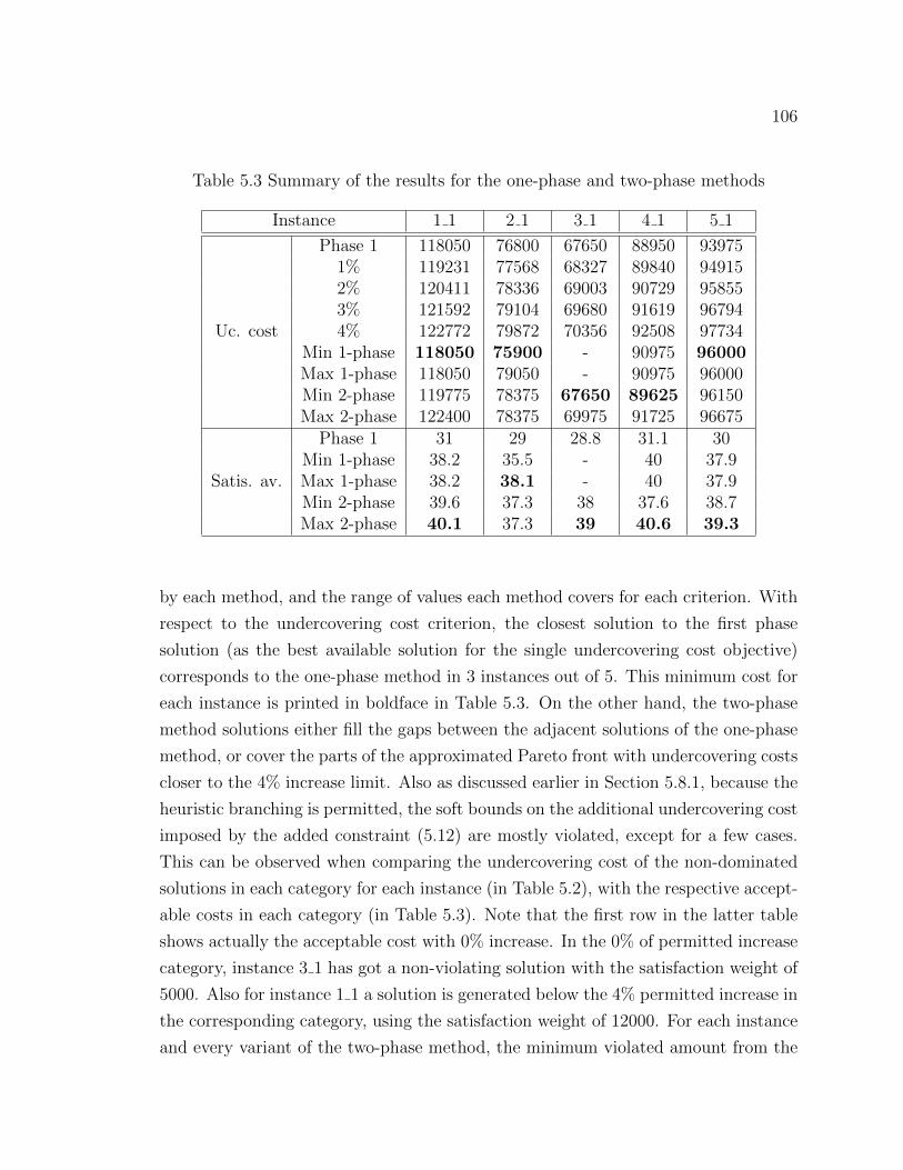
106

Table 5.3 Summary of the results for the one-phase and two-phase methods

Instance 1 1 2 1 3 1 4 1 5 1

Uc. cost

Phase 1 118050 76800 67650 88950 939751% 119231 77568 68327 89840 949152% 120411 78336 69003 90729 958553% 121592 79104 69680 91619 967944% 122772 79872 70356 92508 97734

Min 1-phase 118050 75900 - 90975 96000Max 1-phase 118050 79050 - 90975 96000Min 2-phase 119775 78375 67650 89625 96150Max 2-phase 122400 78375 69975 91725 96675

Satis. av.

Phase 1 31 29 28.8 31.1 30Min 1-phase 38.2 35.5 - 40 37.9Max 1-phase 38.2 38.1 - 40 37.9Min 2-phase 39.6 37.3 38 37.6 38.7Max 2-phase 40.1 37.3 39 40.6 39.3

by each method, and the range of values each method covers for each criterion. With

respect to the undercovering cost criterion, the closest solution to the first phase

solution (as the best available solution for the single undercovering cost objective)

corresponds to the one-phase method in 3 instances out of 5. This minimum cost for

each instance is printed in boldface in Table 5.3. On the other hand, the two-phase

method solutions either fill the gaps between the adjacent solutions of the one-phase

method, or cover the parts of the approximated Pareto front with undercovering costs

closer to the 4% increase limit. Also as discussed earlier in Section 5.8.1, because the

heuristic branching is permitted, the soft bounds on the additional undercovering cost

imposed by the added constraint (5.12) are mostly violated, except for a few cases.

This can be observed when comparing the undercovering cost of the non-dominated

solutions in each category for each instance (in Table 5.2), with the respective accept-

able costs in each category (in Table 5.3). Note that the first row in the latter table

shows actually the acceptable cost with 0% increase. In the 0% of permitted increase

category, instance 3 1 has got a non-violating solution with the satisfaction weight of

5000. Also for instance 1 1 a solution is generated below the 4% permitted increase in

the corresponding category, using the satisfaction weight of 12000. For each instance

and every variant of the two-phase method, the minimum violated amount from the

107

maximum permitted undercovering cost by a non-dominated solution obtained in that

category is calculated. For instances 1 1 to 5 1, the average percentage of minimum

violation in a category with a violating non-dominated solution is calculated as 1.1%,

1%, 1.4%, 0.8% and 2%, respectively. So on average, a bound is violated at least by

1.3% in any violating non-dominated solution.

Also, the minimum average satisfaction rate among the non-dominated solutions

obtained by the two-phase method is compared with the average satsifaction rate of

the solution obtained at the end of the first phase, in each of the instances. This

comparison shows, for each instance, the minimum extent of improvement in the

average satisfaction rate caused by the second phase. The average of the minimum

percentage improvement in the average satisfaction rate caused by the second phase

over 5 instances is 28%. This amount shows the effectiveness of the second phase.

Also, the superiority of the two-phase method over the one-phase method is proved

to be in obtaining non-dominated solutions with higher average satisfaction rate.

Only in instance 2 1, the one-phase method succeeded in finding a solution with

the best average satisfaction rate. The maximum average satisfaction rate for the

non-dominated solutions of each instance is marked in boldface in Table 5.3.

Another conclusion is that the one-phase method is more sensitive to the satisfac-

tion weight changes. No non-dominated solution is generated, for any instance, with

satisfaction weight of 12000 by the one-phase method, which also has an acceptable

undercovering cost below the 4% increase. While the two-phase method is success-

fully generating the acceptable non-dominated solutions by any satisfaction weight.

However, the two-phase method performs less successfully in variants allowing more

than 1% additional undercovering cost. Also varying the satisfaction weights in the

one-phase method results in big jumps in the undercovering cost of the successive

solutions, while in the two-phase method costs are slightly increased between the ad-

jacent solutions resulted by successively increasing the satisfaction weight. That is

why the two-phase method solutions cover the gaps between the one-phase method

solutions on the estimated Pareto-front.

5.8.3 Balancing employee satisfaction rates

In the PBAA problem, there is no seniority ranking defined for employees. There-

fore, apart from maximizing the average satisfaction rate, it might be interesting

to provide a balance in satisfying the employees such that the employees get their

108

preferences all to the same extent, as much as possible. To determine how far the

satisfaction rates are spread out from one another, their distance from their average

value (standard deviation) can be considered as a measure. Therefore, in the two-

phase method it is proposed to control this distance while maximizing the average

satisfaction in the second phase. The RH procedure can help keeping a constant con-

trol along the optimization procedure. At each time slice, the following adaptation is

made to contribute as much as possible to the minimization of the standard deviation

of satisfaction rates.

At each time slice, for each employee e ∈ E, a weight wIne is calculated based on

the employee satisfaction rate distance from the average satisfaction rate of employees

in the partial solution before the current time slice. This average value is denoted by

RInAve. In the objective function, the satisfaction rate of each employee is multiplied by

his/her corresponding weight. If the overlap between time slices is denoted by ov, then

the previous time slice ends at period p1 +ov−1. We have RInAve =

∑e∈E

Rp1+ov−1e

|E| , where

Rp1+ov−1e is calculated for segments Sp1+ov−1

e after removing the activity assignments

in the overlap between the current time slice and the previous one. To calculate the

employees weight factors, let 0 ≤ wmin ≤ 1 and wmax ≥ 1 be parameters, indicating

respectively the minimum and maximum values for wIne for all employees e ∈ E.

In our tests, these parameters are respectively set equal to 0.5 and 2. Then wIne is

calculated as:

wIne =

1 + (wmax − 1)RIn

Ave−Rp1+ov−1e

RInAve

if Rp1+ov−1e < RIn

Ave

1− (1− wmin)R

p1+ov−1e −RIn

Ave

1−RInAve

otherwise(5.27)

By this method, weights greater/smaller than 1 represent the employees with sat-

isfaction levels less/more than average, giving a higher/lower priority to increase their

satisfaction rates in the current time slice. So the employees with lower satisfaction

rates, so far, are going to become more satisfied by the current time slice activity

assignment. By the definition given in (5.27), this weight for an employee with 0

satisfaction so far takes the maximum value wmax, while it takes the minimum value

wmin if the employee is completely satisfied (with satisfaction rate Rp1+ov−1e = 1). If

employee e has no low or high-preference qualification or Sp1+ov−1e is empty, we do not

incorporate the satisfaction rate of employee e in the average value calculation. For

these employees we set the weight wIne = 1. For the first time slice, we set wIne = 1,

109

for all employees.

According to the above strategy, another series of experiments is conducted to eval-

uate the effects of such adjustments to the second phase of the two-phase method, on

the employee satisfaction rates standard deviation, as well as on the average satisfac-

tion rate obtained. Two variants are considered here for the two-phase method, one

with updates of employee weights in each time slice and the other which considers no

weight updates for employees. For the second variant we refer to the results reported

in Section 5.8.2. The standard deviation of satisfaction rates is calculated for each

instance and each run with different values for parameters ε and w22. The 5 instances

are also solved with the first variant in several runs for the same value of parameters

ε and w22. The RH procedure is applied for the second phase with slice length 720, as

well as the branching strategy selected based on the settings resulted in Section 5.8.1.

In Table 5.4, the average value over the 5 instances, for the average satisfaction rates

and standard deviation values are presented for all the combinations of the ε and

w22 parameters, separately for the two variants. The same average values are also

reported for the one-phase method results over the 5 instances (as presented again in

Section 5.8.2). Finally, the efficiency of the two-phase method variant with employee

weight updating is compared with the other variant with no weight updates, as well

as the one-phase method.

Table 5.4 Results for considering employee weight updates along the time slices

Var AtrTwo-phase

ε=0 ε=1 ε=23000 5000 9000 12000 3000 5000 9000 12000 3000 5000 9000 12000

NWAv 37.5 38.1 38.9 39.6 37.7 38.7 39.4 39.5 37.9 38.5 39.6 39.6Std 12 12 12 12 11.9 12.3 12.2 11.8 12 12.1 12.2 12

WAv 37.7 38.3 39.3 39.7 37.8 38.5 39.3 39.7 37.8 38.7 39.2 39.7Std 11.3 11.3 11.2 11.2 11.3 11.1 11.1 11 11 11.3 11 10.9

Two-phaseOne-phase

ε=3 ε=43000 5000 9000 12000 3000 5000 9000 12000 3000 5000 9000 12000

NWAv 38.2 38.8 39.5 39.6 38.5 38.7 39.8 40.1 37.5 38.7 40 41.1Std 11.8 12 11.7 12.1 12 12.1 12 12.3 12.2 11.9 12.3 12.2

WAv 38.1 39 39.5 39.9 38.4 39.1 39.5 39.9Std 11.1 11.3 11.2 11.3 11.4 11.6 11.2 11.2

110

In Table 5.4, the first column specifies the two variants respectively denoted by

NW (no weight updating) and W (weight updating). The second column introduces

the type of information the average values reported in each row of the table correspond

to, which is either the average (Av.) or the standard deviation (Std) of the satisfaction

rates. The rest of columns give the results, first for the two-phase method, and then

for the one-phase method.

First, we compare the data corresponding to the solutions of the two-phase method,

in the variant with employee weights updating, and the variant which does not con-

sider weight updates for employees. It can be seen that the maximum value of satis-

faction rates standard deviation observed among the solutions of the former variant

(11.6) is less than the minimum value of this measure in the latter variant (11.7).

With respect to the average satisfaction rates, average values over the instances does

not vary much for the two variants. The one-phase method, on average, obtains so-

lutions with higher standard deviation (with value of 12.1) and average satisfaction

rate (with value of 39.3), compared to both variants of the two-phase method. This

comparison between the two variants of the two-phase method shows an increase in

the standard deviation (from 11.2 to 12) and a small decrease in average satisfaction

rate (from 39 to 38.9) from the former variant to the latter. So, on average, using the

proposed strategy to update the employees weights during the RH procedure seems to

be successful in finding the solutions in which employees satisfaction rates are slightly

more balanced.

Now we want to see what happens if we also consider the dominance properties

between the solutions of each instance. The average of the two measures above

are calculated only over the non-dominated solutions in each of the instances, and

separately for these solutions obtained by the one-phase and two-phase methods. The

average of the resulted values over all the instances are reported as 38.2 and 12.7, for

the one-phase method non-dominated solutions compared to the two-phase method

solutions with no employee weight updating. For the two-phase method solutions with

no employee weight updating, these values are respectively equal to 38.7 and 12. On

the other hand, these values are equal to 38.8 and 11.7, respectively, for the one-phase

method non-dominated solutions compared to the two-phase method solutions with

employee weight updating. Finally, these values for the two-phase method solutions

with employee weight updating are respectively equal to 38.6 and 11.2. So, applying

the employee weight updating strategy is proved to be more efficient compared to the

111

one-phase method and the other two-phase variant with no employee weight updates,

in gaining the balance among employee satisfaction rates.

5.8.4 A unique undercovering cost

We also conduct the tests on slightly modified 5 instances generated primarily,

in which the same undercovering cost cUca = 100 is defined for all activities a ∈A. All the other attributes of these instances stay the same as what explained in

Section 5.7. These new instances are numbered from 1 2 to 5 2. Both one-phase and

two-phase methods are applied on these instances for the same executions described

in Section 5.8.2. For the second phase of the two-phase method, the same RH and

branching parameters are used. In addition to that, we apply the employee weight

updating procedure along the time slices. In Table 5.5, we report the average values

for the results obtained and compare them with the same type of results for the

instances with unmodified varying undercovering costs. We denote the former and

latter set of instances respectively by Unq and Var. The reported information include

the undercovering percentage (to be able to compare both sets of instances together),

average satisfaction rate and the solution time. The purpose is to see if selecting the

undercovering costs that vary from one activity to the other makes any privilege for

the two-phase method over the one-phase method.

Based on the information of Table 5.5, considering the varying undercovering

costs for different activities generally results in obtaining the solutions with lower

percentage of undercovering and average satisfaction rates, no matter which solution

method (one-phase or two-phase) is used. Considering the solution times, the results

are again better with this variant. This improvement in solution times can be observed

especially in the two-phase method when allowing higher percentage of increase in the

undercovering cost. If the same data processing considering the dominance properties

of solutions (as described in Section 5.8.3 to calculate the average values only by

considering the non-dominated solutions) is applied here, this conclusion is still valid,

with the average values reported in Table 5.6 for both instance groups.

In Table 5.6, the percentage of undercovering, average satisfaction rate and solu-

tion time values are reported for each of the one-phase and two-phase methods on

average over 5 instances of each group. With the varying undercovering costs, the

average percentage of the two-phase method solutions which are non-dominated (with

value of 11%) is higher than this average for the instances with a unique cost (with

112

Table 5.5 Results on instances with varying and unique undercovering cost for activ-ities

Var AtrOne-phase

Two-phase0 1

3000 5000 9000 12000 3000 5000 9000 12000 3000 5000 9000 12000

UnqUc% 1.4 1.4 1.4 1.4 1.4 1.4 1.4 1.4 1.4 1.4 1.4 1.5

Av 38.5 39.2 40.3 40.7 38.9 39.2 39.9 40.2 39.2 39.7 40.0 40.4time 129 142 154 165 246 251 245 263 220 211 217 214

VarUc% 1.2 1.2 1.2 1.3 1.2 1.2 1.2 1.2 1.2 1.2 1.2 1.2

Av 37.5 38.7 40 41.1 37.7 38.3 39.3 39.7 37.8 38.5 39.3 39.7time 115 110 111 109 215 212 208 205 239 232 228 215

Two-phase2 3 4

3000 5000 9000 12000 3000 5000 9000 12000 3000 5000 9000 12000

UnqUc% 1.5 1.5 1.5 1.5 1.5 1.5 1.5 1.5 1.5 1.5 1.5 1.5

Av 39.1 39.9 40.2 40.4 39.4 40.1 40.5 40.6 39.3 39.9 40.6 40.7time 382 402 440 408 423 424 387 369 416 422 415 418

VarUc% 1.2 1.2 1.2 1.2 1.2 1.2 1.2 1.3 1.2 1.3 1.2 1.3

Av 37.8 38.7 39.2 39.7 38.1 39 39.5 39.9 38.4 39.1 39.5 39.9time 255 245 247 224 266 271 235 226 266 246 258 236

Table 5.6 Average results for the instances with varying and unique undercoveringcost

Inst.group

Attribute One-phase Two-phase

UnqUc% 1.4 1.4

Satis. Av. 39.7 40Time 149 320

VarUc% 1.2 1.2

Satis. Av. 38.4 38.6Time 120 217

113

value of 7%). This percentage is lower for the one-phase method in the instances

with varying undercovering cost (with value of 40%) compared to the ones with a

unique undercovering cost (with value of 45%). Besides, the one-phase method is

sensitive to the satisfaction weights when applied to solve the instances with varying

undercovering cost, more than when used to solve the instances with unique under-

covering cost. This can be observed from the number of non-dominated solutions

obtained with the higher weights, such that except for one instance, in all instances

only one non-dominated solution is found and that is either with weight 3000 or 5000.

The reason is that if a non-dominated solution is found with other weights with the

one-phase method, its undercovering cost is far beyond the acceptable 4% additional

cost. Contrarily, the two-phase method is more sensitive to satisfaction weights when

solving the instances with unique undercovering cost. In this case, the non-dominated

solutions are all obtained with the satisfaction weights 9000 and 12000. So in gen-

eral, the two-phase method is working more efficiently when solving the instances

with varying undercovering cost for activities, than the instances with a unique un-

dercovering cost for all activities. However the one-phase method works better for

the unique cost than for the varying costs.

5.8.5 Arc elimination

Five different procedures to eliminate arcs are compared together in this part.

These procedures are applied based on the exact and heuristic methods proposed in

Section 5.6. This series of experiments are applied on the modified instances with

unique undercovering cost for activities. Since this modification in undercovering

costs proved to result in higher solution times, we used these instances to be able to

better evaluate the time savings by applying the arc elimination procedures. On the

other hand, only the heuristic column-fixing branching is used to solve both phases

of the two-phase method. In fact the selection of the branching method and the

quality of the second phase solution has no impact on the number of arcs eliminated.

The percentage of the arcs eliminated depends only on the solution obtained in the

first phase. The second phase solution at a given time slice does not influence the

percentage of arcs to be removed in the next time slice. So partial solutions obtained

in the second phase as well as the method used to obtain them do not have an

impact on the arc elimination procedure. The only impact would be the quality of

the solution obtained in the first phase.

114

The procedure to remove the arcs takes some computational time, by itself. So

the result of arc elimination should have enough impact in further reducing the com-

putational time by network reductions, in order to be worthwhile in general. Using

the heuristic branching and solving both phases in several time slices helps avoiding

extra solution times. So, here we want to evaluate if any arc elimination procedure

is able to reduce the solution time significantly.

In Table 5.7, six attributes are monitored for every instance solved by different arc

elimination procedures, compared also with the case in which no arc elimination pro-

cedure is applied. These attributes, in successive order, are the number of transitions,

the number of undercoverings, average satisfaction rate, solution time, percentage of

the second phase solution time and percentage of the arcs eliminated. The heuristic

methods in Section 5.6 are denoted in this table respectively by H1, H2 and H3. For

the third heuristic method two variants are tested: one which keeps only the high-

preference activity assignments from the first phase solution (denoted by H3(h)), and

the other which keeps both high and low preference activity assignments (denoted by

H3(h+ l)).

From the results we make the following observations. The number of undercov-

erings after applying any of the arc elimination procedures is almost the same as

the original procedure with no arc elimination. So, it shows that all the procedures

are successful in keeping the quality of the first phase solution with respect to the

number of undercoverings. On the other hand, the exact arc elimination procedure

also keeps the same quality with respect to the average satisfaction rate, as expected,

with more or less the same solution times. However, arc elimination fails to keep

the quality of the solution with respect to the average satisfaction rate, the most by

the first two heuristic procedures. The first heuristic procedure is the worst, since it

removes the largest number of arcs. Although, in these cases the solution times drop

a little below the exact solution times. By the third heuristic procedure variants, the

more satisfactory would be the average satisfaction rates obtained, the more highly

preferred activity assignments (and less lowly preferred ones) are kept from the first

phase solution. However the results are still lower in quality than the exact solutions,

while the solution time reaches almost the same amount. This trend can also be seen

by analyzing the last two attributes. The percentage of the solution time spent in the

second phase reduces in the first two heuristic procedures, and grows again around

the original percentage, by the third and fourth procedures. The reason can be seen

115

Table 5.7 Results of the two-phase method variants

Instance AttributeNoarc

Arc elimination variants

elim Exact H1 H2 H3(h) H3(h+l)

1 2

Trns 564 564 595 589 574 583# Uc 88 88 88 88 88 88S av. 40.3 40.3 31.8 32.8 38.5 37.5Time 84 84 79 73 85 87

% phase2 T 29 29 14 15 21 18% arc elim 0.1 25 25 5 8

2 2

Trns 571 573 602 607 582 584# Uc 59 59 59 59 58 58S av. 37.2 37.2 29.2 31 35.6 34.5Time 89 95 73 72 97 99

% phase2 T 26 26 13 12 28 24% arc elim 1.5 26 25 5 8

3 2

Trns 543 439 565 560 556 561# Uc 55 55 55 55 54 54S av. 39.2 39 30.3 32 37 35.2Time 81 91 82 75 90 87

% phase2 T 25 34 10 13 30 33% arc elim 2.7 26 25 6 9

4 2

Trns 583 583 615 612 593 592# Uc 84 84 84 84 85 85S av. 40.8 40.8 32.9 34.9 39.9 39.1Time 102 108 86 86 108 103

% phase2 T 28 33 11 11 31 26% arc elim 0.2 26 25 5 9

5 2

Trns 581 581 603 586 592 597# Uc 79 79 79 79 79 79S av. 39.5 39.5 31 34.4 38 36.4Time 90 94 77 71 91 86

% phase2 T 22 25 11 13 28 21% arc elim 1.3 25 24 5 10

116

in the percentage of arcs eliminated in the last row for each instance. This shows

that even by the best heuristic procedure (the column before the last), almost the

same amount of time as the exact procedure is finally spent in the second phase. The

useful arcs in keeping the quality of the solution need to be detected by procedures

whose application spent back the time saved by the elimination of a small percentage

of arcs. As a conclusion none of the arc elimination procedures proved to be efficient.

5.9 CONCLUSION

In this chapter, we look for a tool to obtain solutions for the activity assignment

problem to work shifts, which in the first place, incur the minimum undercovering

cost, and in the second place, provide the maximum employee satisfaction with respect

to their individual preferences on doing activities. Because of the multi-objective

nature of the problem and the dominance properties of the solutions studied in this

context, solutions which are violating the minimum cost by a small percentage but

include the more satisfactory assignments for employees are also interesting. This

tool needs to be flexible to efficiently interpret the preferences of the decision makers

on the two objectives in practice, to give a set of non-dominated solutions within the

acceptable range for each objective. Two heuristic methods based on the weighted

sum method (with weights determining the importance of each objective), and the

elastic-constraint method (with an added constraint controlling the degree of violation

of the first objective minimum value) are proposed here. These methods rely on CG

models and are solved with a heuristic RH procedure.

To assess the desired properties for the two proposed methods, a set of experiments

are designed. We performed several runs of the one-phase method with different ob-

jective weight combinations, and several runs of the two-phase method with different

permitted percentage of increase in the minimum undercovering cost and the same set

of weight combinations as the one-phase method. From the results it is concluded that

for a solution obtained by the two-phase method there is a 24% chance of being a non-

dominated solution, and a 5% chance of being dominated only by a one-phase method

solution. While a one-phase solution has a 65% chance of being non-dominated, and

a 30% chance of being dominated only by a two-phase solution. With respect to the

maximum permitted increase in the minimum undercovering cost (by 4%), there is

a higher chance of having an acceptable non-dominated solution by considering 0%

117

and 1% increase in the added constraint. Also setting the satisfaction weight at 3000

brings less chance of having a non-dominated solution, and in case of being domi-

nated, the solution is among the furthest to a non-dominated solution, compared to

the dominated solutions by the other satisfaction weights. The one-phase method,

on the other hand, gets the solutions with big jumps from one satisfaction weight to

the other, and can not be easily under control. So by testing the two-phase variants

considering 0% and 1% undercovering cost increases and satisfaction weights other

than 3000, we can get relatively good solutions with higher average satisfaction rates

in return for acceptable undercovering cost increase. Although the solution times are

higher with the two-phase method and the arc elimination procedures did not succeed

in reducing them, this method can be applied more efficiently in practice. Besides,

when the undercovering costs vary from one activity to the other, this method proves

to perform better. The one-phase method, though, works better for a unique un-

dercovering cost case than the varying costs case, with respect to both the number

of non-dominated solutions obtained, and the sensitivity to the satisfaction weights.

Finally if we want to have equity among employees, the two-phase method can get

the solutions with satisfaction rates less spread out or dispersed from the average

rate, by satisfying the employees with inverse relationship to their satisfaction so far,

in each time slice of the RH procedure. While, in the one-phase method solutions,

the standard deviation of the employee satisfaction rates is generally higher. The em-

ployee weight updating possibility of the two-phase method can also help providing

the equity in the satisfaction rates from one week to the next. At the first time slice

of the next week activity assignment problem, for all employees the weights can be

defined based on the distance their total satisfaction had with the average value at

the end of the previous week.

118

CHAPTER 6

CONCLUSION

6.1 GENERAL DISCUSSION AND CONTRIBUTIONS

To our knowledge, this work is the first to tackle an activity and task assignment

problem that considers different scheduling flexibilities (meal break repositionings,

overtime and temporary workers) to face demand changes a few days prior to the

operations in a service company.

In the first place, a column generation heuristic embedded into a rolling horizon

procedure is proposed to solve the activity assignment problem, with the possibility

of extending the planned work shifts and moving their meal breaks. Computational

results obtained on randomly generated instances in two small-sized and one medium-

sized classes show a reduction in the number of undercoverings on average by 68%,

96%, and 70% in respective classes, compared to the case with no flexibility. The

problem with the solutions is that the computational times are rather high when

considering the flexibilities.

In the second step, we developed an efficient two-phase heuristic. To overcome

the problem complexity, this solution approach uses an approximate mixed-integer

programming model in the first phase to reduce the search space. Given preassigned

tasks, potential temporary shifts and potential overtime periods for regular shifts,

all suggested by the first phase solution, the second phase computes a final solu-

tion using a column generation heuristic embedded into a rolling horizon procedure.

This heuristic was tested on randomly generated medium- to large-sized instances

to compare different variants of flexibility. The computational results show that the

additional flexibilities can yield substantial savings in the number of activity demand

undercoverings and that the solutions can be computed in reasonable computational

times.

Another extension to the activity assignment problem to work shifts, never studied

before, is made in the third step. We tried to study the simultaneous satisfaction of

two objectives: minimizing the undercovering costs, as the most important part of

the costs in such a problem for companies, and providing the satisfaction of employees

119

who are assigned to do these activities. But this is not always easy to have it both

ways, when it comes to these two objectives. The activity assignments which provide

the highest coverage are not neccessarily the ones which satisfy all the employees.

That is why in the multi-objective optimization context, we have ”Pareto-optimal”

solutions rather than ”optimal” solutions. We suppose that the former objective still

has more importance over the latter one. But decision makers may still be willing

to have a small percentage of increase in the undercovering cost by an assignment,

if by another assignment incurring that higher cost more satisfaction can be brought

to any employee(s). Two models and solution methods are proposed in this chapter

to solve this problem. In one method we need to give an importance weight to each

objective and optimize the weighted sum of the objective values. In the other one, we

first find the optimized value for the more important objective and then optimize the

value of the other objective by not letting the value of the first objective to increase

by more than a desired percentage. Both methods rely on column generation models

solved with a heuristic rolling horizon procedure.

The second method outperforms the weigthing method which transforms the prob-

lem to a single-objective one with weighted sum of different objectives, in terms of

practicality. On the one hand, it doesn’t have the weighting method difficulty in

setting weights. On the other hand it gives the decision maker more control over

finding the solutions with undercoverings slightly above the minimum, in favor of

better satisfying employees preferences. This method also has more capacity in pro-

viding a set of non-dominated solutions within the desired range of objective values.

In addition, it provides a flexible tool for decision makers, to be able to select the best

solution which fits their varying needs, while it is easy to interpret their preferences

over the objectives. Besides, when the undercovering costs vary from one activity to

the other, this method proves to perform better. By adapting the two-phase method

to update the weights for each employee from one slice to the other, the satisfaction

of employees can be balanaced throughout the horizon. However the computational

times are higher with the two-phase method, and the attempts to reduce them failed

to make a difference.

Hence, this research provides the service industries with an efficient tool to deal

with the last-minute changes in demands using different flexibilities in the personnel

scheduling process, leading to cost and time savings. On the other hand, it introduces

a guideline to companies to incorporate as much as possible the employees preferences

120

in setting satisfactory work schedules while keeping the costs at minimum levels.

6.2 FUTURE WORK

This thesis referred to some extensions of the activity/task assignment problem

to work shifts. Other extensions can also be studied, examples of which are cited as

follows.

As a future work on the ATTFF problem in Chapter 4, extending the first-phase

model can be considered in order to include also the break movements, bounds on

segment durations and transition costs. By further extensions we may be able to

reduce the computational times by possibly avoiding the column generation heuristic

process in the second phase. Additionally, we can consider other real-world rules

such as maximum working time over a week for each employee. This rule affects the

decision on regular shift extensions. Finding a way to deal with the soft constraints on

the minimum working time over a week for each employee, or on activity assignment

durations can also be tackled.

As another example, for the PBAA problem in Chapter 5, the proposed two-phase

method can be applied in a single solution process to obtain a set of non-dominated

solutions in less computational time. The first phase problem can only be solved

once, while the obtained minimum undercovering cost is recorded to be used in the

right-hand side value of the added constraint in the consecutive runs of the second

phase problem with varying value for ε and the satisfaction weight.

In the problems studied in this thesis, it is assumed that scheduling is performed

just a few days before the operations. Real-time optimization tools also need to

be provided during the operations, to deal with changes in demands, availability

of personnel or their preferences. This area corresponds to a field of research that

remains unexplored at the moment.

121

REFERENCES

ACHOUR, H., GAMACHE, M., SOUMIS, F. and DESAULNIERS, G. (2007). An

exact solution approach for the preferential bidding system problem in the airline

industry. Transportation Science, 41, 354–365.

ADDOU, I. and SOUMIS, F. (2007). Bechtold-jacobs generalized model for shift

scheduling with extraordinary overlap. Annals of Operations Research, 155, 177–

205.

AICKELIN, U. and DOWSLAND, K. A. (2004). An indirect genetic algorithm for

a nurse-scheduling problem. Computers and Operations Research, 31, 761–778.

AYKIN, T. (1996). Optimal shift scheduling with multiple break windows. Man-

agement Science, 42, 591–602.

BARD, J. F., BINICI, C. and DESILVA, A. H. (2003). Staff scheduling at the United

States Postal Service. Computers & Operations Research, 30, 745–771.

BARD, J. F., MORTON, D. P. and WANG, Y. M. (2007). Workforce planning at

USPS mail processing and distribution centers using stochastic optimization. Annals

of Operations Research, 51–78.

BARD, J. F. and PURNOMO, H. W. (2005). Preference scheduling for nurses using

column generation. European Journal of Operational Research, 164, 510–534.

BARD, J. F. and WAN, L. (2005). Weekly scheduling in the service industry: an

application to mail processing and distribution centers. IIE Transactions, 37, 379–

396.

BARD, J. F. and WAN, L. (2006). The task assignment problem for unrestricted

movement between workstation groups. Journal of Scheduling, 9, 315–341.

BARD, J. F. and WAN, L. (2008). Workforce design with movement restrictions

between workstation groups. Manufacturing & Service Operations Management, 10,

24–42.

BARNHART, C., JOHNSON, E., NEMHAUSER, G., SAVELSBERGH, M. and

VANCE, P. (1998). Branch-and-price: column generation for solving huge integer

programs. Operations Research, 46, 316–329.

122

BECHTOLD, S. E. and JACOBS, L. E. (1990). Implicit modeling of flexible break

assignments in optimal shift scheduling. Management Science, 36, 1339–1351.

BEDDOE, G. R. and PETROVIC, S. (2006). Selecting and weighting features

using a genetic algorithm in a case-based reasoning approach to personnel rostering.

European Journal of Operational Research, 175, 649–671.

BELLANTI, F., CARELLO, G., CROCE, F. D. and TADEI, R. (2004). A greedy-

based neighborhood search approach to a nurse rostering problem. European Journal

of Operational Research, 153, 28–40.

BOUBAKER, K., DESAULNIERS, G. and ELHALLAOUI, I. (2010). Bidline

scheduling with equity by heuristic dynamic constraint aggregation. Transporta-

tion Research Part B: Methodological, 44, 50–61.

BOUCHARD, M. (2004). Optimisation des pauses dans le probleme de fabrication

d’horaires avec quarts de travail. Master’s thesis, Ecole Polytechnique, Montreal,

Canada.

BURKE, E. K., CURTOIS, T., POST, G., QU, R. and VELTMAN, B. (2008). A

hybrid heuristic ordering and variable neighbourhood search for the nurse rostering

problem. European Journal of Operational Research, 188, 330–341.

BURKE, E. K., DE CAUSMAECKER, P., BERGHE, G. V. and VAN LAN-

DEGHEM, H. (2004). The state of the art of nurse rostering. Journal of Scheduling,

7, 441–499.

CHANKONG, V. and HAIMES, Y. Y. (1983). Multiobjective Decision Making The-

ory and Methodology. Elsevier Science, New York.

CHU, S. C. (2007). Generating, scheduling and rostering of shift crew-duties: Ap-

plications at the hong kong international airport. European Journal of Operational

Research, 177, 1764–1778.

COTE, M.-C., GENDRON, B., QUIMPER, C.-G. and ROUSSEAU, L.-M. (2011a).

Formal languages for integer programming modeling of shift scheduling problems.

Constraints, 16, 54–76.

COTE, M.-C., GENDRON, B. and ROUSSEAU, L.-M. (2011b). Grammar-based

integer programming models for multiactivity shift scheduling. Management Science,

57, 151–163.

123

COTE, M.-C., GENDRON, B. and ROUSSEAU, L.-M. (2012). Grammar-based col-

umn generation for personalized multi-activity shift scheduling. INFORMS Journal

on Computing, In Press.

DANTZIG, G. B. (1954). A comment on Edie’s “traffic delays at toll booths”.

Operations Research, 2, 339–341.

DEMASSEY, S., PESANT, G. and ROUSSEAU, L.-M. (2005). Constraint program-

ming based column generation for employee timetabling. R. Bartak and M. Milano,

editeurs, Integration of AI and OR Techniques in Constraint Programming for Com-

binatorial Optimization Problems, Springer Berlin / Heidelberg, vol. 3524 de Lecture

Notes in Computer Science. 830–833.

DESAULNIERS, G., DESROSIERS, J. and SOLOMON, M. (2005). Column Gen-

eration. Cahiers du GERAD. Springer, New York, NY.

DORNBERGER, R., FREY, L. and HANNE, T. (2008). Single and multiobjective

optimization of the train staff planning problem using genetic algorithms. IEEE

Congress on Evolutionary Computation. Hong Kong, China, June 1-6, 970–977.

DOWSLAND, K. A. (1998). Nurse scheduling with tabu search and strategic oscil-

lation. European Journal of Operational Research, 106, 393–407.

EASTON, F. and MANSOUR, N. (1999). A distributed genetic algorithm for deter-

ministic and stochastic labor scheduling problems. European Journal of Operational

Research, 118, 505–523.

EHRGOTT, M. and GANDIBLEUX, X. (2000). A survey and annotated bibliogra-

phy of multiobjective combinatorial optimization. OR Spectrum, 22, 425–460.

EHRGOTT, M. and RYAN, D. M. (2002). Constructing robust crew schedules with

bicriteria optimization. Journal of Multi-Criteria Decision Analysis, 11, 139–150.

ERNST, A., JIANG, H., KRISHNAMOORTHY, M., OWENS, B. and SIER, D.

(2004a). An annotated bibliography of personnel scheduling and rostering. Annals

of Operations Research, 127, 21–144.

ERNST, A. T., JIANG, H., KRISHNAMOORTHY, M. and SIER, D. (2004b). Staff

scheduling and rostering: A review of applications, methods and models. European

Journal of Operational Research, 153, 3–27.

GAMACHE, M., SOUMIS, F., VILLENEUVE, D., DESROSIERS, J. and

GELINAS, E. (1998). The Preferential Bidding System at Air Canada. Trans-

portation Science, 32, 246–255.

124

HANNE, T., DORNBERGER, R. and FREY, L. (2009). Multiobjective and

preference-based decision support for rail crew rostering. IEEE Congress on Evolu-

tionary Computation. Trondheim Norway, May 18-21, 990–996.

HANSEN, J. and LIDEN, T. (2005). Group construction for airline cabin crew:

Comparing constraint programming with branch and price. R. Bartak and M. Mi-

lano, editeurs, Integration of AI and OR Techniques in Constraint Programming for

Combinatorial Optimization Problems, Springer Berlin / Heidelberg, vol. 3524 de

Lecture Notes in Computer Science. 928–930.

HUR, D., MABERT, V. A. and BRETTHAUER, K. M. (2004). Real-time schedule

adjustment decisions: a case study. Omega, 32, 333–344.

JIN, J. (2009). Pre-affectation des taches aux employees effectuant des taches non-

interruptibles et des activites interruptibles. Master’s thesis, Ecole Polytechnique,

Montreal, Canada.

LEQUY, Q., BOUCHARD, M., DESAULNIERS, G., SOUMIS, F. and TACHE-

FINE, B. (2012a). Assigning multiple activities to work shifts. Journal of Scheduling,

15, 239–251.

LEQUY, Q., DESAULNIERS, G. and SOLOMON, M. (2010). Assigning Team Tasks

and Multiple Activities to Fixed Work Shifts. Les Cahiers du GERAD G-2010-71.

Groupe d’etudes et de recherche en analyse des decisions (Montreal, Quebec).

LEQUY, Q., DESAULNIERS, G. and SOLOMON, M. M. (2012b). A two-stage

heuristic for multi-activity and task assignment to work shifts. Computers & Indus-

trial Engineering, In Press.

LOUCKS, J. S. and JACOBS, F. R. (1991). Tour scheduling and task assignment of

a heterogeneous work force: A heuristic approach. Decision Sciences, 22, 719–738.

LUBBECKE, M. and DESROSIERS, J. (2005). Selected topics in column genera-

tion. Operations Research, 53, 1007–1023.

MAENHOUT, B. and VANHOUCKE, M. (2010). A hybrid scatter search heuristic

for personalized crew rostering in the airline industry. European Journal of Opera-

tional Research, 206, 155–167.

MARLER, R. T. and ARORA, J. S. (2004). Survey of multi-objective optimization

methods for engineering. Structural and Multidisciplinary Optimization, 26, 369–395.

125

MOUDANI, W. E., COSENZA, C. A. N., DE COLIGNY, M. and MORA-CAMINO,

F. (2001). A bi-criterion approach for the airlines crew rostering problem. Evolution-

ary Multi-Criterion Optimization: First International Conference. Zurich, Switzer-

land, March 7-9, 486–500.

MOZ, M. and PATO, M. V. (2007). A genetic algorithm approach to a nurse reros-

tering problem. Computers & Operations Research, 34, 667–691.

OMARI, Z. (2002). Attribution des activites aux employes travaillant sur des quarts.

Master’s thesis, Ecole Polytechnique, Montreal, Canada.

OZKARAHAN, I. (2000). Allocation of surgeries to operating rooms by goal pro-

graming. Journal of Medical Systems, 24, 339–378.

REKIK, M., CORDEAU, J.-F. and SOUMIS, F. (2004). Using benders decom-

position to implicitly model tour scheduling. Annals of Operations Research, 128,

111–133.

REKIK, M., CORDEAU, J.-F. and SOUMIS, F. (2008). Solution approaches to

large shift scheduling problems. RAIRO-Operations Research, 42, 229–258.

REKIK, M., CORDEAU, J.-F. and SOUMIS, F. (2010). Implicit shift scheduling

with multiple breaks and work stretch duration restrictions. Journal of Scheduling,

13, 49–75.

TOPALOGLU, S. and OZKARAHAN, I. (2003). Implicit optimal tour scheduling

with flexible break assignments. Computers and Industrial Engineering, 44, 75–89.

VALOUXIS, C. and HOUSOS, E. (2000). Hybrid optimization techniques for

the workshift and rest assignment of nursing personnel. Artificial Intelligence in

Medicine, 20, 155–175.

VATRI, E. (2001). Integration de la generation de quarts de travail et de l’attribution

d’activites. Master’s thesis, Ecole Polytechnique, Montreal, Canada.

WONG, G. and CHUN, A. H. W. (2004). Constraint-based rostering using meta-

level reasoning and probability-based ordering. Engineering Applications of Artificial

Intelligence, 17, 599–610.

YEH, J.-Y. and LIN, W.-S. (2007). Using simulation technique and genetic algorithm

to improve the quality care of a hospital emergency department. Expert Systems with

Applications, 32, 1073–1083.

126

ZADEH, L. A. (1963). Optimality and Non-Scalar-Valued Performance Criteria.

IEEE Transactions on Automatic Control, 8, 59–60.

ZHANG, X., CHAKRAVARTHY, A. and GU, Q. (2009). Equipment scheduling

problem under disruptions in mail processing and distribution centres. Journal of

the Operational Research Society, 60, 598–610.