Dbt Thesis Ucla
116
University of Calif ornia Los Angeles Microstructural Effect on the Ductile-to-Brittle Transition in Body Centered Cubic Metals Investigation by Three Dimensional Dislocation Dynamics Simulations A dissertation submitted in partial satisfaction of the requirements for the degree Doctor of Philosophy in Mechanic al and Aerospace Engineering by Jianming Huang 2004
Transcript of Dbt Thesis Ucla
8/8/2019 Dbt Thesis Ucla
http://slidepdf.com/reader/full/dbt-thesis-ucla 1/116
University of California
Los Angeles
Microstructural Effect on the Ductile-to-Brittle
Transition in Body Centered Cubic Metals
Investigation by Three Dimensional Dislocation
Dynamics Simulations
A dissertation submitted in partial satisfaction
of the requirements for the degree
Doctor of Philosophy in Mechanical and Aerospace Engineering
by
Jianming Huang
2004

8/8/2019 Dbt Thesis Ucla
http://slidepdf.com/reader/full/dbt-thesis-ucla 2/116
c
Copyright by
Jianming Huang
2004

8/8/2019 Dbt Thesis Ucla
http://slidepdf.com/reader/full/dbt-thesis-ucla 3/116
The dissertation of Jianming Huang is approved.
Vijay Gupta
H. Thomas Hahn
Jiann-Wen (Woody) Ju
Nasr M. Ghoniem, Committee Chair
University of California, Los Angeles
2004
ii
8/8/2019 Dbt Thesis Ucla
http://slidepdf.com/reader/full/dbt-thesis-ucla 4/116
To my wife Cynthia . . .
for her support, love, encouragement, and understanding
during the completion of this thesis
iii
8/8/2019 Dbt Thesis Ucla
http://slidepdf.com/reader/full/dbt-thesis-ucla 5/116

8/8/2019 Dbt Thesis Ucla
http://slidepdf.com/reader/full/dbt-thesis-ucla 6/116
4.6 Interaction with SIA cluster atmosphere . . . . . . . . . . . . . . 40
4.7 Formation of PSBs . . . . . . . . . . . . . . . . . . . . . . . . . . 43
4.8 PDD in Nonlinear Equation . . . . . . . . . . . . . . . . . . . . . 47
5 Three Dimensional Crack Simulation with Discrete Dislocation
Representation Method . . . . . . . . . . . . . . . . . . . . . . . . . . 49
5.1 Discrete Model in 3D cracks . . . . . . . . . . . . . . . . . . . . . 50
5.2 Numerical Simulation of General 3-D Crack . . . . . . . . . . . . 54
5.2.1 Penny-shaped crack . . . . . . . . . . . . . . . . . . . . . . 54
5.2.2 Effect of Non-uniform Stress . . . . . . . . . . . . . . . . . 59
5.2.3 2-D straight crack . . . . . . . . . . . . . . . . . . . . . . . 61
6 Dislocation Activity ahead of Crack Tip . . . . . . . . . . . . . . 66
6.1 Three Dimensional Elastic Dislocation Interaction with the Crack 66
6.2 Motion of Dislocation ahead of Crack Tip . . . . . . . . . . . . . 70
6.3 Dislocation Nucleation . . . . . . . . . . . . . . . . . . . . . . . . 74
6.4 Brittle to Ductile Transition . . . . . . . . . . . . . . . . . . . . . 80
7 Conclusions and Discussion . . . . . . . . . . . . . . . . . . . . . . 86
7.1 Three Dimensional Parametric Dislocation Dynamics and its Con-
vergence and Accuracy . . . . . . . . . . . . . . . . . . . . . . . . 86
7.2 Three Dimensional Crack Simulation . . . . . . . . . . . . . . . . 88
7.3 Crack-Dislocations Interactions as well as Ductile-to-Brittle Tran-
sition . . . . . . . . . . . . . . . . . . . . . . . . . . . . . . . . . 89
v

8/8/2019 Dbt Thesis Ucla
http://slidepdf.com/reader/full/dbt-thesis-ucla 7/116
References . . . . . . . . . . . . . . . . . . . . . . . . . . . . . . . . . . . 91
vi

8/8/2019 Dbt Thesis Ucla
http://slidepdf.com/reader/full/dbt-thesis-ucla 8/116

8/8/2019 Dbt Thesis Ucla
http://slidepdf.com/reader/full/dbt-thesis-ucla 9/116
3.3 Modelling the plastic zone as a single inclining slip plane (a) uni-
form dislocation nucleation (b) dislocation nucleation at separated
sources. refer to [43] . . . . . . . . . . . . . . . . . . . . . . . . . 24
4.1 Parametric representation of a general curved dislocation segment,
with relevant vectors defined (after reference [38]) . . . . . . . . . 26
4.2 The influence of the time integration scheme on the shape conver-
gence of an F-R source. Here, Burgers vector is chosen as 1/2[1̄01]
with applied uniaxial stress σ11 = 80 MPa. (or τ /µ = 0.064% ) . . 29
4.3 The influence of number of segments on the shape convergence of
an F-R source . . . . . . . . . . . . . . . . . . . . . . . . . . . . . 32
4.4 Two F-R source dislocations with the same Burgers vector(b =
12 [1̄01]) but opposite tangent vectors gliding on two parallel (111)-
planes (h = 25√
3a apart) form a short dipole in an unstressed
state. The view is projected on the (111)-plane. Time intervals
are: (1) 2.5 × 10⁵, (2) 4.75 × 10⁵, (3) 5 × 10⁵ , (4) Equilibrium state 34
4.5 Dynamics of 2 unstressed F-R sources (1
2 [01¯1](111) and
1
2 [101](11¯1))
forming a 3D junction along (1̄10) , b = 12
[110]. (a) 2D view
for the motion of the F-R source ( 12
[011̄](111)12
[1̄01](11̄1)) on its
glide plane(111). Time intervals are (1) initial configuration, (2)
1.5 × 10⁴, (3) 5.0 × 10⁴, (4) 1.3 × 10⁵, (5) Final configuration. (b)
3-D view of the junction . . . . . . . . . . . . . . . . . . . . . . . 36
viii

8/8/2019 Dbt Thesis Ucla
http://slidepdf.com/reader/full/dbt-thesis-ucla 10/116
4.6 Expansion of an initially mixed dislocation segment in an F-R
source under the step function stress of σ22 = 140 MPa(τ /µ =
0.112%). The F-R source is on the (1 1 1)-plane of a Cu crys-
tal with Burgers vector b = 12 [01̄1]. The time interval between
different contours is ∆t∗ = 5 × 10⁵. . . . . . . . . . . . . . . . . . 38
4.7 Dynamics of dislocation unsymmetrical unlocking mechanism, from
a cluster atmosphere of 15 equally distributed sessile interstitial
clusters with diameter 40, stand-off distance 50 and inter-cluster
distance 100. (a)Equilibrium state with equal shear stress interval
4 MPa(∆τ /µ = 0.008%). (b)Unlocking state at stress state σ11 =
120 MPa(τ /µ = 0.0984%) with equal time interval ∆t∗ = 1 × 10⁵. 41
4.8 Comparisons of different nodal distribution of the details of un-
locking mechanism. (a) 6 Segments. (b) 18 Segments. (c) 30
Segments. . . . . . . . . . . . . . . . . . . . . . . . . . . . . . . . 42
4.9 Interaction between a screw dislocation and a mobile dipolar loop
under an external shear stress τ = 4 MPa. Note that the scale on
the axes is different. (a) Relative position of the dipolar loop and
configuration of the dislocation at 0.88 ns and 2.83 ns, respectively.
(b) Loop position and velocity as functions of time. . . . . . . . . 44
4.10 The relative configuration of 20 dipolar loops at the end of different
cycles: (a)-initial, (b)-5th cycle, (c)-10th cycle, (d)-15th cycle . . 46
4.11 t rajectory plot of the dynamics of 20 interacting dipolar loops,
driven by an oscillating screw dislocation. . . . . . . . . . . . . . . 47
5.1 Illustration of solution to general crack problem according to Bueck-
ner’s Principle. . . . . . . . . . . . . . . . . . . . . . . . . . . . . 51
ix

8/8/2019 Dbt Thesis Ucla
http://slidepdf.com/reader/full/dbt-thesis-ucla 11/116
5.2 Distribution of crack dislocation loops of penny penny-shaped crack
under mode-II loading with σxz = 200 MPa. (a) illustration of lo-
cal coordinate system. (b) Final distribution of crack dislocations. 55
5.3 Comparisons of the stress component σxz along y -direction from
the final dislocation distribution, the same loading condition as
that in FIG. 5.2 (a) The distribution of σxz. (b) The relative error
of σxz. . . . . . . . . . . . . . . . . . . . . . . . . . . . . . . . . . 57
5.4 Comparisons of relative error of σzz for penny-shaped crack under
external load σzz = 200 MPa. (a) along radial direction, (b) along
the vertical direction from the center . . . . . . . . . . . . . . . . 59
5.5 Comparisons of crack opening displacement(COD) with the same
condition as in FIG. 5.4 except the density of crack dislocation
n=18. (a) The COD along diameter. (b) Recover of the crack
opening shape in three dimension. . . . . . . . . . . . . . . . . . 60
5.6 The same penny-shaped crack as in FIG. 5.4 subjects to pressure
inside crack surface with a decreasing gradient. (a) the applied
stress. (b) crack opening shape . . . . . . . . . . . . . . . . . . . 61
5.7 The same penny-shaped crack as in FIG. 5.4 subjects to pressure
inside crack surface with an increasing gradient. (a) the applied
stress. (b) crack opening shape . . . . . . . . . . . . . . . . . . . 62
5.8 Distribution of the crack dislocation of straight crack under mode-
I loading with applied tension 200 MPa along z-direction. (a) the
projection view of the crack. (b) Distribution of crack dislocation,
the length of Burgers vector is chosen as 0.15 a. (c) Recovery of
crack opening shape in three dimension . . . . . . . . . . . . . . . 63
x

8/8/2019 Dbt Thesis Ucla
http://slidepdf.com/reader/full/dbt-thesis-ucla 12/116
5.9 Comparison of relative error of σzz . The same condition as in FIG.
5.8 . . . . . . . . . . . . . . . . . . . . . . . . . . . . . . . . . . . 64
5.10 Straight crack under mixed model I & II loading. (a) Crack dis-
location distribution. (b) Comparison of relative error of σzx with
different inclination angle. . . . . . . . . . . . . . . . . . . . . . . 65
6.1 Interaction of an edge dislocation and a straight crack in 2D. (a)
relative position of crack and the edge dislocation, r0 is the half
width of the crack. (b) comparison of fracture toughness with the
analytical solution. . . . . . . . . . . . . . . . . . . . . . . . . . . 69
6.2 Shielding effect of a shear dislocation loop ahead of crack tip. (a)
contour of the the the {33 } component of the stress tensor by the
shear dislocation loop. the radius R0 is 50 a. (b) comparisons of
the shielding at different radius. . . . . . . . . . . . . . . . . . . . 70
6.3 Motion of dislocation half loop ahead of crack tip. The initial size
of the loop is chosen 400 a. (a) configuration of the dislocation
at different time. (b) the corresponding shielding effect of the
dislocation to the crack. . . . . . . . . . . . . . . . . . . . . . . . 71
6.4 Contour of the {11} component of the stress tensor from crack tip
due to the applied stress and image stress. (a) t=0, (b) t=0.59 ms,
(c) t=1.59 ms, (d) t=2.50 ms, (e) t=3.42 ms, (f) t=4.35 ms . . . . 73
6.5 Motion of dislocation half loop ahead of crack tip. The initial size
of the loop is chosen as 40 a. (a) configuration of the dislocation
at different time. (b) the corresponding shielding effect of the
dislocation to the crack. . . . . . . . . . . . . . . . . . . . . . . . 75
6.6 Stages of dislocation nucleation and the coalescing process. . . . . 77
xi

8/8/2019 Dbt Thesis Ucla
http://slidepdf.com/reader/full/dbt-thesis-ucla 13/116
6.7 The applied and the effective fracture toughness as a function of
loading time. . . . . . . . . . . . . . . . . . . . . . . . . . . . . . 78
6.8 Time for nucleation of fresh new loops at different friction stress.
Lines count from bottom to top stands for time for the nucleation
of the 1st to 5th loop . . . . . . . . . . . . . . . . . . . . . . . . . 80
6.9 The variance of the dislocation velocity as a function of tempera-
ture under applied shear stress τ =1 & 5 GPa respectively. . . . . 81
6.10 Flow chart of the simulation of Ductile-to-Brittle-transition curve. 82
6.11 Flow chart of the 3D simulation of PDD & crack dislocation sim-
ulation. . . . . . . . . . . . . . . . . . . . . . . . . . . . . . . . . 83
6.12 The rate of dislocation generation as a function of temperature at
different applied load. . . . . . . . . . . . . . . . . . . . . . . . . 84
6.13 Relative fracture toughness as a function of temperature at differ-
ent applied load. (a) Brittle-to-Ductile transition curve at different
loading rate. (b) the loading history at T=1000 K. . . . . . . . . 85
xii
8/8/2019 Dbt Thesis Ucla
http://slidepdf.com/reader/full/dbt-thesis-ucla 14/116
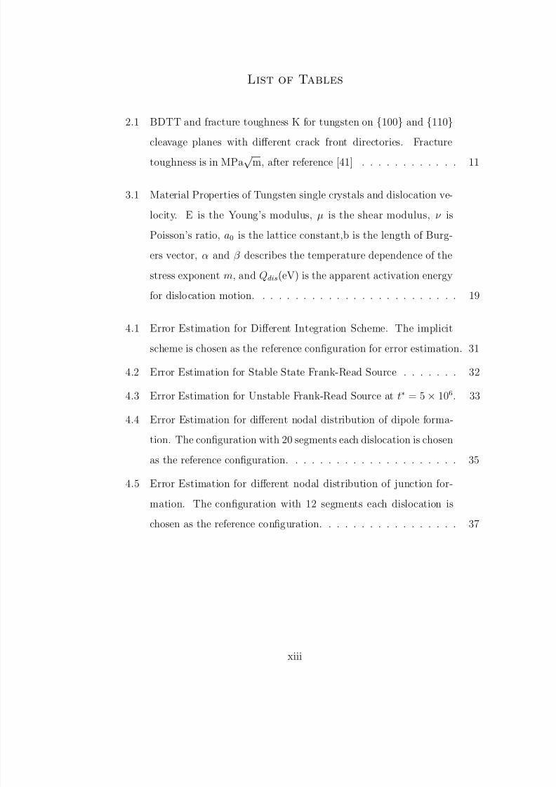
List of Tables
2.1 BDTT and fracture toughness K for tungsten on {100} and {110}cleavage planes with different crack front directories. Fracture
toughness is in MPa√
m, after reference [41] . . . . . . . . . . . . 11
3.1 Material Properties of Tungsten single crystals and dislocation ve-
locity. E is the Young’s modulus, µ is the shear modulus, ν is
Poisson’s ratio, a0 is the lattice constant,b is the length of Burg-
ers vector, α and β describes the temperature dependence of the
stress exponent m, and Qdis(eV) is the apparent activation energy
for dislocation motion. . . . . . . . . . . . . . . . . . . . . . . . . 19
4.1 Error Estimation for Different Integration Scheme. The implicit
scheme is chosen as the reference configuration for error estimation. 31
4.2 Error Estimation for Stable State Frank-Read Source . . . . . . . 32
4.3 Error Estimation for Unstable Frank-Read Source at t∗ = 5 × 10⁶. 33
4.4 Error Estimation for different nodal distribution of dipole forma-
tion. The configuration with 20 segments each dislocation is chosen
as the reference configuration. . . . . . . . . . . . . . . . . . . . . 35
4.5 Error Estimation for different nodal distribution of junction for-
mation. The configuration with 12 segments each dislocation is
chosen as the reference configuration. . . . . . . . . . . . . . . . . 37
xiii

8/8/2019 Dbt Thesis Ucla
http://slidepdf.com/reader/full/dbt-thesis-ucla 15/116
Acknowledgments
First of all, my deepest appreciation goes to my academic advisor, Professor Nasr
Ghoniem for his generous support and guidance during the past five years, hisdetailed suggestion and instruction is invaluable. Then, my thanks go to Dr.
Silvester Noronha, Xueli Han for the valuable discussions and help. I also extend
my thank to all my fellow students in the Nano & Micromechanics Laboratory
xiv
8/8/2019 Dbt Thesis Ucla
http://slidepdf.com/reader/full/dbt-thesis-ucla 16/116
Vita
1972 Born, Nantong, China.
1996 B.S., Science,Department of Mechanics & Mechanical Engineer-
ing University of Science & Technology of China, Heifei, China
1999 M.E., Department of Engineering Mechanics
Tsinghua Univeristy, Beijing, China
2003 Ph.D, Department of Mechanical and Aerospace Engineering
University of California, Los Angeles, Los Angeles, California
Publications
N.M. Ghoniem and J. Huang, Computer Simulations of Mesoscopic Plastic De-
formation with Differential Geometric Forms for the Elastic Field of Parametric
Dislocations : Review of Recent Progress, J. de Physique IV ,11(5) 53-60 (2001)
Jianming Huang and Nasr M. Ghoniem, The Dynamics of Dislocation Interaction
with Sessile Self-Interstitial Atom(SIA) Defect Cluster Atmospheres, J. Comp.
Mat. Science, 23 ,225-234 (2002).
N.M. Ghoniem, J. Huang, and Z. Wang, Affine Covariant-contravariant Vector
Forms for the Elastic Field of Parametric Dislocations in Isotropic Crystals, Phil.
Mag. Lett., 82(2): (2002)
xv

8/8/2019 Dbt Thesis Ucla
http://slidepdf.com/reader/full/dbt-thesis-ucla 17/116
N. M. Ghoniem, S.H. Tong, J. Huang, B.N. Singh, and M. Wen, Mechanisms
of Dislocation-Defect Interactions in Irradiated Metals Investigated by Computer
Simulations, J. Nucl. Mater., 307-311, 843-851 (2002)
Jianming Huang and Nasr M. Ghoniem, Accuracy & Convergence of Parametric
Dislocation Dynamics (PDD), Mod. Sim. Mat. Sci. Engr., 11, 21-39 (2003)
xvi
8/8/2019 Dbt Thesis Ucla
http://slidepdf.com/reader/full/dbt-thesis-ucla 18/116
Abstract of the Dissertation
Microstructural Effect on the Ductile-to-Brittle
Transition in Body Centered Cubic MetalsInvestigation by Three Dimensional Dislocation
Dynamics Simulations
by
Jianming Huang
Doctor of Philosophy in Mechanical and Aerospace Engineering
University of California, Los Angeles, 2004Professor Nasr M. Ghoniem, Chair
The Ductile-to-Brittle Transition(DBT) is a phenomenon that is widely ob-
served in Body Centered Cubic(BCC) metals and in covalently-based materials.
Below a critical temperature (DBTT), the material suddenly loss ductility. The
controlling mechanism of this transition still remains unclear despite of large
efforts made in experimental and theoretical investigation. Dislocation based
theories have been used to explain this phenomena. These fall into two broad
categories based on either nucleation of dislocation at crack-tips, or mobility
become higher at higher temperature.
Due to the limitation on the basic dislocation dynamics tool, all the previous
numerical work is based on two-dimensional dislocation theory. In this work, the
Parametric Dislocation Dynamics(PDD) method is reviewed and its key features
examined. They are: utilization of a small number of degree of freedom, high
accuracy, and high convergence rates. Applications of the PDD are demonstrated
to the determination of the flow stress in irradiated materials and to the inves-
xvii
8/8/2019 Dbt Thesis Ucla
http://slidepdf.com/reader/full/dbt-thesis-ucla 19/116
tigation of the mechanism of Persistent Slip Band(PSB) formation under fatigue
condition.
The interaction of dislocation and crack is a key part to understand the shield-
ing effect of the dislocation to the crack tip. A three dimensional discrete crack
dislocation distribution method based on PDD is proposed to solve for any kind
of crack tip field. By way of simulating the equilibrium distribution of the crack
dislocations under the applied load and their mutual interactions, crack tip stress
field can be easily obtained according to these crack dislocations. When the stress
field of the crystal dislocation is treated as external load, by modifying the dis-
tribution of the crack dislocation, the shielding effect can be easily obtained.
Dislocations are assumed to nucleated from different site, by way of coalescing,
generates longer dislocation to shield the whole crack front, and there is a transi-
tion zone of 3D to 2D simulation when the dislocation is far away from the crack.
At lower temperature, lower dislocation mobility prohibit the dislocation leaving
the crack tip region fast, and thus inhibit the instantaneous nucleation of further
dislocations, thus determines the fracture toughness of the considered material,
and as a result, the ductility or brittleness.
xviii

8/8/2019 Dbt Thesis Ucla
http://slidepdf.com/reader/full/dbt-thesis-ucla 20/116
CHAPTER 1
Introduction
Large scale ferritic steel structures, are used in pressure vessels, fusion reactor
structures, and in the construction of nuclear reactors. After a service period,
the originally ductile material may abruptly become brittle, and break without
pre-warning. This kind of abrupt transition in the level of ductility is unaccept-
able in engineering applications, because it may cause loss in economic. Thus
understanding the triggering mechanism of of such kind of transition is of great
importance.
Materials are not intrinsically perfect, since during manufacturing and pro-
cessing, micro voids and cracks are unavoidable. Under external loading, stresses
around these micro-cracks tend to be higher, causing their propagation. In most
metals, extensive plastic deformation is generated around the crack tip, absorb-
ing most of the external loading energy. In some other materials, like ceramics,
ice, Body Centered Cubic(BCC) metals at low temperatures, the applied exter-
nal energy can only be absorbed by way of extending the crack surface, causing
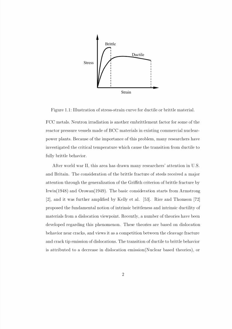
the propagation of crack and final failure of the material. Figure 1.1 shows two
types of stress-strain relations. According to their ability to generate plastic
deformation, materials can be classified as ductile or brittle.
The ductility of some materials can change with the environment. In some
BCC metals (e.g. W, α − F e) and some alkali halide, the ductility tends to be
lower as the temperature decreases. This kind of behavior is not observed in
1
8/8/2019 Dbt Thesis Ucla
http://slidepdf.com/reader/full/dbt-thesis-ucla 21/116
Brittle
Ductile
Strain
Stress
Figure 1.1: Illustration of stress-strain curve for ductile or brittle material.
FCC metals. Neutron irradiation is another embrittlement factor for some of the
reactor pressure vessels made of BCC materials in existing commercial nuclear-
power plants. Because of the importance of this problem, many researchers have
investigated the critical temperature which cause the transition from ductile to
fully brittle behavior.
After world war II, this area has drawn many researchers’ attention in U.S.
and Britain. The consideration of the brittle fracture of steels received a major
attention through the generalization of the Griffith criterion of brittle fracture by
Irwin(1948) and Orowan(1949). The basic consideration starts from Armstrong
[2], and it was further amplified by Kelly et al. [53]. Rice and Thomson [72]
proposed the fundamental notion of intrinsic brittleness and intrinsic ductility of
materials from a dislocation viewpoint. Recently, a number of theories have been
developed regarding this phenomenon. These theories are based on dislocation
behavior near cracks, and views it as a competition between the cleavage fracture
and crack tip emission of dislocations. The transition of ductile to brittle behavior
is attributed to a decrease in dislocation emission(Nuclear based theories), or
2

8/8/2019 Dbt Thesis Ucla
http://slidepdf.com/reader/full/dbt-thesis-ucla 22/116
due to the obstruction of the motion of dislocations(mobility based theories).
Thus dislocation dynamics becomes a useful tool to understand the behavior of
dislocation activities and their effects on crack tip.
First introduced in the 1980’s [63, 37], Dislocation Dynamics has now become
an attractive tool for investigations of the collective processes that constitute
plastic deformation of crystalline materials. In its earlier stage, numerical de-
scriptions of dislocation ensemble evolution have been examined in considerable
detail. Dislocations are approximated as 2-D and straight, making rigorous calcu-
lation of close-range interactions rather difficult. Recently, a number of numerical
simulation approaches have been developed which differ mainly in the represen-
tation of dislocation loop geometry, the manner of the calculation of the elastic
field and self-energy, and the description of boundary conditions. According to
these differences, these methods can be categorized as follows:
1. The Lattice Method:[58, 57, 18, 13, 56, 14, 20, 17, 19, 67] Straight segments,
either pure screw or edge in the earliest versions , or of a mixed character
in more recent versions, are allowed to jump on specific lattice sites and
orientations.
2. The Force Method:[45, 95] Straight segments of mixed character are moved
in a rigid body fashion along the normal to their mid-points. No information
of the elastic field is necessary, since explicit equations of interaction forces,
developed by Yoffe [94] are directly used.
3. The Differential Stress Method:[80, 78, 79] The stress field of a differential
straight line element on the dislocation is computed and integrated numer-
ically to give the necessary Peach-Koehler force. The Brown procedure [10]
is then utilized to remove the singularities associated with the self force
3

8/8/2019 Dbt Thesis Ucla
http://slidepdf.com/reader/full/dbt-thesis-ucla 23/116
calculation.
4. The Parametric Method:[60, 39, 40, 38] Dislocation loops are divided into
contiguous segments represented by parametric space curves. The equations
of motion for nodal attributes (e.g. position, tangent and normal vectors)
are derived from a variational energy principle, and once determined, the
entire dislocation loop can be geometrically represented as a continuous (to
second derivative) composite space curve.
5. The Phase Field Microelasticity Method:[54, 86] Based on Khachaturyan -
Shatalov(KS) reciprocal space theory of the strain in an arbitrary elasti-
cally homogeneous system of misfitting coherent inclusions embedded into
the parent phase, a consideration of individual segments of all dislocation
lines is not required. Instead, the temporal and spatial evolution of several
density function profiles (fields) are dealt with.
Based on the pioneer work of Eshelby in the 1950’s, and later developed by
Bibly, Cottrell and Swinden(BCS) [5], Bibly and Eshelby[4] and many others, a
continuous distributed dislocation technique for the simulation of crack problems
becomes an attractive alternative one. In this way, the elastic-plastic crack tip
field can be viewed as not only a distribution of dislocations on the crack plane,
but also a distribution of non-redundant dislocations within the plastic zones
of the crack tip, which in general can be viewed as the interaction of different
kinds of dislocations. For clarity, we name here the dislocation on crack plane as
crack dislocation , and real dislocations in the plastic zone around the crack tip
as crystal dislocation . So far, two dimensional crack has been extensively studied
by continuous crack dislocation distribution method, which leads to solving the
singular integral equations, but neither the numerical nor analytical solution for
4

8/8/2019 Dbt Thesis Ucla
http://slidepdf.com/reader/full/dbt-thesis-ucla 24/116
the equations can be easily solved when dealing with real crack and dislocation
interactions in three dimensional space. In this work, we proposed a discrete
dislocation distribution (DDD) Method based on Parametric Dislocation Method
(PDD) to avoid solving the hyper singular equations, and based on this, we
will studay the effect of the dislocation motion ahead of crack tip, as an aid to
understand the material ductility changes.
In what follows, in Chapter 2 we will survey the experimental methods and
data on the ductile-to-brittle transition behavior. In Chapter 3, current two
dimemsional BDT theories will be discussed. Our research progress on 3-D dislo-
cation dynamics will be presented in Chapter 4. The details of the DDD method
for the simulation of general three dimensional crack is given in Chapter 5. The
interaction of crack and dislocations as well as the temperature effect on the mo-
tion of the dislocations and the changes of the fracture toughness ahead of crack
tip is given in Chapter 6, and finally conclusion and future directions is given in
Chapter 7.
5

8/8/2019 Dbt Thesis Ucla
http://slidepdf.com/reader/full/dbt-thesis-ucla 25/116
CHAPTER 2
An Overview of Experiment Investigation of
DBTT on Single Crystals
Temperature and strain rate sensitive transitions are generally determined by the
competition between cleavage fracture mechanism and dislocation activity in the
region of crack tip. Due to the limitation on mesoscopic theories on polycystalline
materials, most experiments are based on single crystals. It is found that the
Ductile-to-Brittle transition(DBT) in single crystal materials can be classified
into two categories, as shown in FIG. 2.1.
A p pl i e d L o a d
Temperature
Fracture Yield
Increasing dK/dt
(a) (b)
A p pl i e d L o a d
Temperature
Fracture Yield
Increasing dK/dt
Figure 2.1: Two types of ductile brittle transition in single crystals.(a) soft tran-
sition (b) sharp transition[73]
1. Soft transition: The stress intensity factor for fracture rises over a wide
temperature range. This rise is due to the increase in dislocation activity
6

8/8/2019 Dbt Thesis Ucla
http://slidepdf.com/reader/full/dbt-thesis-ucla 26/116
at the crack tip with the temperature changes. This type of transition
is displayed by germanium [82], MgO [7], zirconia[65], molybdenum[23],
titanium aluminide[6], nickel aluminide[81, 3], tungsten[49].
2. Sharp transition: The transition occurs within a small range of tempera-
tures, usually within 10◦C . Below the transition temperature Tc, the stress
intensity factor K almost keeps as a constant value, around KIC , but when
temperature is enhanced above this critical value, there is a sharp increase
in material ductility as shown in the figure the sharp increase in the applied
load to causing fracture. This may due to the outburst of dislocation around
the crack tip zone. This kind of phenomenon is observed in Si[51, 77, 8],Al[55].
It is also shown in FIG. 2.1 that the loading rate dK/dt have strong effect
on BDTT, higher dK/dt may cause the increase in BDTT. It is shown that
the transition type of DBT is strongly dependent on the initial distribution of
dislocation sources [87], sharp transitions can only occur in initially dislocation
free materials.
2.1 Silicon
Silicon is generally used as an experimental material, because of the availabil-
ity of well-characterized dislocation-free crystals with known dopant levels. St.
John[51] is the first to study crack tip dislocation activities by testing a tapered
double cantilever beam specimen at different temperatures. In his experiments,he found that BDT occurs within a very narrow temperature range (i.e. sharp
transition) and BDTT is rate dependent with an activation energy of 1.9 eV over
the temperature range from 973 to 1223K. Michot et. al. (1980), Michot(1982),
7
8/8/2019 Dbt Thesis Ucla
http://slidepdf.com/reader/full/dbt-thesis-ucla 27/116

8/8/2019 Dbt Thesis Ucla
http://slidepdf.com/reader/full/dbt-thesis-ucla 28/116
tion can be nucleated continuously from crack tips, they cannot move deep into
the specimen to generate effective shielding. Furthermore, due to the free crack
surface, image forces will draw these out of the surface in high temperature en-
vironments. Also in their experiment, it is shown that reaching the crack arrest
temperature does not always cause general yielding. And if loading is continued,
ductile to brittle transition can still happen. After crack arrest, continuous load-
ing will cause a competition between the loading rate and the expansion rate of
the crack tip plastic zone. When the rate of crack tip plastic zone (or motion of
the dislocation) is lower than the loading rate, cleavage fracture was shown to
still occur.
P
1
2
3
4
5
1aD
iaD
arrest
d
end of chevron
d P
Oa
54321
a BDT T =
iT
d a d
d t d t
dµ
(a)(b)
Figure 2.2: Depiction of a relatively idealized jerky crack advance scenario in
which the stepwise advancing crack is systematically put into new environments
at progressively increasing temperature until it is eventually arrested. After ref-
erence [30]
Recently, Gally and Argon [30] abandoned the constant displacement rate inHsia and Argon’s experiment [47] due to its high sensitivity to minor perturba-
tions. They used a double cantilevel-beam(DCB) geometry specimen to test the
DBTT since the crack is intrinsically stable due to the crack tip stress intensity
9

8/8/2019 Dbt Thesis Ucla
http://slidepdf.com/reader/full/dbt-thesis-ucla 29/116
1410-
1310-
1.82u eV D =
11/ ( )
BDT K
-7.5 8 8.5 9
410-´
0V
Figure 2.3: Dependence of the brittle-to-ductile transition temperature T BD on
the average non-dimensional crack velocity v0. After reference [30]
decreasing with increasing crack length. There is a temperature gradient on the
specimen from low temperature at the initial crack tip to a critical temperature
at the place where a travelling crack with a given velocity can arrest. The tem-
perature was given by a series of up to ten thermocouples attached to the crack
face of the specimen which can give excellent agreement with the numerical heat
transfer solution, and the correction of the temperature was measured directly.
In their experiment, shown in FIG. 2.2, a stepwise advancing crack is systemat-
ically put into new environment at higher temperatures, and during each step,
dislocations will be possibly generated and followed by their multiplication and
expansion, which leads to crack shielding and blunting. FIG. 2.3 shows the rela-
tionship between the normalized average crack velocity v0 and T BD . Here, v0 is
defined as :
v0
= ∆a
∆tf
1
c=
∆af δ̇
cΛ ≈exp−
∆U
kT BD (2.1)
where, ∆af stands for final crack jump length, c stands for shear wave velocity,
Λ is the characteristic DCB dimension, δ is the pin displacement, ∆U is the
10

8/8/2019 Dbt Thesis Ucla
http://slidepdf.com/reader/full/dbt-thesis-ucla 30/116
Table 2.1: BDTT and fracture toughness K for tungsten on {100} and {110}cleavage planes with different crack front directories. Fracture toughness is in
MPa√
m, after reference [41]
Crack System BDTT(K) K at room temperature K at 77K
{100} < 010 > 470 8.7 3.4
{100} < 011 > 370 6.2 2.4
{110} < 11̄0 > 430 20.2 3.8
{100} < 001 > 370 12.9 2.8
activation energy. In their experiment, the activation energy is measured to be
1.82 eV which is considerably lower than most of the reported activation energies
of 2.2 eV for dislocation glide. This may due to the inaccuracy in measuring the
final period ∆tf . By way of combining etch pitting and Berg-Barrett imaging,
they also find that there is an inclination of choosing only one slip activity on a
set of two symmetrically placed vertical slip planes.
Argon and Gally [1] in their fracture experiments with dislocation-free Si
single crystals finally pointed that, while the overall B-D fracture transition bycrack arrest is indeed governed by the mobility of a very large group of dislocations
moving away from the crack tip. These dislocations can be easily generated from
the crack front cleavage ledges with lower energy barriers.
2.2 Tungsten
Gumbsch et al. [41] in their experiments examined the brittle-to-ductile transitionbehavior in tungsten single crystals. In their three point bend experiments, four
crack systems: {100} < 010 >, {100} < 011 >, {110} < 11̄0 >, {100} < 001 >
11

8/8/2019 Dbt Thesis Ucla
http://slidepdf.com/reader/full/dbt-thesis-ucla 31/116
Figure 2.4: Loading rate K̇ dependence of fracture toughness K of a specimen
with {110}< 11̄0 > crack system. Triangles, K̇ = 0.1 MPa m1/2/s; squares, K̇=
0.4 MPa m1/2/s; circles, K̇= 1.0 MPa m1/2/s. After reference [41].
were carefully examined. The temperature range covered from liquid nitrogen
temperature(77 K) to 650 K, and the test was performed at the constant loading
rate 0.10±
0.02 MPa√
m/s. The corresponding BDTT of different crack systems
is shown in Table 2.1. It is shown that for all the four systems, the BDTT
falls into an interval of 100 K. It is also shown in FIG 2.4 that the high loading
rate always lowers the fracture toughness, while increasing the BDTT, this is
consistent with what Roberts et al’s estimation [73]. The activation energy is
tungsten is measured as QBDT ≈ 0.2 eV. Chemical etching with an aqueous
solution of K3Fe(CN)6 and NaOH makes the process of dislocation penetrating
at fracture surface visible. In their experiment, motion of dislocations around thecrack tip is clearly shown with this method. At higher temperature, there is an
increase in the dislocation population, which suggest that additional sources are
activated compared with precracked specimens. Also, Gumbsch et al argue that
12
8/8/2019 Dbt Thesis Ucla
http://slidepdf.com/reader/full/dbt-thesis-ucla 32/116
at low temperature, dislocation nucleation is limited because of the scarcity of
active sources, while increasing the temperature sufficiently will activate a large
number of sources. Dislocation mobility assumes to control the nucleation rate
and thus the fracture toughness becomes rate dependent. And it is evident that
any model for BDT cannot be based on nucleation while excluding dislocation
mobility. In their whole temperature regime of investigation , it is shown that
the main controlling effect of BDT is the dislocation mobility.
2.3 Experiments on Effect of Alloying
Pure Cr
I*
III
I
210
100
0
-100
DBTT(0C)
Solute Concentration (%)
II
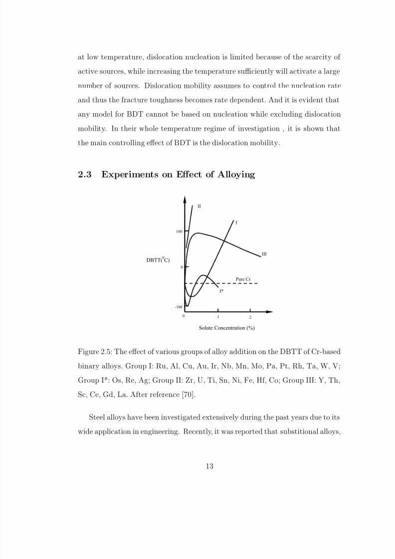
Figure 2.5: The effect of various groups of alloy addition on the DBTT of Cr-based
binary alloys. Group I: Ru, Al, Cu, Au, Ir, Nb, Mn, Mo, Pa, Pt, Rh, Ta, W, V;
Group I*: Os, Re, Ag; Group II: Zr, U, Ti, Sn, Ni, Fe, Hf, Co; Group III: Y, Th,
Sc, Ce, Gd, La. After reference [70].
Steel alloys have been investigated extensively during the past years due to its
wide application in engineering. Recently, it was reported that substitional alloys,
13

8/8/2019 Dbt Thesis Ucla
http://slidepdf.com/reader/full/dbt-thesis-ucla 33/116
interstitial alloys and alloys containing precipitates and second-phase inclusions
can cause the so called solid-solution softening at low temperatures, hence the
DBTT is somewhat different from pure metals, although that is not necessarily
due to alloy softening(AS) [70]. FIG. 2.5 shows the change in DBTT with the
solute concentration of Cr-based alloys with high purity. It is shown that most
of the solutions result in the loss of ductility of alloyed Cr (i.e. increase in
DBTT). For group II and III solutions, the ductility of Cr-based alloy was found
to decrease with an increase in the solute concentration. The reason is still
unclear.
Ductile crack growth initiated by the formation of disconnected ductile mi-
crocracks can be found in most of steel alloys. However, the mechanism of the
formation of microvoids and their spacial distribution ahead of the crack tip
maybe different. Recently, Ebrahimi and Seo [22] investigated crack initiations
in a two specific type of steels: a ferritic-pearlitic and a bainitic structural steel.
In the ferritic-pearlitic steel, relatively large inclusions, mainly manganese sulfide,
were found to be close to the crack tip, where microvoids may form due to high
shear stresses, Ductile cracks usually grow along the position of these particles.
For bainitic steels, geometrical inhomogeneities was found to be the main reason
for the formation of local microcracks.
As discussed in detail by Xu et al. [90, 91], α − F e has little or no energy
barrier to kink motion along dislocation lines, thus the triggering effect of BDT
is primarily through the formation of a dislocation embryo at the crack tip. This
mechanism is different from crack behavior in silicon single crystals as discussed
previously.
14
8/8/2019 Dbt Thesis Ucla
http://slidepdf.com/reader/full/dbt-thesis-ucla 34/116
CHAPTER 3
Review of Current Theoretical Modelling
Many methods have been proposed to analyze the transition phenomenon, most of
them show the intimate connection between the dislocation activity near the crack
tip and fracture toughness. Among them, there are basically two groups. The first
group is based on dislocation nucleation, and assume that dislocation nucleation
at the crack tip is the controlling factor in the DBT. This is the characteristic
of BCC transition metals. Another category is mobility-based models, which
basically assume that dislocation nucleation is relatively easy, while temperature
affects the motion of dislocations. The back stress due to these dislocations at
the crack tip affects the fracture toughness. This behavior is typical of semi-
conductors and compounds. The distinguishing aspect between the two models
is the mobility of kinks on dislocations. Computer simulations show that the
kink motion along dislocations is hindered by very substantial energy barriers
in Si. In some experiments, it is indicated that there is little resistance to the
motion of kinks along dislocation lines in some BCC metals. These suggest that
the transition is either controlled by nucleation (BCC materials) or is mobility
controlled.
15

8/8/2019 Dbt Thesis Ucla
http://slidepdf.com/reader/full/dbt-thesis-ucla 35/116
Dislocation
emission
0r
Cleavagec
g
Figure 3.1: Illustration of Rice-Thomson model.
3.1 Nucleation-based Models
Rice and Thomson [72] were the first to consider the brittle versus ductile be-
havior of materials in terms of crack tip dislocation activity. As shown in FIG.
3.1, they proposed that the competition between dislocation emission and atomic
decohesion at the crack tip is the controlling factor in the ductile versus brittle
behavior of a material. In their model, they assumed that there is an embryonic
dislocation nucleated on a gliding plane with inclination angle φ. The distance
between the embryonic dislocation and the crack tip is equal to the dislocation
core radius r0. Propagation of the crack will have two possibilities under exter-
nal stress. The first is that the nucleation of the embryonic dislocation and its
subsequent motion away from the tip, which makes the crack tip blunt. The
other is that cleavage fracture proceed along the crack surface, and the crack
tip remains sharp. The stress which causes the emission of the dislocation is
mainly composed of an external K-field, the image stress due to the proximity to
free crack surfaces, and any other stresses due to crack blunting. On the other
hand, the energy release rate G can cause the propagation of the crack, while the
surface energy γ c acts as a retarding force. In the loading process, if dislocation
16

8/8/2019 Dbt Thesis Ucla
http://slidepdf.com/reader/full/dbt-thesis-ucla 36/116
emission occurs earlier, then the material is assumed to be intrinsically ductile,
otherwise it is brittle. In their model, the Griffith criterion is used for cleavage
requirements. Rice and Thomson developed quantitative evaluations of the con-
ditions for dislocation emission from the near-tip region. It was shown that the
ratio µb/γ c (here γ c stands for surface energy, µ shear modulus, and b the length
of Burgers vector) was a good indicator of the ductile versus brittle response.
Materials whose dislocations have wide core and with small value in µb/γ c tend
to be ductile. The energy barrier to dislocation emission was calculated to be 19
eV for Fe, 329 eV for W, 111 eV for Si and 329 eV for Ge. Their values are much
higher than the experimentally found activation energies for BDT.
In experimental observations, dislocations are not always emitted as straight
long segments, as assumed in 2-D analysis shown in FIG. 3.1. Two dimensional
models always underestimate the material ductility. Recently, researchers con-
sider the initial dislocation loop configuration as rectangular or half elliptic, as
shown in FIG. 3.2. Three dimensional loop models not only predict the ductility
more precisely, but also decided the motion and configuration of dislocations after
their nucleation. Gao and Rice [31] studied the half elliptical case, and obtained
a lower K needed for the emission, as compared with the 2-D case. Later, the
Rice-Thomson model has evolved continuously, to account for elastic anisotropy,
bimaterial interfaces, nonlinear dislocation core structures, and realistic slip sys-
tem geometries. Xu, Argon and Otiz [91] in their paper studied different realistic
slip system geometries. The activation configuration includes nucleation on in-
clined planes, on oblique planes and on cleavage ledges, all of them are treated
within the framework of Peierls.
Xu et al [90] suggested that the possible B-D transition temperature from the
17

8/8/2019 Dbt Thesis Ucla
http://slidepdf.com/reader/full/dbt-thesis-ucla 37/116
(a) (b)
Figure 3.2: 3-D dislocation nucleation models from crack tip. (a) rectangular
loop. (b) elliptical loop
activation energy as:
T BD =
ln (c/v)
α+ η
T 0T m
−1T 0 (3.1)
Here, T 0 = µb3/k(1 − ν ) ≈ 1.2 × 10⁵K , the melting temperature T m = 1809 K
for α-Fe, α = (1 − ν )∆U activation/µb3 is the normalized activation energy, c is
the speed of sound, v≈
1 cm/s is the typical crack propagation velocity, giving
ln(c/v) ≈ 10, η ≈ 0.5 is a coefficient describing the temperature dependence
of the shear modulus. Thus, BDTT is dependent on the activation energy of
dislocation nucleation.
3.2 Mobility-based Models
In many materials, such as BCC metals, the dislocation velocity increases stronglywith the temperature increase till the so-called athermal temperature. Above this
temperature, the dislocation velocity is widely temperature independent. Below
this temperature, the dislocation velocity is regarded as being thermally activated
18

8/8/2019 Dbt Thesis Ucla
http://slidepdf.com/reader/full/dbt-thesis-ucla 38/116
Table 3.1: Material Properties of Tungsten single crystals and dislocation velocity.
E is the Young’s modulus, µ is the shear modulus, ν is Poisson’s ratio, a0 is
the lattice constant,b is the length of Burgers vector, α and β describes the
temperature dependence of the stress exponent m, and Qdis(eV) is the apparent
activation energy for dislocation motion.
E(GPa) µ(GPa) ν a0(nm) b(nm) α(K) β A(m/s) Qdis(eV)
388.7 152.7 0.29 0.3159 0.274 592 2.81 3.23 × 10⁻⁹ 0.323
with some activation energy Qdis, and can be written in the Arrhenius-type form
v = A τ
τ 0m(T )
exp−
Qdis
kBT
(3.2)
Where A is a constant with the dimension of velocity, τ is shear velocity exerted
on the dislocation, τ 0 is normalized stress, kB is Boltzmann’s constant, T is the
absolute temperature. m (T ) is the temperature dependent constant, assumed to
be of the form [71]
m(T ) =α
T + β (3.3)
α and β are the two fitted constants. Table 3.1 lists all the parameters for
Tungsten dislocation velocity.
Let’s define dislocation mobility as
M = A exp−U v
kBT
then EQN. 3.2 can be rewritten as:
v = Mτ m
(3.4)
As can be seen from EQN. 3.4, the higher the total shear stress applied on the
dislocation, the faster the dislocation moves. On the other hand, the higher
19

8/8/2019 Dbt Thesis Ucla
http://slidepdf.com/reader/full/dbt-thesis-ucla 39/116
the temperature, the higher mobility of the dislocation, and thus the higher the
dislocation velocity. At a given temperature, once the dislocation velocity is
determined, and the external loading and internal interactions between disloca-
tions are also set, then the position of the dislocation will be known. Thus, the
shielding effect of the dislocations to the crack is known, and hence the local
stress intensity factor is determined. Applying the Griffith criterion, the critical
condition for crack propagation can be determined at any temperature. Numeri-
cal simulations show that the transition temperature is highly dependent on the
loading rate[42].
The other category of models consider that the mobility is constant, while the
total stress on the dislocation changes at different temperatures due to a change in
the Peierls-Nabarro stress. The Peierls-Nabarro stress is defined as the applied
resolved shear stress required to overcome the lattice resistance to movement
by a dislocation loop. The Peierls stress is a consequence of the inter-atomic
forces/displacement interaction between the dislocation loop and the surrounding
crystals. And this resistance to dislocation movement is due to the periodic
variation in the misfit energy of atomic half planes above and below the slip plane
with the dislocation loop. For higher dislocation densities, the Perierls stress
is comparable to long range interactions between dislocations. It is generally
accepted that the Peierls stress is a dominant controlling factor in the plastic slip
at low temperatures [84]. It decreases with an increase in temperature. Thus the
effect of temperature on the Peierls stress can also help us understand the BDT
phenomenon.
20

8/8/2019 Dbt Thesis Ucla
http://slidepdf.com/reader/full/dbt-thesis-ucla 40/116
3.3 Current Computer Simulations and their limitations
With the fast development of the computer technique, more and more people
tend to use numerical method to simulate the plastic deformation in mesoscopicscale. Dislocation Dynamics (DD) has now become an attractive tool for inves-
tigations of the ductile to brittle transition process, but most of them concen-
trated on the interaction on infinite straight dislocation with 2D cracks, which
may underestimate or overestimate the BDT temperature. The Oxford group
[42, 74, 45, 75] and related references, Xin and Hsia [89], Ferney and Hsia [26],
carefully studied the BDTT on Si in 2D, and concluded that the BDT in silicon
is mainly controlled by dislocation mobility, based both on peripheral evidence
that the activation energy for the transition temperature is the same as that for
dislocation mobility.
The basic procedure for the simulation is straightforward as shown in the
following several steps:
1. Calculate the total stress on the dislocation
The total stress applied on the ith dislocation τ i can be written as follow:
τ i = τ iK + τ iimage + τ iinteraction + τ iother (3.5)
Here, τ iK is the shear stress due to crack tip stress field, usually they are
written as follow:
τ iK =K applied√
πrif (θ) (3.6)
Here, ri
is the distance toward the crack tip, f (θ) is the coefficient related
to the inclination angle of the slip plane. Usually, 2D K-field is considered.
For the image stress τ iimage, direct analytical results for infinite straight long
21

8/8/2019 Dbt Thesis Ucla
http://slidepdf.com/reader/full/dbt-thesis-ucla 41/116
solution is used,
τ iimage = β µb
ri(3.7)
β is a correction coefficient.
The dislocation-dislocation interaction term τ iinteraction can be written as
[89]:
τ iinteraction =µb
4π(1 − ν )
j=i
ri
r j
1/21
ri − r j+
8rir j
(ri + r j)3 (ri − r j)
(3.8)
Summing up all the stress term related to dislocation and crack, also stresses
generated by grain boundary, or other impurities, we can get the net shear
stress on the dislocation.
2. Update the positions of each dislocation
According to EQN 3.4, calculate the new position of each dislocation at a
small time step by way of any implicit or explicit integration method.
3. Update the locale stress intensity factor K
K total = K applied − K D (3.9)
Here,K D is the factor of the dislocations, and can be written as follows:
[26, 43]
K D =i
µbf (θ)
(2πri)1/2 (1 − ν )
(3.10)
Here, f (θ) is a coefficient related with slip direction and different slip sys-
tem, in different simulation conditions, this value may vary. In [89], this
value is chosen as 3√2/4α where, α is the number of equivalent active slipsystems, referring as the shielding coefficient, for instance, α = 2 means
that two symmetric slip systems are activated, and α = 1 means that only
one slip system is activated. In their results, it is shown that increasing
22

8/8/2019 Dbt Thesis Ucla
http://slidepdf.com/reader/full/dbt-thesis-ucla 42/116
the number of active slip systems will lead to a sharp transition, and the
sharpness is strongly dependent on α. When α = 4, the transition may
become extremely sharp. It is argued that with lower α = 1, the number
of dislocations at the moment of cleavage fracture increases gradually over
a wide temperature range, whereas for large values of α, there is a sudden
increase in the number of dislocation accompanied by sharp transition.
4. Check the dislocation emission condition
Similar to the Rice-Thomson model[72], embryonic dislocations exist at
r = rc from the crack tip, where rc is the core radius, once the crack tip
stress intensity factor reaches a critical value, one dislocation is emitted.
Note here that, emission of new dislocation doesn’t depend on the presence
of prior ones.
5. Apply the fracture criteria
For brittle fracture, according to Griffith criterion, check the stress intensity
K total whether it exceeds the intrinsic fracture toughness K IC , or for ductile
fracture[89], when the far applied field K applied, exceed some certain limit,7K IC is chosen in [89]. If both two conditions are not satisfied then go back
to step 1, and continue on the computational cycle.
FIG. 3.3 shows a typical simulation model. FIG. 3.3a shows a truly 2-D
problem with straight dislocations and 2-D crack tip field, and in FIG. 3.3b, a
pseudo 3D case are studied, where dislocations can be emitted from position near
crack fronts with rectangular shape, and during their motion, the 3 segment of
the dislocation still keeps as straight.
As previously discussed, the limitations are obvious. First, in reality, there is
no straight dislocations, so for the Dislocation Dynamics(DD) part, it is difficult
23

8/8/2019 Dbt Thesis Ucla
http://slidepdf.com/reader/full/dbt-thesis-ucla 43/116
as
Source
Dislocation
crit d 2
as
Source
Dislocation
(a)(b)
Figure 3.3: Modelling the plastic zone as a single inclining slip plane (a) uniform
dislocation nucleation (b) dislocation nucleation at separated sources. refer to
[43]
to simulate real 3D configurations, and especially difficult to solve for the dislo-
cation motion at earlier stage, since their shielding effect is stronger, due to their
short distance to the crack tip. And for 2D case, it is difficult to estimate the
effect of different slip systems as discussed in Xu and Argon’s work[91]. How is
the mutual interactions between those dislocations in different slip planes? For
2D simulation, it is impossible to answer this question clearly. Second, is the
calculation the applied K -field, since most of the problem can not be simplified
to two dimension.
24

8/8/2019 Dbt Thesis Ucla
http://slidepdf.com/reader/full/dbt-thesis-ucla 44/116
CHAPTER 4
Computational Aspect of Parametric
Dislocation Dynamics
Dislocation Dynamics (DD) has now become an attractive tool for investigations
of both fundamental and collective processes that constitute plastic deformation
of crystalline materials. Since it is a foundational issue in studying the dislocation
emission and motion ahead of crack tip, we here have a detailed review of the
three dimensional parametric dislocation dynamics and its numerical accuracy
and convergence.
4.1 Formulation of Parametric Dislocation Dynamics (PDD)
The method of PDD is described in sufficient details in references [36, 39, 40,
38], and we will attempt here to give only a brief description. The first step is
to calculate the stress field of curved parametric segments. Let the Cartesian
orthonormal basis set be denoted by 1 ≡ {1x, 1y, 1z}, I = 1 ⊗ 1 as the second
order unit tensor, and ⊗ denotes out tensor product. Now define the three
vectors (g1 = e, g2 = t, g3 = b/|b|) as a covariant basis set for the curvilinear
segment, and their contravariant reciprocals as[46]: gi
· g j = δi
j, where δi
j is themixed Kronecker delta and V = (g1 × g2) · g3 the volume spanned by the vector
basis, as shown in FIG. 4.1 . The parametric representation of a general curved
25
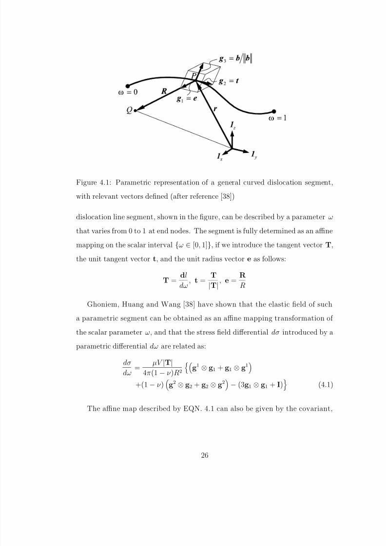
8/8/2019 Dbt Thesis Ucla
http://slidepdf.com/reader/full/dbt-thesis-ucla 45/116
Figure 4.1: Parametric representation of a general curved dislocation segment,
with relevant vectors defined (after reference [38])
dislocation line segment, shown in the figure, can be described by a parameter ω
that varies from 0 to 1 at end nodes. The segment is fully determined as an affine
mapping on the scalar interval {ω ∈ [0, 1]}, if we introduce the tangent vector T,
the unit tangent vector t, and the unit radius vector e as follows:
T =dl
dω
, t =T
|T|, e =
R
R
Ghoniem, Huang and Wang [38] have shown that the elastic field of such
a parametric segment can be obtained as an affine mapping transformation of
the scalar parameter ω, and that the stress field differential dσ introduced by a
parametric differential dω are related as:
dσ
dω=
µV |T|4π(1 − ν )R2
g1 ⊗ g1 + g1 ⊗ g1
+(1 − ν )
g2 ⊗ g2 + g2 ⊗ g2− (3g1 ⊗ g1 + I)
(4.1)
The affine map described by EQN. 4.1 can also be given by the covariant,
26

8/8/2019 Dbt Thesis Ucla
http://slidepdf.com/reader/full/dbt-thesis-ucla 46/116
contravariant and mixed vector and tensor functions [38]:
S = sym[tr(Ai.jgi ⊗ g j)] + A11(3g1 ⊗ g1 − 1 ⊗ 1) (4.2)
The scalar metric coefficients Ai
.j, A11
, B11
are obtained by direct reduction of EQN.4.1 into EQN.4.2. Once the parametric curve for the dislocation segment
is mapped onto the scalar interval {ω ∈ [0, 1]}, the stress field everywhere is
obtained as a fast numerical quadrature sum from EQN. 4.1 [39]. The self-force
is obtained from knowledge of the local curvature at the point of interest.
To simplify the problem, let us define the following dimensionless parameters:
r∗ =r
a
, f ∗ =F
µa
, t∗ =µt
BHere, a is lattice constant, µ the shear modulus, and t is time. Substitute these to
the variational formula of the governing equation of motion of a single dislocation
loop [40], we get the dimensionless matrix form as:
Γ∗
δr∗
f ∗ − dr∗
dt∗
|ds∗| = 0 (4.3)
Here, f ∗ = [f ∗1 , f ∗2 , f ∗3 ], and r∗ = [r∗1, r∗2, r∗3], which are all dependent on the
dimensionless time t∗. Following reference [40], a closed dislocation loop can be
divided into N s segments. In each segment j, we can choose a set of generalized
coordinates qm at the two ends, thus allowing parameterization of the form:
r∗ = CQ (4.4)
Here, C = [C1(ω), C2(ω),..., Cm(ω)], Ci(ω), (i = 1, 2,...m) are shape functions
dependent on the parameter (0 ≤ ω ≤ 1), and Q = [q1, q2,...,qm], qi are a set of
generalized coordinates. Now substitute EQN.4.4 into EQN.4.3, we obtain:
N s j=1
Γj
δQ
Cf ∗ − CC
dQ
dt∗
|ds| = 0 (4.5)
27

8/8/2019 Dbt Thesis Ucla
http://slidepdf.com/reader/full/dbt-thesis-ucla 47/116
Let,
f j = Γj
Cf ∗ |ds| , k j = Γj
CC |ds|
Following a similar procedure to the FEM, we assemble the EOM for all contigu-
ous segments in global matrices and vectors, as:
F =N s j=1
f j, K =N s j=1
k j
then, from EQN 4.5 we get,
KdQ
dt∗= F (4.6)
EQN. 4.6 represents a set of ordinary differential equations, which describe
the motion of an ensemble of dislocation loops as an evolutionary dynamical
system. Given the initial condition and boundary conditions, solving EQN. 4.6,
the position and configuration of each dislocation is set, and hence at each time
step, the total stress field can be known.
If we specifically choose cubic splines as shape functions, ignore the climbing
effect and confine dislocation motion to be on its glide plane, we end up with only
8 DOFs for each segment with each node associated with 4 independent DOFs.
These cubic spline shape functions are given by:
C = [2ω3 − 3ω2 + 1, ω3 − 2ω2 + ω, −2ω3 + 3ω2, ω3 − ω2]
Q = [P1, T1, P2, T2]
Here, Pi and Ti (i = 1, 2) correspond to the position and tangent vectors, re-
spectively.
28

8/8/2019 Dbt Thesis Ucla
http://slidepdf.com/reader/full/dbt-thesis-ucla 48/116
4.2 Spatial and Temporal Resolution of Dislocation Mech-
anisms
4.3 Temporal resolution
[-1 1 0]
[ - 1 - 1 2 ]
-500 0 5001200
1400
1600
1800
2000
2200
Implicit Integration
t*=3000
t*=1500
t*=1000
t*=500
b
Figure 4.2: The influence of the time integration scheme on the shape convergence
of an F-R source. Here, Burgers vector is chosen as 1/2[1̄01] with applied uniaxial
stress σ11 = 80 MPa. (or τ /µ = 0.064% )
As shown in previous section, after the initial conditions are set, the major
problem is to solve EQN. 4.6. Two kinds of integration methods, implicit and
explicit, are utilized. For the explicit integration, simple one step Euler forward
method are used. Modified Gear’s implicit integration for stiffness equation [35]
developed by Lawrence Livermore National Laboratory are used for implicit time
integration. The comparisons between implicit and explicit integrations with
different time steps are shown in FIG. 4.2, and error estimations at Table 4.1.
In the explicit scheme, it is noted that when the time step is larger than
≈ 3000, there will be a numerical shape instability. For the parameters chosen
29
8/8/2019 Dbt Thesis Ucla
http://slidepdf.com/reader/full/dbt-thesis-ucla 49/116
here, this corresponds to a physical time step of ≈ 6 ps. The shape tends to
diverge more along near screw segments of the F-R source. For a time step on
the order of 1000 (i.e. ∆t ≈ 2 ps), the F-R shape is numerically stable, but
not accurate. Finally, when the explicit time step is lowered to less than 500
(i.e. ∆t ≈ 1 ps), PDD tends to give a stable and accurate F-R source shape.
Such small limit on the time step for high mobility crystals (e.g. FCC metals)
can result in severe restrictions on the ability of current simulation for large
scale plastic deformation. With the method designed by Gear for the numerical
integration of ordinary differential stiff equations, a variable time step can be
automatically determined based on the variation of any of the DOF. A level
of relative accuracy of 10−6 is selected as a convergence constraint. Since the
time step is automatically adjusted to capture the specified level of accuracy,
the overall scheme is stable and convergent. It is shown in Table 4.1 that the
overall running time in explicit integration is much less than that with explicit
integration scheme at small time step. That is due to the ability of adjusting
time step during implicit integration according to the stiffness of the equation,
while explicit Euler method can’t, and only with very small time step can we get
the same level of accuracy and convergence.
4.4 Spatial resolution limits on PDD
For large-scale computer simulations, there is an obvious need to reduce the
computational burden without sacrificing the quality of the physical results. The
smallest number of spline segments with the largest time step increment for inte-
gration is a desirable goal. However, one must clearly identify the limits of this
approach. We study here the influence of the nodal density on the dislocation
line, and the time integration scheme on the ability to satisfactorily resolve the
30

8/8/2019 Dbt Thesis Ucla
http://slidepdf.com/reader/full/dbt-thesis-ucla 50/116
Table 4.1: Error Estimation for Different Integration Scheme. The implicit
scheme is chosen as the reference configuration for error estimation.
Integration Scheme Absolute Error a Relative Error r Runtime(sec)
Explicit Int.(∆t∗ = 3000) 168.4 6.11% 0.92
Explicit Int. (∆t∗ = 1500) 141.5 5.40% 1.82
Explicit Int. (∆t∗ = 1000) 56.90 2.34% 2.76
Explicit Int. (∆t∗ = 500) 0.06 0.003% 5.68
Implicit Integration 0 0 1.52
shape of a dynamic F-R source.
4.4.1 Single F-R source
FIG.4.3 shows a stable(with applied σ11 = 80 MPa, τ /µ = 0.064% ) and an un-
stable (σ11 = 200 MPa, τ /µ = 0.16%) F-R source configuration. The dislocation
loop is divided into different number of segments, and its motion is gained by
different numerical integrations. It is shown that one can achieve very high preci-
sion in describing the stable F-R shape with very small number of segments. The
corresponding error is shown in Table 4.2. For comparisons, we choose here the
result with 30 segments as the reference configuration(thus the relative and abso-
lute error is set to zero). It is found that with the increasing number of segments,
both the relative and absolute error are decreased sharply, but the running time
is increased significantly. It is interesting to note here that with only 2 segments,
one can achieve almost the same resolution as that with 30 segments, with the
relative error less than 0.2%, 2% of the CPU time used in 30 segments. However,
when the F-R source becomes unstable, the variation of curvature is considerable
31

8/8/2019 Dbt Thesis Ucla
http://slidepdf.com/reader/full/dbt-thesis-ucla 51/116
[-1 1 0]
[ - 1 - 1 2 ]
-500 0 5001200
1400
1600
1800
2000
22002 Segments
6 Segments
15 Segments
30 Segments
b
[-1 1 0]
[ - 1 - 1 2 ]
-4000 -2000 0 2000 4000 6000
0
2000
4000
6000
8000 2 Segments
6 Segments
15 Segments
30 Segments
40 Segments
(a) (b)
Figure 4.3: The influence of number of segments on the shape convergence of an
F-R source
between its middle section and the sections close to the pinning points, 2 segments
is not enough. FIG.4.3-b and Table 4.3 show the configuration and corresponding
absolute, relative error and running time respectively in the unstable case. The
reference configuration is chosen as that with 40 segments. It is found that only 2
segments is unable to achieve high accuracy, although it still converges. It is due
to the complicate configuration compared to that at stable case. The curvature
Table 4.2: Error Estimation for Stable State Frank-Read Source
No. of Segments Absolute Error a Relative Error r Runtime(sec)
2 6.06 0.17% 0.12
6 6.01 0.15% 0.42
15 1.32 0.018% 1.53
30 0 0 5.77
32

8/8/2019 Dbt Thesis Ucla
http://slidepdf.com/reader/full/dbt-thesis-ucla 52/116
Table 4.3: Error Estimation for Unstable Frank-Read Source at t∗ = 5 × 10⁶.
No. of Segments Absolute Error a Relative Error r Runtime(sec)
2 1408.8 20.15% 0.02
6 191.1 5.04% 0.20
15 133.8 3.24% 2.53
30 142.0 2.93% 24.14
40 0 0 27.57
is much higher at the zone near the fixed point. Only 2 segments is not enough
to capture such a high curvature, the error is mainly from these two zones. InTable 4.3, it is shown that with the increasing number of segments, the accuracy
increased greatly with the compensation of increasing CPU time.
4.4.2 Finite-Size Dipole Formation
FIG. 4.4 shows a 2-D projection on the (111)-plane of the dynamic process finite-
size dipole formation. Two initially straight dislocation segments with the same
Burgers vector 12
[1̄01], but of opposite line directions are allowed to glide on
nearby parallel {111}-planes without the applying an external stress. The two
lines attract one another, thus causing the two loop segments to move and finally
reach an equilibrium state of a finite-size dipole. The two parallel dislocations
are pined at both ends, the upper loop glides on the ”upper” plane, while the
”lower” one glides on the ”lower” one as shown in the figure. The mutual attrac-
tion between the two dislocations becomes significant enough to simultaneously
reconfigure both of them only during the latter stages of the process. Because
the two dislocations start with a mixed character, a straight and tilted middle
section of the dipole forms. The length of this middle section, which we may
33

8/8/2019 Dbt Thesis Ucla
http://slidepdf.com/reader/full/dbt-thesis-ucla 53/116
Figure 4.4: Two F-R source dislocations with the same Burgersvector(b = 1
2 [1̄01]) but opposite tangent vectors gliding on two parallel
(111)-planes (h = 25√
3a apart) form a short dipole in an unstressed state.
The view is projected on the (111)-plane. Time intervals are: (1) 2.5 × 10⁵,
(2) 4.75 × 10⁵, (3) 5 × 10⁵ , (4) Equilibrium state
34
8/8/2019 Dbt Thesis Ucla
http://slidepdf.com/reader/full/dbt-thesis-ucla 54/116
Table 4.4: Error Estimation for different nodal distribution of dipole formation.
The configuration with 20 segments each dislocation is chosen as the reference
configuration.
No. of Segments Absolute Error a Relative Error r Runtime(sec)
2 26.5 3.16% 12.7
4 18.6 2.37% 43.3
5 7.8 1.13% 84.9
10 3.6 0.36% 438.2
20 0 0 1503.1
simply ascribe as the dipole length, is only determined by the balance between
the attractive forces on the middle straight section, and the self-forces on the
two end sections close to the pinning points. The separation of the two planes is
25√
3, which is approximately 60 |b|.
The error estimation of different nodal distribution of same dipole formation
is shown in Table 4.4. It is shown that with only 2 segments in each dislocation,
high accuracy can be obtained, the relative error is less than 5%.
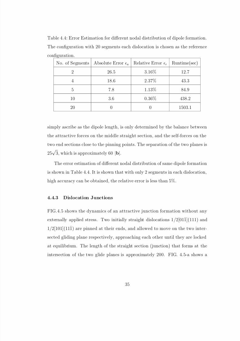
4.4.3 Dislocation Junctions
FIG.4.5 shows the dynamics of an attractive junction formation without any
externally applied stress. Two initially straight dislocations 1/2[011̄](111) and
1/2[101](111̄) are pinned at their ends, and allowed to move on the two inter-
sected gliding plane respectively, approaching each other until they are lockedat equilibrium. The length of the straight section (junction) that forms at the
intersection of the two glide planes is approximately 200. FIG. 4.5-a shows a
35
8/8/2019 Dbt Thesis Ucla
http://slidepdf.com/reader/full/dbt-thesis-ucla 55/116
2-D projection view of the successive motion of 12 [011̄](111) , while the 3-D view
of the junction structure is shown in FIG. 4.5-b. In order to calculate the error
generated by different nodal distribution, the configuration with 12 nodes each
dislocation is set as the reference one. The error estimation is shown in Table
4.5. It is shown that one can get good shape junction with less than 8 segments
in each dislocation loop.
[-1 1 0]
[ - 1 - 1 2 ]
-250 0 250 500
-200
-100
0
100
200
2345 1
[1 1 1]
[1 1 -1]
(a) (b)
Figure 4.5: Dynamics of 2 unstressed F-R sources ( 12 [011̄](111) and 1
2 [101](111̄))
forming a 3D junction along (1̄10) , b = 12
[110]. (a) 2D view for the motion of
the F-R source ( 12 [011̄](111)12 [1̄01](11̄1)) on its glide plane(111). Time intervals
are (1) initial configuration, (2) 1.5 × 10⁴, (3) 5.0 × 10⁴, (4) 1.3 × 10⁵, (5) Final
configuration. (b) 3-D view of the junction
4.5 Adaptive Node Redistribution
One of the main feature of our PDD is the adaptive algorithm of space division. In
order to capture details of small scale processes, such as the interaction between a
36

8/8/2019 Dbt Thesis Ucla
http://slidepdf.com/reader/full/dbt-thesis-ucla 56/116
Table 4.5: Error Estimation for different nodal distribution of junction formation.
The configuration with 12 segments each dislocation is chosen as the reference
configuration.
No. of Segments Absolute Error a Relative Error r Runtime(sec)
3 27.8 20.05% 406.2
4 19.7 14.25% 841.1
6 16.0 8.75% 2932.6
8 4.97 1.00% 4902.4
12 0 0 8320.2
dislocation and an atomic size defect cluster, or during the annihilation reaction
between two dislocation segments of the same Burgers vector and of opposite
tangent vector, large variations of the local dislocation line curvature would be
expected. To effectively resolve these or similar mechanisms, we develop here a
protocol for adaptively re-distributing of the nodal density on the dislocation line
according to the variation in the local curvature. To show the level of resolution
gained by this protocol, we study here the mechanism of dislocation segment
annihilation in an expanding F-R source, and the subsequent generation of a
fresh and closed dislocation loop.
In the annihilation event, the distance between any two nodes is tracked, and
once the minimum distance between two segments of opposite tangent vectors is
below a prescribed limit (e.g. 100), the two segment will annihilate, and generate
two separate loops one closed and one open. The nodes are re-distributed in the
immediate region, as can be seen in FIG. 4.6. The simulation conditions are the
same as in previous figure, except that the applied stress σ11 = 140 MPa(τ /µ =
0.112%), and the Burgers vector of the loop is b = 12 [01̄1].
37

8/8/2019 Dbt Thesis Ucla
http://slidepdf.com/reader/full/dbt-thesis-ucla 57/116
[-1 1 0]
[ -
1
- 1
2 ]
-5000 0 5000
-8000
-4000
0
4000
b
t*=0
Figure 4.6: Expansion of an initially mixed dislocation segment in an F-R source
under the step function stress of σ22 = 140 MPa(τ /µ = 0.112%). The F-R source
is on the (1 1 1)-plane of a Cu crystal with Burgers vector b = 12
[01̄1]. The time
interval between different contours is ∆t∗ = 5 × 10⁵.
38

8/8/2019 Dbt Thesis Ucla
http://slidepdf.com/reader/full/dbt-thesis-ucla 58/116
As shown in the figure, after the annihilation event takes place, both new
loops generate cusp regions, where the curvature is extremely high. In our com-
putational strategy, we developed an adaptive scheme to resolve such an essential
physical phenomena for sufficient accuracy without excessive computations.
In present algorithm, at prescribed time intervals, there will be a nodal re-
distribution process, it may not necessarily related to the integration time step.
During the redistribution process, each cubic spline segment is divided into sev-
eral sub-segments with equal arc length, and new ghost nodes are assigned. Thus,
the entire loop is now filled with ghost nodes of equal nodal density per unit line
length. Note that the total number of DOF for the loop is not changed up till this
point. Also, the average loop curvature κavg is determined simply as the mean
value of the maximum κmax, and minimum κmin curvatures of all ghost nodes.
Now in order to distribute nodes evenly according to local curvature, we start
from one end of the loop that has a current curvature κC , and skip a number of
ghost nodes N skip determined by the relation:
N skip = f (κC ) (4.7)
Here, f is a function related to current curvature. We can simply chosen as
f (x) = cκavg/x, and c is a constance which will be chosen to ensure desired
nodes density are put in the dislocation after rearranging.
In our protocol, more nodes are distribute to the zone with high curvature
while less in low curvature zone. FIG. 4.6 shows the node re-distribution in each
closed loop and its recovering process from the cusp. The total number of nodes
in each loop at a given time is generally kept under 25.
39

8/8/2019 Dbt Thesis Ucla
http://slidepdf.com/reader/full/dbt-thesis-ucla 59/116
4.6 Interaction with SIA cluster atmosphere
FIG.4.7 considers the interaction of F-R source with a row of 15 SIA clusters.
During the F-R source expanding process under the external stress, it will subjectto the elastic stress field of these clusters. Each segment of the dislocation line
will subject to the attractive or repulsive force, together with its own self-force,
external applied stress, the combined effect of all these forces will determine the
dynamic process of the motion of the dislocation. As shown in the figure, the 15
SIA clusters each with diameter of 40 is located above the gliding plane at the
distance of 50 with the same inter-cluster distance of 100 and normal direction
[011]. The external stress σ11/µ or CRSS(τ /µ) is added gradually from 0 with
an interval of ∆τ /µ = 0.008%. At each stage, it reaches a stable state as shown
in FIG.4.7a. The clusters generate a repulsive stress field, and hence at low
stress, the F-R source cannot go through the row of clusters, the dislocation line
generated an unsymmetrical configuration. When CRSS is increased to 0.0984%,
it starts to break away from one side, and once one side break through the effect
of the cluster, due to the repulsive effect of the cluster, it will help other parts
to break away quickly, it is a speed up process, and the whole breaking time is
about a few ns as shown in FIG.4.7-b.
It is shown in FIG.4.7 that, when the dislocation approaches the cluster, the
dislocation generated a wavy configuration, especially the part near the effect
field of the cluster. The details are shown in FIG. 4.8. In FIG. 4.8a,b,c, the
whole dislocation line is initially equally divided to 6, 18, 30 segments respec-
tively. During the unlocking process, as shown in the figure, with more segments,
the length of the segment is less than the inter-cluster distance, thus, the disloca-
tion line can adjust itself more easily, and hence the dislocation is more flexible,
configuration is more wavy. When the segment number is decreased to 6, the
40

8/8/2019 Dbt Thesis Ucla
http://slidepdf.com/reader/full/dbt-thesis-ucla 60/116
[-1 1 0]
[ - 1 - 1 2 ]
-1000 -500 0 500 1000-1200
-1100
-1000
[-1 1 0]
[ - 1 - 1 2 ]
-1000 -500 0 500 1000-1200
-1100
-1000
-900
-800
(A ) (b)
Figure 4.7: Dynamics of dislocation unsymmetrical unlocking mechanism, from
a cluster atmosphere of 15 equally distributed sessile interstitial clusters with
diameter 40, stand-off distance 50 and inter-cluster distance 100. (a)Equilibrium
state with equal shear stress interval 4 MPa(∆τ /µ = 0.008%). (b)Unlocking
state at stress state σ11 = 120 MPa(τ /µ = 0.0984%) with equal time interval
∆t∗ = 1 × 10⁵.
41

8/8/2019 Dbt Thesis Ucla
http://slidepdf.com/reader/full/dbt-thesis-ucla 61/116
[-1 1 0]
[ - 1 - 1 2 ]
-500 0 500
-1080
-1060
-1040
[-1 1 0]
[ - 1 - 1 2 ]
-500 0 500
-1080
-1060
-1040
[-1 1 0]
[ - 1 - 1 2 ]
-500 0 500
-1080
-1060
-1040
(a) (b)
(c)
Figure 4.8: Comparisons of different nodal distribution of the details of unlocking
mechanism. (a) 6 Segments. (b) 18 Segments. (c) 30 Segments.
42

8/8/2019 Dbt Thesis Ucla
http://slidepdf.com/reader/full/dbt-thesis-ucla 62/116
segments are much longer than the inter-cluster distance, thus it can not sense
the variation of the stress field of the clusters, and consequently, no local wavy
configuration is generated, the precision is decreased. Compare all the previous
results, it is interested to note that, for complicated shape(i.e. unstable F-R
source, interaction with clusters, and so on), although less segment can also get
convergence shape, their overall accuracy may not acceptable, more nodes are
needed.
4.7 Formation of PSBs
The spontaneous formation of dislocation patterns is one of the most striking fea-
tures of plastic properties of ductile crystalline solids at the micro scale. These
patterns consist of alternating dislocation rich and dislocation poor regions usu-
ally in the µm range (e.g. dislocation cells, subgrains, bundles, veins, walls,
channels). They are widely believed to be a result of collective interaction phe-
nomena between complex dislocation configurations. Nonetheless, such collective
phenomena play a prominent role in determining the general characteristics of
plastic deformation, fatigue, and fracture properties of the ductile materials. The
pattern formation during the cyclic deformation of metal single crystals has been
aimed at explaining the occurrence of the so called matrix and persistent slip
bands(PSB) structures. Regarding this, a sweeping mechanism [59] has been
proposed. The basic model of the sweeping mechanism describes that during
interaction between a glide dislocation segment and a dipolar loop(DL), the DLs
are continuously swept away by the cyclic motion of the dislocation.
In the rigid body approximation, the equation of motion for the center of a
43
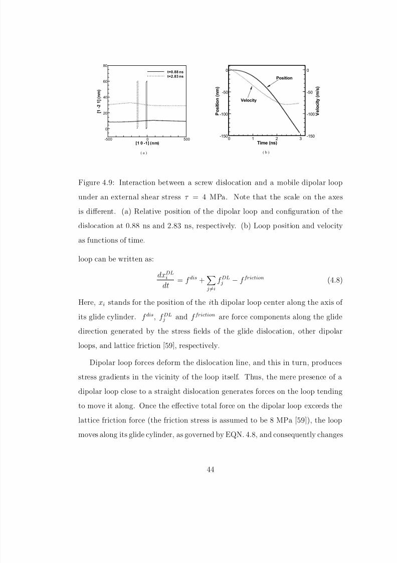
8/8/2019 Dbt Thesis Ucla
http://slidepdf.com/reader/full/dbt-thesis-ucla 63/116
[1 0 -1] (nm)
[ 1 - 2 1 ] (
n m )
-500 0 500
0
20
40
60
80
t=0.88 ns
t=2.83 ns
Time (ns)
P o s i t i o n
( n m )
0 1 2 3-150
-100
-50
0
V e l o c i t y
( m / s )
-150
-100
-50
0
Velocity
Position
(a) (b)
Figure 4.9: Interaction between a screw dislocation and a mobile dipolar loop
under an external shear stress τ = 4 MPa. Note that the scale on the axes
is different. (a) Relative position of the dipolar loop and configuration of the
dislocation at 0.88 ns and 2.83 ns, respectively. (b) Loop position and velocity
as functions of time.
loop can be written as:
dxDLi
dt= f dis +
j=i
f DL j − f friction (4.8)
Here, xi stands for the position of the ith dipolar loop center along the axis of
its glide cylinder. f dis, f DL j and f friction are force components along the glide
direction generated by the stress fields of the glide dislocation, other dipolar
loops, and lattice friction [59], respectively.
Dipolar loop forces deform the dislocation line, and this in turn, produces
stress gradients in the vicinity of the loop itself. Thus, the mere presence of a
dipolar loop close to a straight dislocation generates forces on the loop tendingto move it along. Once the effective total force on the dipolar loop exceeds the
lattice friction force (the friction stress is assumed to be 8 MPa [59]), the loop
moves along its glide cylinder, as governed by EQN. 4.8, and consequently changes
44
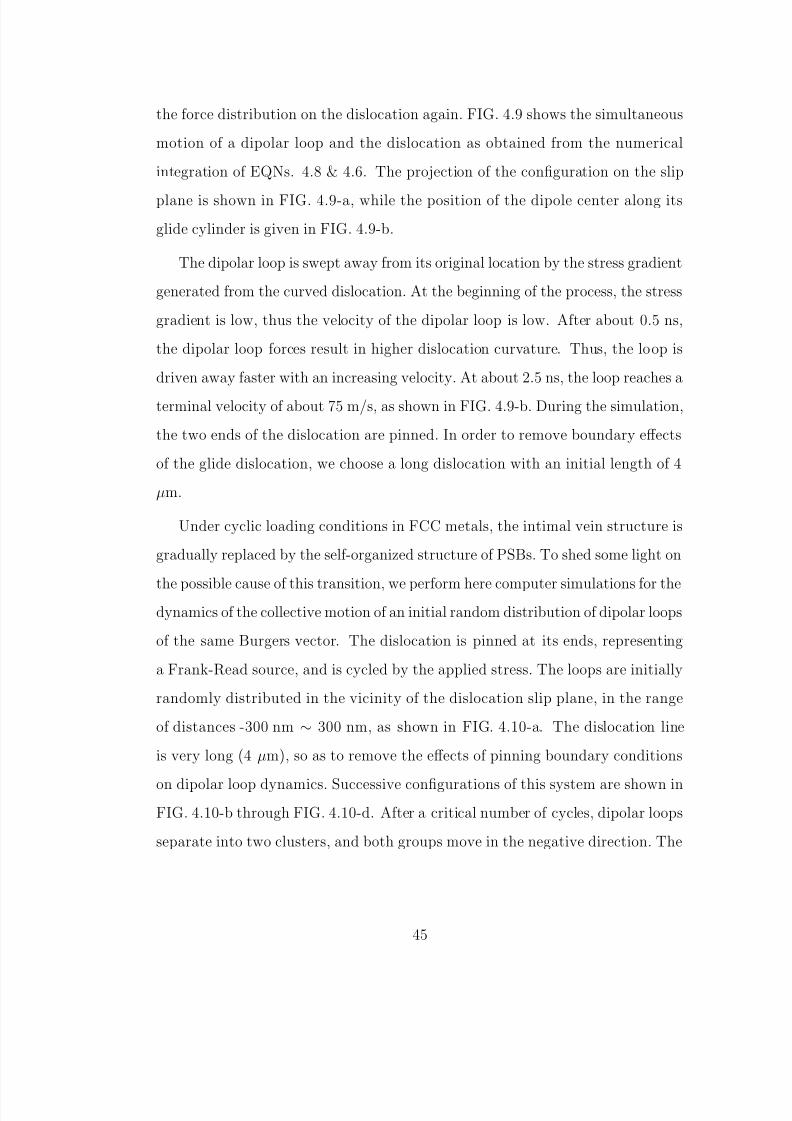
8/8/2019 Dbt Thesis Ucla
http://slidepdf.com/reader/full/dbt-thesis-ucla 64/116
the force distribution on the dislocation again. FIG. 4.9 shows the simultaneous
motion of a dipolar loop and the dislocation as obtained from the numerical
integration of EQNs. 4.8 & 4.6. The projection of the configuration on the slip
plane is shown in FIG. 4.9-a, while the position of the dipole center along its
glide cylinder is given in FIG. 4.9-b.
The dipolar loop is swept away from its original location by the stress gradient
generated from the curved dislocation. At the beginning of the process, the stress
gradient is low, thus the velocity of the dipolar loop is low. After about 0.5 ns,
the dipolar loop forces result in higher dislocation curvature. Thus, the loop is
driven away faster with an increasing velocity. At about 2.5 ns, the loop reaches a
terminal velocity of about 75 m/s, as shown in FIG. 4.9-b. During the simulation,
the two ends of the dislocation are pinned. In order to remove boundary effects
of the glide dislocation, we choose a long dislocation with an initial length of 4
µm.
Under cyclic loading conditions in FCC metals, the intimal vein structure is
gradually replaced by the self-organized structure of PSBs. To shed some light on
the possible cause of this transition, we perform here computer simulations for thedynamics of the collective motion of an initial random distribution of dipolar loops
of the same Burgers vector. The dislocation is pinned at its ends, representing
a Frank-Read source, and is cycled by the applied stress. The loops are initially
randomly distributed in the vicinity of the dislocation slip plane, in the range
of distances -300 nm ∼ 300 nm, as shown in FIG. 4.10-a. The dislocation line
is very long (4 µm), so as to remove the effects of pinning boundary conditions
on dipolar loop dynamics. Successive configurations of this system are shown in
FIG. 4.10-b through FIG. 4.10-d. After a critical number of cycles, dipolar loops
separate into two clusters, and both groups move in the negative direction. The
45

8/8/2019 Dbt Thesis Ucla
http://slidepdf.com/reader/full/dbt-thesis-ucla 65/116
[ 1 0 -1 ] (n m )
-500
0
500
[ 1 - 2
1 ]
( n m
)
0
50
100
[ 1 1 1 ] ( n
m )
0
50
100
X
Y
Z
[ 1 0 -1 ] (n m )
-500
0
500
[ 1 - 2
1 ]
( n m
)
0
50
100
[ 1 1 1 ] ( n
m )
0
50
100
X
Y
Z
[ 1 0 -1 ] (n m )
-500
0
500
[ 1 - 2
1 ]
( n m )
0
50
100
[ 1 1 1 ] ( n
m )
0
50
100
X
Y
Z
[ 1 0 -1 ] (n m )
-500
0
500
[ 1 - 2
1 ]
( n m )
0
50
100
[ 1 1 1 ] ( n
m )
0
50
100
X
Y
Z
(a) (b)
(c)(d)
Figure 4.10: The relative configuration of 20 dipolar loops at the end of different
cycles: (a)-initial, (b)-5th cycle, (c)-10th cycle, (d)-15th cycle
46
8/8/2019 Dbt Thesis Ucla
http://slidepdf.com/reader/full/dbt-thesis-ucla 66/116
8/8/2019 Dbt Thesis Ucla
http://slidepdf.com/reader/full/dbt-thesis-ucla 67/116
Similar as EQN. 4.3, the variational form of EQN. 3.2 in three dimensional
form can be written as
Γv
−A τ
τ 0m(T )
exp−Qdis
kBT n dΓ = 0 (4.9)
Here, the integration is along the dislocation line Γ, n is the unit normal vector
of the glide plane. The shear force τ is defined as τ = f g/b, f g is glide part of
the resultant line force, and b is the length of Burgers vector. With the same
discretization method, similar governing equation as EQN. 4.6 can be obtained.
The time integration scheme is the same as that of previous part.
48

8/8/2019 Dbt Thesis Ucla
http://slidepdf.com/reader/full/dbt-thesis-ucla 68/116
CHAPTER 5
Three Dimensional Crack Simulation with
Discrete Dislocation Representation Method
The distribution method originated in the investigation of the similarities of the
crack and groups of pileup dislocation. Using classical orthogonal polynomi-
als, Eshelby, et.al. studied the distribution of discrete dislocation pileups under
external loading [25]. Under simple loading condition, they obtained the distri-
bution function of the dislocations, and compared the stress field due to these
dislocations with that of a crack with freely slipping surface, the same type of
relationship of stress .vs. distance to the tip as in the crack are obtained. Later,
Leibfried [62] introduced a concept of continuous distribution dislocation to avoid
solving complicate discrete distribution function. In his method, the slip plane issupposed to contain a smeared-out sheet of dislocation density, with an amount
of bf (x)dx of Burgers vector between x and x + dx, where x stands for the posi-
tion in crack surface in 2-D. Thus the problem is converted to solve the following
singular integral type equation:
P
∞ −∞
f (x)dx
x
−x
= F (x) (5.1)
Here, P and F (x) is determined by the boundary condition and applied load.
Friedel[28, 29] is the first one who introduced the continuous distribution of
freely climbing crack dislocations to describe a crack with normal displacement
49

8/8/2019 Dbt Thesis Ucla
http://slidepdf.com/reader/full/dbt-thesis-ucla 69/116
discontinuity. Bibly and Eshelby [4] pointed out that unlike the crystal dislo-
cation, the crack dislocation is the natural discontinuities across the unwelded
cuts when a body is stressed, while in the crystal dislocation, the cuts are being
subsequently rewelded.
With the 2D continuous distribution method, the crack problems in elastic-
plastic solid has been well solved analytically [61, 88], where the complicate situa-
tion of the image stress calculation have been avoided. But due to the complicate
loading condition, the crack can not be treated in 2D. A 3D technique closely
related to the eigenstrain method is developed by Mura [68], which itself based
on earlier work of Eshelby [24] in solving ellipsoidal inclusion problem. In this
method, the 3D crack plane are assumed to be filled with infinitesimal dislocation
loops but with different densities everywhere. The stress field of this infinitesimal
loop can be obtained analytically[12, 69], by solving the similar type equations
as EQN. 5.1 but with hyper-singularity:
∞ −∞
f (x, y)dS
r3= σ0(x, y) (5.2)
Here, r =
(x − x)2 + (y − y)2 and, S is crack surface, σ0(x, y) is a known
function related to load and boundary condition.
5.1 Discrete Model in 3D cracks
In stead of solving EQN.5.2 which needs FEM method or other complicate
technique[92], we here propose another discrete method based on Parametric
Dislocation Dynamics.
According to Bueckner’s Principle [11], the stress state around a general
3-D crack in an elastic body subjected to general external loading is identical to
50
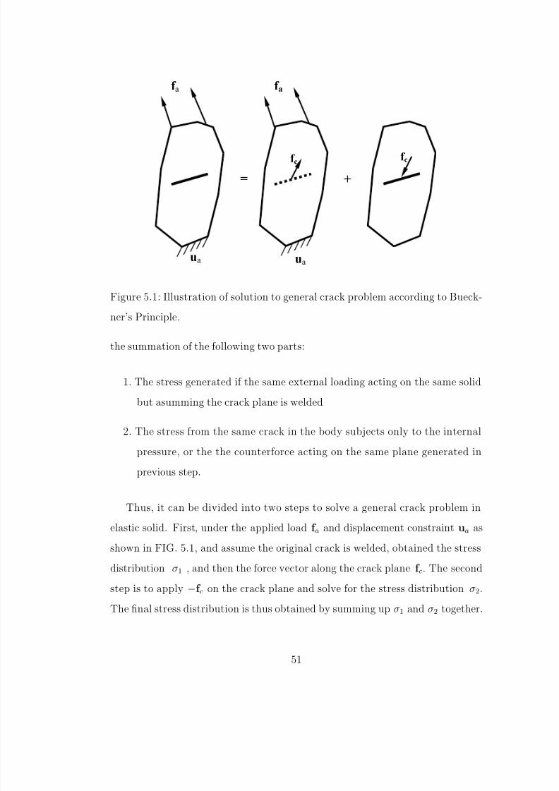
8/8/2019 Dbt Thesis Ucla
http://slidepdf.com/reader/full/dbt-thesis-ucla 70/116
ua ua
f a
=
f a
+
f c f c
Figure 5.1: Illustration of solution to general crack problem according to Bueck-
ner’s Principle.
the summation of the following two parts:
1. The stress generated if the same external loading acting on the same solid
but asumming the crack plane is welded
2. The stress from the same crack in the body subjects only to the internal
pressure, or the the counterforce acting on the same plane generated in
previous step.
Thus, it can be divided into two steps to solve a general crack problem in
elastic solid. First, under the applied load f a and displacement constraint ua as
shown in FIG. 5.1, and assume the original crack is welded, obtained the stress
distribution σ1 , and then the force vector along the crack plane f c. The second
step is to apply −f c on the crack plane and solve for the stress distribution σ2.
The final stress distribution is thus obtained by summing up σ1 and σ2 together.
51
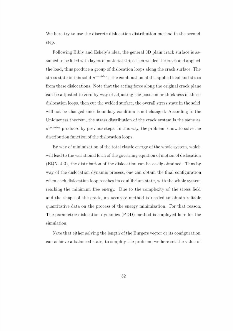
8/8/2019 Dbt Thesis Ucla
http://slidepdf.com/reader/full/dbt-thesis-ucla 71/116
We here try to use the discrete dislocation distribution method in the second
step.
Following Bibly and Eshely’s idea, the general 3D plain crack surface is as-
sumed to be filled with layers of material strips then welded the crack and applied
the load, thus produce a group of dislocation loops along the crack surface. The
stress state in this solid σcombineis the combination of the applied load and stress
from these dislocations. Note that the acting force along the original crack plane
can be adjusted to zero by way of adjusting the position or thickness of these
dislocation loops, then cut the welded surface, the overall stress state in the solid
will not be changed since boundary condition is not changed. According to the
Uniqueness theorem, the stress distribution of the crack system is the same as
σcombine produced by previous steps. In this way, the problem is now to solve the
distribution function of the dislocation loops.
By way of minimization of the total elastic energy of the whole system, which
will lead to the variational form of the governing equation of motion of dislocation
(EQN. 4.3), the distribution of the dislocation can be easily obtained. Thus by
way of the dislocation dynamic process, one can obtain the final configurationwhen each dislocation loop reaches its equilibrium state, with the whole system
reaching the minimum free energy. Due to the complexity of the stress field
and the shape of the crack, an accurate method is needed to obtain reliable
quantitative data on the process of the energy minimization. For that reason,
The parametric dislocation dynamics (PDD) method is employed here for the
simulation.
Note that either solving the length of the Burgers vector or its configuration
can achieve a balanced state, to simplify the problem, we here set the value of
52

8/8/2019 Dbt Thesis Ucla
http://slidepdf.com/reader/full/dbt-thesis-ucla 72/116
the Burgers vector b of the moving dislocation as:
b = αf c (5.3)
Here, α is a constant related to the selection of the length of the Burgers vector.
f c is the force acting on the crack plane as defined in FIG. 5.1. It is interestingly
to point out that f c is not uniform in the crack plane especially in general 3-D
loading, hence the crack dislocations in generally is of Somigliana type.
we here provide a dynamic adding-deletion strategy for the simulation to
obtain the final distribution of the dislocation, it is summarized as follows:
For a given crack, an initial distribution of 3 equally separated dislocation
loops are put on the crack plane. The shape is chosen according to the crack plane
shape with the outermost one chosen as the crack surface boundary and fixed
during the whole simulation (Here we assume there is no crack propagation.).
Under the combined effect of their mutual interactions, stress from the applied
load and their self-force, the crack dislocations will either move stretch toward
the outermost one if the effect of the applied load is dominant, or shrink if its
self-force is dominant, until reach equilibrium state. In the simulation process,
new loops are continuously adding to the simulation, and old collapsed ones are
taken out of the simulation, the strategy is:
Adding: In the adjusting process, once the innermost loop expands when the
repulsive force from other loops is less than the applied load, its charac-
teristic length r will be larger than a critical value r0, a fresh new loop is
generated in the center. r0 can be given by the equilibrium position of the
loop under the applied load and self-force, or a very small set value. Thenew loop have the same property as the old one, except its Burgers vector
is chosen, locally by EQN. 5.3. The total number of crack dislocations is
increased by one.
53

8/8/2019 Dbt Thesis Ucla
http://slidepdf.com/reader/full/dbt-thesis-ucla 73/116
Deletion: The repulsive force to the innermost loop is too large, making its
characteristic length r smaller than r0. Notice that in this case its self-force
makes the loop contract, or r smaller, and finally to zero. This loop needs
be taken out from calculation. Thus, the total number of crack dislocation
in the crack plane is decreased by one.
By way of this dynamic adding-deletion process, a final equilibrium distribu-
tion of dislocation loops can be obtained easily.
5.2 Numerical Simulation of General 3-D Crack
We analyze here the stress field of different shape of cracks under either mode-I
or mode-II load, and check the numerical precision of the distribution method.
5.2.1 Penny-shaped crack
Stress distribution in an infinite solid containing a penny-shaped crack under
arbitrary loading has been extensively studied past. Sack [76] and Sneddon [83]
first solve the problem of penny-shaped crack opened by pressure applied over
its surface in an infinite elastic solid. Collins [16] later investigated further on
the stress distribution of penny-shaped crack in thick plate. Kassir and Sih
[52] studied elliptical crack under arbitrary loading, and compare the results of
stress intensity factor under shear loading with different loading directions. A
comparison between the dislocation distribution method and analytical method
will be given below.
54

8/8/2019 Dbt Thesis Ucla
http://slidepdf.com/reader/full/dbt-thesis-ucla 74/116
5.2.1.1 Pure shearing
Considering a penny-shaped crack with diameter of 2 r0 as shown in FIG. 5.2a,
under constant pure shear loading along σxz = τ . We constructed the local coor-
dinate system on the crack plane as shown in the figure. An initial distribution
of dislocation is put inside the crack surface with 3 equally spaced circular dis-
location loops, including the outermost static one which prevents all the others
moving outside. The applied load generates a uniform shear stress field σxz.
According to EQN.5.3, the Burgers vector can be chosen as:
b = bi
Here, b is a constant number since τ is constant.
(b)(a)
Figure 5.2: Distribution of crack dislocation loops of penny penny-shaped crack
under mode-II loading with σxz = 200 MPa. (a) illustration of local coordinate
system. (b) Final distribution of crack dislocations.
FIG. 5.2b illustrates the final equilibrium distribution of crack dislocations
55

8/8/2019 Dbt Thesis Ucla
http://slidepdf.com/reader/full/dbt-thesis-ucla 75/116
under the applied shear load τ = 200 MPa. In the simulation, the constant b
is chosen as 0.4 a, the shear modulus µ = 50 GPa, Poisson’s ratio ν = 0.31,
and crack radius r0 = 1000 lattice constant a. As shown in the figure, totally 9
dislocations are fitted in the crack plane by using adding-deletion strategy. The
energy of a screw segments is lower than that of a edge one per unit length, as
a consequence, the self-force of screw component tends to be higher or stiffer
than that of a edge one, thus the edge components tend to stretch more than
screw ones as shown in the figure, and an oval configuration is generated for each
loop. Due to the effect of the outmost circular loop, the ratio of the long to
short axis of the oval loop decreases from inner to outer, as the effect field of the
outer dislocation becomes stronger. It is shown in the figure that the minimum
distance of the two outmost loops is within 10 b, in order to capture their mutual
interaction in high precision, more Gaussian quadrature points are used in the
line integral of stress calculation.
FIG.5.3a shows the distribution of σxz as a ratio of applied shear load τ ,
when compared with the analytical solution obtained by Kassir and Sih [52], the
relative error along y-direction is shown in FIG. 5.3b . Within a small range of
distance to the tip (≈ 2 % of R0), the stress drops quickly, but after that the stress
goes to a saturated value which equals to the applied load. When the distance is
far away from the crack tip, the stress is not proportional to r−1/2 as that in two
dimensional crack. When the distance is less than 0.5% of r0, the relative error
is larger than 10%. The main error comes from the the Fast Sum Method which
is used in the stress calculation. As mentioned in [39], the relative error of stress
tends to be higher when the field point is approaching the dislocation loop. Moresegments or Gaussian quadrature points are needed for higher precision. In our
simulation, when the distance is extremely small (i.e. within a distance of 0.5 %
of the radius to the crack tip), the error is inevitably high, since only 16 points
56
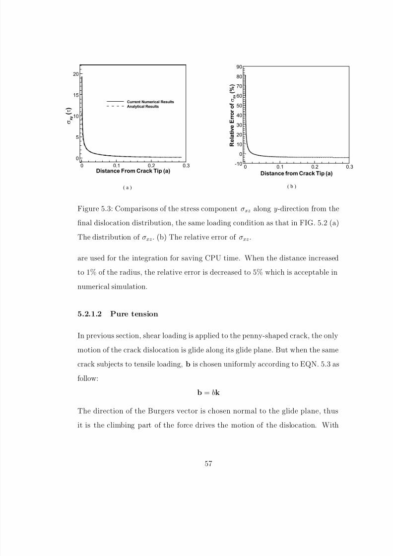
8/8/2019 Dbt Thesis Ucla
http://slidepdf.com/reader/full/dbt-thesis-ucla 76/116
Distance From Crack Tip (a)
s x y
( t )
0 0.1 0.2 0.3
0
5
10
15
20
Current Numerical Results
Analytical Results
Distance from Crack Tip (a)
R e l a t i v e E r r o r o f s z x
( % )
0 0.1 0.2 0.3-10
0
10
20
30
40
50
60
70
80
90
(a) (b)
Figure 5.3: Comparisons of the stress component σxz along y -direction from the
final dislocation distribution, the same loading condition as that in FIG. 5.2 (a)
The distribution of σxz. (b) The relative error of σxz.
are used for the integration for saving CPU time. When the distance increased
to 1% of the radius, the relative error is decreased to 5% which is acceptable in
numerical simulation.
5.2.1.2 Pure tension
In previous section, shear loading is applied to the penny-shaped crack, the only
motion of the crack dislocation is glide along its glide plane. But when the same
crack subjects to tensile loading, b is chosen uniformly according to EQN. 5.3 as
follow:
b = bk
The direction of the Burgers vector is chosen normal to the glide plane, thus
it is the climbing part of the force drives the motion of the dislocation. With
57
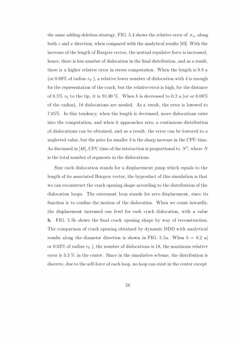
8/8/2019 Dbt Thesis Ucla
http://slidepdf.com/reader/full/dbt-thesis-ucla 77/116
the same adding-deletion strategy, FIG. 5.4 shows the relative error of σzz along
both z and x direction, when compared with the analytical results [83]. With the
increase of the length of Burgers vector, the mutual repulsive force is increased,
hence, there is less number of dislocation in the final distribution, and as a result,
there is a higher relative error in stress computation. When the length is 0.8 a
(or 0.08% of radius r0 ), a relative lower number of dislocation with 4 is enough
for the representation of the crack, but the relative error is high, for the distance
of 0.5% r0 to the tip, it is 91.00 %. When b is decreased to 0.2 a (or or 0.08%
of the radius), 18 dislocations are needed. As a result, the error is lowered to
7.65%. In this tendency, when the length is decreased, more dislocations enter
into the computation, and when it approaches zero, a continuous distribution
of dislocations can be obtained, and as a result, the error can be lowered to a
neglected value, but the price for smaller b is the sharp increase in the CPU time.
As discussed in [48], CPU time of the interaction is proportional to N 2, where N
is the total number of segments in the dislocations.
Sine each dislocation stands for a displacement jump which equals to the
length of its associated Burgers vector, the byproduct of this simulation is that
we can reconstruct the crack opening shape according to the distribution of the
dislocation loops. The outermost loop stands for zero displacement, since its
function is to confine the motion of the dislocation. When we count inwardly,
the displacement increased one level for each crack dislocation, with a value
b. FIG. 5.5b shows the final crack opening shape by way of reconstruction.
The comparison of crack opening obtained by dynamic DDD with analytical
results along the diameter direction is shown in FIG. 5.5a. When b = 0.2 a(or 0.02% of radius r0 ), the number of dislocations is 18, the maximum relative
error is 3.3 % in the center. Since in the simulation scheme, the distribution is
discrete, due to the self-force of each loop, no loop can exist in the center except
58

8/8/2019 Dbt Thesis Ucla
http://slidepdf.com/reader/full/dbt-thesis-ucla 78/116
(a) (b)
Distance to the Tip (a)
R e l a t i v e E r r o r
( % )
0 0.25 0.5 0.75 1
0
5
10
15
20
25
30
b=0.8, n=4
b=0.6, n=6b=0.4, n=9b=0.3, n=12
b=0.2, n=18
Distance to the Center (a)
R e l a t i v e E r r o r
( % )
0 0.25 0.5 0.75 1-40
-30
-20
-10
0
10
b=0.8, n=4
b=0.6, n=6b=0.4, n=9b=0.3, n=12
b=0.2, n=18
Figure 5.4: Comparisons of relative error of σzz for penny-shaped crack under
external load σzz = 200 MPa. (a) along radial direction, (b) along the vertical
direction from the center
when the length of Burgers vector is chosen as zero, which means the continuous
distribution. But with the decreasing of b, the maximum relative error for crack
opening displacement(COD) can be decreased to an acceptable level, and the
crack shape is more like an ellipsoid. That’s the why it is flat in the center shown
in FIG. 5.5b.
5.2.2 Effect of Non-uniform Stress
When there are non-uniform applied stress directly acting on the surface of the
same penny-shaped crack as that in FIG. 5.4, the shape can no longer preserve
an ellipsoid configuration. Both FIG. 5.6 and FIG. 5.7 show the different crack
shape recovered from the 3D DDD calculation. An decreasing pressure from the
center is applied along radial direction as shown in FIG. 5.6a, the pressure is
59

8/8/2019 Dbt Thesis Ucla
http://slidepdf.com/reader/full/dbt-thesis-ucla 79/116
(a) (b)
Radius (a)
C r a c k O p e n i n g ( a )
-1 -0.5 0 0.5 10
0.0005
0.001
0.0015
0.002
0.0025
Numerical Result (n=18)
Analytical Result
Figure 5.5: Comparisons of crack opening displacement(COD) with the same
condition as in FIG. 5.4 except the density of crack dislocation n=18. (a) The
COD along diameter. (b) Recover of the crack opening shape in three dimension.
chosen as
σ = pr0r
where p is a constant value, r is the distance to the center. r0 is the crack radius.To avoid singularity in the center, a cut-off distance of 0.2 r0 is chosen here. And
an increasing pressure
σ = pr
r0
is applied in FIG.5.7. In these two cases, the Burgers vector of each crack disloca-
tion is different, and changes according to its position. Since a higher pressure is
applied in the center, the center part of the crack penning shape is more obtrude
as shown in FIG. 5.6, and more flat with a lower stress as shown in FIG. 5.7
60

8/8/2019 Dbt Thesis Ucla
http://slidepdf.com/reader/full/dbt-thesis-ucla 80/116
1
5
10.2
σ ( p)
r (r 0)
r
r p
0=σ
X Y
Z
( a ) ( b )
Figure 5.6: The same penny-shaped crack as in FIG. 5.4 subjects to pressure
inside crack surface with a decreasing gradient. (a) the applied stress. (b) crack
opening shape
5.2.3 2-D straight crack
Two dimensional cracks has been extensively used in Ductile-to-Brittle transition
simulation, hence it is more important to obtain the crack dislocation distribution
under different loading condition. Notice that once the ratio of crack length to
its width is very larger, stress field of its center part can be viewed as that of a
2-D crack, hence we will try to use the same method to simulate a 2D crack.
5.2.3.1 Simple loading
Considerer a straight crack with a length 2r0
in x-direction, but with finite width
20r0 in y-direction. The normal of the crack plane is chosen along z-direction as
illustrated in FIG. 5.8a.
61
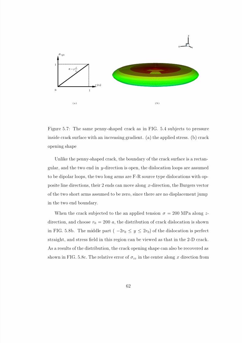
8/8/2019 Dbt Thesis Ucla
http://slidepdf.com/reader/full/dbt-thesis-ucla 81/116
XY
Z
( a ) ( b )
0
1
1
σ ( p)
r (r 0)
0r
r p=σ
Figure 5.7: The same penny-shaped crack as in FIG. 5.4 subjects to pressure
inside crack surface with an increasing gradient. (a) the applied stress. (b) crack
opening shape
Unlike the penny-shaped crack, the boundary of the crack surface is a rectan-
gular, and the two end in y-direction is open, the dislocation loops are assumed
to be dipolar loops, the two long arms are F-R source type dislocations with op-
posite line directions, their 2 ends can move along x-direction, the Burgers vector
of the two short arms assumed to be zero, since there are no displacement jump
in the two end boundary.
When the crack subjected to the an applied tension σ = 200 MPa along z-
direction, and choose r0 = 200 a, the distribution of crack dislocation is shown
in FIG. 5.8b. The middle part ( −2r0 ≤ y ≤ 2r0) of the dislocation is perfect
straight, and stress field in this region can be viewed as that in the 2-D crack.As a results of the distribution, the crack opening shape can also be recovered as
shown in FIG. 5.8c. The relative error of σzz in the center along x direction from
62
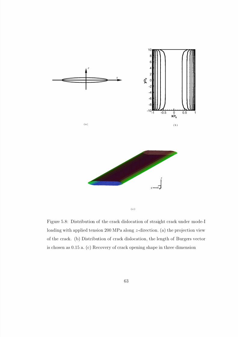
8/8/2019 Dbt Thesis Ucla
http://slidepdf.com/reader/full/dbt-thesis-ucla 82/116
X
Z
Y
z
x
( a ) ( b )
( c )
x/r 0
y / r 0
-1 -0.5 0 0.5 1-10
-8
-6
-4
-2
0
2
4
6
8
10
Figure 5.8: Distribution of the crack dislocation of straight crack under mode-I
loading with applied tension 200 MPa along z-direction. (a) the projection view
of the crack. (b) Distribution of crack dislocation, the length of Burgers vector
is chosen as 0.15 a. (c) Recovery of crack opening shape in three dimension
63

8/8/2019 Dbt Thesis Ucla
http://slidepdf.com/reader/full/dbt-thesis-ucla 83/116
the crack tip is shown in FIG. 5.9. With the increase of number of dislocation
pairs, the relative error drops significantly. With only 7 dipolar loop, the relative
error is less than 2 % when the distance is larger than 5 a (or 2.5 % r0).
Distance from Crack Tip d/r 0
R
e l a t i v e E r r o r o f σ z z
( % )
0 0.2 0.4 0.6 0.8 1
0
10
20
30
40
50
b=0.4, n=3
b=0.3, n=4
b=0.2, n=6
b=0.16, n=7
Figure 5.9: Comparison of relative error of σzz . The same condition as in FIG.
5.8
5.2.3.2 Mixed mode
When the same crack subjects to mixed mode I & II loading, the results is shown
in FIG. 5.8a. The applied tension is chosen as 200 MPa, and shear stress 100 MPa,
thus the stress tensor on crack surface is:
σ =
0 0 100
0 0 0
100 0 200
(MPa)
64

8/8/2019 Dbt Thesis Ucla
http://slidepdf.com/reader/full/dbt-thesis-ucla 84/116
thus the Burgers vector of each crack dislocation is of the form:
b =
0.05
0
0.1
a
The burgers vector has both in-plane and out-of-plane component, thus the mo-
tion of the dislocation is the mixture of climbing and gliding.
x/r 0
y / r
0
-1 -0.5 0 0.5 1-10
-8
-6
-4
-2
0
2
4
6
8
10
Horizontal Distance to the Tip d/r 0
R e l a t i v e E r r o r o
f σ z x
( % )
0 0.05 0.1 0.15 0.2 0.25
-30
-20
-10
0
10
α=45o
α=30o
α=15o
α=0o
( a ) ( b )
Figure 5.10: Straight crack under mixed model I & II loading. (a) Crack disloca-
tion distribution. (b) Comparison of relative error of σzx with different inclination
angle.
The final distribution of crack dislocation is shown in FIG. 5.10a, there are
totally 11 crack dislocation pairs in the field. FIG. 5.10b shows the comparison
of the relative error of σxz with different inclination angle to the crack plane. As
shown in the figure, when the distance is larger than 10 a, the relative error is
decreased within 5%.
65
8/8/2019 Dbt Thesis Ucla
http://slidepdf.com/reader/full/dbt-thesis-ucla 85/116
CHAPTER 6
Dislocation Activity ahead of Crack Tip
Dislocation activity ahead of crack tip plays a dominant role in the investigating
of Ductile-to-Brittle transition effect in BCC single crystal materials. Disloca-
tions ahead of crack tip basically have two toughening effects, i.e., the shielding
and blunting effects, which essentially increased the applied load necessarily to
propagate the crack. In this chapter we will study the dynamically develop-
ment of dislocation population in the vicinity of a loaded crack tip as a aid to
understand the ductile-to-brittle transition.
6.1 Three Dimensional Elastic Dislocation Interaction with
the Crack
The free crack surface result in the additional stress (or image stress), applied
on the dislocation. On the other hand, this image stress decreases the crack
tip fracture toughness. Many analytical models have been proposed to study the
shielding of a pure edge or screw dislocation in two dimensional crack[64, 85], and
its analytical estimation of shielding effect of single dislocation (i.e. EQN. 3.10)
has been well utilized in previous 2-D simulation(e.g. [74]). Devincre and Roberts
[21] provided an estimation of the local fracuure toughness that is based purely
on the crack opening or closing stress components of the dislocation stress field
at the crack tip. In their estimation, if the crack extends into the z -direction, and
66

8/8/2019 Dbt Thesis Ucla
http://slidepdf.com/reader/full/dbt-thesis-ucla 86/116
the crack plane is the y =0 plane, the σyy component of the stress tensor causes
crack opening. Then, the local stress intensity factor is written as
ktip(z) = Kapp +N
i=1
µb
|σiyy(zz)
|sign(σi
yy(zz)) (6.1)
where N is the total number of dislocation segments and σiyy(zz) is the yy -
component of the stress field of the i -th dislocation segment at position z along
crack tip. This formula gives a crude estimation for the shielding of general 3-D
dislocation, but the effects of the crack surface changes due to the existence of
the dislocation itself is not taken into consideration. Some other methods based
on Boussinesq problem of point loading in a half space [27], or weight function
method [33, 32, 34], has been attempted, but both are painstaking and not prac-tical in the real computation.
A new method based on the 3D dislocation distribution method is proposed
here. Recall in CHAP. 5, when we solve the 3D crack problem, the external load
is the only applied stress, but when there is crystal dislocation loops inside the
material, since the nature of the stress field and the external load are the same,
it can be treated the same as the external load. The Burgers vector of crack
dislocation is thus modified as:
b = α(f a + f d) = ba + bd (6.2)
Here, f a and f d are the counterforces of force vectors generated by the applied
load and crystal dislocation respectively as described in FIG. 5.1. ba = αf a is
the contribution to the Burgers vector by the applied load, usually it is constant
on the crack surface, bd = αf d is the part contributed by the crystal dislocation,
it is usually not uniform on the crack surface, and it decreases with the increaseof the distance to the crystal dislocation. Since the stress field of the dislocation
decreases quickly, the effective area to the Burgers vector of the crack dislocation
is very small.
67
8/8/2019 Dbt Thesis Ucla
http://slidepdf.com/reader/full/dbt-thesis-ucla 87/116
With the same procedure of obtaining the final distribution as that in CHAP.
5, one can obtain the overall stress field under both the external load and the
crystal dislocations. The stress field from such a distribution can be also divided
into two parts, one is the original stress from crack under external loading, and
the other is the extra part due to the crack free surface, and this part is the
so-called image stress.
The local fracture toughness at each point along the crack tip can be easily
obtained from this stress distribution by:
K = limr→0
σ(r)√
2πr (6.3)
Thus the shielding effect of the dislocation K d can be obtained by
Kd = Ka − Kt (6.4)
Here Kt is the total toughness obtained by the crack dislocation distribution, and
Ka is the applied fracture toughness. When Kd is larger than zero, the overall
toughness is decreased, hence the dislocation has shielding effect on the crack, on
the contrary, when Kd < 0, it has anti-shielding effect to the crack.
As a comparison, we here use the 3-D model to simulate the shielding effect
of an 2D straight edge dislocations ahead of a finite slit crack, and compare that
with the analytical results obtained by Wang and Lee[85]. Suppose a finite crack
with length 2r0 = 1000 a, the width is sufficiently long of 20r0, its tip along
[010]-direction and (001)-plane as its crack plane, an straight edge dislocation
with b = 12
[101](1̄01) is introduced to the calculation. It sits on the slip plane
(¯101) with a distance d to the crack tip. Before the introduction of the edge dislo-
cation, the crack plane is already filled with equilibrium state crack dislocations
at the applied stress σ = 200 MPa. With the existence of the dislocation, the
equilibrium state is broken, the distributed dislocation will re-adjust their config-
68

8/8/2019 Dbt Thesis Ucla
http://slidepdf.com/reader/full/dbt-thesis-ucla 88/116
uration till the new equilibrium state. From this new equilibrium distribution of
crack dislocation, the image stress as well as its shielding effect can be obtained.
Relative Distance d/a
K I d
/ K I a
0.05 0.1 0.15 0.2 0.25 0.3
0.2
0.4
0.6
0.8
Analytical ResultsNumerical Results
r 0r 0
θ
b
d
σ
( a ) ( b )
Figure 6.1: Interaction of an edge dislocation and a straight crack in 2D. (a)
relative position of crack and the edge dislocation, r0 is the half width of the
crack. (b) comparison of fracture toughness with the analytical solution.
It is shown in FIG. 6.1 that with the increase of the the distance to the tip, the
shielding effect decreases, and the numerical results is about 2 times of analytical
results. This is due to the consideration of crack surface roughness generated by
the existence of the crystal dislocation, and hence the numerical results have a
higher shielding effects.
Under the same condition as in FIG. 6.1, when the straight dislocation is
replaced by a circular dislocation loop with b = 12
[101], the shielding effect is
shown in FIG. 6.2. The distance of the center of the loop to the crack tip is
chosen as 100 a. The the stress intensity factor of the loop with the change of
the radius R0 is shown in FIG. 6.2b. The contour plot of the {33 } component of
69

8/8/2019 Dbt Thesis Ucla
http://slidepdf.com/reader/full/dbt-thesis-ucla 89/116
the stress tensor of the shear loop σ33 is shown in FIG. 6.2a when R0 is chosen
as 50. σ33 is always negative, having a tendency to close the crack, thus it has a
shielding effect to the crack. When the radius is increased, the shear loop is more
close to the tip, thus it has a higher shielding effect. And since the stress field of
the loop can only affect a small area, the shielding effect is within a small zone.
The effective shielding area is within −500 a ∼ 500 a as shown in the figure
x (a)
y ( a )
-200 0 200 400-400
-300
-200
-100
0
100
200
300 σ33
(MPa)
-0.03
-0.1
-0.3
-1
-5
-20
-40
-60-80
-100
-120
-140
Position along Crack Tip (a)
K d
-500 0 500
0
0.05
0.1
0.15R
0=30 a
R0=40 a
R0=50 a
R0=60 a
)
(
m
M P a
Figure 6.2: Shielding effect of a shear dislocation loop ahead of crack tip. (a)
contour of the the the {33 } component of the stress tensor by the shear dislocation
loop. the radius R0 is 50 a. (b) comparisons of the shielding at different radius.
6.2 Motion of Dislocation ahead of Crack Tip
Dislocation motion ahead of crack tip is quite complicate, and it is a key issue to
understand the change of fracture toughness.
Suppose a straight dislocation emanated from a finite crack tip and starts
to move away from the tip, FIG.6.3 shows its configuration and corresponding
70

8/8/2019 Dbt Thesis Ucla
http://slidepdf.com/reader/full/dbt-thesis-ucla 90/116
Along crack tip (a)
N o r m a l t o c r a c k t i p ( a )
-400 -200 0 200 400
20
40
60
80
100
120
0
0.59 ms
1.12 ms
1.59 ms
2.05 ms
2.50 ms
2.95 ms
3.42 ms
3.88 ms4.35 ms
Along Crack Tip (a)
K d / K
a
-400 -200 0 200 4000
0.2
0.4
0
0.59 ms
1.12 ms
1.59 ms
( a )
( b )
Figure 6.3: Motion of dislocation half loop ahead of crack tip. The initial size of
the loop is chosen 400 a. (a) configuration of the dislocation at different time.
(b) the corresponding shielding effect of the dislocation to the crack.
71

8/8/2019 Dbt Thesis Ucla
http://slidepdf.com/reader/full/dbt-thesis-ucla 91/116
shielding effect to the crack. The size of the crack is chosen as 2r0 = 1000a,
and (100) is its crack plane. The uniaxial applied stress is σ11 = 3.0 GPa (or
Ka = σ11√
πr0 = 2.11 MPa√
m). The Burgers vector of the crystal loop is chosen
along (111̄)-direction with length 0.274 nm and its glide plane is (101) with an
angle of 45◦ to the crack plane. The length of the loop is initially chosen as 400
a with its two ends at (-200 a,15 b), (200 a,15 b) respectively. The two ends
are confined to slid along the crack tip direction. b is chosen as 0.274 nm. The
material constant m is chosen as 2, the temperature is chosen as 450 K, so the
force-velocity relation EQN. 3.2 can be rewritten as:
v = M (τ /τ 0)
2
(6.5)
Here, M is effective mobility and M = 2.47 × 10⁻³ sec/a, v is the nodal velocity.
The effect of the free surface of the crack dislocation, or the image stress tends
to pull the dislocation back to the crack, thus it has a shielding effect. In order
to avoid being totally pulled back, the initial distance of the dislocation to the
crack tip is chosen as 15 b. Under the driving force of the crack, the dislocation
starts to move away from the tip. At its early stage, when t <3.5 ms, due to the
image stress, the total stress applied on the dislocation in the center part is much
lower than that at the two ends, thus its speed is much lower, and a concave
configuration is generated. With the dislocation continually moving away from
the tip, the effect of the image stress decreases, and the concave configuration
gradually disappeared as shown in FIG. 6.3a when t=3.88 ms. After that, due
to the fast decaying of the crack stress, the speed of the nodes in the center
part is still lower than that at the two side, thus a flat roof is generated and theflat roof becomes more longer during the motion. The shielding effect Kd of the
dislocation is shown in FIG.6.3b. It initially has a maximum shielding effect of
around 50 % of Ka at the center, but after 0.59 ms, the shielding of the center
72

8/8/2019 Dbt Thesis Ucla
http://slidepdf.com/reader/full/dbt-thesis-ucla 92/116
x (a)
y
( a )
-500 0 500
50
100
150
σ11
30
25
20
15
10
8
64
2
1.5
1
x (a)
y
( a )
-500 0 500
50
100
150
σ11
30
25
20
15
10
8
64
2
1.5
1
x (a)
y
( a )
-500 0 500
50
100
150
σ11
30
25
2015
10
8
6
4
2
1.5
1
x (a)
y
( a )
-500 0 500
50
100
150
σ11
30
25
20
15
10
8
6
4
2
1.5
1
x (a)
y
( a )
-500 0 500
50
100
150
σ11
30
25
20
15
10
8
6
4
2
1.5
1
x (a)
y
( a )
-500 0 500
50
100
150
σ11
30
25
20
15
10
8
6
4
2
1.5
1
( a ) ( b )
( e )
( d )( c )
( f )
Figure 6.4: Contour of the {11} component of the stress tensor from crack tip
due to the applied stress and image stress. (a) t=0, (b) t=0.59 ms, (c) t=1.59
ms, (d) t=2.50 ms, (e) t=3.42 ms, (f) t=4.35 ms
73
8/8/2019 Dbt Thesis Ucla
http://slidepdf.com/reader/full/dbt-thesis-ucla 93/116
is only 27 % of Ka. Due to the stretch of the dislocation, the dislocation can
cover more part of the crack tip field, thus more area of the crack tip fracture
toughness is lowered. FIG. 6.4 shows the contour of {11 } component of the total
stress (original crack tip stress plus the image part) from the crack at t=0, 0.59
ms, 1.59 ms, 2.50 ms, 3.42 ms, 4.35 ms respectively. The images stress only affect
a small area near the dislocation, and it decreases the crack tip stress field. With
the increase of the distance of the dislocation to the crack tip, this effect becomes
more and more weak.
As a comparison, when the initial size of the straight dislocation is a small
value of 40 a, FIG. 6.5 shows the motion of the dislocation loop and its corre-
sponding shielding effect with a different shape. The initial effect field of the
dislocation is very narrow as can be seen from FIG.6.5b when t <0.01 ms , and
due to its two ends are confined sliding along crack tip, the concave configuration
is very small which is different from FIG. 6.3, it is very easily recovered at around
t=0.07 ms. At the time of recovery, the difference between the maximum dis-
tance at the center part and minimum distance at two sides part is only around
5 a. Thus when compared with 83 a in FIG. 6.3, variance of the nodal speed in
the dislocation is not very large, thus there is no flat roof in its configuration as
shown in FIG.6.5a, the center part starts to protrude out during the motion.
6.3 Dislocation Nucleation
In this section, we will focus on the way of the dislocation nucleation around
the three dimensional crack. Xu et. al. [90, 91] has studied the saddle-pointconfigurations of embryonic dislocation loops near crack tip and their associated
energy with a variational boundary integration method based on the continuous
distribution dislocation method. Here, we will directly assume that the nucle-
74

8/8/2019 Dbt Thesis Ucla
http://slidepdf.com/reader/full/dbt-thesis-ucla 94/116
Along crack tip (a)
D i s t a n c e t o t h e t i p ( a )
-200 -100 0 100 200
20
40
60
80
0.59 ms
1.12 ms
1.59 ms
2.05 ms
2.50 ms
2.95 ms3.42 ms
0.01 ms
Along crack tip (a)
K d / K
a
-200 -100 0 100 2000
0.1
0.2
0.3
0.01 ms
3.42 ms
( a )
( b )
Figure 6.5: Motion of dislocation half loop ahead of crack tip. The initial size of
the loop is chosen as 40 a. (a) configuration of the dislocation at different time.
(b) the corresponding shielding effect of the dislocation to the crack.
75

8/8/2019 Dbt Thesis Ucla
http://slidepdf.com/reader/full/dbt-thesis-ucla 95/116
ation of the embryonic dislocation is easy and can be nucleated immediately at
different site along the crack tip without any cost. The initial configuration of
the embryonic dislocation is assumed to be short straight dislocation segment,
and can only bow out with its two ends sliding along the direction of crack tip,
forming half loops. When the neighboring dislocation half loops meet, they will
coalesce to form a longer one and continue bowing out.
Suppose a semi-infinite crack extends along (010) direction, the crack plane
is chosen as (100). A slip plane is chosen as (101) with an angle of 45◦ to the
crack surface. The simulation temperature is chosen as 200 K, the initial applied
load is set to 1.3 MPa√
m, and the loading rate K̇ is chosen as 0.05 MPa√
m/s.
The constant m is chosen as 2. Thus the dislocation has the same stress-velocity
relation as EQN.6.5, but the constant M = 5.14 × 10⁻⁶ a/sec.
The detailed dislocation nucleation process on the slip plane from the crack
tip and the corresponding loading history is shown in FIG. 6.6 & 6.7 respectively.
The length of the straight dislocation embryonic is chosen as 20 a. In order to
avoid the complicate boundary effect, a periodic boundary condition along the
direction of the crack tip is used during the simulation, the width of the crack ischosen as 3000 a. Assume that there are five equally separated nucleation sites
with a distance of 600 a between the neighbors. Under the crack tip stress field,
the dislocation embryo begins bowing out with their two ends confined to slide
along the crack tip direction. At each time step, we will check these five sites,
once there is enough space to put a new embryo loop, a new loop is assumed
nucleated, but after this time step, due to the repulsive force of earlier nucleated
dislocations, if the new dislocation is pushed back to the tip, it will be taken
outside the simulation. FIG. 6.6 shows the successive loop nucleation process.
The loops starts to nucleate at t = 0, and after around 2.5 sec, new embryo
76
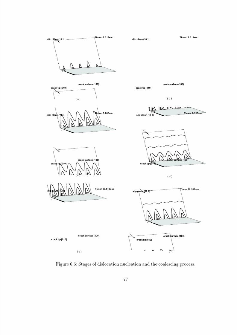
8/8/2019 Dbt Thesis Ucla
http://slidepdf.com/reader/full/dbt-thesis-ucla 96/116
slip plane (10 1)
crack tip [010]
crack surface (100)
Time= 7.518secslip plane (10 1)
crack tip [010]
crack surface (100)
Time= 2.518sec
slip plane (10 1)
crack tip [010]
crack surface (100)
Time= 8.518secslip plane (10 1)
crack tip [010]
crack surface (100)
Time= 8.268sec
slip plane (10 1)
crack tip [010]
crack surface (100)
Time= 20.518sec
(a) (b)
(c) (d)
(e) (f)
slip plane (10 1)
crack tip [010]
crack surface (100)
Time= 10.518sec
Figure 6.6: Stages of dislocation nucleation and the coalescing process.
77

8/8/2019 Dbt Thesis Ucla
http://slidepdf.com/reader/full/dbt-thesis-ucla 97/116
Time (sec)
K I
-50 0 50 1000
1
2
3
4
KApplied
KCrack tip
)
(
m
M P a
Figure 6.7: The applied and the effective fracture toughness as a function of
loading time.
loops generated at the middle three nucleation site as shown in FIG. 6.6a. After
another 5 sec, the outer dislocation loops begin meet and merge to form a longer
one as shown in FIG.6.6 (b), (c) and (d). The two ends of the longer dislocation
are still confined to slide along the crack tip direction. Once the two ends of
the longer dislocation loop reaches the crack boundary, it covers the whole crack
front, we assume they can move along the slip plane boundary, thus it moves
away from the crack as shown in FIG.6.6e when t>8.5 sec.
As discussed before, the short segments can only have shielding effects at its
nearby location, the part that not covered by the loops tends to have highest
fracture toughness, it has no contribution to the maximum fracture toughness
along the crack tip, the crack always first propagates at the site with maximumfracture toughness. We define here the effective toughness as the maximum stress
intensity along the crack tip at current time, and denoted as Ke. So the shielding
78

8/8/2019 Dbt Thesis Ucla
http://slidepdf.com/reader/full/dbt-thesis-ucla 98/116
effect of these short dislocations has no contribution to Ke, we will disregard this
shielding effect during the later calculation, and later when we mention a new
loop is nucleated means a such kind of loop is generated.
It can be shown in FIG. 6.7 that Ke is identical to the applied load Ka, until
after around 9.0 sec when the first long dislocation covers the whole crack tip,
there is a sharp drop of around 0.35 MPa√
m in Ke, that means the dislocation
has an effective shielding effect of 0.35 MPa√
m. After that, Ke increases with
the increase of the applied load. After another 5 sec, the second long dislocation
is generated, and there is a further drop in Ke of 0.42 MPa√
m. But the effective
shielding of the two dislocation is only 0.71 MPa√
m, that is because the first
dislocation moves further away from the top as shown in FIG.6.6f. Due to the
mutual interactions of the already nucleated dislocations, the time for forming a
new one is longer and longer. It takes around around 7 and 13 seconds for the
generation of the third and fourth dislocation respectively, as shown in FIG. 6.7.
All these dislocations forming a pileup on the slip plane.
The lattice resistance to the movement of the dislocation loop, the Peierls
stress, or friction stress, plays an important role in the motion of dislocation.The equation of motion EQN. 4.3 should be modified as:
v =
Aτ −τ f τ 0
m(T )exp
−Qdis
kBT
τ > τ f
0 τ ≤ τ f (6.6)
FIG. 6.8 shows the effect of the friction stress to the dislocation nucleation.
With the increase of the friction stress, the speed of generation of new loops
decreases. The maximum difference of the time for generation of the 1st loop isaround 1.82 sec, the 3rd one is around 1.94 sec, while the difference of the fifth
one is around 3.87 sec as shown in the figure. In this tendency, the time gap will
increase more and more, after a longer time, there will be a huge difference of the
79

8/8/2019 Dbt Thesis Ucla
http://slidepdf.com/reader/full/dbt-thesis-ucla 99/116
Friction Stress (MPa)
T i m e ( s e c )
0 100 200 300 4000
10
20
30
40
50
60
Figure 6.8: Time for nucleation of fresh new loops at different friction stress.
Lines count from bottom to top stands for time for the nucleation of the 1st to
5th loop
number of generated dislocations, and as a result there will be large difference of
their totally shielding effect, which will lead to the brittle-to-ductile transition.
6.4 Brittle to Ductile Transition
Dislocation velocity varies significantly at different temperature under the same
applied shear stress as shown in FIG. 6.9 (refer to EQN. 3.2). Under the applied
shear stress τ =1 and 5 GPa, the ratio of the highest and lowest velocity is about
106. The huge difference of velocity at different temperature makes it possible
for more dislocation generated at the same time interval for higher temperature,
and thus have more shielding effects on the crack tip. On the other hand, the
huge velocity difference makes the right selection of time step difficult, since
the time step should be small enough to accommodate the high speed in higher
80
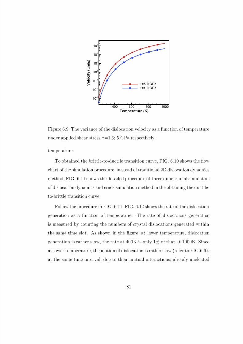
8/8/2019 Dbt Thesis Ucla
http://slidepdf.com/reader/full/dbt-thesis-ucla 100/116
Temperature (K)
V e l o c i t y ( µ m / s )
400 600 800 1000
10-3
10-2
10-1
100
101
102
103
τ=5.0 GPa
τ=1.0 GPa
Figure 6.9: The variance of the dislocation velocity as a function of temperature
under applied shear stress τ =1 & 5 GPa respectively.
temperature.
To obtained the brittle-to-ductile transition curve, FIG. 6.10 shows the flow
chart of the simulation procedure, in stead of traditional 2D dislocation dynamics
method, FIG. 6.11 shows the detailed procedure of three dimensional simulationof dislocation dynamics and crack simulation method in the obtaining the ductile-
to-brittle transition curve.
Follow the procedure in FIG. 6.11, FIG. 6.12 shows the rate of the dislocation
generation as a function of temperature. The rate of dislocations generation
is measured by counting the numbers of crystal dislocations generated within
the same time slot. As shown in the figure, at lower temperature, dislocation
generation is rather slow, the rate at 400K is only 1% of that at 1000K. Since
at lower temperature, the motion of dislocation is rather slow (refer to FIG.6.9),
at the same time interval, due to their mutual interactions, already nucleated
81
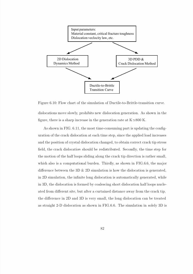
8/8/2019 Dbt Thesis Ucla
http://slidepdf.com/reader/full/dbt-thesis-ucla 101/116
Input parameters:
Material constant, critical fracture toughness
Dislocation veclocity law, etc.
3D PDD &
Crack Dislocation Method
2D Dislocation
Dynamics Method
Ductile-to-Brittle
Transition Curve
Figure 6.10: Flow chart of the simulation of Ductile-to-Brittle-transition curve.
dislocations move slowly, prohibits new dislocation generation. As shown in the
figure, there is a sharp increase in the generation rate at K800 K.
As shown in FIG. 6.11, the most time-consuming part is updating the config-
uration of the crack dislocation at each time step, since the applied load increases
and the position of crystal dislocation changed, to obtain correct crack tip stressfield, the crack dislocation should be redistributed. Secondly, the time step for
the motion of the half loops sliding along the crack tip direction is rather small,
which also is a computational burden. Thirdly, as shown in FIG.6.6, the major
difference between the 3D & 2D simulation is how the dislocation is generated,
in 2D simulation, the infinite long dislocation is automatically generated, while
in 3D, the dislocation is formed by coalescing short dislocation half loops nucle-
ated from different site, but after a curtained distance away from the crack tip,the difference in 2D and 3D is very small, the long dislocation can be treated
as straight 2-D dislocation as shown in FIG.6.6. The simulation in solely 3D is
82

8/8/2019 Dbt Thesis Ucla
http://slidepdf.com/reader/full/dbt-thesis-ucla 102/116
At each time step
Check each nucleation site
Enough Space for new half Loop?
New half loops generated
Minimum Distance of
Neighbouring half loops < critical value?
Neighbouring half loops coalease
forming a longer one
Yes
No
Yes
Yes
No
No
Start
For each temperature
Next temperature
Updating configuration of crack dislocations
only long loops have effect on the crack
Check fracture toughness along each point of the crack
Using 3D PDD updating the new configurationof each dislocation
Check the maximum speed of all the nodes
Obtaining the time step for next stepmax
V
Check each loops, remove backward moving loops
Increase applied load
Maximum K > Critical Value?
Next time step
Figure 6.11: Flow chart of the 3D simulation of PDD & crack dislocation simu-
lation.
83

8/8/2019 Dbt Thesis Ucla
http://slidepdf.com/reader/full/dbt-thesis-ucla 103/116
Temperature (K)
R a t e ( n u m / s e c )
400 600 800 10000
2
4
6
8
10
12
smK /03.0 MPa=&
smK /14.0 MPa=&
Figure 6.12: The rate of dislocation generation as a function of temperature at
different applied load.
very time consuming and is beyond the current computation limitation unless
the loading rate is artificially high, which will lead to the mistakenly shift of the
ductile-to-brittle transition[73].
As a conclusion of this part, FIG.6.13 shows the ductile-to-brittle transi-tion with 2D simulation method. The critical applied load kc when Ke reaches
the critical fracture toughness, increases as the temperature raise. As shown in
FIG.6.13a, when the temperature raised from 300 K to 1100 K, kc is raised by
a factor of 2.5. The decreasing of the loading rate also increase the overall kc as
shown in the figure. When the loading rate K̇ is decreased from 0.028 MPa√
m/s
to 0.01 MPa√
m/s, the overall kc is increased by an average of 6.0 %, which due to
the more dislocation generation, and when the loading rate is further decreasedto 0.001 MPa
√m/s, there is another 10 % increase in kc. Similar to FIG. 6.7, in
2D simulation, it is also a zigzag curve in the loading history curve as shown in
84

8/8/2019 Dbt Thesis Ucla
http://slidepdf.com/reader/full/dbt-thesis-ucla 104/116
FIG. 6.13b.
Temperature (K)
400 600 800 1000
2
3
4
KApplied
K e
0 2 4 6 80
0.5
1
1.5
2
/smMPaK 028.0=&
/smMPaK 010.0=&
/smMPaK 001.0=&
( a ) ( b )
)( mMPa
)
(
m
M P a
T=1000 K
/smMPaK 028.0=&
c r i t
c
k
K /
Figure 6.13: Relative fracture toughness as a function of temperature at different
applied load. (a) Brittle-to-Ductile transition curve at different loading rate. (b)
the loading history at T=1000 K.
85

8/8/2019 Dbt Thesis Ucla
http://slidepdf.com/reader/full/dbt-thesis-ucla 105/116
CHAPTER 7
Conclusions and Discussion
The three dimensional nature of dislocation processes ahead of crack tip is quite
complex and it is essential to understand the ductile-to-brittle transition in BCC
metals.
In current work, several topics related to dislocation theory has been fully
exploited.
7.1 Three Dimensional Parametric Dislocation Dynamics
and its Convergence and Accuracy
Based on the Fast Sum Method, the present work attempts to present a com-
prehensive investigations of the the Parametric Dislocation Dynamics Method
(PDD) as well as its fundamental mechanism in the simulation of plastic defor-
mations.
Numerical studies of dislocation generation by the Frank-Read mechanism
revealed a number of significant features. The shape accuracy of an simple equi-
librium F-R source has been shown to be excellent with only a few parametric
segments, with only two segments, a maximum relative accuracy of 10−3
can be
achieved. For complicate unstable F-R source, it requires more segments, and six
segments produce similar accuracy. The shapes of both equilibrium and unstable
86
8/8/2019 Dbt Thesis Ucla
http://slidepdf.com/reader/full/dbt-thesis-ucla 106/116
F-R sources were shown to be absolutely converge with the increase of the num-
ber of segments. Adaptive node re-distribution and a higher nodal density on the
dislocation line regions with high curvature is necessary for the annihilation event
and the subsequent loop reconfiguration. The selection of implicit and explicit
integration scheme of the system equation of motion EQN. 4.6 should take more
consideration. The numerical stability for the implicit one can be always being
assured, while for the same numerical stability, the time step should be reduced
to less than less than 500 dimensionless units (on the order of 1 ps for a mobility
of 104Pa−1s−1).
In the case of a finite size dipole, with only 2 segments on each dislocation, the
formation and destruction dynamics are resolved with a relative accuracy of less
than 10−2. The formation dynamics reveals that the two interacting dislocations
do not feel one another till their closest segments are within ≈ 100 a. It is found
that the stress to unzip the dipole is smaller than the breakup stress of finite size
dipoles, nearly by a factor of 2. On the other hand, to break up the dipole by
pushing the two dislocations past one another (forward destruction) requires a
stress that is nearly 30% higher than the infinite dipole.
Studies of the process of unstressed sessile junction formation with PDD, and
its destruction by an externally applied stress has been consistent with similar
recent studies with other methods. However, less number of required segments
for each dislocation is required for spatial resolution of less than 10−3, and for
temporal resolution of 10−6.
Its also shown that PDD is also a convenient tool for studies of elementary
mechanisms of dislocation pattering caused by elastic interactions amongst de-
fects. The method is accurate enough to deal with complex stress fields associated
with the dynamic motion of dipolar dislocation loops and glide dislocations. The
87

8/8/2019 Dbt Thesis Ucla
http://slidepdf.com/reader/full/dbt-thesis-ucla 107/116
present investigation has demonstrated a number of physical processes involved
in the sweeping mechanism.
7.2 Three Dimensional Crack Simulation
Two dimensional continuous dislocation distribution method has been extensively
studied analytically and numerically by previous work[88, 61, 50]. In the contin-
uous method, the cracks are assumed to be a distribution of loops with infinites-
imal length of Burgers vector, and by way of solving a complicated singular (in
2D) or hyper-singular (in 3D) integral equations, one can obtain its distribution
function. In this work, we assume that the crack surface is filled with discrete
dislocation loops with finite burgers vector. By way of minimization of system
free Gibbs energy, PDD is utilized to obtain the final equilibrium distribution and
configuration of these dislocation loops under the applied load. The stress field
from these distributions is the right answer to the original crack tip field. The
outer dislocation of the distribution is assumed to be the contour of the crack
surface and being fixed, the rest dislocation loops can be obtained by a dynamic
adding-deletion process. The crack opening displacement can be easily obtained
from the distribution since each dislocation loop stands for one layer of displace-
ment jump, and hence the crack opening shape can also be easily reconstructed.
It is shown that high accuracy can be obtained in the mode I & II loading in
penney-shaped and slit crack. The relative error of the stress field tends to be
higher when the field point is near to the crack tip, and more nodal points and
Gaussian Quadrature points are needed for the same accuracy. The Burgers vec-
tor is chosen as proportional to the applied load, such that the changes of the
applied load will not changes the dislocation distribution significantly.
88

8/8/2019 Dbt Thesis Ucla
http://slidepdf.com/reader/full/dbt-thesis-ucla 108/116
7.3 Crack-Dislocations Interactions as well as Ductile-to-
Brittle Transition
It is easy to derive a closed formulation for the stress field of a dislocation ahead of
of semi-infinite crack in two dimensional, but similar formulation for an arbitrary
oriented dislocation loops ahead of the crack tip is beyond the state of the art.
Three Dimensional Discrete Dislocation Distribution(DDD) provide us a useful
tool to investigate the interactions of crack and dislocation in 3D space. In
current work, the stress field of the crystal dislocation can be treated the same
as the applied load. Thus modify the equation of Burgers vector, and add the
contribution part from the stress field of the crystal dislocation, then rearrange
the configuration of the dislocations, one can obtained the changes of the crack
tip field due to the existence of crystal dislocations and change of the applied
load. As a result of the redistribution, the shielding effect of the dislocation can
be obtained.
The motion of dislocation ahead of crack tip is rather complicated. The
motion of the dislocation changes its shielding effects to the crack tip, and on
the other hand, the changed crack tip field will changes the motion speed of
the dislocation. It is shown that different initial size has different behavior of
motion, since the crack free surface has a different feedback to the motion of
the dislocation. The concave configuration due to the dragging effect of the
image stress can be easily recovered when the initial length is short. In the
simulation, it is assumed that embryonic dislocation can be generated at separate
nucleation site instantly and without any cost. The embryonic dislocation willbow out and once the neighboring dislocation loops meet, they will coalesce
and form a longer one, until cover the whole crack front. We assume that only
those dislocation covering the whole crack tip has a shielding effect to the crack,
89

8/8/2019 Dbt Thesis Ucla
http://slidepdf.com/reader/full/dbt-thesis-ucla 109/116
since those short dislocation half loops only have local shielding effect. It is
found that the major difference between the 3D and 2D simulation is how the
dislocation is nucleated, but it is still important in the understanding of ductile-
to-brittle transition behavior, especially when we need to take the friction stress,
and other type of material defects into consideration, but we should pay the price
for extensive computational time.
90

8/8/2019 Dbt Thesis Ucla
http://slidepdf.com/reader/full/dbt-thesis-ucla 110/116
References
[1] A.S. Argon and B.J. Gally. Selection of crack-tip slip systems in the thermalarrest of cleagage cracks in dislocation-free silicon single crystals. Scripta
Materialia , 45:1287–1294, 2001.
[2] R.W. Armstrong. Cleavage crack propagation within crystals by the griffithmechanism .vs. a dislocation mechanism. Mater. Sci. Engng., 1:251, 1966.
[3] G. Bergmann and H. Vehoff. Effect of environment on the brittle to ductiletransition of precracked nial single and polycrystals. Mat. Sci. & Eng. A,193:309–315, 1995.
[4] B.A. Bibly and J.D. Eshelby. Dislocation and the theory of fracture. Frac-ture, pages 99–182, 1968.
[5] B.A. Bilby, A.H. Cottrell, and K.H. Swinden. The spread of plastic yieldfrom a notch. Proc. Roy. Soc. Ser A, 272:304–314, 1963.
[6] A.S. Booth. The brittle-ductile transition in γ -TiAl . PhD thesis, Universityof Oxford, 1994.
[7] A.S. Booth and S.G. Roberts. Warm-prestressing and slow crack growth inmgo. J. Am. Ceram. Soc., 77:1457–1466, 1994.
[8] M. Brede and P. Haasen. The brittle-to-ductile transition in doped siliconas a model substance. Acta Metallurgica , 36:2003–2018, 1988.
[9] M. Brede, K.J. Hsia, and A.S. Argon. J. Appl. Phys., 70:758, 1991.
[10] L.M. Brown. Phil. Mag., 15:363, 1967.
[11] H.F. Bueckner. The propagation of cracks and the energy of elastic defor-mation. J. Appl. Mech., pages 1225–1230, 1958.
[12] J.M. Burgers. Some consideration on the field of stress connected with dis-locations in a regular crystal lattice. Proc. K. Ned. Akad., 42:293–324, 1939.
[13] G. Canova, Y. Brechet, and L. P. Kubin. 3D dislocation simulation of plastic
instabilities by work-softening in alloys. RIS∅ National Laboratory, Roskilde,Denmark, 1992.
[14] G. Canova, Y. Brechet, L.P. Kubin, B. Devincre, V. Pontikis, and M. Con-dat. 3D Simulation of dislocation motion on a lattice: application to theyield surface of single crystals. CH-Transtech, 1993.
91

8/8/2019 Dbt Thesis Ucla
http://slidepdf.com/reader/full/dbt-thesis-ucla 111/116
[15] Y.-H. Chiao and D.R. Clarke. Acta Metall., 37:203, 1987.
[16] W.D. Collins. Some axially symmetric stress distributions in elastic solidscontainning penny-shaped cracks. i. cracks in an infinite solid and a thickplate. Proc. Roy. Soc., 266:359–386, 1962.
[17] B. Devincre. Meso-scale Simulation of the Dislocation Dynamics, page 309.Kluwer Academic Press, Dordrecht, 1996.
[18] B. Devincre and M. Condat. Acta Metall. Mater., 40:2629, 1992.
[19] B. Devincre and L. Kubin. The modelling of dislocation dynamics: elasticbehaviour versus core properties. Philosophical Transactions of the Royal So-ciety London, Series A (Mathematical, Physical and Engineering Sciences),UK , 355(1731):2003, Oct. 1997.
[20] B. Devincre and L. P. Kubin. Model. Simul. Mater. Sci. Eng., 2:559, 1994.
[21] B. Devincre and S.G. Roberts. Three-dimensional simulation of dislocation-crack interactions in b.c.c. metals at the mesoscopic sclae. Acta mater.,44(7):2891–2900, 1996.
[22] F. Ebrahimi and h.K. Seo. Ductile crack initiation in steels. Acta mater.,44(2):831–843, 1996.
[23] M. Ellis. The brittle-ductile transition in b.c.c. metals. PhD thesis, Univer-sity of Oxford, 1991.
[24] J.D. Eshelby. The determination of the elastic field of an ellipsoidal inclusionand related problems. Proc. Roy. Soc. London , A241:376–396, 1957.
[25] J.D. Eshelby, F.C. Frank, and F.R.N. Nabarro. The equilibrium of lineararrays of dislocation. Phil. Mag., 42:351–364, 1951.
[26] B.D. Ferney and K.J. Hsia. The influence of multiple slip systems on thebrittle-ductile transition in silicon. Materials science and engineering A,272:422–430, 1999.
[27] M.C. Fivel, T.J. Gosling, and G.R. Canova. Implementing image stresses ina 3d dislocation simulation. Modelling Simul. Mater. Sci. Eng., 4:581–596,
1996.
[28] J. Friedel. Les Dislocations. Gauthier-Villars, Paris, 1956.
[29] J. Friedel. Fracture, chapter 24, pages 498–523. Wiley, New York, 1959.
92

8/8/2019 Dbt Thesis Ucla
http://slidepdf.com/reader/full/dbt-thesis-ucla 112/116
[30] B.J. Gally and A.S. Argon. Brittle-to-ductile transitions in the fracture of silicon single crystals by dynamic crack arrest. Phil. Mag., 81(3):699–740,2001.
[31] H. Gao and J.R. Rice. Application of the 3-d weight functions- ii. the stress
field and energy of a shear dislocation loop at a crack tip. J. Mech. Phys.Solids, 37:155–174, 1989.
[32] Huajian Gao. Application of 3-d weight function -ii. the stress field andenergy of a shear dislocation loop at a crack tip. J. Mech. Phys. Solids,37(2):155–174, 1989.
[33] Huajian Gao. Application of 3-d weight function-i. formations of crack inter-actions with transformation strains and dislocations. J. Mech. Phys. Solids,37(2):133–153, 1989.
[34] Huajian Gao. Crack interaction with 3-d dislocation loops. J. Mech. Phys.Solids, 39(2):157–172, 1991.
[35] C.W. Gear. Numerical initial value problems in ordinary differential equa-tions. Prentice-Hall, Englewood Cliffs, N.J., 1971.
[36] N.M. Ghoniem. Curved parametric segments for the stress field of 3-d dis-location loops. J. Eng. Mat. Tech., 121(2), 1999.
[37] N.M. Ghoniem and R. Amodeo. Solid State Phenomena , 3 & 4:377, 1988.
[38] N.M. Ghoniem, J. Huang, and Z. Wang. Affine covariant-contravariant vec-
tor forms for the elastic field of parametric dislocations in isotropic crystals.Phil. Mag. Lett., 82(2):55–63, 2002.
[39] N.M. Ghoniem and L.Z. Sun. Fast sum method for the elastic field of 3-ddislocation ensembles. Phys. Rev. B , 60(1), 1999.
[40] N.M. Ghoniem, S.-H. Tong, and L.Z. Sun. Phys. Rev. B , 61:913, 2000.
[41] Peter Gumbsch, Joachim Riedle, Alexander Hartmaier, and Hellmut F. Fis-chmeister. Controlling factors for the brittle-to-ductile transition in tungstersingle crystals. Science, 282:1293–1295, 1998.
[42] P.B. Hirsch and S.G. Roberts. The brittle-ductile transition in silicon. Philo-sophical Magazine A, 64(1):55–80, 1991.
[43] P.B. Hirsch and S.G. Roberts. Modelling plastic zones and the brittle-ductiletransition. Phil. trans. R. Soc. Lond. A, 355:1991–2002, 1997.
93

8/8/2019 Dbt Thesis Ucla
http://slidepdf.com/reader/full/dbt-thesis-ucla 113/116
[44] J.P. Hirth and J. Lothe. Theory of dislocations. McGraw-Hill Book Com-pany, 1968.
[45] J.P. Hirth, M. Rhee, and H. Zbib. Modeling of deformation by a 3d simu-lation of multipole, curved dislocations. J. Computer-Aided Mater. Design ,
3:164, 1996.
[46] G. Holzapfel. Nonlinear Solid Mechanics, page 36. Wiley, West Sussex,England, 2000.
[47] K.J. Hsia and A.S. Argon. Experimental study of the mechanisms of brittle-to-ductile transition of cleavage fracture in si single crystals. Materials Sci-ence and Engineering , A176:111–119, 1994.
[48] Jianming Huang and Nasr M Ghoniem. Accuracy and convergence of para-metric dislocation dynamics. Modelling Simul. Mater. Sci. Eng., 11:21–39,
2003.
[49] D. Hull, P. Beardmore, and A.P. Valintine. Crack propagation in singlecrystals of tungsten. Phil. Ma., 14:1021–1041, 1965.
[50] K. Jagannadham and M.J. Marcinkowski. unified Theory of Fracuture.Trans Tech Publications, 1983.
[51] C. St. John. Phil. Mag., 32:1975, 1975.
[52] M.K. Kassir and G.C. Sih. Three-dimensional stress distribution aroundan elliptical crack under arbitrary loading. Journal of applied mechanics,
Trans. ASME , 33:601–611, 1966.
[53] A. Kelly, W.R. Tyson, and A.H. Cottrell. Brittle and ductile crystals. Phil.Mag., 15:567, 1967.
[54] A.G. Khachaturyan. In E.A. Turchi, R.D. Shull, and A. Gonis, editors,The Science of Alloys for the 21st Century: A Hume-Rothery Symposium Celebration , page 293. TMS, 2000.
[55] H.S. Kim and S.G. Roberts. The brittle-ductile transition and dislocationmobility in sapphire. J. Am. Ceram. Soc., 77:3099–3104, 1994.
[56] L. P. Kubin. Phys. Status Solidi (a), 135:433, 1993.
[57] L. P. Kubin and G. Canova. The modelling of dislocation patterns. Scripta Metall., 27:957, 1992.
94

8/8/2019 Dbt Thesis Ucla
http://slidepdf.com/reader/full/dbt-thesis-ucla 114/116
[58] L.P. Kubin, G. Canova, M. Condat, B. Devincre, V. Pontikis, andY. Brechet. Dislocation microstructures and plastic flow: a 3d simulation.Sol. State Phenomena , 23/24:445, 1992.
[59] L.P. Kubin and J. Kratochvl. Elastic model for the sweeping of dipolar
loops. Philosophical Magazin A, 80:201–218, 2000.
[60] R.V. Kukta and L.B. Freund. Three-dimensional numerical simulation of interacting dislocations in a strained epitaxial surface layer. In V.V. Bulatov,Tomas Diaz de la Rubia, R. Phillips, E. Kaxiras, and N. Ghoniem, editors,Multiscale modelling of material , Boston, Massachusetts, USA, 1998. MRS.
[61] R.W. Lardner. Mathematical theory of dislocations and fracture. Universityof Toronto Press, 1974.
[62] G. Leibfried. Z. Phys., 130:214, 1951.
[63] J. Lepinoux and L.P. Kubin. The dynamic organization of dislocation struc-tures: a simulation. Scripta Metallurgica , 21:833–838, 1987.
[64] I.-H. Lin and R. Thomson. Cleavage, dislocation emission, and shielding forcracks under general loading. Acta Metallurgica , 34:187–206, 1986.
[65] T.J. Marrow, S.G. Roberts, and A.K. Pearce-Higgins. The brittle-ductiletransition in cubic stabilised zirconia. J. Euro. Ceram. Soc., 14:447–453,1994.
[66] G. Michot. Fundamentals of silicon fracture. Crystal Properties and Prepa-
ration , 17–18:55–98, 1988.
[67] A.M. Moulin, P. Condat, and L. Kubin. Simulation of frank-read sources insilicon. Acta Mater., 45(6):2339, 1997.
[68] T. Mura. Micromechanics of Defects in Solids. Martinus Nijihoff Publishers,Dordrecht, 1982.
[69] F.R.N. Nabarro. The synthesis of elastic dislocation fields. Phil. Mag.,42:1224–1231, 1951.
[70] Erwin Pink and Richard J. Arsenault. Low-temperature softening in body-
centered cubic alloys. Progress in Materials Science, 24:1–50, 1979.
[71] H.L. Prekel, A. Lawly, and H. Conrad. Dislocation velocity measurementsin high purity molybdeum. Acta Metallurgica , 16:337–345, 1968.
95

8/8/2019 Dbt Thesis Ucla
http://slidepdf.com/reader/full/dbt-thesis-ucla 115/116
[72] J.R. Rice and R. Thomson. Ductile versus brittle behavior of crystals. Phil.Mag. A, 43:1103–1123, 1974.
[73] S.G. Roberts. Modelling the brittle to ductile transition in single crystals.Computer Simulation in Materials Science, 409–433, 1996.
[74] S.G. Roberts, M. Ellis, and P.B. Hirsch. Dislocation dynamics and brittle-to-ductile transitions. Materials Science and Engineering , A164:135–140,1993.
[75] S.G. Roberts, S.J. Noronha, A.J. Wilkinson, and P.B. Hirsch. Modelling theinitiaion of cleavage fracture of ferritic steels. Acta Materialia , 50:1229–1244,2002.
[76] R. Sack. Proc. Phys. Soc., 58:729–736, 1946.
[77] J. Samuels and S.G. Roberts. Proc. R. Soc. Lond., A421:1, 1989.
[78] K.W. Schwarz. Phys. Rev. Lett., 78:4785, 1997.
[79] K.W. Schwarz and LeGoues. Phys. Rev. Lett., 79:1877, 1997.
[80] K.W. Schwarz and J. Tersoff. Interaction of threading and misfit dislocationsin a strained epitaxial layer. Appl. Phys. Lett., 69:1220, 1996.
[81] F.C. Serbena. The brittle-ductile transition in NiAl . PhD thesis, Universityof Oxford, 1995.
[82] F.X. Serbena and S.G. Roberts. The brittle-ductile transition in germanium.
Acta Metall. Mater., 42:2505–2510, 1994.
[83] I.N. Sneddon. The distribution of stress in the neighbourhood of a crack inan elastic solid. Proc. Roy. Soc., 187:229–260, 1946.
[84] C. Teodosiu. Elastic models of crystal defects. Springer-Verlag, 1982.
[85] Shing-Dar Wang and Sanboh Lee. An analysis of the elastic interactionbetween an edge dislocation and an internal crack. Materials Science and Engineering , A130:1–10, 1990.
[86] Y.U. Wang, Y.M. Jin, A.M. Cuitino, and A.G. Khachaturyan. Acta Mate-
rialia , 49:1847, 2001.
[87] P. Warren. Scripta metall , 23:637, 1989.
[88] Johannes Weertman. Dislocation Based Fracture Mechanics. World Scien-tific Publishing Co. Pte. Ltd., 1996.
96

8/8/2019 Dbt Thesis Ucla
http://slidepdf.com/reader/full/dbt-thesis-ucla 116/116
[89] Yuan-Biao XIn and K.Jimmy Hsia. Simulation of the brittle-ductile tran-sition in silicon single crystals using dislocation mechanics. Acta mater.,45(4):1747–1759, 1997.
[90] G. Xu, A. S. Argon, and M. Ortiz. Nucleation of dislocation from crack
tips under mixed modes of loading: implications for brittle against ductilebehavior of crystals. Phil. Mag. A, 72:415, 1995.
[91] G. Xu, A.S. Argon, and M. Ortiz. Critical configurations for dislocationnucleation from crack tips. Philosophical Magazine A, 75(2):341–367, 1997.
[92] G. Xu and M. Ortiz. A variational boundary inteagral method method forthe analysis of 3-d cracks of arbitrary geometry modelled as continuous dis-tribution of dislocation loops. International journal for numerical methodsin engineering , 36:3675–3701, 1993.
[93] Tong yi Zhang and Peter Haasen. The influence of ionized hydrogen on thebrittle-to-ductile transition in silicon. Philosophical Magazine A, 60(1):15–38, 1989.
[94] E.H. Yoffe. Phil. Mag., 5:161, 1960.
[95] H.M. Zbib, M. Rhee, and J.P. Hirth. Int. J. Mech. Sci., 40:113, 1998.


![thesis statements.pptx [Read-Only] · Thesis Statements UCLA History Writing Center 2015 ... O Your thesis statement may challenge accepted wisdom or complicate a seemingly clear-cut](https://static.fdocuments.in/doc/165x107/5ec69e92a50acf6fb44b1d47/thesis-read-only-thesis-statements-ucla-history-writing-center-2015-o-your.jpg)