DBs: harder, better, faster, Oodrive stronger reading Lead ......DBs: harder, better, faster,...
79
DBs: harder , better, faster, stronger reading Maxime Gosselin Lead Software Architect Oodrive
Transcript of DBs: harder, better, faster, Oodrive stronger reading Lead ......DBs: harder, better, faster,...
DBs: harder, better, faster, stronger reading
Maxime GosselinLead Software Architect
Oodrive

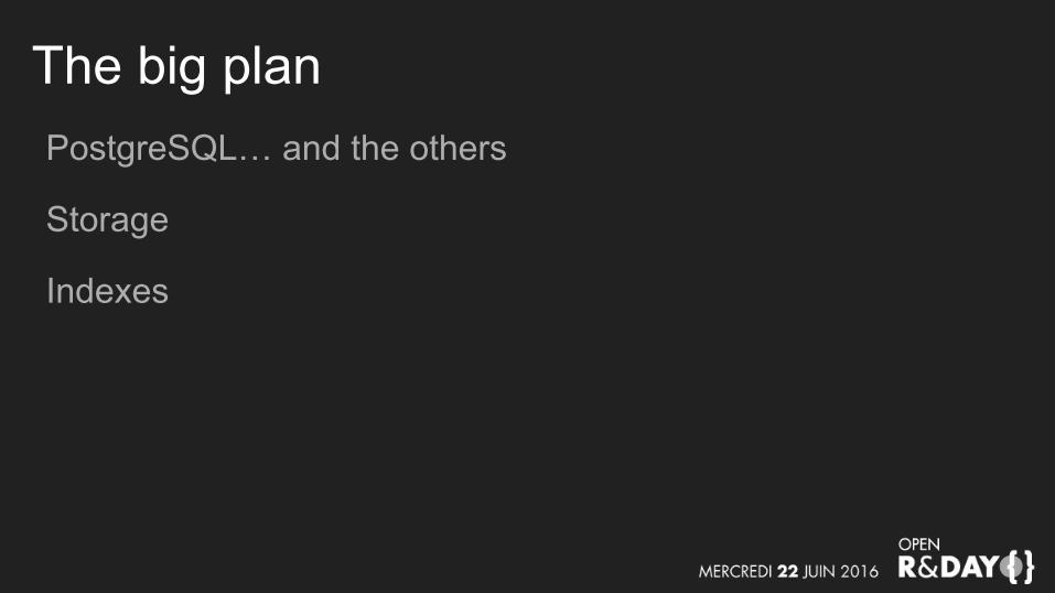
The big plan

The big planPostgreSQL… PostgreSQL… and the others

The big planPostgreSQL… and the others
Storage
The big planPostgreSQL… and the others
Storage
Indexes
The big planPostgreSQL… and the others
Storage
Indexes
Algorithms, algorithms everywhere!

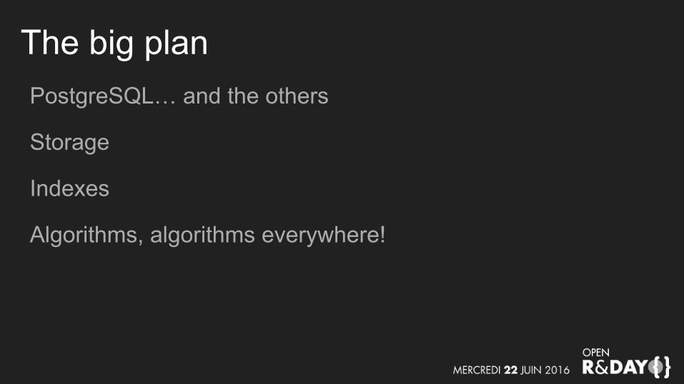
The big planPostgreSQL… and the others
Storage
Indexes
Algorithms, algorithms everywhere!

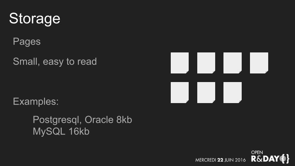
Pages
Small, easy to read
Storage
Pages
Small, easy to read
Examples:
Storage
Postgresql, Oracle 8kbMySQL 16kb
Simple table, values:
● id: integer● value: text
Storage
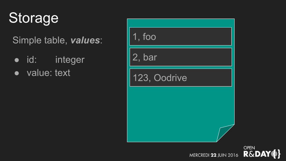
Simple table, values:
● id: integer● value: text
Storage1, foo
2, bar
123, Oodrive

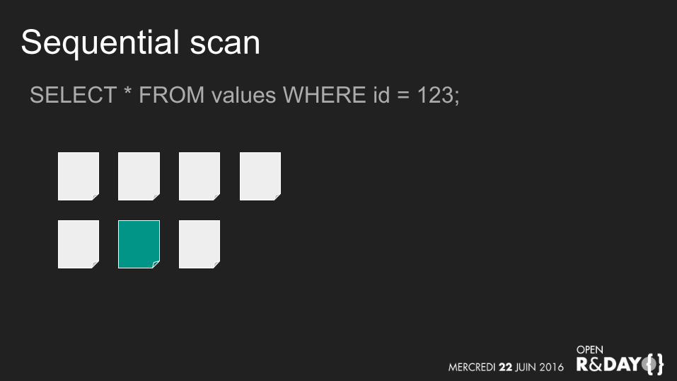
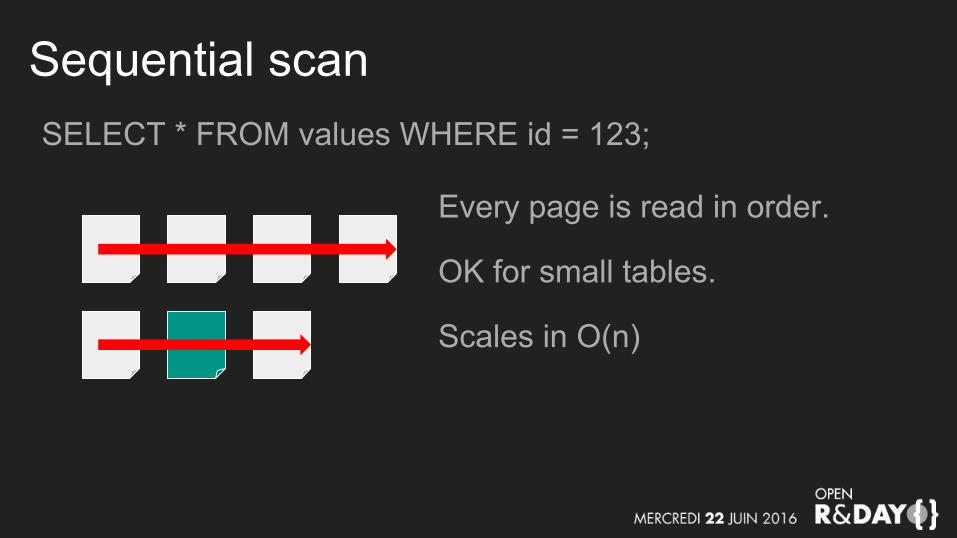
Sequential scanSELECT * FROM values WHERE id = 123;
Sequential scanSELECT * FROM values WHERE id = 123;
Sequential scanSELECT * FROM values WHERE id = 123;
Every page is read in order.
OK for small tables.
Scales in O(n)

Indexes
IndexesIn the beginning was the binary search tree
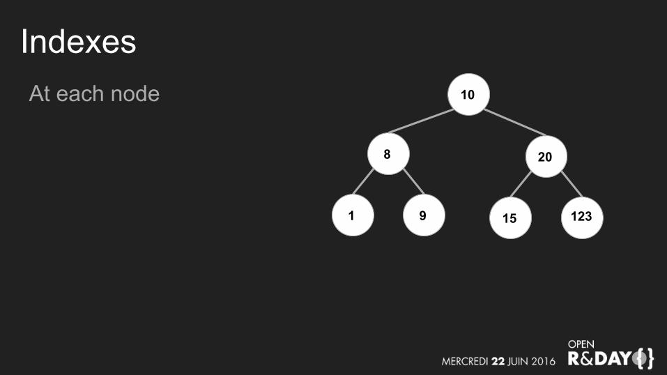
IndexesAt each node 10
8
1 9
20
15 123
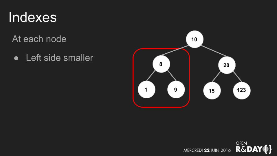
IndexesAt each node
● Left side smaller
10
8
1 9
20
15 123
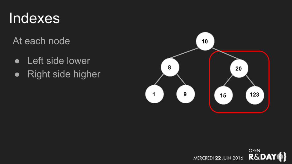
IndexesAt each node
● Left side lower● Right side higher
10
8
1 9
20
15 123
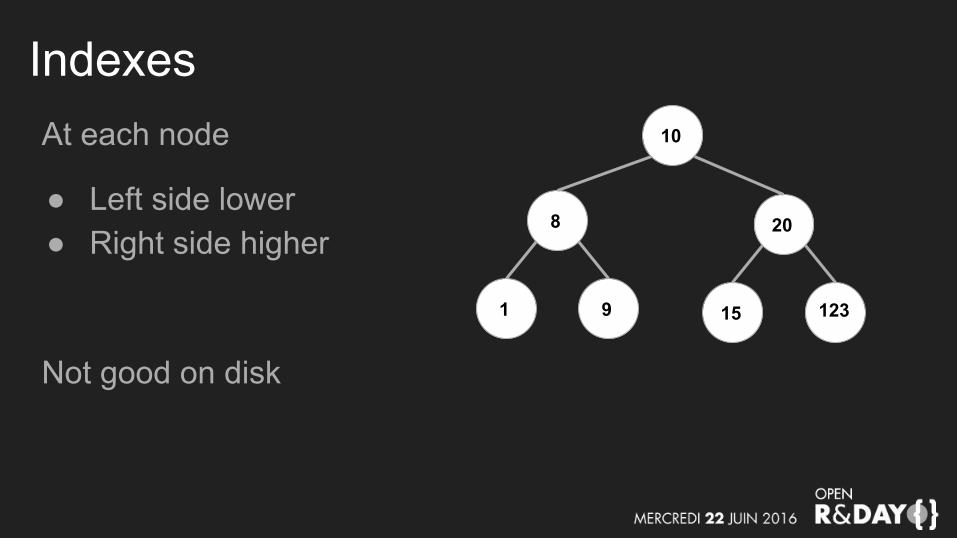
IndexesAt each node
● Left side lower● Right side higher
Not good on disk
10
8
1 9
20
15 123

IndexesLet’s complicate things

IndexesLet’s complicate things
Here comes the B-tree
IndexesLet’s complicate things
Here comes the B-tree
(Nobody knows what the B means…)
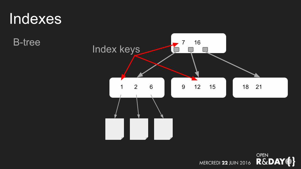
IndexesB-tree 7 16
9 12 151 2 6 2118
Index keys
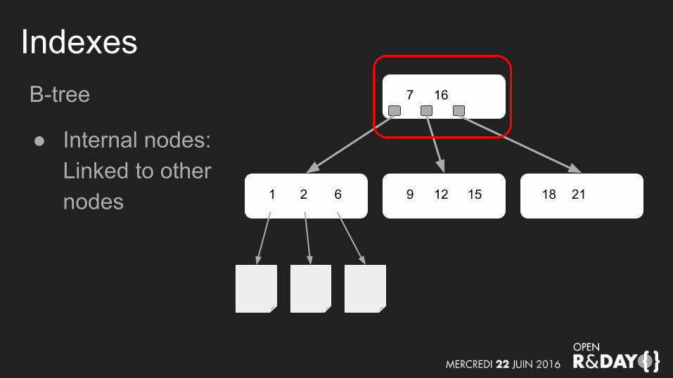
IndexesB-tree
● Internal nodes:Linked to other nodes
7 16
9 12 151 2 6 2118
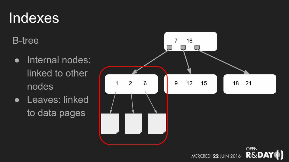
IndexesB-tree
● Internal nodes:linked to other nodes
● Leaves: linked to data pages
7 16
9 12 151 2 6 2118
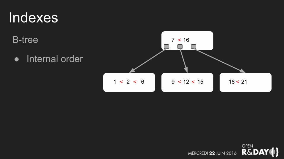
IndexesB-tree
● Internal order
7 16
9 12 151 2 6 2118
<
< < < < <
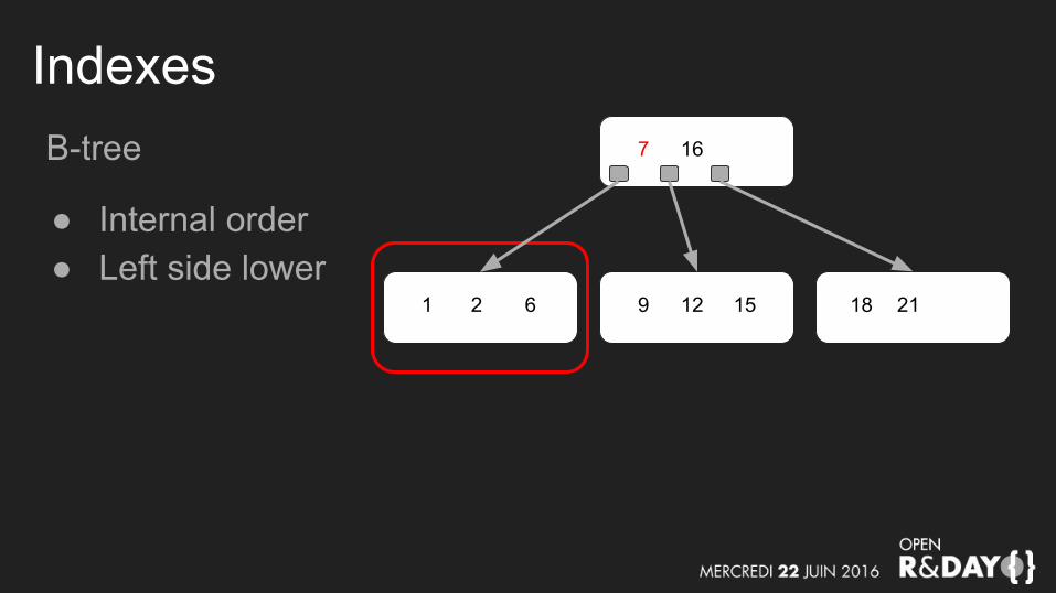
IndexesB-tree
● Internal order● Left side lower
7 16
9 12 151 2 6 2118

IndexesB-tree
● Internal order● Left side lower● Right side higher
7 16
9 12 151 2 6 2118
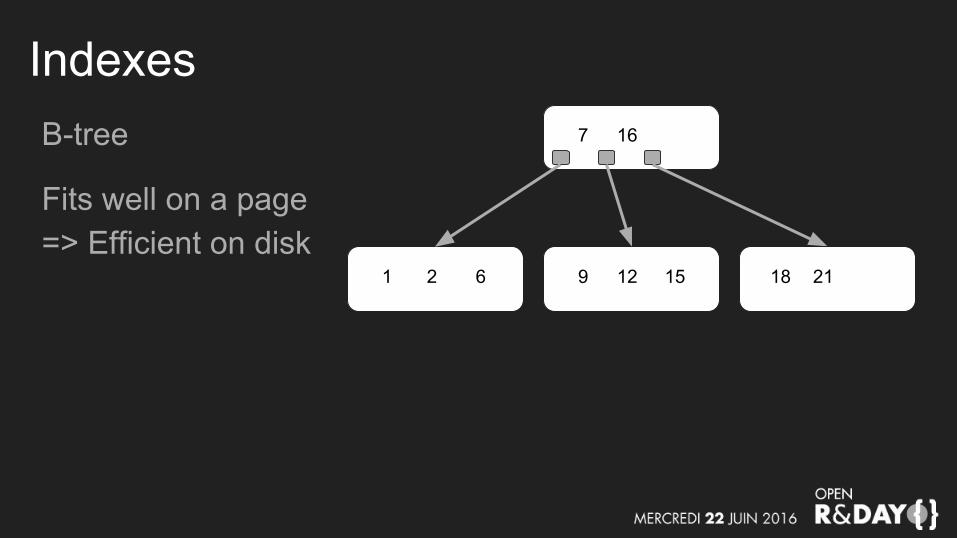
IndexesB-tree
Fits well on a page=> Efficient on disk
7 16
9 12 151 2 6 2118

What can we do with B-trees?Finding a single value
Let’s look for 12
7 16
9 12 151 2 6 2118
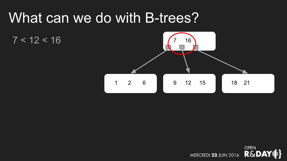
What can we do with B-trees?7 < 12 < 16 7 16
9 12 151 2 6 2118
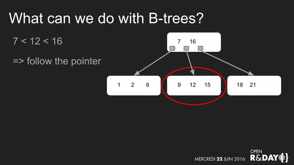
What can we do with B-trees?7 < 12 < 16
=> follow the pointer
7 16
9 12 151 2 6 2118

What can we do with B-trees?7 < 12 < 16
=> follow the pointer
Find it in the page
7 16
9 12 151 2 6 2118

What can we do with B-trees?7 < 12 < 16
=> follow the pointer
Find it in the page
Complexity O(log(n))
7 16
9 12 151 2 6 2118
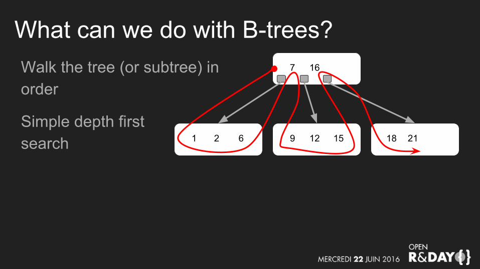
What can we do with B-trees?Walk the tree (or subtree) in order
Simple depth firstsearch
7 16
9 12 151 2 6 2118

What can we do with B-trees?Walk the tree (or subtree) in order
=> Answer ORDER BY queries
7 16
9 12 151 2 6 2118
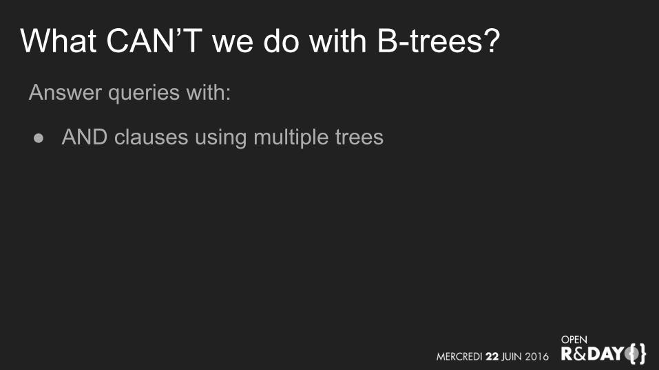
What CAN’T we do with B-trees?Answer queries with:
● AND clauses using multiple trees
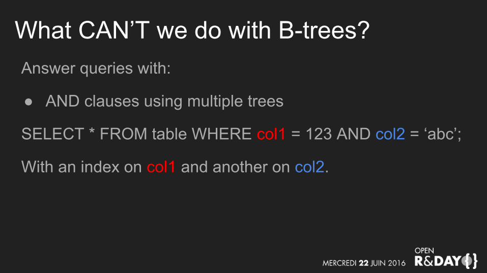
What CAN’T we do with B-trees?Answer queries with:
● AND clauses using multiple trees
SELECT * FROM table WHERE col1 = 123 AND col2 = ‘abc’;
With an index on col1 and another on col2.
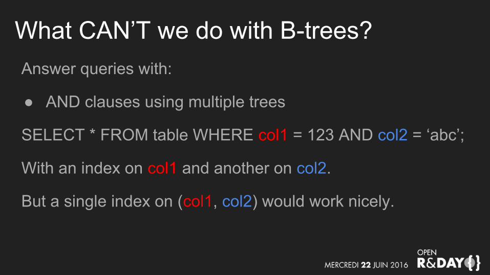
What CAN’T we do with B-trees?Answer queries with:
● AND clauses using multiple trees
SELECT * FROM table WHERE col1 = 123 AND col2 = ‘abc’;
With an index on col1 and another on col2.
But a single index on (col1, col2) would work nicely.
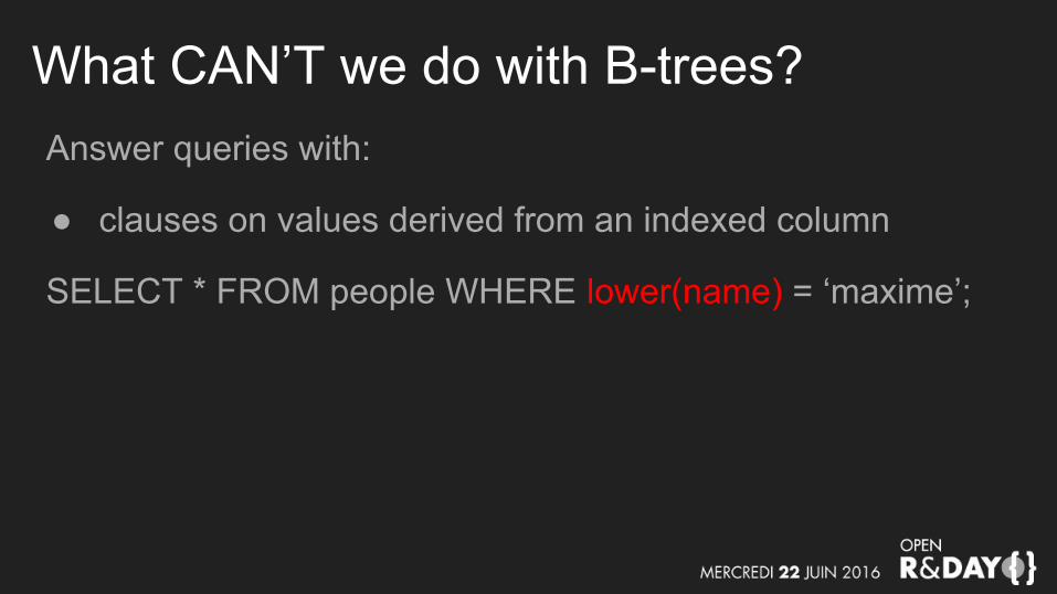
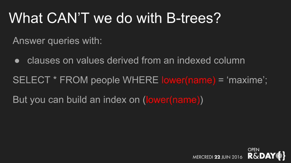
What CAN’T we do with B-trees?Answer queries with:
● clauses on values derived from an indexed column
SELECT * FROM people WHERE lower(name) = ‘maxime’;
What CAN’T we do with B-trees?Answer queries with:
● clauses on values derived from an indexed column
SELECT * FROM people WHERE lower(name) = ‘maxime’;
But you can build an index on (lower(name))
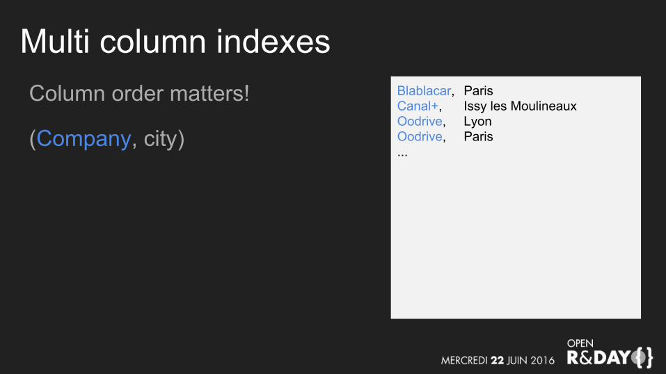
Multi column indexesColumn order matters!
(Company, city)
Blablacar, ParisCanal+, Issy les MoulineauxOodrive, LyonOodrive, Paris...
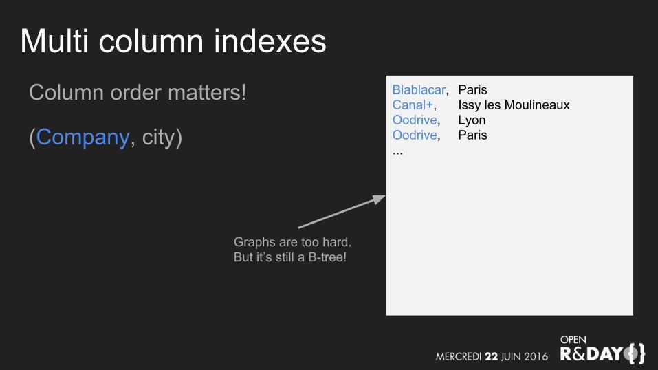
Multi column indexesColumn order matters!
(Company, city)
Blablacar, ParisCanal+, Issy les MoulineauxOodrive, LyonOodrive, Paris...
Graphs are too hard.But it’s still a B-tree!
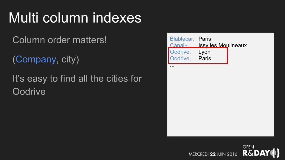
Multi column indexesColumn order matters!
(Company, city)
It’s easy to find all the cities for Oodrive
Blablacar, ParisCanal+, Issy les MoulineauxOodrive, LyonOodrive, Paris...
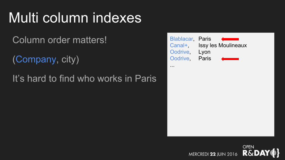
Multi column indexesColumn order matters!
(Company, city)
It’s hard to find who works in Paris
Blablacar, ParisCanal+, Issy les MoulineauxOodrive, LyonOodrive, Paris...
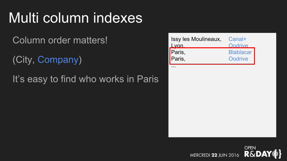
Multi column indexesColumn order matters!
(City, Company)
It’s easy to find who works in Paris
Issy les Moulineaux, Canal+Lyon, OodriveParis, BlablacarParis, Oodrive...
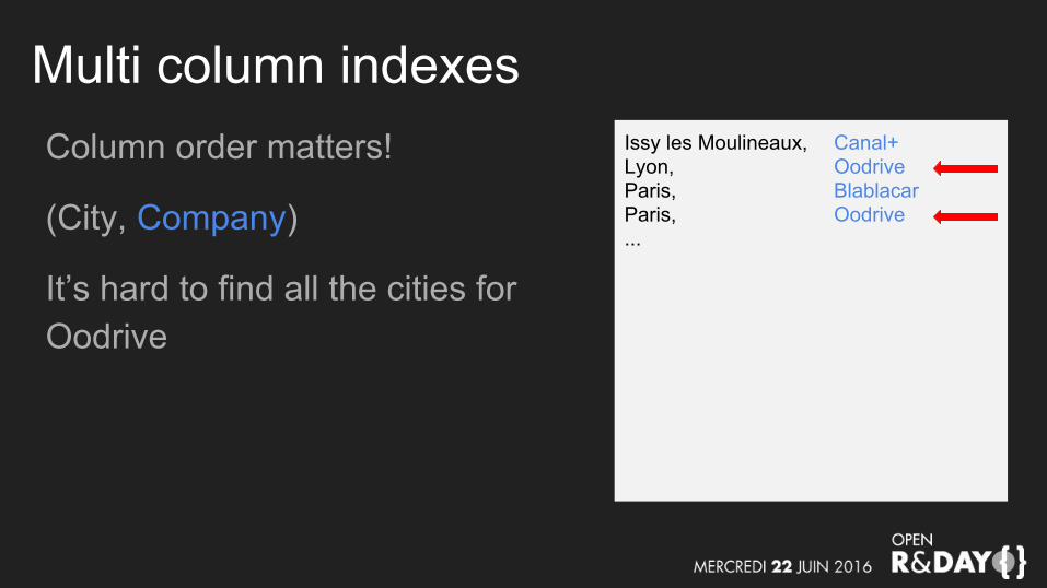
Multi column indexesColumn order matters!
(City, Company)
It’s hard to find all the cities for Oodrive
Issy les Moulineaux, Canal+Lyon, OodriveParis, BlablacarParis, Oodrive...
Joining tables

Joining tablesSELECT * FROM table1
JOIN table2 USING (joinColumn1)
WHERE ...;
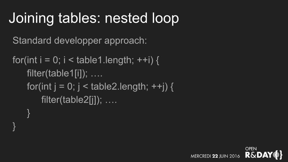
Joining tables: nested loopStandard developper approach:
for(int i = 0; i < table1.length; ++i) {filter(table1[i]); ….for(int j = 0; j < table2.length; ++j) {
filter(table2[j]); ….}
}
Joining tables: nested loopWorks well if:
● the first table is small,● the second table has an index on the join column.
Joining tables: nested loopWorks well if:
● the first table is small,● the second table has an index on the join column.
Doesn’t if:
● the join condition is complex
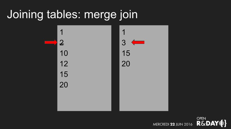
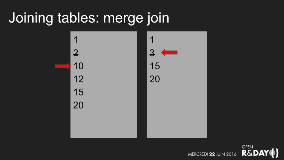
Joining tables: merge joinSort the two sides of the join on the index condition
Iterate both sides to find common values.
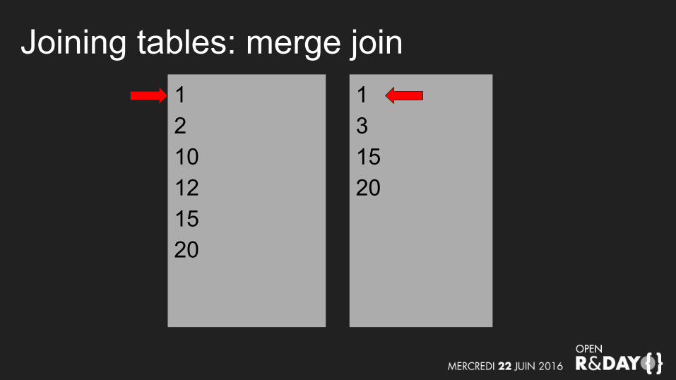
Joining tables: merge join1210121520
131520
Joining tables: merge join1210121520
131520
Joining tables: merge join1210121520
131520

Joining tables: merge joinWorks well if:
● both sides can be filtered and sorted cheaply● both sides are big
Best strategy for full outer joins
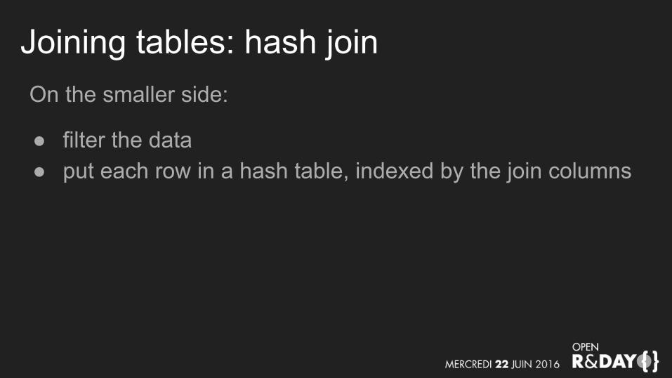
Joining tables: hash joinOn the smaller side:
● filter the data● put each row in a hash table, indexed by the join columns
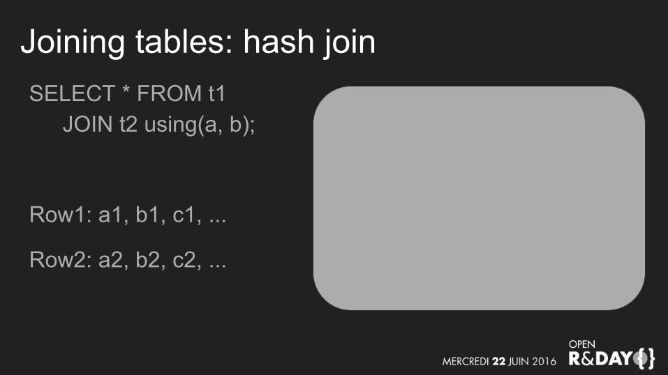
Joining tables: hash joinSELECT * FROM t1
JOIN t2 using(a, b);
Row1: a1, b1, c1, ...
Row2: a2, b2, c2, ...
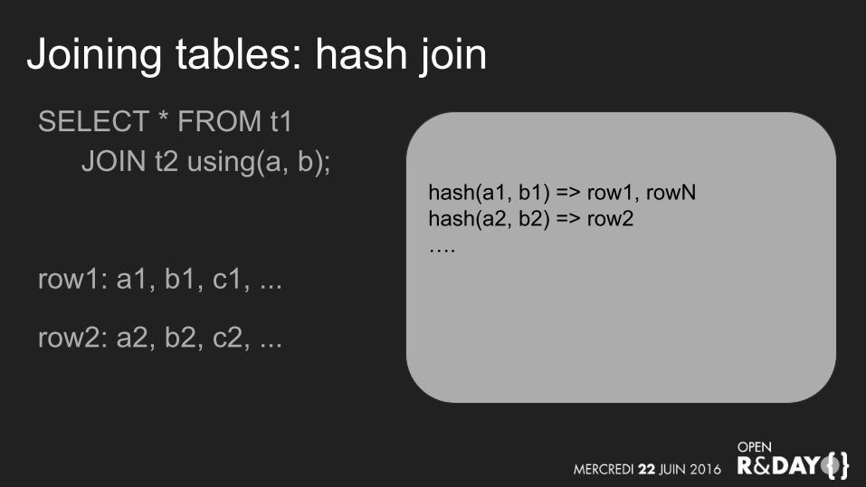
Joining tables: hash joinSELECT * FROM t1
JOIN t2 using(a, b);
row1: a1, b1, c1, ...
row2: a2, b2, c2, ...
hash(a1, b1) => row1, rowNhash(a2, b2) => row2….
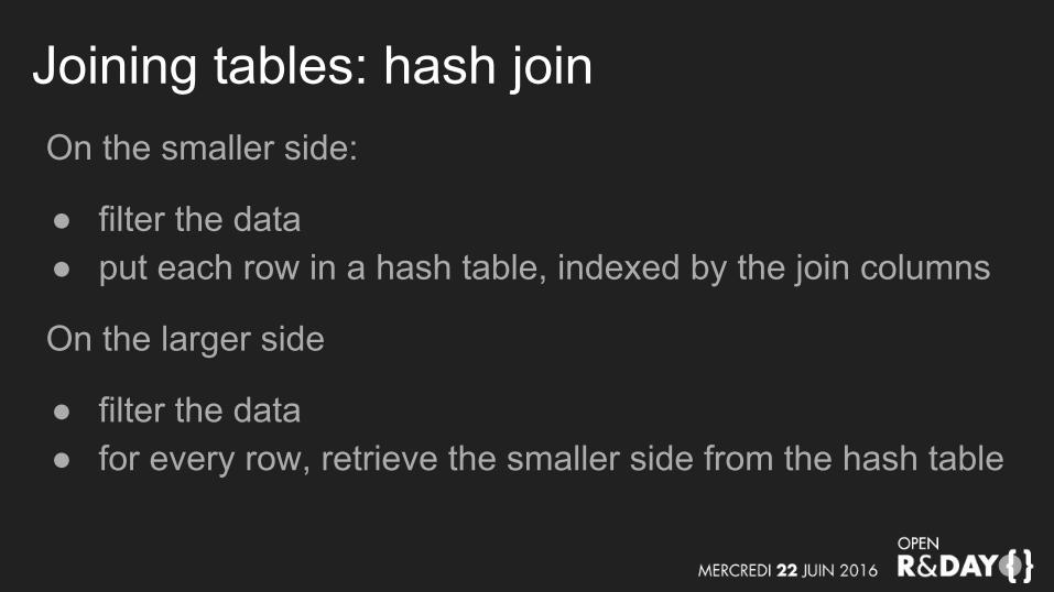
Joining tables: hash joinOn the smaller side:
● filter the data● put each row in a hash table, indexed by the join columns
On the larger side
● filter the data● for every row, retrieve the smaller side from the hash table

Joining tables: hash joinSELECT * FROM t1
JOIN t2 using(a, b);
row1: a1, b1, c1, ...
row2: a2, b2, c2, ...
hash(a1, b1) => row1, rowNhash(a2, b2) => row2….
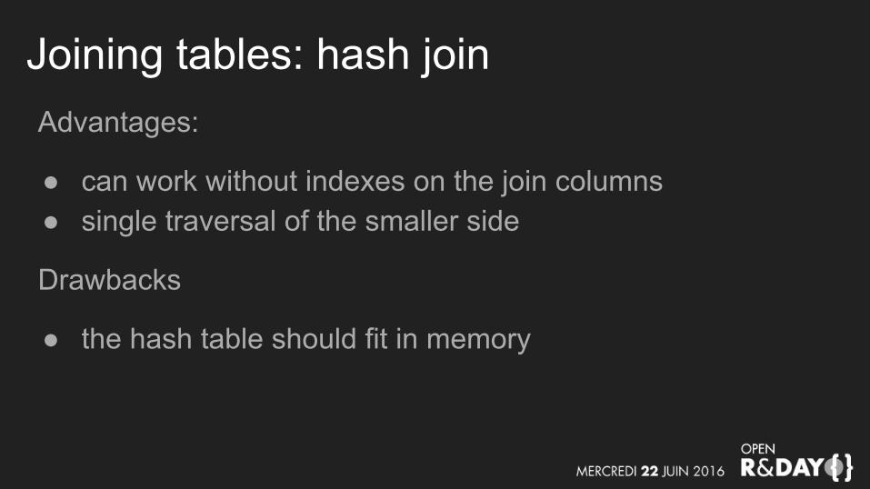
Joining tables: hash joinAdvantages:
● can work without indexes on the join columns● single traversal of the smaller side
Drawbacks
● the hash table should fit in memory
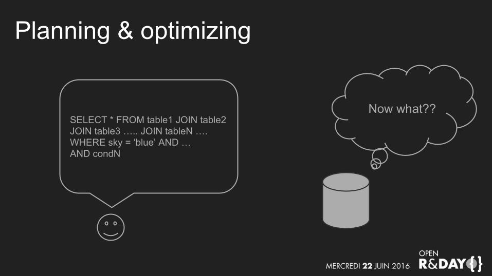
Planning & optimizing
Now what??SELECT * FROM table1 JOIN table2JOIN table3 ….. JOIN tableN ….WHERE sky = ‘blue’ AND …AND condN
Planning & optimizingGoal: least possible work
=> read as little as possible
Planning & optimizingThe tools:
● a query tree that can be modified● cardinality estimation for column values
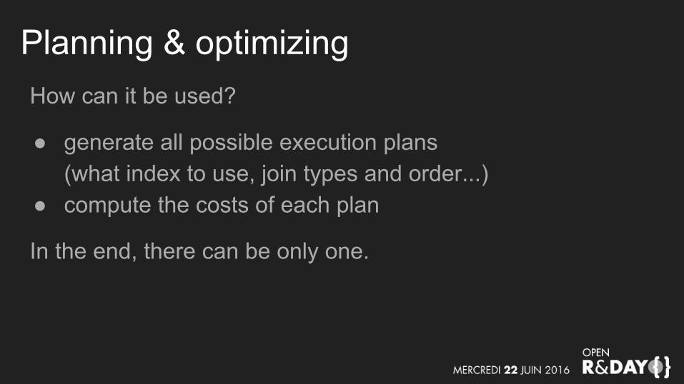
Planning & optimizingHow can it be used?
● generate all possible execution plans(what index to use, join types and order...)
● compute the costs of each plan
Planning & optimizingHow can it be used?
● generate all possible execution plans(what index to use, join types and order...)
● compute the costs of each plan
In the end, there can be only one.
Planning & optimizing
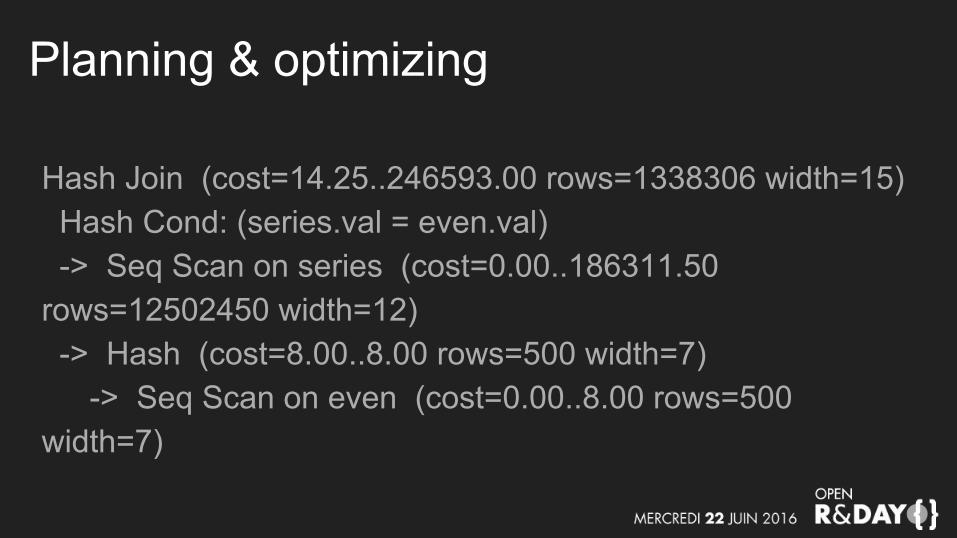
Hash Join (cost=14.25..246593.00 rows=1338306 width=15) Hash Cond: (series.val = even.val) -> Seq Scan on series (cost=0.00..186311.50 rows=12502450 width=12) -> Hash (cost=8.00..8.00 rows=500 width=7) -> Seq Scan on even (cost=0.00..8.00 rows=500 width=7)
Planning & optimizing
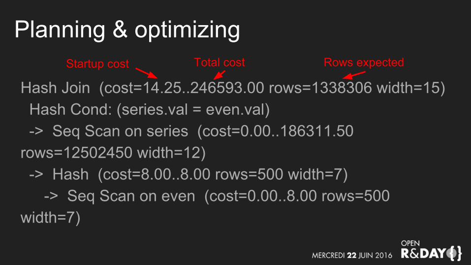
Hash Join (cost=14.25..246593.00 rows=1338306 width=15) Hash Cond: (series.val = even.val) -> Seq Scan on series (cost=0.00..186311.50 rows=12502450 width=12) -> Hash (cost=8.00..8.00 rows=500 width=7) -> Seq Scan on even (cost=0.00..8.00 rows=500 width=7)
Startup cost Total cost Rows expected

CaveatsLet’s index everything!
CaveatsLet’s index everything!
Index only what you need, they are costly
CaveatsLet’s index everything!
Index only what you need, indexes are costly
Small dataset, small gains
Other interesting things● data modification & MVCC
(Multiversion concurrency control)
How are transactions represented?How do we keep uncommitted writes from being read?
Other interesting things● data modification & MVCC
(Multiversion concurrency control)● replication
What are the tradeoffs between consistency and availability?
Other interesting things● data modification & MVCC
(Multiversion concurrency control)● replication● other index types
Inverted indexes, bitmap, hash, spatial...

The end

Oh, you had questions?