DBMS Storage - cs.iit.educs425/slides/ch11-indexing-and-storage-handout.pdf · Rotational latency...
13
1 Modified from: Database System Concepts, 6 th Ed. ©Silberschatz, Korth and Sudarshan See www.db-book.com for conditions on re-use Chapter 11: Indexing and Storage ©Silberschatz, Korth and Sudarshan 11.2 CS425 – Fall 2013 – Boris Glavic Chapter 11: Indexing and Storage ■ DBMS Storage ● Memory hierarchy ● File Organization ● Buffering ■ Indexing ● Basic Concepts ● B + -Trees ● Static Hashing ● Index Definition in SQL ● Multiple-Key Access Modified from: Database System Concepts, 6 th Ed. ©Silberschatz, Korth and Sudarshan See www.db-book.com for conditions on re-use Memory Hierarchy ©Silberschatz, Korth and Sudarshan 11.4 CS425 – Fall 2013 – Boris Glavic DBMS Storage ■ Modern Computers have different types of memory ● Cache, Main Memory, Harddisk, SSD, … ■ Memory types have different characteristics in terms of ● Persistent vs. volatile ● Speed (random vs. sequential access) ● Size ● Price – this usually determines size ■ Database systems are designed to be use these different memory types effectively ● Need for persistent storage: the state of the database needs to be written to persistent storage ! guarantee database content is not lost when the computer is shutdown ● Moving data between different types of memory ! Want to use fast memory to speed-up operations ! Need slower memory for the size ©Silberschatz, Korth and Sudarshan 11.5 CS425 – Fall 2013 – Boris Glavic Storage Hierarchy cache main memory flash memory magnetic disk optical disk magnetic tapes Size Speed Persistent storage ©Silberschatz, Korth and Sudarshan 11.6 CS425 – Fall 2013 – Boris Glavic Main Memory vs. Disk ■ Why do we not only use main memory ● What if database does not fit into main memory? ● Main memory is volatile ■ Main memory vs. disk ● Given available main memory when do we keep which part of the database in main memory ! Buffer manager: Component of DBMS that decides when to move data between disk and main memory ● How do we ensure transaction property durability ! Buffer manager needs to make sure data written by committed transactions is written to disk to ensure durability
Transcript of DBMS Storage - cs.iit.educs425/slides/ch11-indexing-and-storage-handout.pdf · Rotational latency...
1!
Modified from:!Database System Concepts, 6th Ed.!
©Silberschatz, Korth and SudarshanSee www.db-book.com for conditions on re-use !
Chapter 11: Indexing and Storage!
©Silberschatz, Korth and Sudarshan!11.2!CS425 – Fall 2013 – Boris Glavic!
Chapter 11: Indexing and Storage!
■ DBMS Storage!● Memory hierarchy!● File Organization!● Buffering!
■ Indexing!● Basic Concepts!● B+-Trees!● Static Hashing!● Index Definition in SQL!● Multiple-Key Access!
Modified from:!Database System Concepts, 6th Ed.!
©Silberschatz, Korth and SudarshanSee www.db-book.com for conditions on re-use !
Memory Hierarchy!
©Silberschatz, Korth and Sudarshan!11.4!CS425 – Fall 2013 – Boris Glavic!
DBMS Storage!
■ Modern Computers have different types of memory!● Cache, Main Memory, Harddisk, SSD, …!
■ Memory types have different characteristics in terms of!● Persistent vs. volatile!● Speed (random vs. sequential access)!● Size!● Price – this usually determines size!
■ Database systems are designed to be use these different memory types effectively!● Need for persistent storage: the state of the database needs to be
written to persistent storage !! guarantee database content is not lost when the computer is
shutdown!● Moving data between different types of memory!
! Want to use fast memory to speed-up operations!! Need slower memory for the size!
©Silberschatz, Korth and Sudarshan!11.5!CS425 – Fall 2013 – Boris Glavic!
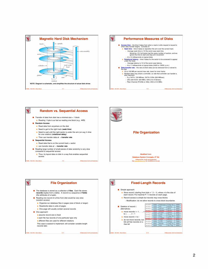
Storage Hierarchy!cache
main memory
flash memory
magnetic disk
optical disk
magnetic tapes
Size!
Spee
d!
Persistent!storage!
©Silberschatz, Korth and Sudarshan!11.6!CS425 – Fall 2013 – Boris Glavic!
Main Memory vs. Disk!
■ Why do we not only use main memory!● What if database does not fit into main memory?!● Main memory is volatile!
■ Main memory vs. disk!● Given available main memory when do we keep which part of the
database in main memory!! Buffer manager: Component of DBMS that decides when to
move data between disk and main memory!● How do we ensure transaction property durability!
! Buffer manager needs to make sure data written by committed transactions is written to disk to ensure durability!
2!
©Silberschatz, Korth and Sudarshan!11.7!CS425 – Fall 2013 – Boris Glavic!
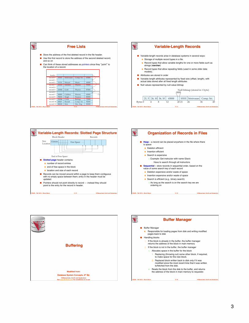
Magnetic Hard Disk Mechanism!
NOTE: Diagram is schematic, and simplifies the structure of actual disk drives!
track t
sector s
spindle
cylinder c
platterarm
read–writehead
arm assembly
rotation
©Silberschatz, Korth and Sudarshan!11.8!CS425 – Fall 2013 – Boris Glavic!
Performance Measures of Disks!■ Access time – the time it takes from when a read or write request is issued to
when data transfer begins. Consists of: !● Seek time – time it takes to reposition the arm over the correct track. !
! Average seek time is 1/2 the worst case seek time.!– Would be 1/3 if all tracks had the same number of sectors, and we
ignore the time to start and stop arm movement!! 4 to 10 milliseconds on typical disks!
● Rotational latency – time it takes for the sector to be accessed to appear under the head. !! Average latency is 1/2 of the worst case latency.!! 4 to 11 milliseconds on typical disks (5400 to 15000 r.p.m.)!
■ Data-transfer rate – the rate at which data can be retrieved from or stored to the disk.!● 25 to 100 MB per second max rate, lower for inner tracks!● Multiple disks may share a controller, so rate that controller can handle is
also important!! E.g. SATA: 150 MB/sec, SATA-II 3Gb (300 MB/sec)!! Ultra 320 SCSI: 320 MB/s, SAS (3 to 6 Gb/sec)!! Fiber Channel (FC2Gb or 4Gb): 256 to 512 MB/s!
©Silberschatz, Korth and Sudarshan!11.9!CS425 – Fall 2013 – Boris Glavic!
Random vs. Sequential Access!
■ Transfer of data from disk has a minimal size = 1 block!● Reading 1 byte is as fast as reading one block (e.g., 4KB)!
■ Random Access!● Read data from anywhere on the disk!● Need to get to the right track (seek time)!● Need to wait until the right sector is under the arm (on avg ½ time
for one rotation) (rotational delay)!● Then can transfer data at ~ transfer rate!
■ Sequential Access!● Read data that is on the current track + sector!● can transfer data at ~ transfer rate!
■ Reading large number of small pieces of data randomly is very slow compared to sequential access!● Thus, try layout data on disk in a way that enables sequential
access!Modified from:!
Database System Concepts, 6th Ed.!©Silberschatz, Korth and Sudarshan
See www.db-book.com for conditions on re-use !
File Organization!
©Silberschatz, Korth and Sudarshan!11.11!CS425 – Fall 2013 – Boris Glavic!
File Organization!
■ The database is stored as a collection of files. Each file stores records (tuples from a table). A record is a sequence of fields (the attributes of a tuple).!
■ Reading one record of a time from disk would be very slow (random access)!● Organize our database files in pages (size of block or larger)!● Read/write data in units of pages!● One page will usually contain several records!
■ One approach:!● assume record size is fixed!● each file has records of one particular type only !● different files are used for different relations!This case is easiest to implement; will consider variable length records later.!
©Silberschatz, Korth and Sudarshan!11.12!CS425 – Fall 2013 – Boris Glavic!
Fixed-Length Records!
■ Simple approach:!● Store record i starting from byte n * (i – 1), where n is the size of
each record. Put maximal P / n records on each page.!● Record access is simple but records may cross blocks!
! Modification: do not allow records to cross block boundaries!!
■ Deletion of record i: alternatives:"● move records i + 1, . . ., n
to i, . . . , n – 1!● move record n to i!● do not move records, but
link all free records on a free list!
Srinivasan Comp. Sci. 65000Wu Finance 90000Mozart Music 40000Einstein Physics 95000El Said History 60000Gold Physics 87000Katz Comp. Sci. 75000Califieri History 62000Singh Finance 80000Crick Biology 72000Brandt Comp. Sci. 92000
15151
1010112121
222223234333456455655858376543767668382198345 Kim Elec. Eng. 80000
record 0record 1record 2record 3record 4record 5record 6record 7record 8record 9record 10record 11
3!
©Silberschatz, Korth and Sudarshan!11.13!CS425 – Fall 2013 – Boris Glavic!
Free Lists!
■ Store the address of the first deleted record in the file header.!■ Use this first record to store the address of the second deleted record,
and so on!■ Can think of these stored addresses as pointers since they “point” to
the location of a record.!
headerrecord 0record 1record 2record 3record 4record 5record 6record 7record 8record 9record 10record 11
720009200080000
65000
4000095000
87000
62000
767668382198345
10101
1515122222
33456
5858376543
CrickBrandtKim
Srinivasan
MozartEinstein
Gold
CalifieriSingh
Biology
Elec. Eng.
Comp. Sci.
Comp. Sci.
MusicPhysics
Physics
HistoryFinance 80000
©Silberschatz, Korth and Sudarshan!11.14!CS425 – Fall 2013 – Boris Glavic!
Variable-Length Records!
■ Variable-length records arise in database systems in several ways:!● Storage of multiple record types in a file.!● Record types that allow variable lengths for one or more fields such as
strings (varchar)!● Record types that allow repeating fields (used in some older data
models).!■ Attributes are stored in order!■ Variable length attributes represented by fixed size (offset, length), with
actual data stored after all fixed length attributes!■ Null values represented by null-value bitmap!!
21, 5 26, 10 36, 10 65000 10101 Srinivasan Comp. Sci.Bytes 0 4 8 12 20 21 26 36 45
0000Null bitmap (stored in 1 byte)
©Silberschatz, Korth and Sudarshan!11.15!CS425 – Fall 2013 – Boris Glavic!
Variable-Length Records: Slotted Page Structure!
■ Slotted page header contains:!● number of record entries!● end of free space in the block!● location and size of each record!
■ Records can be moved around within a page to keep them contiguous with no empty space between them; entry in the header must be updated.!
■ Pointers should not point directly to record — instead they should point to the entry for the record in header.!
# EntriesSizeLocation
Block Header Records
Free Space
End of Free Space
©Silberschatz, Korth and Sudarshan!11.16!CS425 – Fall 2013 – Boris Glavic!
Organization of Records in Files!
■ Heap – a record can be placed anywhere in the file where there is space!● Deletion efficient!● Insertion efficient!● Search is expensive!
! Example: Get instructor with name Glavic!– Have to search through all instructors!
■ Sequential – store records in sequential order, based on the value of some search key of each record!● Deletion expensive and/or waste of space!● Insertion expensive and/or waste of space!● Search is efficient (e.g., binary search)!
! As long as the search is on the search key we are ordering on!
Modified from:!Database System Concepts, 6th Ed.!
©Silberschatz, Korth and SudarshanSee www.db-book.com for conditions on re-use !
Buffering!
©Silberschatz, Korth and Sudarshan!11.18!CS425 – Fall 2013 – Boris Glavic!
Buffer Manager!
■ Buffer Manager!● Responsible for loading pages from disk and writing modified
pages back to disk!■ Handling blocks!
1. If the block is already in the buffer, the buffer manager returns the address of the block in main memory!
2. If the block is not in the buffer, the buffer manager!1. Allocates space in the buffer for the block!
1. Replacing (throwing out) some other block, if required, to make space for the new block.!
2. Replaced block written back to disk only if it was modified since the most recent time that it was written to/fetched from the disk.!
2. Reads the block from the disk to the buffer, and returns the address of the block in main memory to requester. !
4!
©Silberschatz, Korth and Sudarshan!11.19!CS425 – Fall 2013 – Boris Glavic!
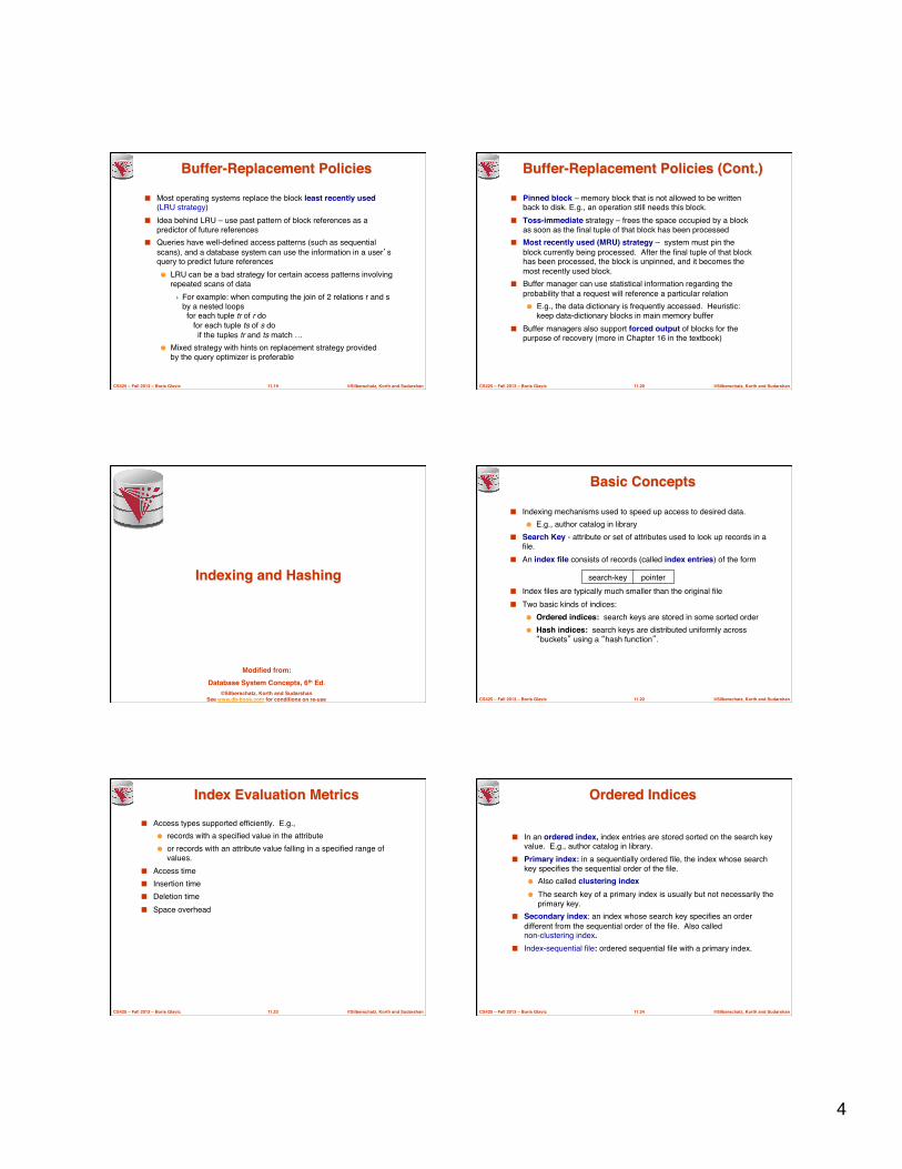
Buffer-Replacement Policies!
■ Most operating systems replace the block least recently used (LRU strategy)!
■ Idea behind LRU – use past pattern of block references as a predictor of future references!
■ Queries have well-defined access patterns (such as sequential scans), and a database system can use the information in a user’s query to predict future references!● LRU can be a bad strategy for certain access patterns involving
repeated scans of data!! For example: when computing the join of 2 relations r and s
by a nested loops for each tuple tr of r do for each tuple ts of s do if the tuples tr and ts match …!
● Mixed strategy with hints on replacement strategy provided by the query optimizer is preferable!
©Silberschatz, Korth and Sudarshan!11.20!CS425 – Fall 2013 – Boris Glavic!
Buffer-Replacement Policies (Cont.)!
■ Pinned block – memory block that is not allowed to be written back to disk. E.g., an operation still needs this block.!
■ Toss-immediate strategy – frees the space occupied by a block as soon as the final tuple of that block has been processed!
■ Most recently used (MRU) strategy – system must pin the block currently being processed. After the final tuple of that block has been processed, the block is unpinned, and it becomes the most recently used block.!
■ Buffer manager can use statistical information regarding the probability that a request will reference a particular relation!● E.g., the data dictionary is frequently accessed. Heuristic:
keep data-dictionary blocks in main memory buffer!■ Buffer managers also support forced output of blocks for the
purpose of recovery (more in Chapter 16 in the textbook)!
Modified from:!Database System Concepts, 6th Ed.!
©Silberschatz, Korth and SudarshanSee www.db-book.com for conditions on re-use !
Indexing and Hashing!
©Silberschatz, Korth and Sudarshan!11.22!CS425 – Fall 2013 – Boris Glavic!
Basic Concepts!
■ Indexing mechanisms used to speed up access to desired data.!● E.g., author catalog in library!
■ Search Key - attribute or set of attributes used to look up records in a file.!
■ An index file consists of records (called index entries) of the form!
■ Index files are typically much smaller than the original file !■ Two basic kinds of indices:!
● Ordered indices: search keys are stored in some sorted order!● Hash indices: search keys are distributed uniformly across “buckets” using a “hash function”. !
search-key! pointer!
©Silberschatz, Korth and Sudarshan!11.23!CS425 – Fall 2013 – Boris Glavic!
Index Evaluation Metrics!
■ Access types supported efficiently. E.g., !● records with a specified value in the attribute!● or records with an attribute value falling in a specified range of
values.!■ Access time!■ Insertion time!■ Deletion time!■ Space overhead!
©Silberschatz, Korth and Sudarshan!11.24!CS425 – Fall 2013 – Boris Glavic!
Ordered Indices!
■ In an ordered index, index entries are stored sorted on the search key value. E.g., author catalog in library.!
■ Primary index: in a sequentially ordered file, the index whose search key specifies the sequential order of the file.!● Also called clustering index!● The search key of a primary index is usually but not necessarily the
primary key.!■ Secondary index: an index whose search key specifies an order
different from the sequential order of the file. Also called non-clustering index.!
■ Index-sequential file: ordered sequential file with a primary index.!

5!
©Silberschatz, Korth and Sudarshan!11.25!CS425 – Fall 2013 – Boris Glavic!
Secondary Indices Example!
■ Index record points to a bucket that contains pointers to all the actual records with that particular search-key value.!
■ Secondary indices have to be dense!
Secondary index on salary field of instructor!
4000060000620006500072000750008000087000900009200095000
10101 Srinivasan Comp. Sci. 6500012121 Wu Finance 9000015151 Mozart Music 4000022222 Einstein Physics 9500032343 El Said History 6000033456 Gold Physics 8700045565 Katz Comp. Sci. 7500058583 Califieri History 6200076543 Singh Finance 8000076766 Crick Biology 7200083821 Brandt Comp. Sci. 9200098345 Kim Elec. Eng. 80000
©Silberschatz, Korth and Sudarshan!11.26!CS425 – Fall 2013 – Boris Glavic!
Primary and Secondary Indices!
■ Indices offer substantial benefits when searching for records.!■ BUT: Updating indices imposes overhead on database
modification --when a file is modified, every index on the file must be updated, !
■ Sequential scan using primary index is efficient, but a sequential scan using a secondary index is expensive !● Each record access may fetch a new block from disk!● Block fetch requires about 5 to 10 milliseconds, versus
about 100 nanoseconds for memory access!
©Silberschatz, Korth and Sudarshan!11.27!CS425 – Fall 2013 – Boris Glavic!
Multilevel Index!■ If primary index does not fit in memory, access becomes
expensive.!■ Solution: treat primary index kept on disk as a sequential file
and construct a sparse index on it.!● outer index – a sparse index of primary index!● inner index – the primary index file!
■ If even outer index is too large to fit in main memory, yet another level of index can be created, and so on.!
■ Indices at all levels must be updated on insertion or deletion from the file.!
©Silberschatz, Korth and Sudarshan!11.28!CS425 – Fall 2013 – Boris Glavic!
Multilevel Index (Cont.)!
…
……
…
outer index
indexblock 0
indexblock 1
datablock 0
datablock 1
inner index
©Silberschatz, Korth and Sudarshan!11.29!CS425 – Fall 2013 – Boris Glavic!
Index Update: Deletion!
■ Single-level index entry deletion:!● Dense indices – deletion of search-key is similar to file record
deletion.!● Sparse indices –!
! if an entry for the search key exists in the index, it is deleted by replacing the entry in the index with the next search-key value in the file (in search-key order). !
! If the next search-key value already has an index entry, the entry is deleted instead of being replaced.!
101013234376766
10101 Srinivasan
45565 Katz58583 Califieri76543 Singh76766 Crick83821 Brandt98345 Kim
12121 Wu15151 Mozart22222 Einstein32343 El Said33456 Gold
Comp. Sci.
Comp. Sci.
Comp. Sci.HistoryFinanceBiology
Elec. Eng.
FinanceMusicPhysicsHistoryPhysics
65000
750006200080000720009200080000
9000040000950006000087000■ If deleted record was the
only record in the file with its particular search-key value, the search-key is deleted from the index also.!
©Silberschatz, Korth and Sudarshan!11.30!CS425 – Fall 2013 – Boris Glavic!
Index Update: Insertion!
■ Single-level index insertion:!● Perform a lookup using the search-key value appearing in
the record to be inserted.!● Dense indices – if the search-key value does not appear in
the index, insert it.!● Sparse indices – if index stores an entry for each block of
the file, no change needs to be made to the index unless a new block is created. !! If a new block is created, the first search-key value
appearing in the new block is inserted into the index.!■ Multilevel insertion and deletion: algorithms are simple
extensions of the single-level algorithms!

6!
©Silberschatz, Korth and Sudarshan!11.31!CS425 – Fall 2013 – Boris Glavic!
Secondary Indices!
■ Frequently, one wants to find all the records whose values in a certain field (which is not the search-key of the primary index) satisfy some condition.!● Example 1: In the instructor relation stored sequentially by
ID, we may want to find all instructors in a particular department!
● Example 2: as above, but where we want to find all instructors with a specified salary or with salary in a specified range of values!
■ We can have a secondary index with an index record for each search-key value!
©Silberschatz, Korth and Sudarshan!11.32!CS425 – Fall 2013 – Boris Glavic!
B+-Tree Index!
■ Disadvantage of indexed-sequential files!● performance degrades as file grows, since many overflow
blocks get created. !● Periodic reorganization of entire file is required.!
■ Advantage of B+-tree index files: !● automatically reorganizes itself with small, local, changes,
in the face of insertions and deletions. !● Reorganization of entire file is not required to maintain
performance.!■ (Minor) disadvantage of B+-trees: !
● extra insertion and deletion overhead, space overhead.!■ Advantages of B+-trees outweigh disadvantages!
● B+-trees are used extensively!
B+-tree indices are an alternative to indexed-sequential files.!
©Silberschatz, Korth and Sudarshan!11.33!CS425 – Fall 2013 – Boris Glavic!
Example of B+-Tree!
Gold Katz Kim Mozart Singh Srinivasan Wu
Internal nodes
Root node
Leaf nodes
Einstein
Einstein El Said
Gold
Mozart
Srinivasan
Srinivasan Comp. Sci. 65000Wu Finance 90000Mozart Music 40000Einstein Physics 95000El Said History 80000Gold Physics 87000Katz Comp. Sci. 75000Califieri History 60000Singh Finance 80000Crick Biology 72000Brandt Comp. Sci. 92000
15151
10101
Brandt Califieri Crick
12121
222223234333456455655858376543767668382198345 Kim Elec. Eng. 80000
©Silberschatz, Korth and Sudarshan!11.34!CS425 – Fall 2013 – Boris Glavic!
B+-Tree Index Files (Cont.)!
■ All paths from root to leaf are of the same length!■ Each node that is not a root or a leaf has between ⎡n/2⎤ and
n children.!■ A leaf node has between ⎡(n–1)/2⎤ and n–1 values!■ Special cases: !
● If the root is not a leaf, it has at least 2 children.!● If the root is a leaf (that is, there are no other nodes in
the tree), it can have between 0 and (n–1) values.!
A B+-tree is a rooted tree satisfying the following properties:!
©Silberschatz, Korth and Sudarshan!11.35!CS425 – Fall 2013 – Boris Glavic!
B+-Tree Node Structure!
■ Typical node !● Ki are the search-key values !● Pi are pointers to children (for non-leaf nodes) or pointers to
records or buckets of records (for leaf nodes).!■ The search-keys in a node are ordered !! ! K1 < K2 < K3 < . . . < Kn–1!
(Initially assume no duplicate keys, address duplicates later)!!!!
P1 K1 P2 Pn-1 Kn-1 Pn…
©Silberschatz, Korth and Sudarshan!11.36!CS425 – Fall 2013 – Boris Glavic!
Leaf Nodes in B+-Trees!
■ For i = 1, 2, . . ., n–1, pointer Pi points to a file record with search-key value Ki, !
■ If Li, Lj are leaf nodes and i < j, Li’s search-key values are less than or equal to Lj’s search-key values!
■ Pn points to next leaf node in search-key order!
Properties of a leaf node:!
Srinivasan Comp. Sci. 65000Wu Finance 90000Mozart Music 40000Einstein Physics 95000El Said History 80000Gold Physics 87000Katz Comp. Sci. 75000Califieri History 60000Singh Finance 80000Crick Biology 72000Brandt Comp. Sci. 92000
15151
1010112121
222223234333456455655858376543767668382198345 Kim Elec. Eng. 80000
leaf nodePointer to next leaf nodeBrandt Califieri Crick
7!
©Silberschatz, Korth and Sudarshan!11.37!CS425 – Fall 2013 – Boris Glavic!
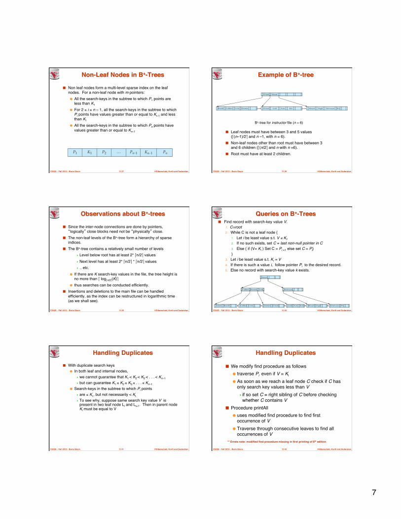
Non-Leaf Nodes in B+-Trees!
■ Non leaf nodes form a multi-level sparse index on the leaf nodes. For a non-leaf node with m pointers:!● All the search-keys in the subtree to which P1 points are
less than K1 !● For 2 ≤ i ≤ n – 1, all the search-keys in the subtree to which
Pi points have values greater than or equal to Ki–1 and less than Ki "
● All the search-keys in the subtree to which Pn points have values greater than or equal to Kn–1!
P1 K1 P2 Pn-1 Kn-1 Pn…
©Silberschatz, Korth and Sudarshan!11.38!CS425 – Fall 2013 – Boris Glavic!
Example of B+-tree!
■ Leaf nodes must have between 3 and 5 values (⎡(n–1)/2⎤ and n –1, with n = 6).!
■ Non-leaf nodes other than root must have between 3 and 6 children (⎡(n/2⎤ and n with n =6).!
■ Root must have at least 2 children.!
B+-tree for instructor file (n = 6)!
Brandt CrickCalifieri Einstein El Said Gold Katz Kim Mozart Singh Srinivasan Wu
El Said Mozart
©Silberschatz, Korth and Sudarshan!11.39!CS425 – Fall 2013 – Boris Glavic!
Observations about B+-trees!
■ Since the inter-node connections are done by pointers, “logically” close blocks need not be “physically” close.!
■ The non-leaf levels of the B+-tree form a hierarchy of sparse indices.!
■ The B+-tree contains a relatively small number of levels!! Level below root has at least 2* ⎡n/2⎤ values!! Next level has at least 2* ⎡n/2⎤ * ⎡n/2⎤ values!! .. etc.!
● If there are K search-key values in the file, the tree height is no more than ⎡ log⎡n/2⎤(K)⎤!
● thus searches can be conducted efficiently.!■ Insertions and deletions to the main file can be handled
efficiently, as the index can be restructured in logarithmic time (as we shall see).!
©Silberschatz, Korth and Sudarshan!11.40!CS425 – Fall 2013 – Boris Glavic!
Queries on B+-Trees!■ Find record with search-key value V."
1. C=root"2. While C is not a leaf node {!
1. Let i be least value s.t. V ≤ Ki.!2. If no such exists, set C = last non-null pointer in C !3. Else { if (V= Ki ) Set C = Pi +1 else set C = Pi}!}!
3. Let i be least value s.t. Ki = V"4. If there is such a value i, follow pointer Pi to the desired record.!5. Else no record with search-key value k exists.!
Adams Brandt Einstein El Said Gold Katz Kim Mozart Singh Srinivasan Wu
Gold Srinivasan
Mozart
EinsteinCalifieri
CrickCalifieri
©Silberschatz, Korth and Sudarshan!11.41!CS425 – Fall 2013 – Boris Glavic!
Handling Duplicates!
■ With duplicate search keys!● In both leaf and internal nodes, !
! we cannot guarantee that K1 < K2 < K3 < . . . < Kn–1!
! but can guarantee K1 ≤ K2 ≤ K3 ≤ . . . ≤ Kn–1!
● Search-keys in the subtree to which Pi points !! are ≤ Ki,, but not necessarily < Ki,!
! To see why, suppose same search key value V is present in two leaf node Li and Li+1. Then in parent node Ki must be equal to V!
©Silberschatz, Korth and Sudarshan!11.42!CS425 – Fall 2013 – Boris Glavic!
Handling Duplicates!
■ We modify find procedure as follows !● traverse Pi even if V = Ki!
● As soon as we reach a leaf node C check if C has only search key values less than V"! if so set C = right sibling of C before checking
whether C contains V"■ Procedure printAll!
● uses modified find procedure to find first occurrence of V"
● Traverse through consecutive leaves to find all occurrences of V!
** Errata note: modified find procedure missing in first printing of 6th edition!

8!
©Silberschatz, Korth and Sudarshan!11.43!CS425 – Fall 2013 – Boris Glavic!
Queries on B+-Trees (Cont.)!
■ If there are K search-key values in the file, the height of the tree is no more than ⎡log⎡n/2⎤(K)⎤.!
■ A node is generally the same size as a disk block, typically 4 kilobytes!● and n is typically around 100 (40 bytes per index entry).!
■ With 1 million search key values and n = 100!● at most log50(1,000,000) = 4 nodes are accessed in a lookup.!
■ Contrast this with a balanced binary tree with 1 million search key values — around 20 nodes are accessed in a lookup!● above difference is significant since every node access may need
a disk I/O, costing around 20 milliseconds!
©Silberschatz, Korth and Sudarshan!11.44!CS425 – Fall 2013 – Boris Glavic!
Updates on B+-Trees: Insertion!
1. Find the leaf node in which the search-key value would appear!2. If the search-key value is already present in the leaf node!
1. Add record to the file!2. If necessary add a pointer to the bucket.!
3. If the search-key value is not present, then !1. add the record to the main file (and create a bucket if
necessary)!2. If there is room in the leaf node, insert (key-value, pointer)
pair in the leaf node!3. Otherwise, split the node (along with the new (key-value,
pointer) entry) as discussed in the next slide.!
©Silberschatz, Korth and Sudarshan!11.45!CS425 – Fall 2013 – Boris Glavic!
Updates on B+-Trees: Insertion (Cont.)!
■ Splitting a leaf node:!● take the n (search-key value, pointer) pairs (including the one
being inserted) in sorted order. Place the first ⎡n/2⎤ in the original node, and the rest in a new node.!
● let the new node be p, and let k be the least key value in p. Insert (k,p) in the parent of the node being split. !
● If the parent is full, split it and propagate the split further up.!■ Splitting of nodes proceeds upwards till a node that is not full is found. !
● In the worst case the root node may be split increasing the height of the tree by 1. !
Result of splitting node containing Brandt, Califieri and Crick on inserting Adams!Next step: insert entry with (Califieri,pointer-to-new-node) into parent!
Adams Califieri CrickBrandt
©Silberschatz, Korth and Sudarshan!11.46!CS425 – Fall 2013 – Boris Glavic!
B+-Tree Insertion!
B+-Tree before and after insertion of “Adams”!
Adams Brandt Einstein El Said Gold Katz Kim Mozart Singh Srinivasan Wu
Gold Srinivasan
Mozart
EinsteinCalifieri
CrickCalifieri
Gold Katz Kim Mozart Singh Srinivasan Wu
Internal nodes
Root node
Leaf nodes
Einstein
Einstein El Said
Gold
Mozart
Srinivasan
Brandt Califieri Crick
©Silberschatz, Korth and Sudarshan!11.47!CS425 – Fall 2013 – Boris Glavic!
B+-Tree Insertion!
Srinivasan
Gold
Califieri Einstein
Mozart
Kim
Adams Brandt Einstein El Said Gold Katz Kim Lamport Mozart Singh Srinivasan WuCrickCalifieri
Adams Brandt Einstein El Said Gold Katz Kim Mozart Singh Srinivasan Wu
Gold Srinivasan
Mozart
EinsteinCalifieri
CrickCalifieri
B+-Tree before and after insertion of “Lamport”!
©Silberschatz, Korth and Sudarshan!11.48!CS425 – Fall 2013 – Boris Glavic!
■ Splitting a non-leaf node: when inserting (k,p) into an already full internal node N!● Copy N to an in-memory area M with space for n+1 pointers and n
keys!● Insert (k,p) into M!● Copy P1,K1, …, K ⎡n/2⎤-1,P ⎡n/2⎤ from M back into node N!● Copy P⎡n/2⎤+1,K ⎡n/2⎤+1,…,Kn,Pn+1 from M into newly allocated node
N’!● Insert (K ⎡n/2⎤,N’) into parent N!
■ Read pseudocode in book!!
Crick!
Insertion in B+-Trees (Cont.)!
Adams Brandt Califieri Crick! Adams Brandt!
Califieri! !

9!
©Silberschatz, Korth and Sudarshan!11.49!CS425 – Fall 2013 – Boris Glavic!
Examples of B+-Tree Deletion!
■ Deleting “Srinivasan” causes merging of under-full leaves!
Before and after deleting “Srinivasan”!
Adams Brandt Einstein El Said Gold Katz Kim Mozart Singh Srinivasan Wu
Gold Srinivasan
Mozart
EinsteinCalifieri
CrickCalifieri
Adams Brandt Califieri Crick Einstein El Said Gold Katz Kim Mozart Singh Wu
Califieri
Gold
MozartEinstein
©Silberschatz, Korth and Sudarshan!11.50!CS425 – Fall 2013 – Boris Glavic!
Examples of B+-Tree Deletion (Cont.)!
Deletion of “Singh” and “Wu” from result of previous example!
Adams Brandt Califieri Crick Einstein El Said Gold Katz Kim Mozart
Califieri Einstein Kim
Gold
■ Leaf containing Singh and Wu became underfull, and borrowed a value Kim from its left sibling!
■ Search-key value in the parent changes as a result!
©Silberschatz, Korth and Sudarshan!11.51!CS425 – Fall 2013 – Boris Glavic!
Example of B+-tree Deletion (Cont.)!
Before and after deletion of “Gold” from earlier example!
■ Node with Gold and Katz became underfull, and was merged with its sibling !■ Parent node becomes underfull, and is merged with its sibling!
● Value separating two nodes (at the parent) is pulled down when merging!■ Root node then has only one child, and is deleted!
Adams Brandt Einstein El Said Katz Kim Mozart
GoldCalifieri
Califieri
Einstein
Crick
Adams Brandt Califieri Crick Einstein El Said Gold Katz Kim Mozart
Califieri Einstein Kim
Gold
©Silberschatz, Korth and Sudarshan!11.52!CS425 – Fall 2013 – Boris Glavic!
Updates on B+-Trees: Deletion!
■ Find the record to be deleted, and remove it from the main file and from the bucket (if present)!
■ Remove (search-key value, pointer) from the leaf node if there is no bucket or if the bucket has become empty!
■ If the node has too few entries due to the removal, and the entries in the node and a sibling fit into a single node, then merge siblings:!● Insert all the search-key values in the two nodes into a single node
(the one on the left), and delete the other node.!● Delete the pair (Ki–1, Pi), where Pi is the pointer to the deleted
node, from its parent, recursively using the above procedure.!
©Silberschatz, Korth and Sudarshan!11.53!CS425 – Fall 2013 – Boris Glavic!
Updates on B+-Trees: Deletion!
■ Otherwise, if the node has too few entries due to the removal, but the entries in the node and a sibling do not fit into a single node, then redistribute pointers:!● Redistribute the pointers between the node and a sibling such that
both have more than the minimum number of entries.!● Update the corresponding search-key value in the parent of the
node.!■ The node deletions may cascade upwards till a node which has ⎡n/2⎤
or more pointers is found. !■ If the root node has only one pointer after deletion, it is deleted and
the sole child becomes the root. !
©Silberschatz, Korth and Sudarshan!11.54!CS425 – Fall 2013 – Boris Glavic!
Non-Unique Search Keys!
■ Alternatives to scheme described earlier!● Buckets on separate block (bad idea)!● List of tuple pointers with each key!
! Extra code to handle long lists!! Deletion of a tuple can be expensive if there are many
duplicates on search key (why?)!! Low space overhead, no extra cost for queries!
● Make search key unique by adding a record-identifier!! Extra storage overhead for keys!! Simpler code for insertion/deletion!! Widely used!
10!
©Silberschatz, Korth and Sudarshan!11.55!CS425 – Fall 2013 – Boris Glavic!
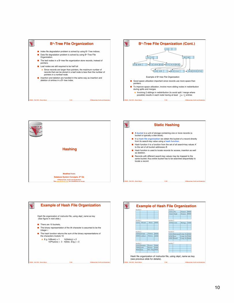
B+-Tree File Organization!
■ Index file degradation problem is solved by using B+-Tree indices.!■ Data file degradation problem is solved by using B+-Tree File
Organization.!■ The leaf nodes in a B+-tree file organization store records, instead of
pointers.!■ Leaf nodes are still required to be half full!
● Since records are larger than pointers, the maximum number of records that can be stored in a leaf node is less than the number of pointers in a nonleaf node.!
■ Insertion and deletion are handled in the same way as insertion and deletion of entries in a B+-tree index.!
©Silberschatz, Korth and Sudarshan!11.56!CS425 – Fall 2013 – Boris Glavic!
B+-Tree File Organization (Cont.)!
■ Good space utilization important since records use more space than pointers. !
■ To improve space utilization, involve more sibling nodes in redistribution during splits and merges!● Involving 2 siblings in redistribution (to avoid split / merge where
possible) results in each node having at least entries!!
Example of B+-tree File Organization!
⎣ ⎦3/2n
Modified from:!Database System Concepts, 6th Ed.!
©Silberschatz, Korth and SudarshanSee www.db-book.com for conditions on re-use !
Hashing!
©Silberschatz, Korth and Sudarshan!11.58!CS425 – Fall 2013 – Boris Glavic!
Static Hashing!
■ A bucket is a unit of storage containing one or more records (a bucket is typically a disk block). !
■ In a hash file organization we obtain the bucket of a record directly from its search-key value using a hash function.!
■ Hash function h is a function from the set of all search-key values K to the set of all bucket addresses B."
■ Hash function is used to locate records for access, insertion as well as deletion.!
■ Records with different search-key values may be mapped to the same bucket; thus entire bucket has to be searched sequentially to locate a record. !
©Silberschatz, Korth and Sudarshan!11.59!CS425 – Fall 2013 – Boris Glavic!
Example of Hash File Organization!
■ There are 10 buckets,!■ The binary representation of the ith character is assumed to be the
integer i.!■ The hash function returns the sum of the binary representations of
the characters modulo 10!● E.g. h(Music) = 1 h(History) = 2
h(Physics) = 3 h(Elec. Eng.) = 3!
Hash file organization of instructor file, using dept_name as key (See figure in next slide.)!
©Silberschatz, Korth and Sudarshan!11.60!CS425 – Fall 2013 – Boris Glavic!
Example of Hash File Organization !
Hash file organization of instructor file, using dept_name as key (see previous slide for details).!
bucket 0
bucket 1
bucket 2
bucket 3
bucket 4
bucket 5
bucket 6
bucket 7
45565
15151 Mozart Music 40000
80000Wu12121 Finance 90000
76543 FinanceSingh
10101 Comp. Sci.SrinivasanKatz Comp. Sci. 75000
92000
650003234358583
El SaidCalifieri
HistoryHistory
8000060000
EinsteinGoldKim
222223345698345
PhysicsPhysicsElec. Eng.
950008700080000
Brandt83821 Comp. Sci.
76766 Crick Biology 72000
11!
©Silberschatz, Korth and Sudarshan!11.61!CS425 – Fall 2013 – Boris Glavic!
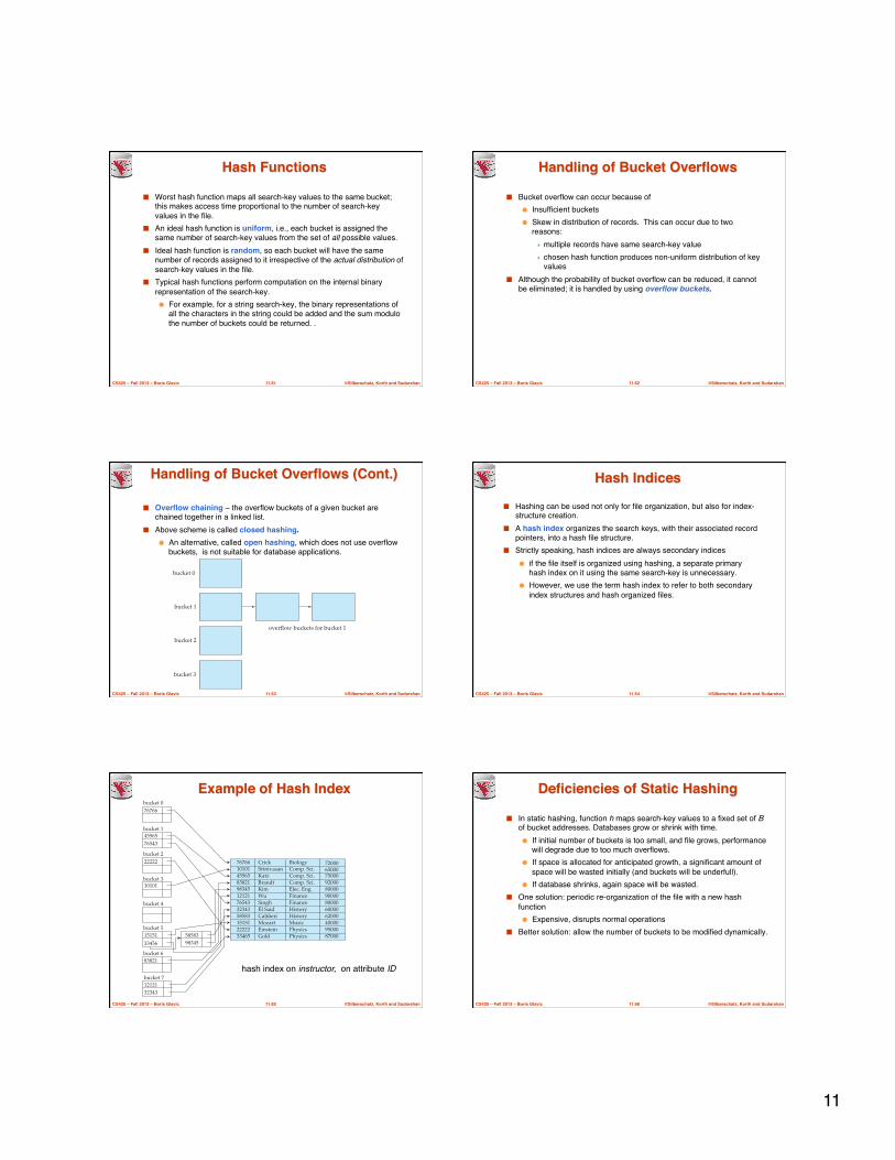
Hash Functions!
■ Worst hash function maps all search-key values to the same bucket; this makes access time proportional to the number of search-key values in the file.!
■ An ideal hash function is uniform, i.e., each bucket is assigned the same number of search-key values from the set of all possible values.!
■ Ideal hash function is random, so each bucket will have the same number of records assigned to it irrespective of the actual distribution of search-key values in the file.!
■ Typical hash functions perform computation on the internal binary representation of the search-key. !● For example, for a string search-key, the binary representations of
all the characters in the string could be added and the sum modulo the number of buckets could be returned. .!
©Silberschatz, Korth and Sudarshan!11.62!CS425 – Fall 2013 – Boris Glavic!
Handling of Bucket Overflows!
■ Bucket overflow can occur because of !● Insufficient buckets !● Skew in distribution of records. This can occur due to two
reasons:!! multiple records have same search-key value!! chosen hash function produces non-uniform distribution of key
values!■ Although the probability of bucket overflow can be reduced, it cannot
be eliminated; it is handled by using overflow buckets.!
©Silberschatz, Korth and Sudarshan!11.63!CS425 – Fall 2013 – Boris Glavic!
Handling of Bucket Overflows (Cont.)!
■ Overflow chaining – the overflow buckets of a given bucket are chained together in a linked list.!
■ Above scheme is called closed hashing. !● An alternative, called open hashing, which does not use overflow
buckets, is not suitable for database applications.!
overflow buckets for bucket 1
bucket 0
bucket 1
bucket 2
bucket 3
©Silberschatz, Korth and Sudarshan!11.64!CS425 – Fall 2013 – Boris Glavic!
Hash Indices!
■ Hashing can be used not only for file organization, but also for index-structure creation. !
■ A hash index organizes the search keys, with their associated record pointers, into a hash file structure.!
■ Strictly speaking, hash indices are always secondary indices !● if the file itself is organized using hashing, a separate primary
hash index on it using the same search-key is unnecessary. !● However, we use the term hash index to refer to both secondary
index structures and hash organized files. !
©Silberschatz, Korth and Sudarshan!11.65!CS425 – Fall 2013 – Boris Glavic!
Example of Hash Index!bucket 0
bucket 1
bucket 2
bucket 3
bucket 4
bucket 5
bucket 6
76766
4556576543
10101
1515133456
58583
83821
22222
98345
bucket 71212132343
76766 Crick
76543 Singh32343 El Said58583 Califieri15151 Mozart22222 Einstein33465 Gold
10101 Srinivasan45565 Katz83821 Brandt98345 Kim12121 Wu
Biology
Physics
FinanceHistoryHistoryMusic
Physics
Comp. Sci.Comp. Sci.Comp. Sci.Elec. Eng.Finance
72000
800006000062000400009500087000
6500075000920008000090000
hash index on instructor, on attribute ID!
©Silberschatz, Korth and Sudarshan!11.66!CS425 – Fall 2013 – Boris Glavic!
Deficiencies of Static Hashing!
■ In static hashing, function h maps search-key values to a fixed set of B of bucket addresses. Databases grow or shrink with time. !● If initial number of buckets is too small, and file grows, performance
will degrade due to too much overflows.!● If space is allocated for anticipated growth, a significant amount of
space will be wasted initially (and buckets will be underfull).!● If database shrinks, again space will be wasted.!
■ One solution: periodic re-organization of the file with a new hash function!● Expensive, disrupts normal operations!
■ Better solution: allow the number of buckets to be modified dynamically. !

12!
©Silberschatz, Korth and Sudarshan!11.67!CS425 – Fall 2013 – Boris Glavic!
Index Definition in SQL!
■ Create an index!! !create index <index-name> on <relation-name>
! ! !(<attribute-list>)!E.g.: create index b-index on branch(branch_name)!
■ Use create unique index to indirectly specify and enforce the condition that the search key is a candidate key is a candidate key.!● Not really required if SQL unique integrity constraint is supported!
■ To drop an index !! ! !drop index <index-name>!
■ Most database systems allow specification of type of index, and clustering.!
Modified from:!Database System Concepts, 6th Ed.!
©Silberschatz, Korth and SudarshanSee www.db-book.com for conditions on re-use !
End of Chapter!
©Silberschatz, Korth and Sudarshan!11.69!CS425 – Fall 2013 – Boris Glavic!
Figure 11.01!10101 Srinivasan
45565 Katz58583 Califieri76543 Singh76766 Crick83821 Brandt98345 Kim
12121 Wu15151 Mozart22222 Einstein32343 El Said33456 Gold
Comp. Sci.
Comp. Sci.
Comp. Sci.HistoryFinanceBiology
Elec. Eng.
FinanceMusicPhysicsHistoryPhysics
65000
750006200080000720009200080000
9000040000950006000087000
©Silberschatz, Korth and Sudarshan!11.70!CS425 – Fall 2013 – Boris Glavic!
Figure 11.15 !
©Silberschatz, Korth and Sudarshan!11.71!CS425 – Fall 2013 – Boris Glavic!
Partitioned Hashing!
■ Hash values are split into segments that depend on each attribute of the search-key.!! !(A1, A2, . . . , An) for n attribute search-key!
■ Example: n = 2, for customer, search-key being (customer-street, customer-city)!! !search-key value "hash value
"(Main, Harrison) !101 111 !(Main, Brooklyn) !101 001 !(Park, Palo Alto) !010 010 !(Spring, Brooklyn) !001 001 !(Alma, Palo Alto) !110 010!
■ To answer equality query on single attribute, need to look up multiple buckets. Similar in effect to grid files. !
©Silberschatz, Korth and Sudarshan!11.72!CS425 – Fall 2013 – Boris Glavic!
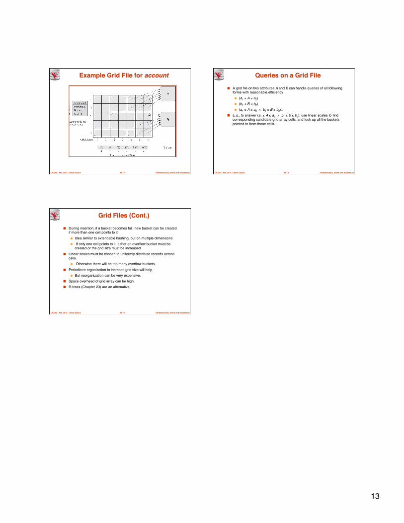
Grid Files!
■ Structure used to speed the processing of general multiple search-key queries involving one or more comparison operators.!
■ The grid file has a single grid array and one linear scale for each search-key attribute. The grid array has number of dimensions equal to number of search-key attributes.!
■ Multiple cells of grid array can point to same bucket!■ To find the bucket for a search-key value, locate the row and column
of its cell using the linear scales and follow pointer!
13!
©Silberschatz, Korth and Sudarshan!11.73!CS425 – Fall 2013 – Boris Glavic!
Example Grid File for account!
©Silberschatz, Korth and Sudarshan!11.74!CS425 – Fall 2013 – Boris Glavic!
Queries on a Grid File!
■ A grid file on two attributes A and B can handle queries of all following forms with reasonable efficiency !● (a1 ≤ A ≤ a2)!● (b1 ≤ B ≤ b2)!● (a1 ≤ A ≤ a2 ∧ b1 ≤ B ≤ b2),.!
■ E.g., to answer (a1 ≤ A ≤ a2 ∧ b1 ≤ B ≤ b2), use linear scales to find corresponding candidate grid array cells, and look up all the buckets pointed to from those cells.!
©Silberschatz, Korth and Sudarshan!11.75!CS425 – Fall 2013 – Boris Glavic!
Grid Files (Cont.)!
■ During insertion, if a bucket becomes full, new bucket can be created if more than one cell points to it. !● Idea similar to extendable hashing, but on multiple dimensions!● If only one cell points to it, either an overflow bucket must be
created or the grid size must be increased!■ Linear scales must be chosen to uniformly distribute records across
cells. !● Otherwise there will be too many overflow buckets.!
■ Periodic re-organization to increase grid size will help.!● But reorganization can be very expensive.!
■ Space overhead of grid array can be high.!■ R-trees (Chapter 23) are an alternative !