DBMS Internal Review. Outline Storage and Indexing Query Optimization.
74
DBMS Internal Review
-
Upload
marjorie-gilbert -
Category
Documents
-
view
228 -
download
0
Transcript of DBMS Internal Review. Outline Storage and Indexing Query Optimization.
DBMS InternalReview
Outline
• Storage and Indexing
• Query Optimization
Overview of Storage and Indexing
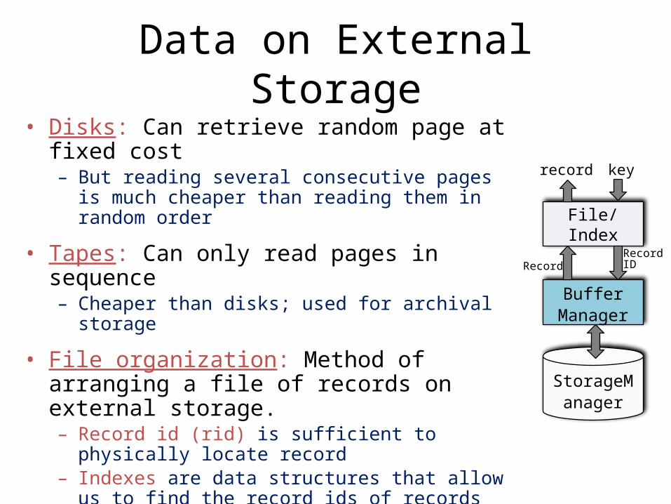
Data on External Storage• Disks: Can retrieve random page at fixed cost
– But reading several consecutive pages is much cheaper than reading them in random order
• Tapes: Can only read pages in sequence– Cheaper than disks; used for archival storage
• File organization: Method of arranging a file of records on external storage.– Record id (rid) is sufficient to physically locate record– Indexes are data structures that allow us to find the record
ids of records with given values in index search key fields
• Architecture: Buffer manager stages pages from external storage to main memory buffer pool. – File and index layers make calls to the buffer manager.
StorageManager
Buffer Manager
RecordID
File/Index
keyrecord
Record
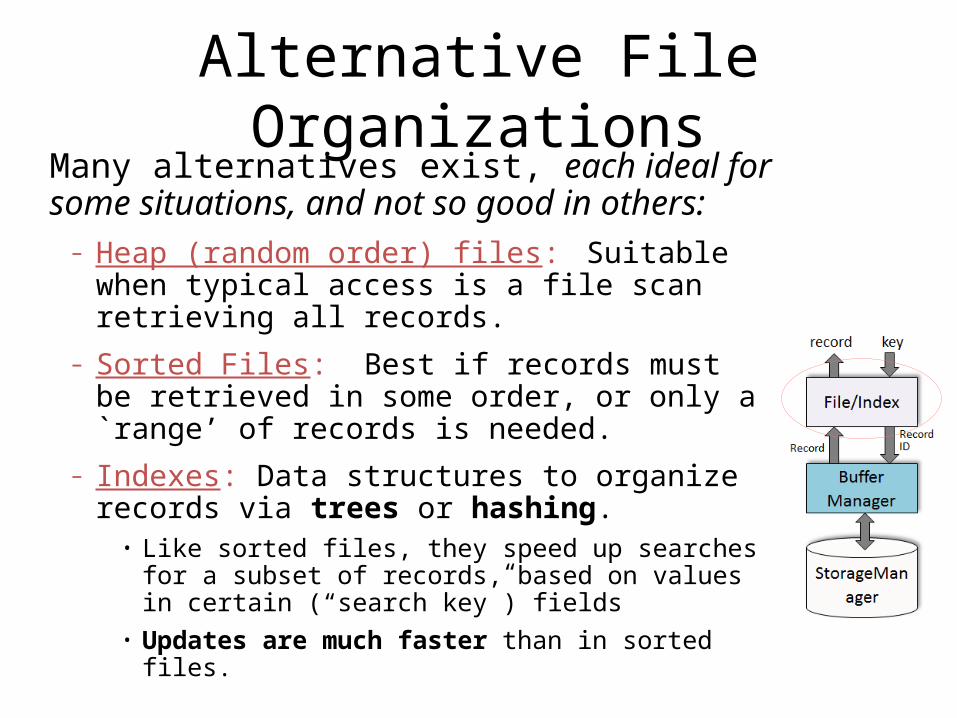
Alternative File OrganizationsMany alternatives exist, each ideal for some situations, and not so good in others:– Heap (random order) files: Suitable when
typical access is a file scan retrieving all records.– Sorted Files: Best if records must be retrieved in
some order, or only a `range’ of records is needed.
– Indexes: Data structures to organize records via trees or hashing. • Like sorted files, they speed up searches for a subset
of records, based on values in certain (“search key”) fields
• Updates are much faster than in sorted files.
Indexes – Search Key
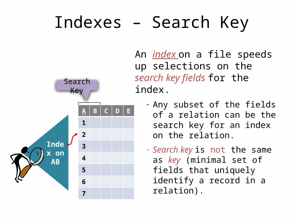
An index on a file speeds up selections on the search key fields for the index.
– Any subset of the fields of a relation can be the search key for an index on the relation.
– Search key is not the same as key (minimal set of fields that uniquely identify a record in a relation).
A B C D E
1
2
3
4
5
6
7
Index on AB
Search Key
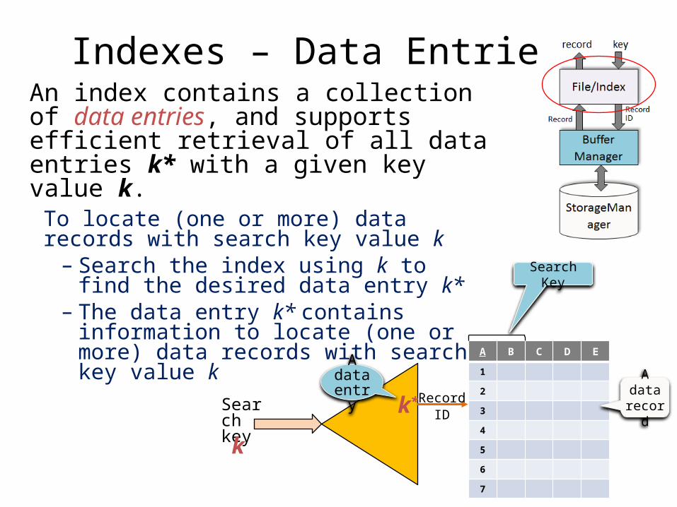
Indexes – Data Entries An index contains a collection of data entries, and supports efficient retrieval of all data entries k* with a given key value k.
To locate (one or more) data records with search key value k– Search the index using k to find the
desired data entry k*– The data entry k* contains
information to locate (one or more) data records with search key value k
A B C D E
1
2
3
4
5
6
7
Search Key
Search key
Record ID
k
k*A data record
A data entry
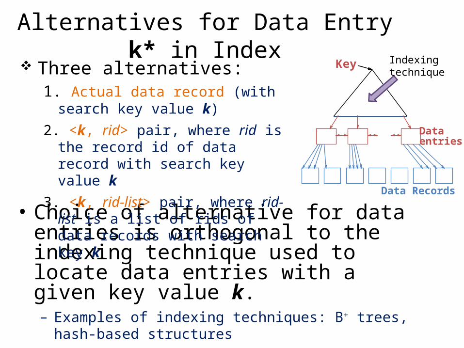
Alternatives for Data Entry k* in Index
• Choice of alternative for data entries is orthogonal to the indexing technique used to locate data entries with a given key value k.– Examples of indexing techniques: B+ trees, hash-based structures– Typically, index contains auxiliary information that directs
searches to the desired data entries
Three alternatives:1. Actual data record (with search key
value k)2. <k, rid> pair, where rid is the record id
of data record with search key value k3. <k, rid-list> pair, where rid-list is a list of
rids of data records with search key k
Dataentries
Data Records
Key Indexingtechnique
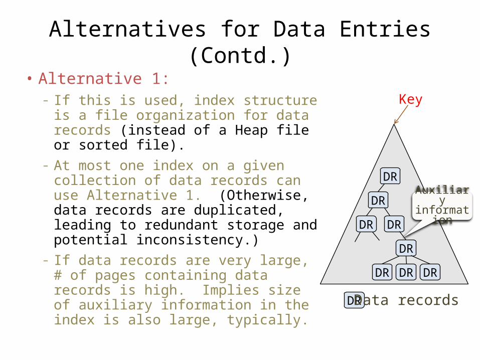
Alternatives for Data Entries (Contd.)• Alternative 1:
– If this is used, index structure is a file organization for data records (instead of a Heap file or sorted file).
– At most one index on a given collection of data records can use Alternative 1. (Otherwise, data records are duplicated, leading to redundant storage and potential inconsistency.)
– If data records are very large, # of pages containing data records is high. Implies size of auxiliary information in the index is also large, typically.
DR
DR
DRDR
DR
DR DR DR
Key
DR Data records
Auxiliaryinformation
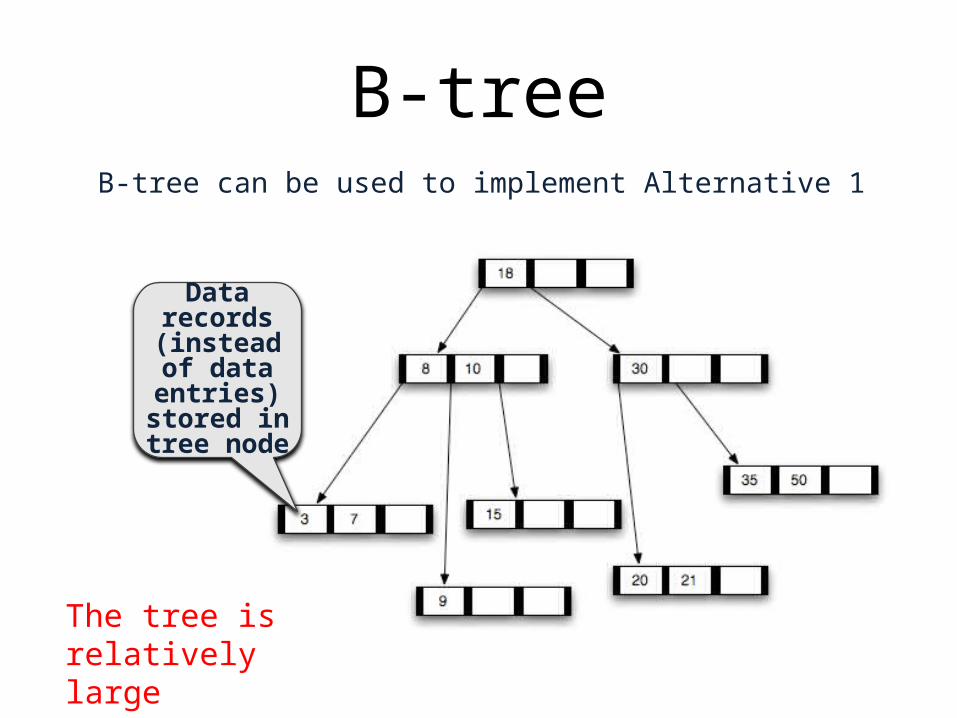
B-treeB-tree can be used to implement Alternative 1
Data records (instead of
data entries) stored intree node
The tree is relatively large
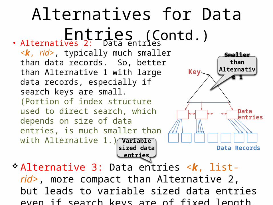
Variable sized data entries
Alternatives for Data Entries (Contd.)• Alternatives 2: Data entries <k, rid>,
typically much smaller than data records. So, better than Alternative 1 with large data records, especially if search keys are small. (Portion of index structure used to direct search, which depends on size of data entries, is much smaller than with Alternative 1.)
Dataentries
Data Records
Key
Alternative 3: Data entries <k, list-rid>, more compact than Alternative 2, but leads to variable sized data entries even if search keys are of fixed length.
Smaller than Alternative 1
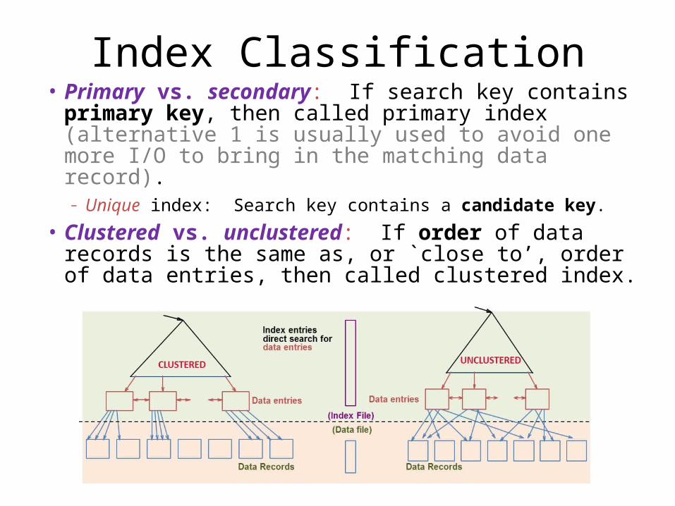
Index Classification• Primary vs. secondary: If search key contains
primary key, then called primary index (alternative 1 is usually used to avoid one more I/O to bring in the matching data record).– Unique index: Search key contains a candidate key.
• Clustered vs. unclustered: If order of data records is the same as, or `close to’, order of data entries, then called clustered index.

Clustered IndexSuppose that Alternative (2) is used for data entries, and that the data records are stored in a Heap file.– To build clustered index, first sort the Heap file (with some
free space on each page for future inserts). – Overflow pages may be needed for inserts. (Thus, order of
data records is `close to’, but not identical to, the sort order.)
Index entries
Data entries
direct search for
(Index File)
(Data file)
Data Records
data entries
CLUSTERED
Heap file
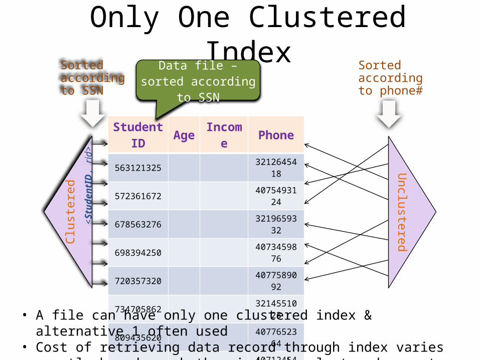
Only One Clustered Index
StudentID Age Income Phone
563121325 3212645418
572361672 4075493124
678563276 3219659332
698394250 4073459876
720357320 4077589092
734705862 3214551023
809435620 4077652364
903429554 4071245436
Sortedaccordingto SSN
Clus
tere
dSortedaccordingto phone#
Unclustered
Data file – sorted according to SSN
<Stu
dent
ID, r
id>
• A file can have only one clustered index & alternative 1 often used• Cost of retrieving data record through index varies greatly based on whether
index is clustered or not
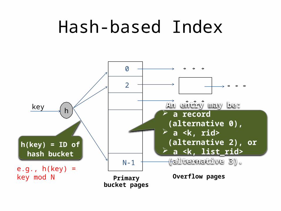
Hash-based Index
h
e.g., h(key) = key mod N
key
Primarybucket pages
Overflow pages
2
0
N-1
h(key) = ID of hash bucket
An entry may be: a record (alternative 0), a <k, rid> (alternative 2), or a <k, list_rid> (alternative 3).
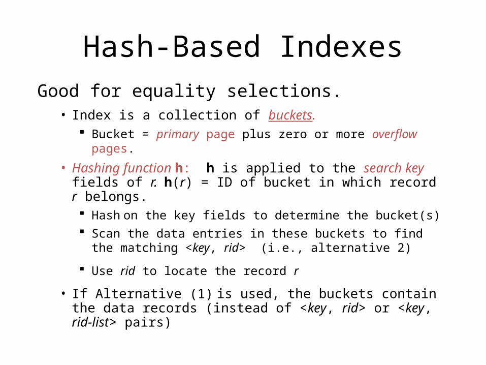
Hash-Based IndexesGood for equality selections.
• Index is a collection of buckets. Bucket = primary page plus zero or more overflow pages.
• Hashing function h: h is applied to the search key fields of r. h(r) = ID of bucket in which record r belongs. Hash on the key fields to determine the bucket(s) Scan the data entries in these buckets to find the
matching <key, rid> (i.e., alternative 2)
Use rid to locate the record r
• If Alternative (1) is used, the buckets contain the data records (instead of <key, rid> or <key, rid-list> pairs)
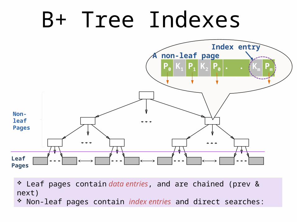
B+ Tree Indexes
Non-leaf Pages
Leaf Pages
P0 K1 P1 K2 P0 . . . Km Pm
Index entryA non-leaf page
Leaf pages contain data entries, and are chained (prev & next) Non-leaf pages contain index entries and direct searches:
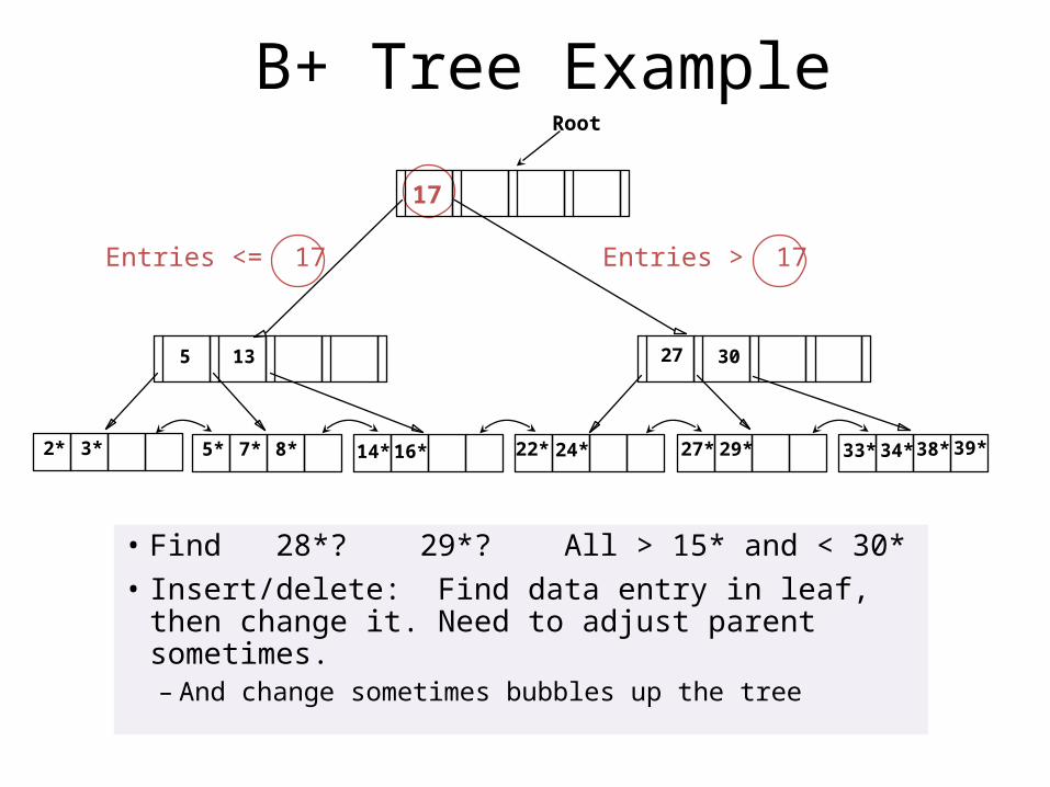
B+ Tree Example
• Find 28*? 29*? All > 15* and < 30*• Insert/delete: Find data entry in leaf, then
change it. Need to adjust parent sometimes.– And change sometimes bubbles up the tree
2* 3*
Root
17
30
14* 16* 33* 34* 38* 39*
135
7*5* 8* 22* 24*
27
27* 29*
Entries <= 17 Entries > 17
Choice of Indexes
• What indexes should we create?– Which relations should have indexes? – What field(s) should be the search key? – Should we build several indexes?
• For each index, what kind of an index should it be?– Clustered? – Hash/tree?
Choice of Indexes (Contd.)• One approach: – Consider the most important queries in turn.– Consider the best plan using the current indexes,
and see if a better plan is possible with an additional index. If so, create it.→ Obviously, this implies that we must understand how
a DBMS evaluates queries and creates query evaluation plans!
• Before creating an index, must also consider the impact on updates in the workload!– Trade-off: Indexes can make queries go faster, updates
slower. Require disk space, too.
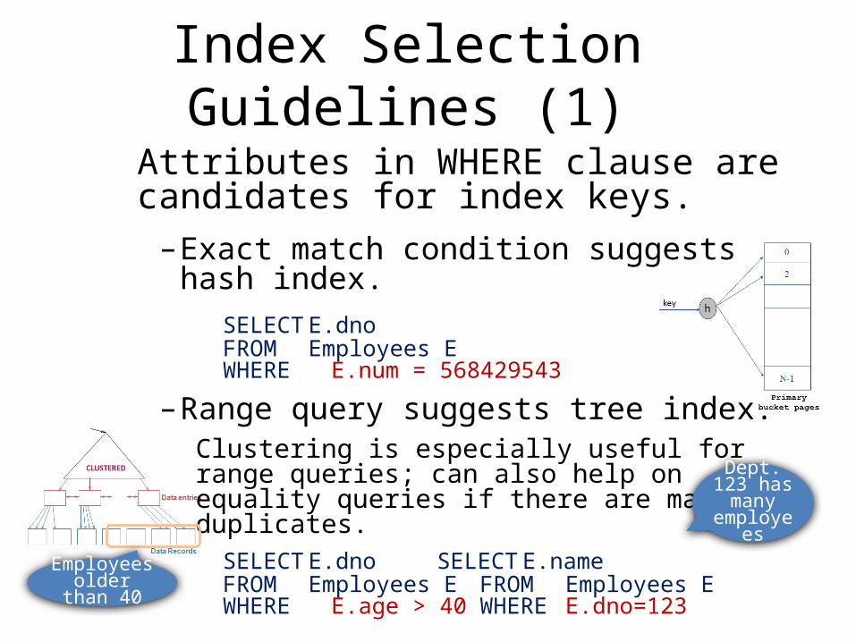
Index Selection Guidelines (1)
Attributes in WHERE clause are candidates for index keys.–Exact match condition suggests hash index.
SELECT E.dnoFROM Employees EWHERE E.num = 568429543
–Range query suggests tree index.Clustering is especially useful for range queries; can also help on equality queries if there are many duplicates.
SELECT E.dno SELECT E.nameFROM Employees E FROM Employees EWHERE E.age > 40 WHERE E.dno=123
Dept. 123 has many
employees
Employees older than 40
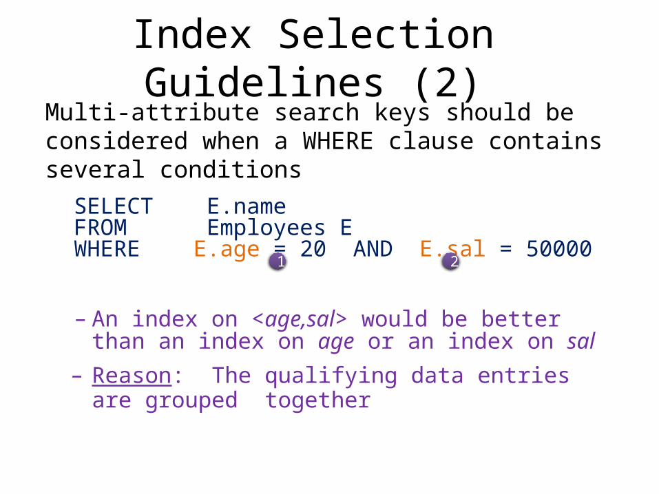
Index Selection Guidelines (2)Multi-attribute search keys should be considered when a WHERE clause contains several conditions
SELECT E.nameFROM Employees EWHERE E.age = 20 AND E.sal = 50000
– An index on <age,sal> would be better than an index on age or an index on sal
– Reason: The qualifying data entries are grouped together
1 2
Index Selection Guidelines (3)
• Indexes can sometimes enable index-only evaluation for important queries.
Example: use leaf pages of index on age to compute the average age
• Try to choose indexes that benefit as many queries as possible.
• Since only one index can be clustered per relation, choose it based on important queries that would benefit the most from clustering.
On age
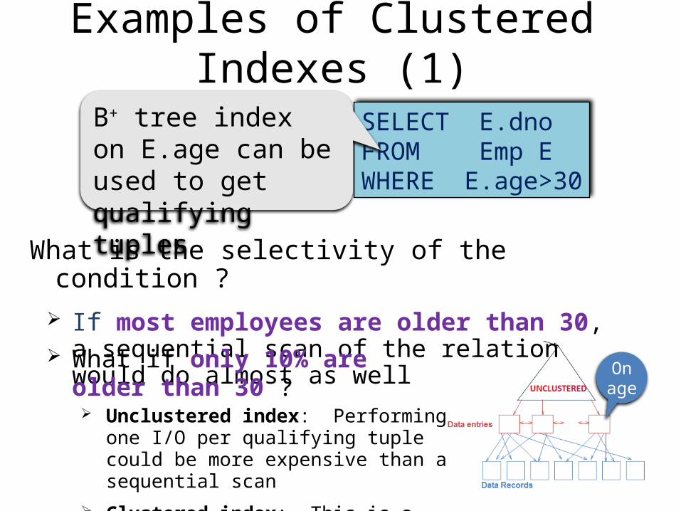
Examples of Clustered Indexes (1)
What is the selectivity of the condition ? If most employees are older than 30, a sequential
scan of the relation would do almost as well
SELECT E.dnoFROM Emp EWHERE E.age>30
B+ tree index on E.age can be used to get qualifying tuples
What if only 10% are older than 30 ? Unclustered index: Performing one I/O per
qualifying tuple could be more expensive than a sequential scan
Clustered index: This is a good option
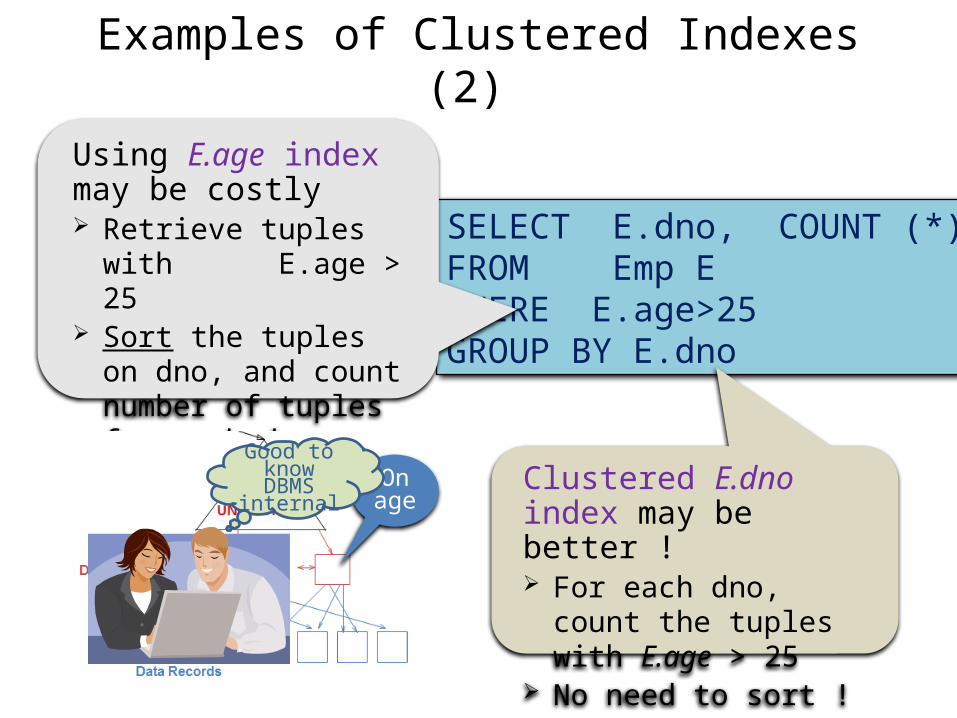
Examples of Clustered Indexes (2)
SELECT E.dno, COUNT (*)FROM Emp EWHERE E.age>25GROUP BY E.dno
Clustered E.dno index may be better ! For each dno, count the
tuples with E.age > 25 No need to sort !
Using E.age index may be costly Retrieve tuples with
E.age > 25 Sort the tuples on dno,
and count number of tuples for each dno
On age
Good to know DBMS
internal
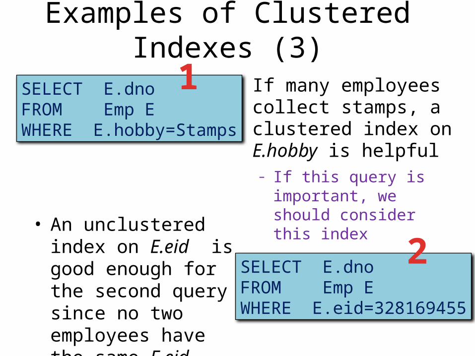
Examples of Clustered Indexes (3)
• If many employees collect stamps, a clustered index on E.hobby is helpful – If this query is important, we
should consider this index
SELECT E.dnoFROM Emp EWHERE E.hobby=Stamps
SELECT E.dnoFROM Emp EWHERE E.eid=328169455
• An unclustered index on E.eid is good enough for the second query since no two employees have the same E.eid.
1
2
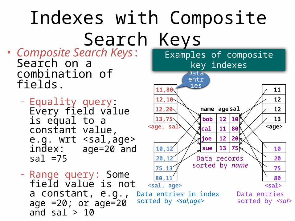
Indexes with Composite Search Keys • Composite Search Keys:
Search on a combination of fields.– Equality query: Every field
value is equal to a constant value, e.g. wrt <sal,age> index: age=20 and sal =75
– Range query: Some field value is not a constant, e.g., age =20; or age=20 and sal > 10
• Data entries in index sorted by search key to support range queries. Data entries in index
sorted by <sal,age>Data entriessorted by <sal>
sue 13 75
bob
cal
joe 12
10
20
8011
12
name age sal
<sal, age>
<age, sal> <age>
<sal>
12,20
12,10
11,80
13,75
20,12
10,12
75,13
80,11
11
12
12
13
10
20
75
80
Data recordssorted by name
Examples of composite key indexes
Data entries
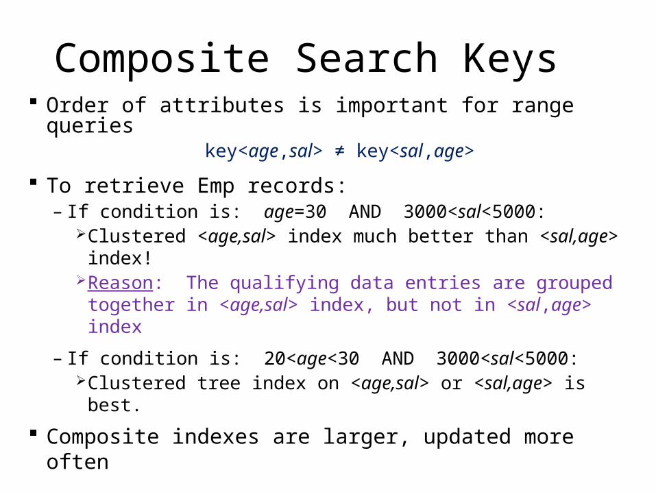
Composite Search Keys Order of attributes is important for range queries
key<age,sal> ≠ key<sal,age>
To retrieve Emp records: – If condition is: age=30 AND 3000<sal<5000:
Clustered <age,sal> index much better than <sal,age> index!
Reason: The qualifying data entries are grouped together in <age,sal> index, but not in <sal,age> index
– If condition is: 20<age<30 AND 3000<sal<5000: Clustered tree index on <age,sal> or <sal,age> is best.
Composite indexes are larger, updated more often
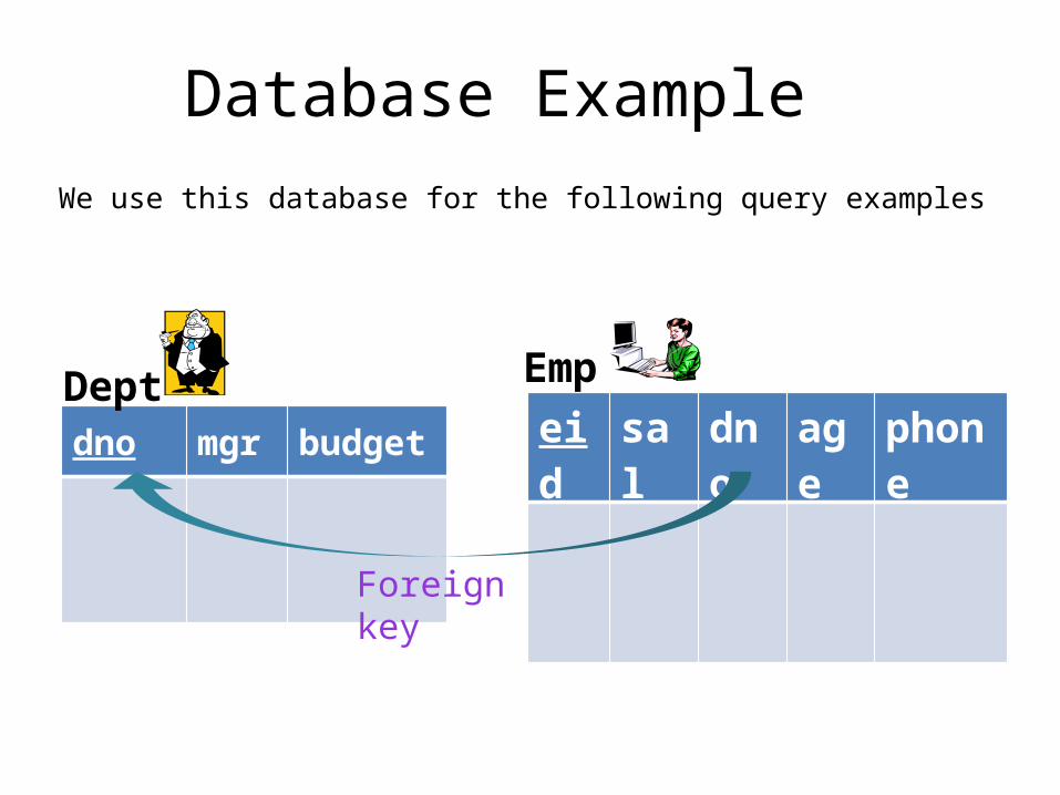
Database Example
We use this database for the following query examples
dno mgr budgetDept
eid sal dno age phone
Emp
Foreign key
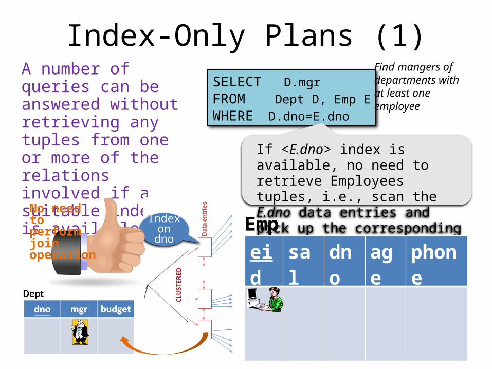
Index-Only Plans (1)A number of queries can be answered without retrieving any tuples from one or more of the relations involved if a suitable index is available.
SELECT D.mgrFROM Dept D, Emp EWHERE D.dno=E.dno
Find mangers of departments with at least one employee
Index on dno
If <E.dno> index is available, no need to retrieve Employees tuples, i.e., scan the E.dno data entries and pick up the corresponding Dept tuples
eid sal dno age phone
EmpNo need to perform join operation
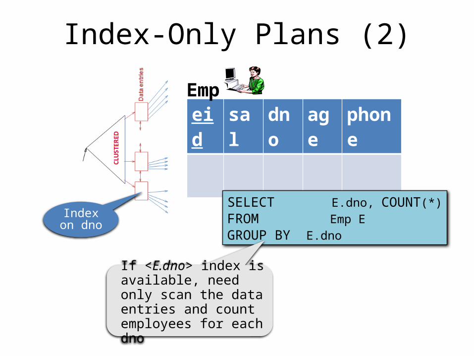
Index-Only Plans (2)
eid sal dno age phoneEmp
Index on dno
SELECT E.dno, COUNT(*)FROM Emp EGROUP BY E.dno
If <E.dno> index is available, need only scan the data entries and count employees for each dno
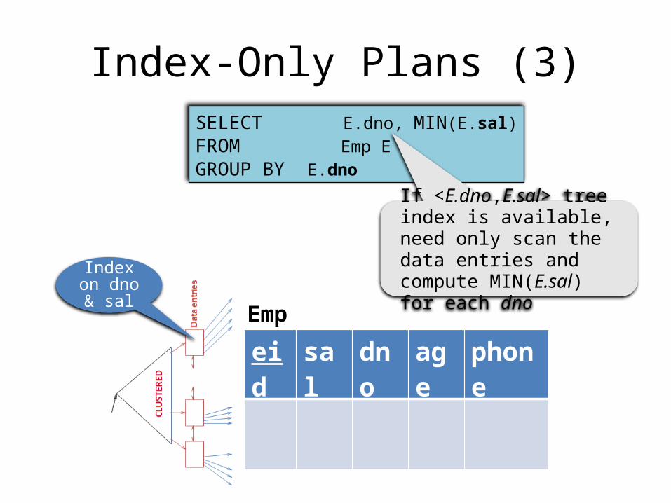
Index-Only Plans (3)SELECT E.dno, MIN(E.sal)FROM Emp EGROUP BY E.dno
If <E.dno,E.sal> tree index is available, need only scan the data entries and compute MIN(E.sal) for each dno
Emp
eid sal dno age phone
Index on dno & sal
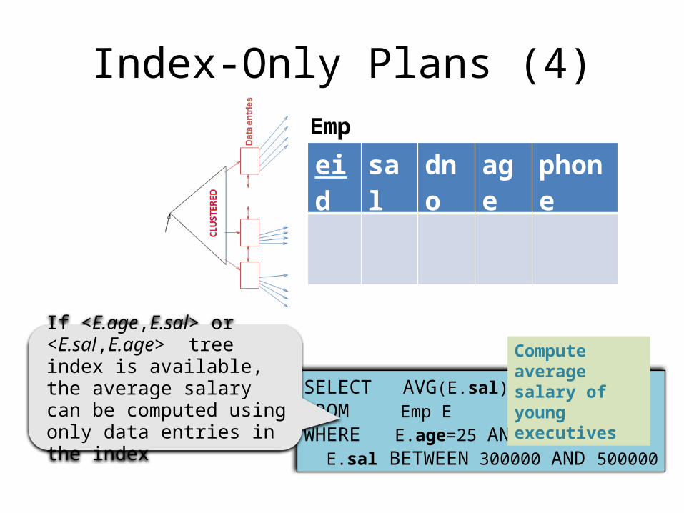
Index-Only Plans (4)
SELECT AVG(E.sal)FROM Emp EWHERE E.age=25 AND E.sal BETWEEN 300000 AND 500000
If <E.age,E.sal> or <E.sal,E.age> tree index is available, the average salary can be computed using only data entries in the index
Emp
eid sal dno age phone
Compute averagesalary of young executives
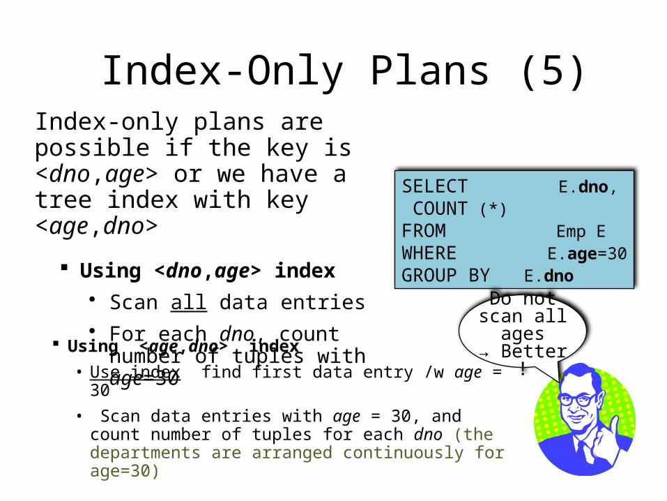
Index-Only Plans (5)
Using <age,dno> index• Use index find first data entry /w age = 30• Scan data entries with age = 30, and count
number of tuples for each dno (the departments are arranged continuously for age=30)
SELECT E.dno, COUNT (*)FROM Emp EWHERE E.age=30GROUP BY E.dno
Index-only plans are possible if the key is <dno,age> or we have a tree index with key <age,dno>
Using <dno,age> index• Scan all data entries• For each dno, count number of
tuples with age=30Do not scan
all ages→ Better !
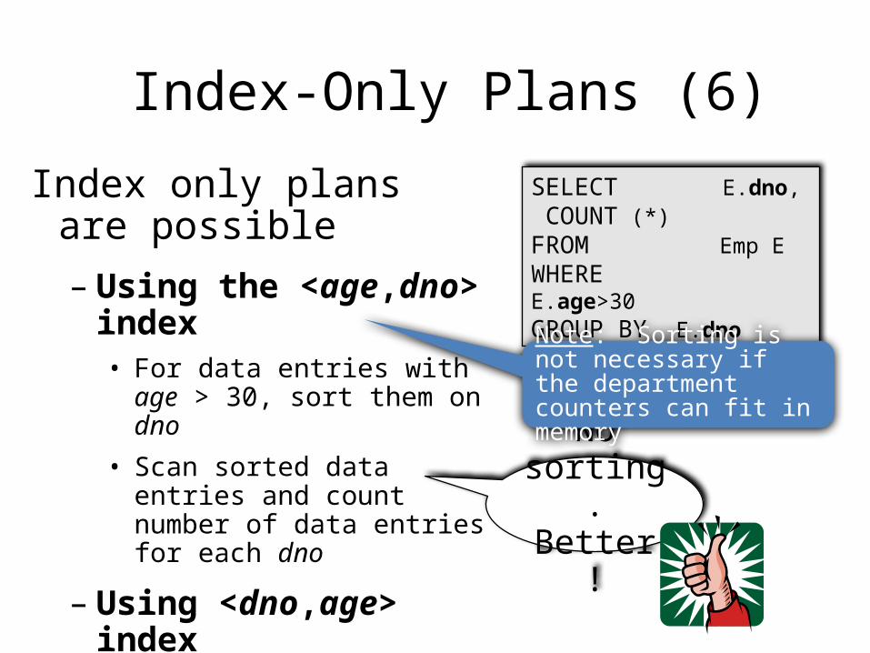
Index-Only Plans (6)
Index only plans are possible – Using the <age,dno> index• For data entries with age > 30,
sort them on dno• Scan sorted data entries and
count number of data entries for each dno
– Using <dno,age> index • Scan data entries• For each dno, count number of
data entries with age > 30
SELECT E.dno, COUNT (*)FROM Emp EWHERE E.age>30GROUP BY E.dno
No sorting. Better !
Note: Sorting is not necessary if the department counters can fit in memory
Summary• Many alternative file organizations exist, each
appropriate in some situation.
• If selection queries are frequent, sorting the file or building an index is important.– Hash-based indexes only good for equality search.– Sorted files and tree-based indexes best for range
search; also good for equality search. (Files rarely kept sorted in practice; B+ tree index is better.)
• Index is a collection of data entries (<key, rid> pairs or <key, rid-list> pairs) plus a way to quickly find entries (using hashing or a search tree) with given key values.
Summary (Contd.)
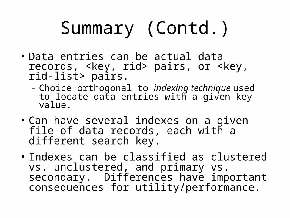
• Data entries can be actual data records, <key, rid> pairs, or <key, rid-list> pairs.– Choice orthogonal to indexing technique used to
locate data entries with a given key value.
• Can have several indexes on a given file of data records, each with a different search key.
• Indexes can be classified as clustered vs. unclustered, and primary vs. secondary. Differences have important consequences for utility/performance.
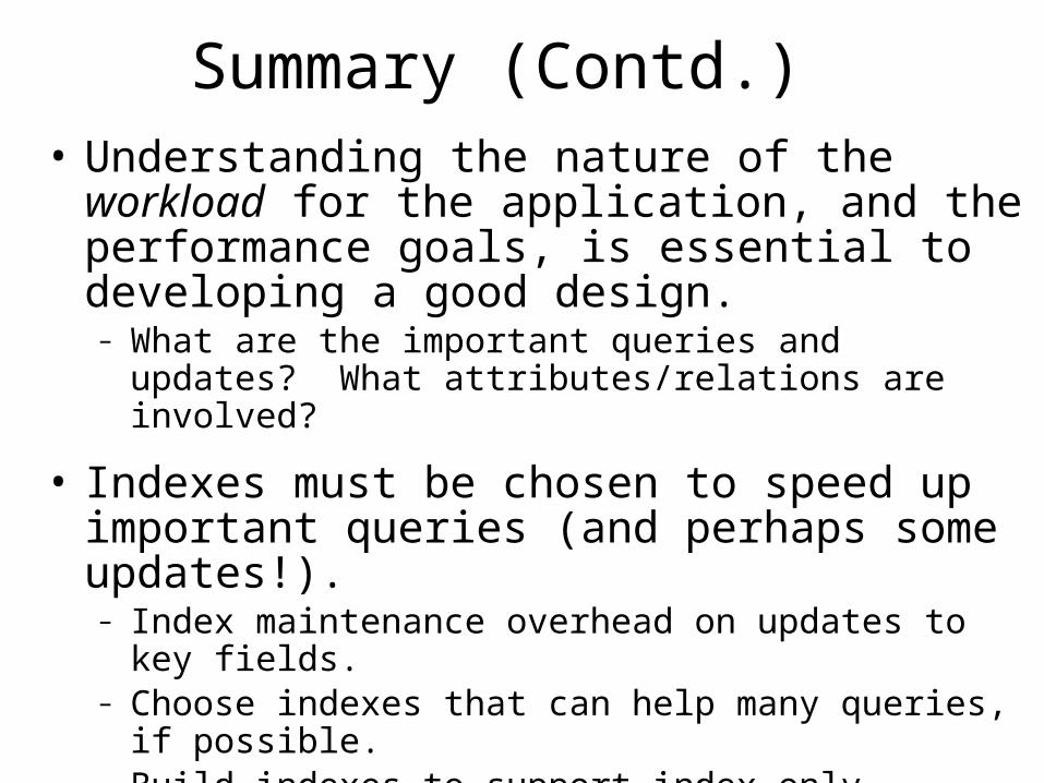
Summary (Contd.)• Understanding the nature of the workload for the
application, and the performance goals, is essential to developing a good design.– What are the important queries and updates? What
attributes/relations are involved?
• Indexes must be chosen to speed up important queries (and perhaps some updates!).– Index maintenance overhead on updates to key fields.– Choose indexes that can help many queries, if possible.– Build indexes to support index-only strategies.– Clustering is an important decision; only one index on a given
relation can be clustered!– Order of fields in composite index key can be important.

Overview of Query Optimization
Internal Query Representation
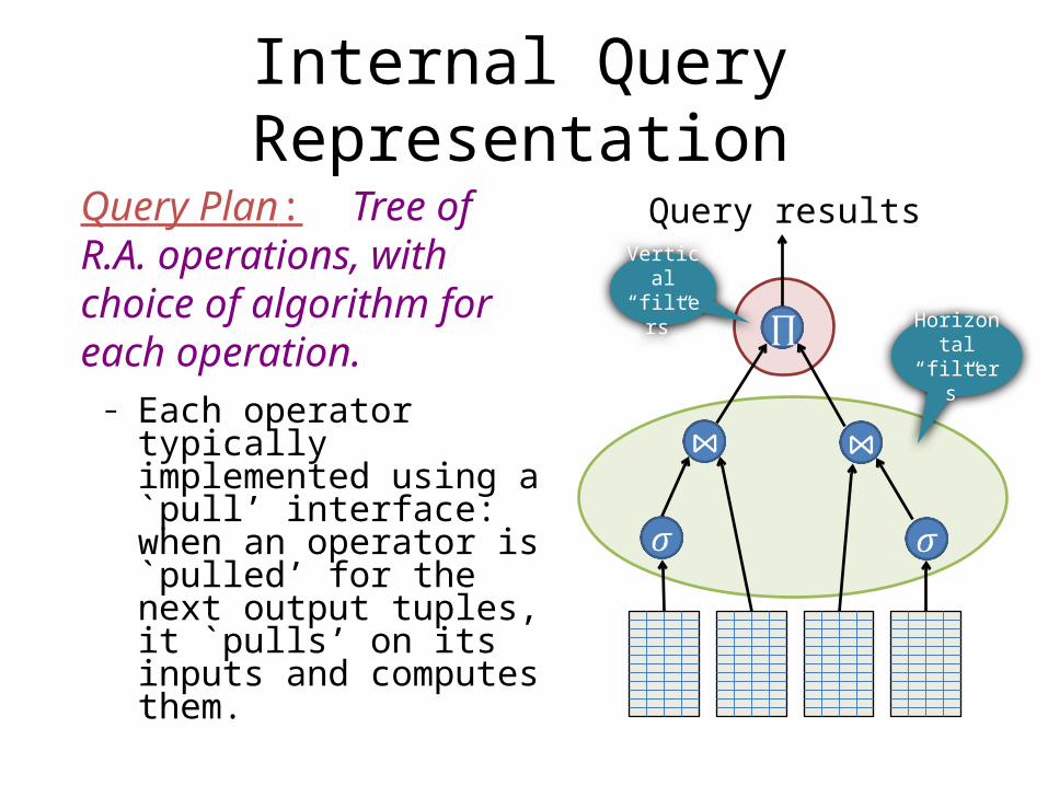
Query Plan: Tree of R.A. operations, with choice of algorithm for each operation.– Each operator typically
implemented using a `pull’ interface: when an operator is `pulled’ for the next output tuples, it `pulls’ on its inputs and computes them.
Query results
Horizontal “filters”
Vertical “filters”
Overview of Query Evaluation
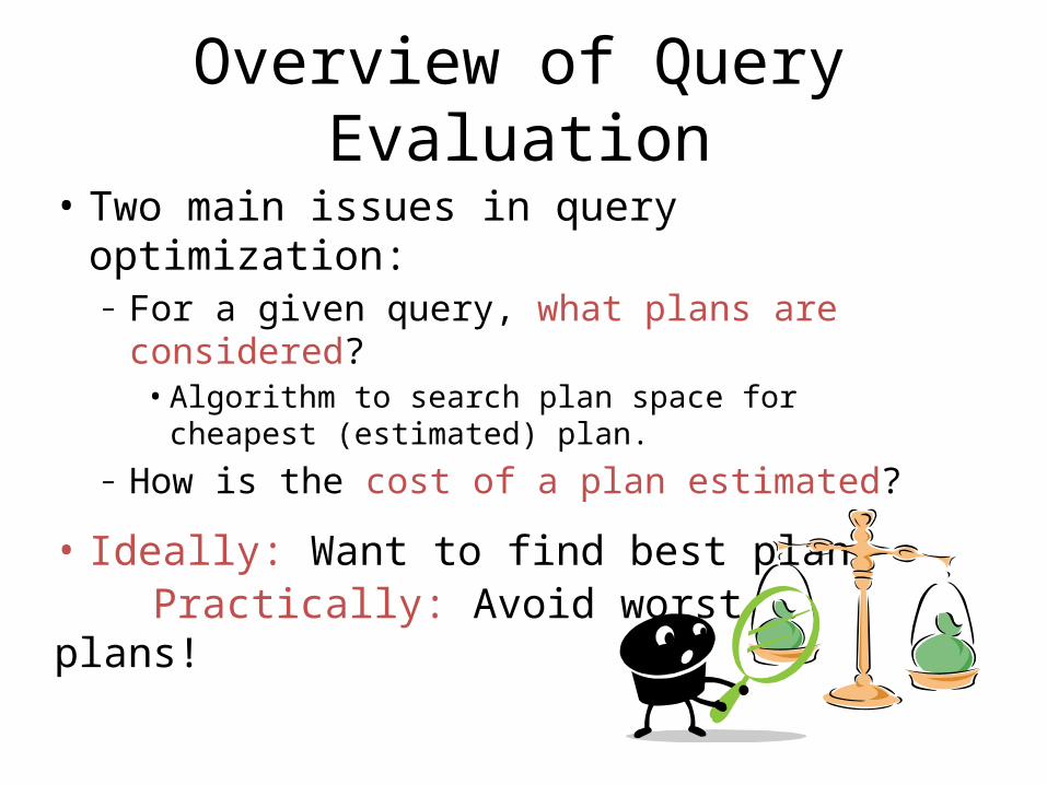
• Two main issues in query optimization:– For a given query, what plans are considered?• Algorithm to search plan space for cheapest
(estimated) plan.– How is the cost of a plan estimated?
• Ideally: Want to find best plan. Practically: Avoid worst plans!
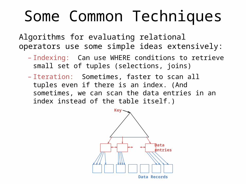
Some Common TechniquesAlgorithms for evaluating relational operators use some simple ideas extensively:– Indexing: Can use WHERE conditions to retrieve small
set of tuples (selections, joins)
– Iteration: Sometimes, faster to scan all tuples even if there is an index. (And sometimes, we can scan the data entries in an index instead of the table itself.)
Dataentries
Data Records
Key
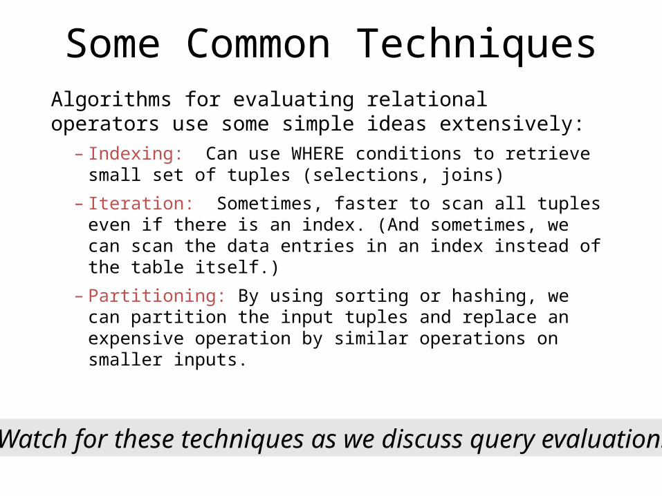
Some Common TechniquesAlgorithms for evaluating relational operators use some simple ideas extensively:– Indexing: Can use WHERE conditions to retrieve
small set of tuples (selections, joins)
– Iteration: Sometimes, faster to scan all tuples even if there is an index. (And sometimes, we can scan the data entries in an index instead of the table itself.)
– Partitioning: By using sorting or hashing, we can partition the input tuples and replace an expensive operation by similar operations on smaller inputs.
Watch for these techniques as we discuss query evaluation!
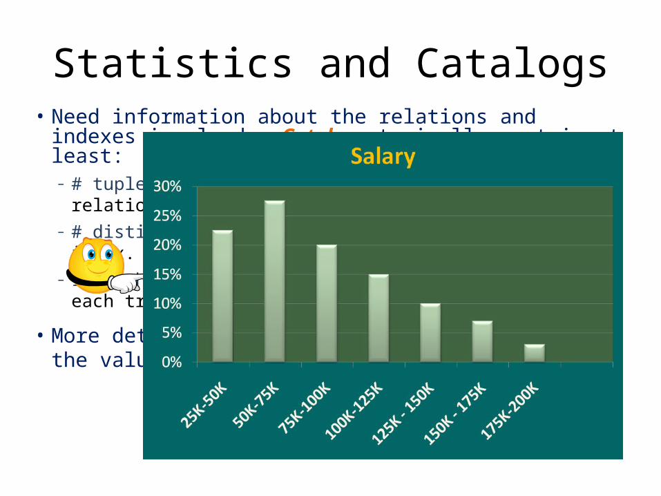
Statistics and Catalogs• Need information about the relations and indexes
involved. Catalogs typically contain at least:– # tuples (NTuples) and # pages (NPages) for each
relation.– # distinct key values (NKeys) and NPages for each index.– Index height, low/high key values (Low/High) for each
tree index.
• More detailed information (e.g., histograms of the values in some field) are sometimes stored.
Avoid using unclustered index in
this range
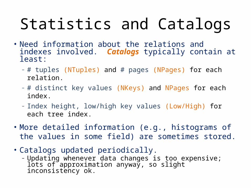
Statistics and Catalogs• Need information about the relations and indexes
involved. Catalogs typically contain at least:– # tuples (NTuples) and # pages (NPages) for each relation.– # distinct key values (NKeys) and NPages for each index.– Index height, low/high key values (Low/High) for each
tree index.
• More detailed information (e.g., histograms of the values in some field) are sometimes stored.
• Catalogs updated periodically.– Updating whenever data changes is too expensive; lots of
approximation anyway, so slight inconsistency ok.
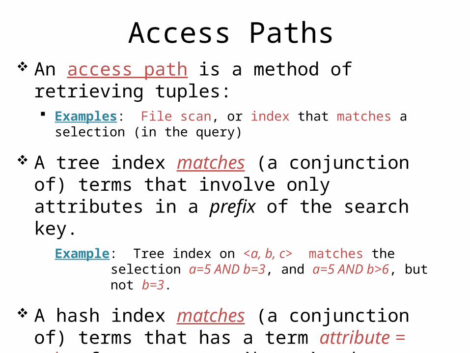
Access Paths An access path is a method of retrieving tuples:
Examples: File scan, or index that matches a selection (in the query)
A tree index matches (a conjunction of) terms that involve only attributes in a prefix of the search key.
Example: Tree index on <a, b, c> matches the selection a=5 AND b=3, and a=5 AND b>6, but not b=3.
A hash index matches (a conjunction of) terms that has a term attribute = value for every attribute in the search key of the index.
Example: Hash index on <a, b, c> matches a=5 AND b=3 AND c=5; but it does not match b=3, or a=5 AND b=3, or a>5 AND b=3 AND c=5.
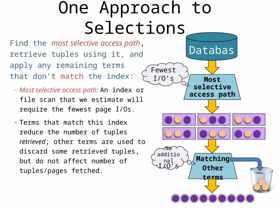
One Approach to SelectionsFind the most selective access path, retrieve tuples using it, and apply any remaining terms that don’t match the index:
– Most selective access path: An index or file scan that we estimate will require the fewest page I/Os.
– Terms that match this index reduce the number of tuples retrieved; other terms are used to discard some retrieved tuples, but do not affect number of tuples/pages fetched.
Database
Most selective access path
Matching Other terms
Fewest I/O’s
No additional
I/O’s
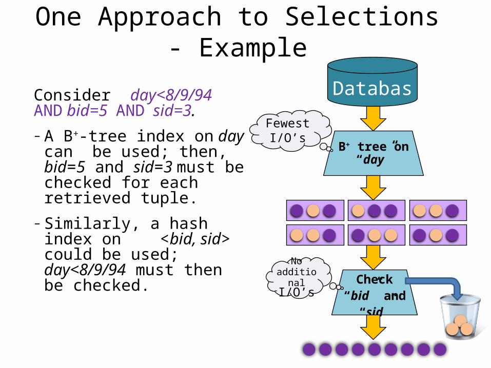
One Approach to Selections - Example
Consider day<8/9/94 AND bid=5 AND sid=3. – A B+-tree index on day can
be used; then, bid=5 and sid=3 must be checked for each retrieved tuple.
– Similarly, a hash index on <bid, sid> could be used; day<8/9/94 must then be checked.
Database
B+ tree on“day”
Check “bid” and “sid”
Fewest I/O’s
No additional
I/O’s
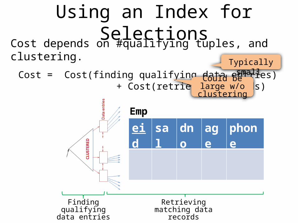
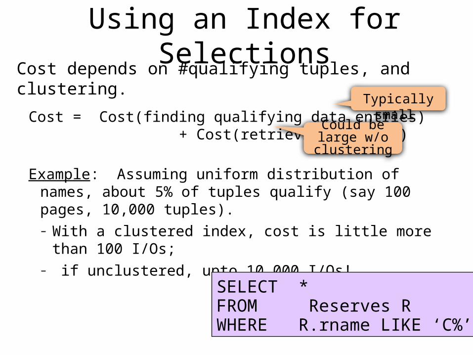
Using an Index for SelectionsCost depends on #qualifying tuples, and clustering.
Cost = Cost(finding qualifying data entries) + Cost(retrieving records)
Typically small
Could be large w/o clustering
Emp
eid sal dno age phone
Finding qualifying data entries
Retrieving matching data records
Using an Index for SelectionsCost depends on #qualifying tuples, and clustering.
Cost = Cost(finding qualifying data entries) + Cost(retrieving records)
Example: Assuming uniform distribution of names, about 5% of tuples qualify (say 100 pages, 10,000 tuples). – With a clustered index, cost is little more than 100
I/Os;– if unclustered, upto 10,000 I/Os!
SELECT *FROM Reserves RWHERE R.rname LIKE ‘C%’
Typically small
Could be large w/o clustering
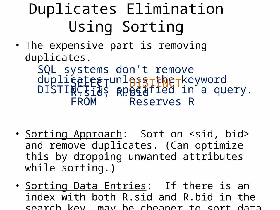
Duplicates Elimination Using Sorting
• The expensive part is removing duplicates.SQL systems don’t remove duplicates unless the keyword DISTINCT is specified in a query.
• Sorting Approach: Sort on <sid, bid> and remove duplicates. (Can optimize this by dropping unwanted attributes while sorting.)
• Sorting Data Entries: If there is an index with both R.sid and R.bid in the search key, may be cheaper to sort data entries!
SELECT DISTINCT R.sid, R.bidFROM Reserves R
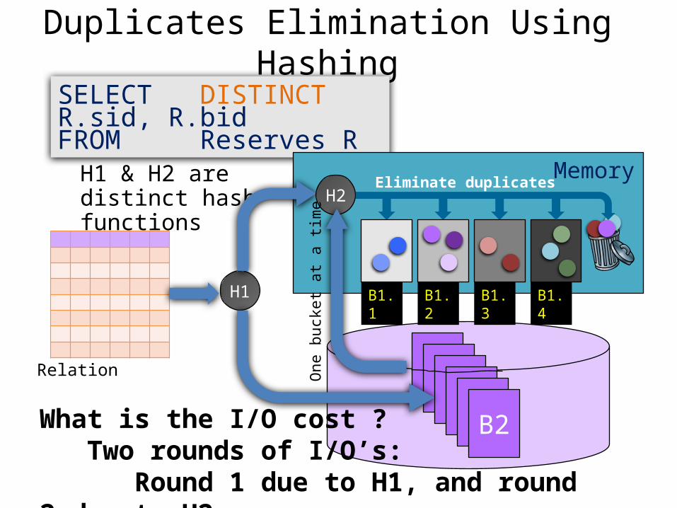
Duplicates Elimination Using HashingSELECT DISTINCT R.sid, R.bidFROM Reserves R
H1
Memory
B1B1B1B1B1B2What is the I/O cost ? Two rounds of I/O’s: Round 1 due to H1, and round 2 due to H2
H1 & H2 are distinct hash functions H2
B1.1 B1.2 B1.3 B1.4
Eliminate duplicates
One
buc
ket a
t a ti
me
Relation
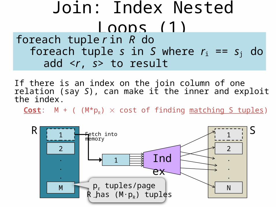
Join: Index Nested Loops (1)
If there is an index on the join column of one relation (say S), can make it the inner and exploit the index.
Cost: M + ( (M*pR) cost of finding matching S tuples)
foreach tuple r in R doforeach tuple s in S where ri == sj do
add <r, s> to result
1
2
M
.
.
.
R 1
2
N
.
.
.
S
1 Index
pr tuples/page→
Fetch intomemory
R has (M p∙ R) tuples
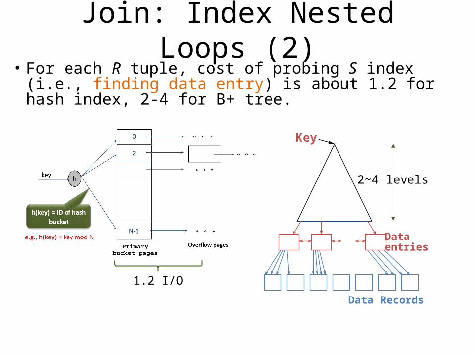
Join: Index Nested Loops (2)• For each R tuple, cost of probing S index (i.e., finding data
entry) is about 1.2 for hash index, 2-4 for B+ tree.
Dataentries
Data Records
Key
2~4 levels
1.2 I/O
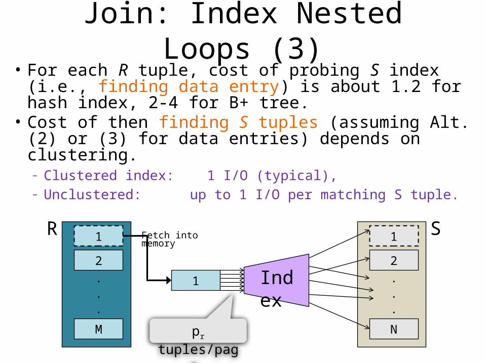
Join: Index Nested Loops (3)• For each R tuple, cost of probing S index (i.e., finding
data entry) is about 1.2 for hash index, 2-4 for B+ tree. • Cost of then finding S tuples (assuming Alt. (2) or (3)
for data entries) depends on clustering.– Clustered index: 1 I/O (typical), – Unclustered: up to 1 I/O per matching S tuple.
1
2
M
.
.
.
R
1 Index
1
2
N
.
.
.
S
pr tuples/page
Fetch intomemory
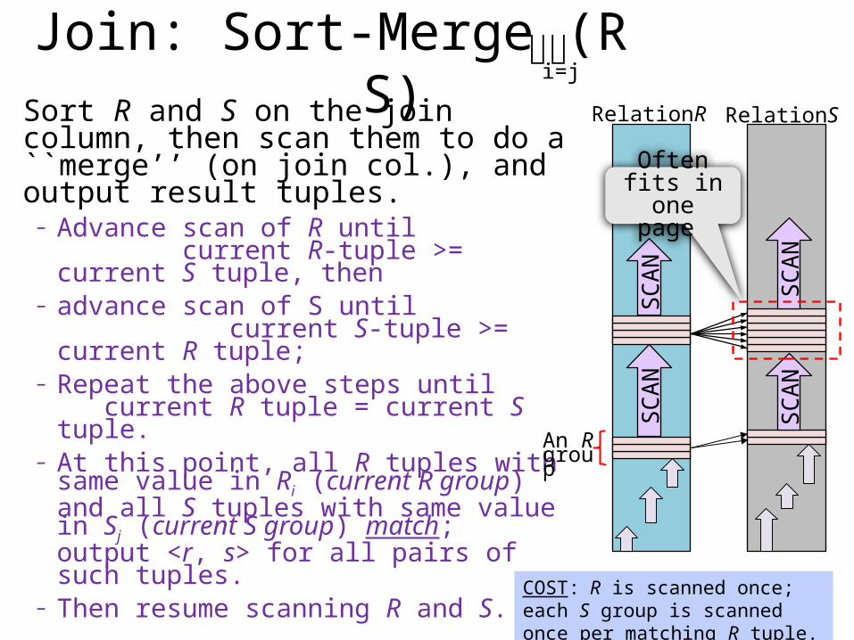
Join: Sort-Merge (R S)Sort R and S on the join column, then scan them to do a ``merge’’ (on join col.), and output result tuples.– Advance scan of R until
current R-tuple >= current S tuple, then – advance scan of S until
current S-tuple >= current R tuple; – Repeat the above steps until
current R tuple = current S tuple.– At this point, all R tuples with same
value in Ri (current R group) and all S tuples with same value in Sj (current S group) match; output <r, s> for all pairs of such tuples.
– Then resume scanning R and S.
i=j
SCAN
SCAN
SCAN SC
AN
RelationR RelationS
Often fits in one page
COST: R is scanned once; each S group is scanned once per matching R tuple.
An R group
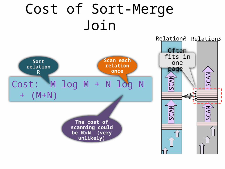
Cost of Sort-Merge Join
Cost: M log M + N log N + (M+N)
Scan each relation once
The cost of scanning could be MN (very
unlikely)
SCAN
SCAN
SCAN SC
AN
RelationR RelationS
Often fits in one page Sort relation
R
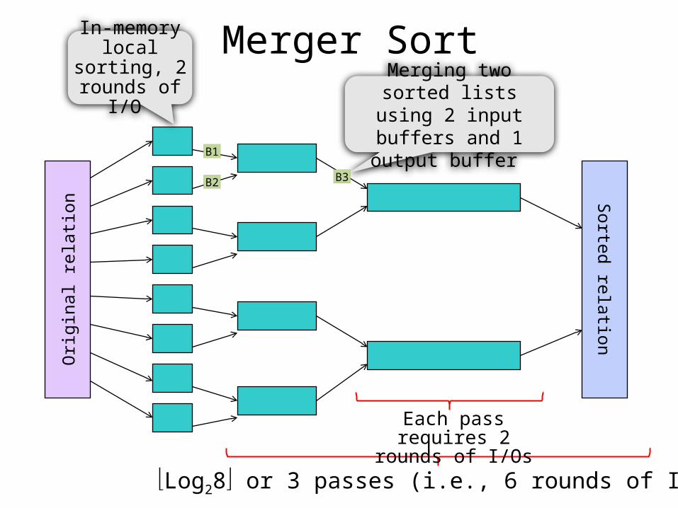
Merger SortO
rigin
al re
latio
nIn-memory
local sorting, 2 rounds of I/O Merging two sorted lists
using 2 input buffers and 1 output buffer
Log28 or 3 passes (i.e., 6 rounds of I/Os)
Each pass requires 2 rounds of I/Os
Sorted relation
B1
B2 B3

Highlights of System R Optimizer• Impact:
– Most widely used currently; works well for < 10 joins.
• Cost estimation: Approximate art at best.– Statistics, maintained in system catalogs, used to estimate
cost of operations and result sizes.– Considers combination of CPU and I/O costs.
• Plan Space: Too large, must be pruned.– Only the space of left-deep plans is considered.
• Left-deep plans allow output of each operator to be pipelined into the next operator without storing it in a temporary relation.
– Cartesian products avoided.O1
O2
O4
O3
R1 R2
R3
R4
R5
Left-deepplan
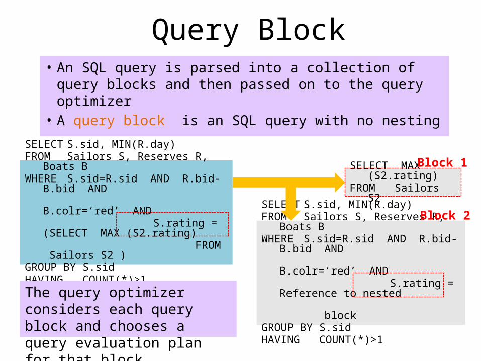
Query Block• An SQL query is parsed into a collection of query
blocks and then passed on to the query optimizer• A query block is an SQL query with no nesting
SELECT S.sid, MIN(R.day)FROM Sailors S, Reserves R, Boats BWHERE S.sid=R.sid AND R.bid-B.bid
AND B.colr=‘red’ AND S.rating = (SELECT MAX (S2.rating)
FROM Sailors S2 )GROUP BY S.sidHAVING COUNT(*)>1
SELECT S.sid, MIN(R.day)FROM Sailors S, Reserves R, Boats BWHERE S.sid=R.sid AND R.bid-B.bid
AND B.colr=‘red’ AND S.rating = Reference to nested blockGROUP BY S.sidHAVING COUNT(*)>1
SELECT MAX (S2.rating)FROM Sailors S2
The query optimizer considers each query block and chooses a query evaluation plan for that block.
Block 1
Block 2
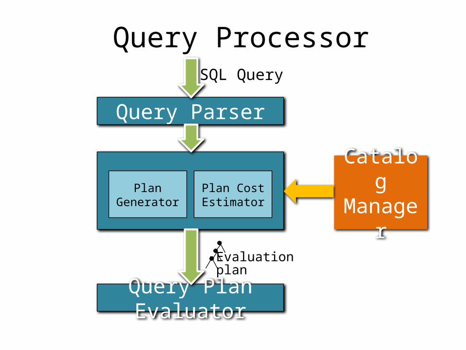
Query ProcessorSQL Query
Plan Generator
Plan CostEstimator
Evaluationplan
Query Parser
Catalog Manager
Query Plan Evaluator
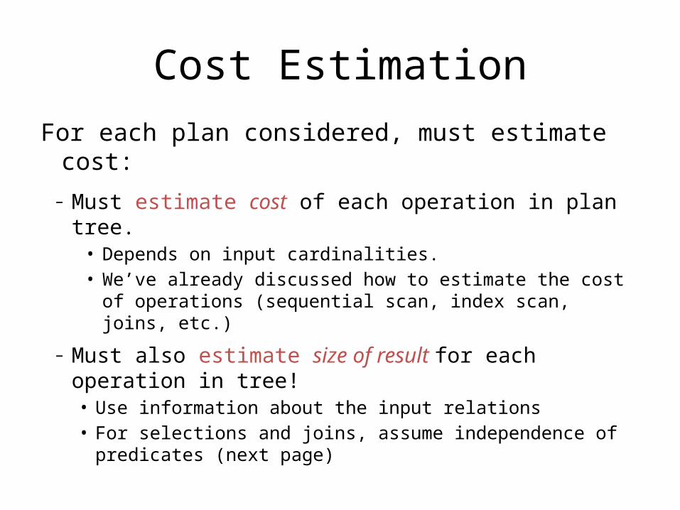
Cost Estimation
For each plan considered, must estimate cost:– Must estimate cost of each operation in plan tree.
• Depends on input cardinalities.• We’ve already discussed how to estimate the cost of
operations (sequential scan, index scan, joins, etc.)
– Must also estimate size of result for each operation in tree!• Use information about the input relations• For selections and joins, assume independence of
predicates (next page)
Size Estimation and Reduction Factors
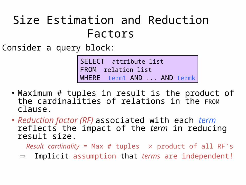
• Maximum # tuples in result is the product of the cardinalities of relations in the FROM clause.
• Reduction factor (RF) associated with each term reflects the impact of the term in reducing result size.
Result cardinality = Max # tuples product of all RF’s Implicit assumption that terms are independent!
SELECT attribute listFROM relation listWHERE term1 AND ... AND termk
Consider a query block:
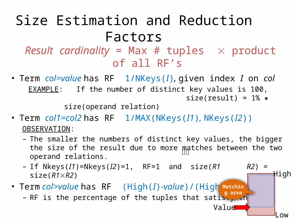
Size Estimation and Reduction Factors Result cardinality = Max # tuples product of all RF’s• Term col=value has RF 1/NKeys(I), given index I on col
EXAMPLE: If the number of distinct key values is 100, size(result) = 1% size(operand relation)
• Term col1=col2 has RF 1/MAX(NKeys(I1), NKeys(I2))OBSERVATION: – The smaller the numbers of distinct key values, the bigger the size of
the result due to more matches between the two operand relations. – If Nkeys(I1)=Nkeys(I2)=1, RF=1 and size(R1 R2) = size(R1R2)
• Term col>value has RF (High(I)-value)/(High(I)-Low(I))– RF is the percentage of the tuples that satisfy the term
High
LowValue
Matching area

Schema for ExamplesSailors (sid: integer, sname: string, rating: integer, age: real)Reserves (sid: integer, bid: integer, day: dates, rname: string)
.
.
.
Tuple is 50 bytes
80 tuples/page
500 pages
Sailors
.
.
.
Tuple is 40 bytes
100 tuples/page
1000 pages
Reserves
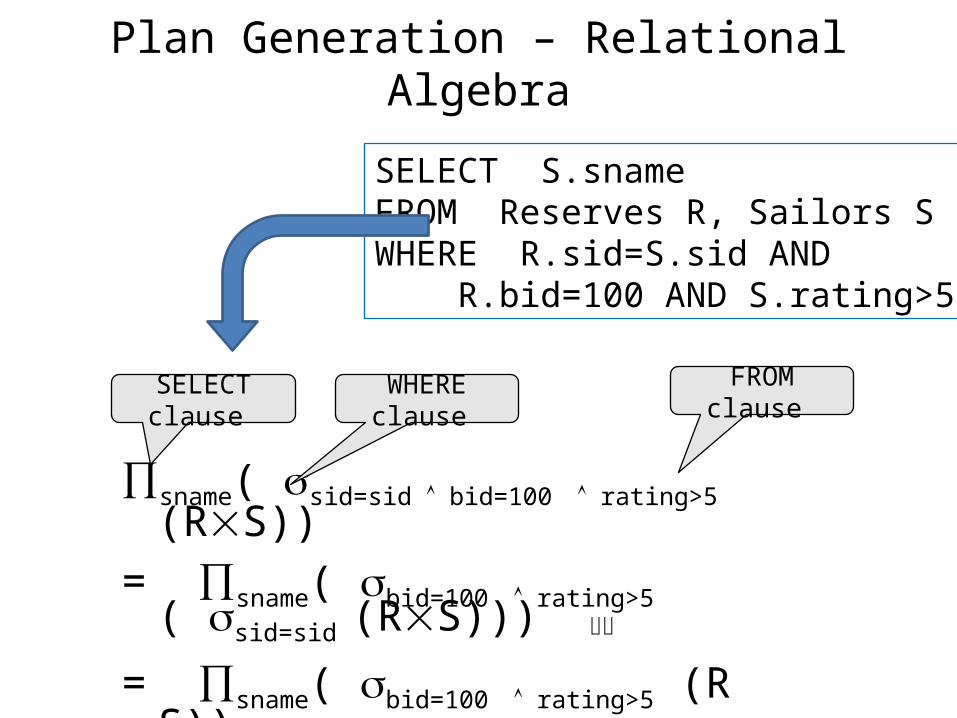
Plan Generation – Relational Algebra
SELECT S.snameFROM Reserves R, Sailors SWHERE R.sid=S.sid AND R.bid=100 AND S.rating>5
sname( sid=sid bid=100 rating>5 (RS))
= sname( bid=100 rating>5 ( sid=sid (RS)))
= sname( bid=100 rating>5 (R S))
FROM clause WHERE clause SELECT clause
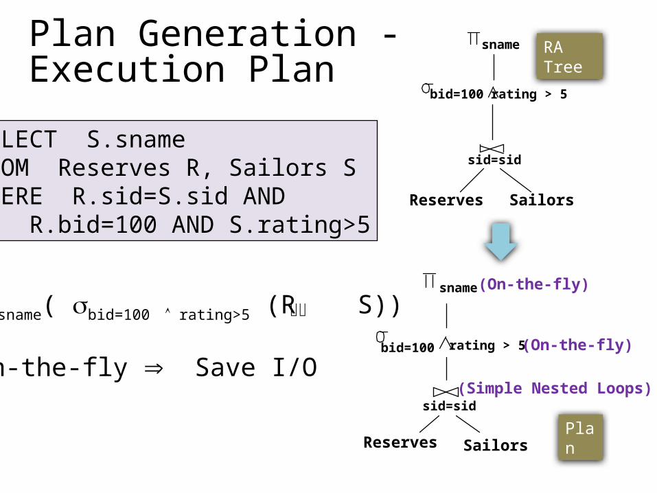
Plan Generation - Execution Plan
SELECT S.snameFROM Reserves R, Sailors SWHERE R.sid=S.sid AND R.bid=100 AND S.rating>5
Reserves Sailors
sid=sid
bid=100 rating > 5
sname RA Tree
Reserves Sailors
sid=sid
bid=100 rating > 5
sname
(Simple Nested Loops)
(On-the-fly)
(On-the-fly)
Plan
sname( bid=100 rating>5 (R S))
On-the-fly Save I/O
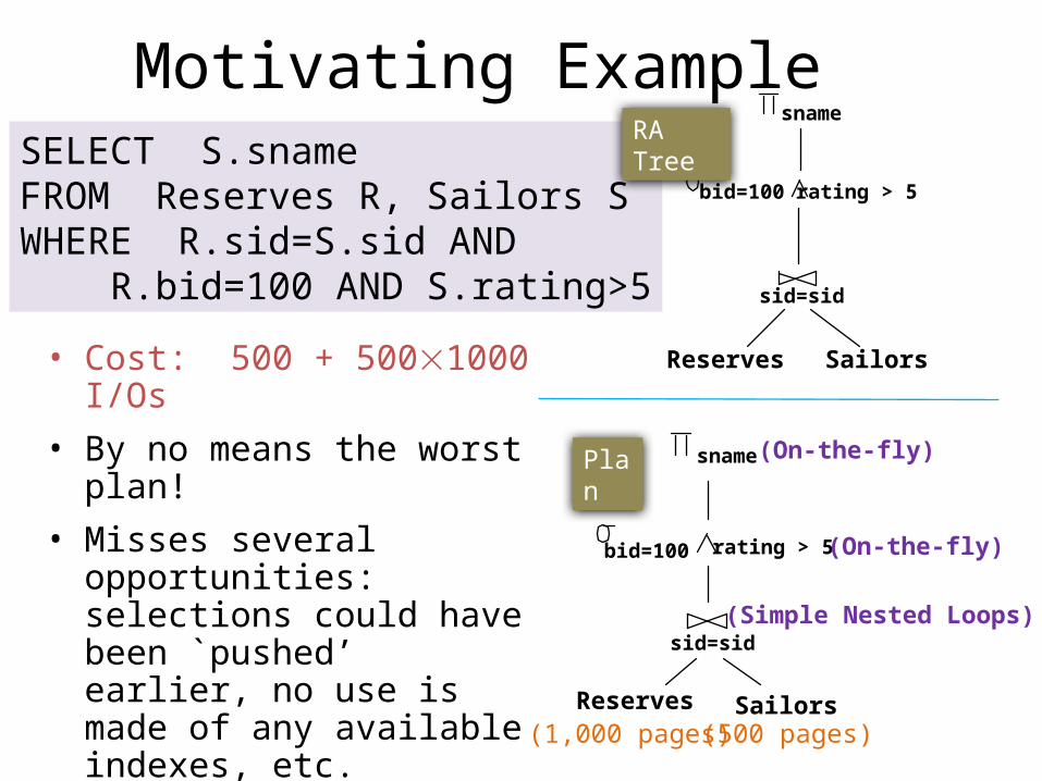
Motivating Example
• Cost: 500 + 5001000 I/Os• By no means the worst plan! • Misses several opportunities:
selections could have been `pushed’ earlier, no use is made of any available indexes, etc.
• Goal of optimization: To find more efficient plans that compute the same answer.
SELECT S.snameFROM Reserves R, Sailors SWHERE R.sid=S.sid AND R.bid=100 AND S.rating>5
Reserves Sailors
sid=sid
bid=100 rating > 5
snameRA Tree
Reserves Sailors
sid=sid
bid=100 rating > 5
sname
(Simple Nested Loops)
(On-the-fly)
(On-the-fly)Plan
(1,000 pages) (500 pages)
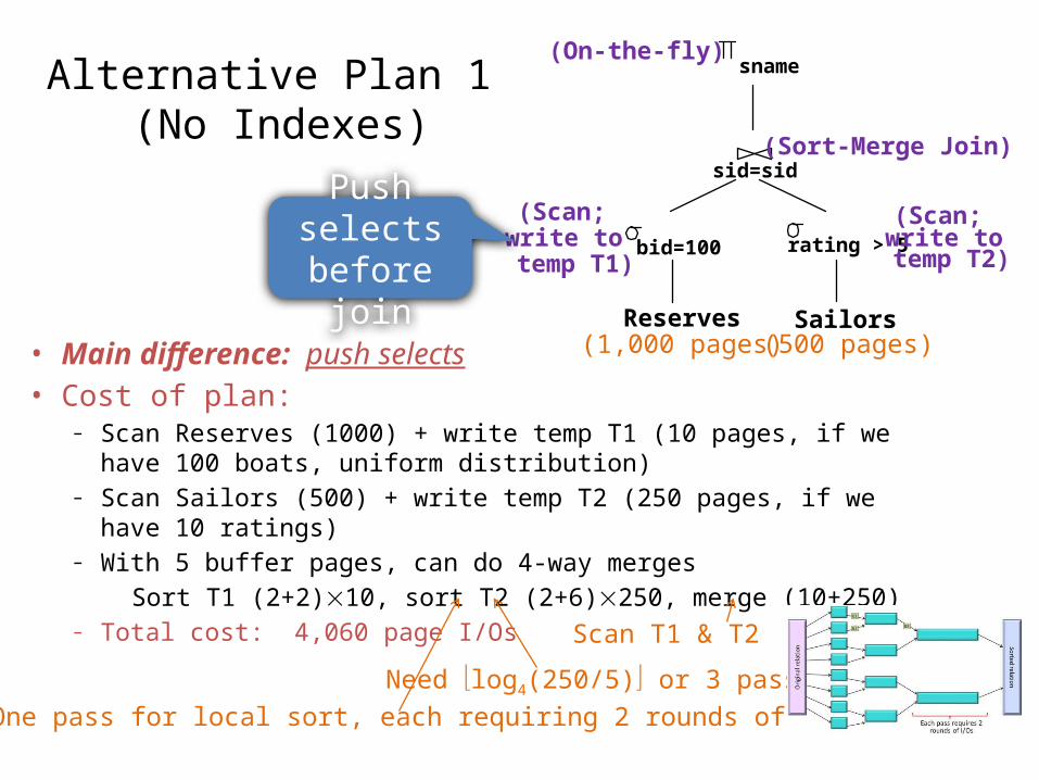
Alternative Plan 1 (No Indexes)
• Main difference: push selects• Cost of plan:
– Scan Reserves (1000) + write temp T1 (10 pages, if we have 100 boats, uniform distribution)
– Scan Sailors (500) + write temp T2 (250 pages, if we have 10 ratings)– With 5 buffer pages, can do 4-way merges
Sort T1 (2+2)10, sort T2 (2+6)250, merge (10+250)– Total cost: 4,060 page I/Os
Reserves Sailors
sid=sid
bid=100
sname(On-the-fly)
rating > 5
(Scan;write to temp T1)
(Scan;write totemp T2)
(Sort-Merge Join)
Push selects before join
(1,000 pages) (500 pages)
Need log4(250/5) or 3 passesOne pass for local sort, each requiring 2 rounds of I/Os
Scan T1 & T2
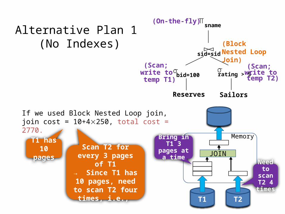
Alternative Plan 1 (No Indexes)
If we used Block Nested Loop join, join cost = 10+4250, total cost = 2770.
Reserves Sailors
sid=sid
bid=100
sname(On-the-fly)
rating > 5
(Scan;write to temp T1)
(Scan;write totemp T2)
(Block Nested Loop Join)
Scan T2 for every 3 pages of T1
→ Since T1 has 10 pages, need to scan T2
four times, i.e.,
T1 has 10 pages
T1 T2
JOIN
MemoryBring in T1 3 pages at
a time
Need to scan T2 4 times
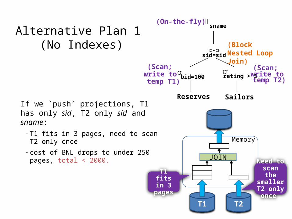
Alternative Plan 1 (No Indexes)
Reserves Sailors
sid=sid
bid=100
sname(On-the-fly)
rating > 5
(Scan;write to temp T1)
(Scan;write totemp T2)
(Block Nested Loop Join)
T1 T2
JOIN
Memory
T1 fits in 3 pages
Need to scan the
smaller T2 only once
If we `push’ projections, T1 has only sid, T2 only sid and sname:– T1 fits in 3 pages, need to scan T2
only once– cost of BNL drops to under 250
pages, total < 2000.
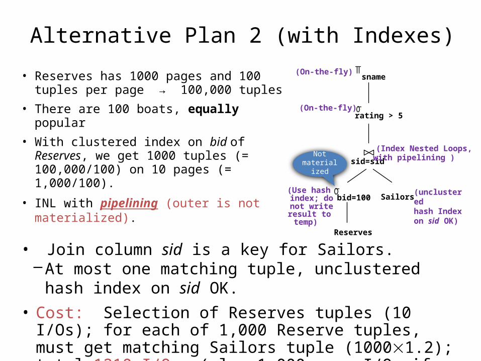
Alternative Plan 2 (with Indexes)• Reserves has 1000 pages and 100 tuples
per page → 100,000 tuples• There are 100 boats, equally popular• With clustered index on bid of Reserves,
we get 1000 tuples (= 100,000/100) on 10 pages (= 1,000/100).
• INL with pipelining (outer is not materialized).
Reserves
Sailors
sid=sid
bid=100
sname(On-the-fly)
rating > 5
(Use hashindex; donot writeresult to temp)
(Index Nested Loops,with pipelining )
(On-the-fly)
• Join column sid is a key for Sailors.– At most one matching tuple, unclustered hash index on sid OK.
• Cost: Selection of Reserves tuples (10 I/Os); for each of 1,000 Reserve tuples, must get matching Sailors tuple (10001.2); total 1210 I/Os (plus 1,000 more I/Os if Sailors stored as alternative 2)
(unclusteredhash Index on sid OK)
Not materialized
Alternative Plan 2 (continued …)
Reserves
Sailors
sid=sid
bid=100
sname(On-the-fly)
rating > 5
(Use hash index; do not write result to temp)
(Index Nested Loops,with pipelining )
(On-the-fly)
(unclusteredIndex on sid OK)
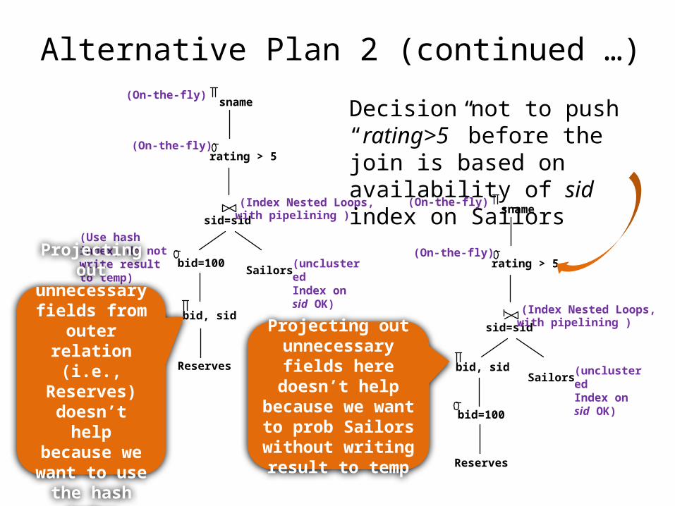
Decision not to push “rating>5” before the join is based on availability of sid index on Sailors
bid, sidProjecting out unnecessary
fields from outer relation (i.e.,
Reserves) doesn’t help because we
want to use the hash index Reserves
Sailors
sid=sid
bid=100
sname(On-the-fly)
rating > 5
(Index Nested Loops,with pipelining )
(On-the-fly)
(unclusteredIndex on sid OK)
bid, sid
Projecting out unnecessary fields here doesn’t help
because we want to prob Sailors without
writing result to temp
Summary• There are several alternative evaluation algorithms for each
relational operator.• A query is evaluated by converting it to a tree of operators and
evaluating the operators in the tree.• Must understand query optimization in order to fully
understand the performance impact of a given database design (relations, indexes) on a workload (set of queries).
• Two parts to optimizing a query:– Consider a set of alternative plans.
• Must prune search space; typically, left-deep plans only.
– Must estimate cost of each plan that is considered.• Must estimate size of result and cost for each plan node.• Key issues: Statistics, indexes, operator implementations.