Computational SemanticsDay 4: Dominance Graphs, Round Two

Aljoscha BurchardtAlexander Koller

Stephan Walter

ESSLLI 2004, Nancy

Overview

u Semantics construction for dominance graphs

u Implementation in our Prolog framework

u Solving dominance graphs

u Implementing the graph solver

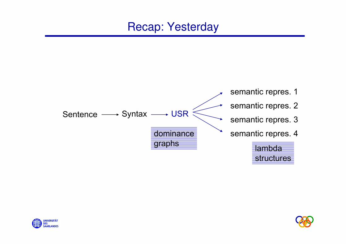
Recap: Yesterday

Sentence

semantic repres. 1semantic repres. 2semantic repres. 3semantic repres. 4

Syntax USRdominancegraphs lambda

structures

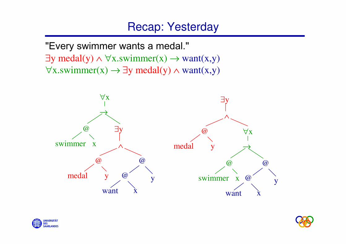
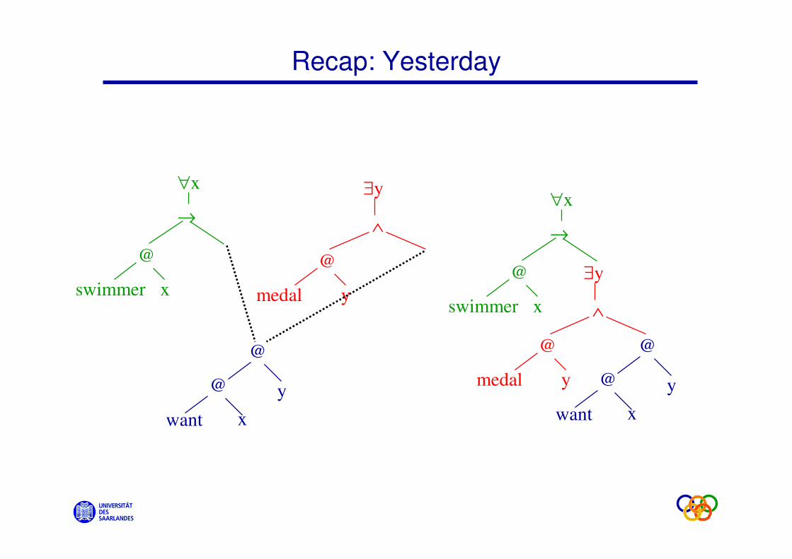
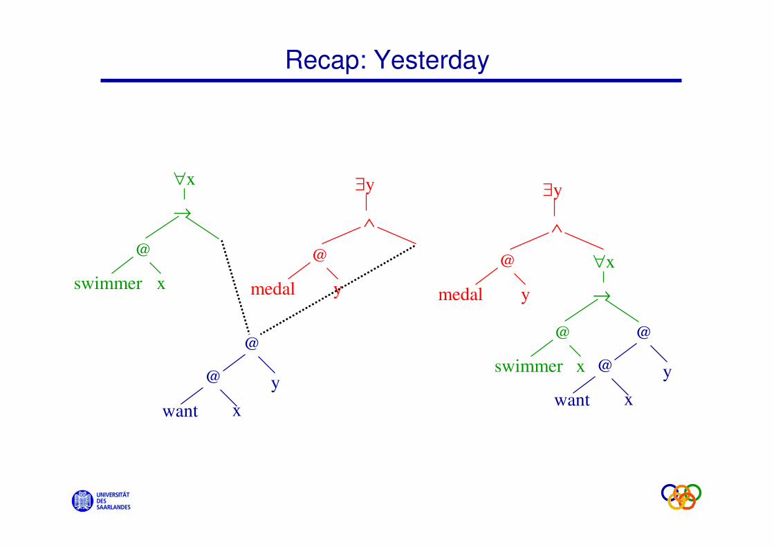
Recap: Yesterday

"Every swimmer wants a medal."∃y medal(y) ∧ ∀x.swimmer(x) → want(x,y)

∀x.swimmer(x) → ∃y medal(y) ∧ want(x,y)

∀x

swimmer

→

x

@ ∃y

medal y

∧

@

want x

y

@

@

∀x

swimmer

→

x

@

∃y

medal y

∧

@

want x

y

@

@

Recap: Yesterday

∀x

swimmer

→

x

@ ∃y

medal y

∧

@

want x

y

@

@

∀x

swimmer

→

x

@

∃y

medal y

∧

@

want x

y

@

@

Recap: Yesterday

∀x

swimmer

→

x

@

∃y

medal y

∧

@

want x

y

@

@

∀x

swimmer

→

x

@

∃y

medal y

∧

@

want x

y

@

@

Semantics Construction

u First remaining question:

– How do we construct a dominance graph

from a syntactic analysis?

u We use Tuesday's modular syntax-semantics

framework.

u Replace semantic macros and combine rules

by new ones.

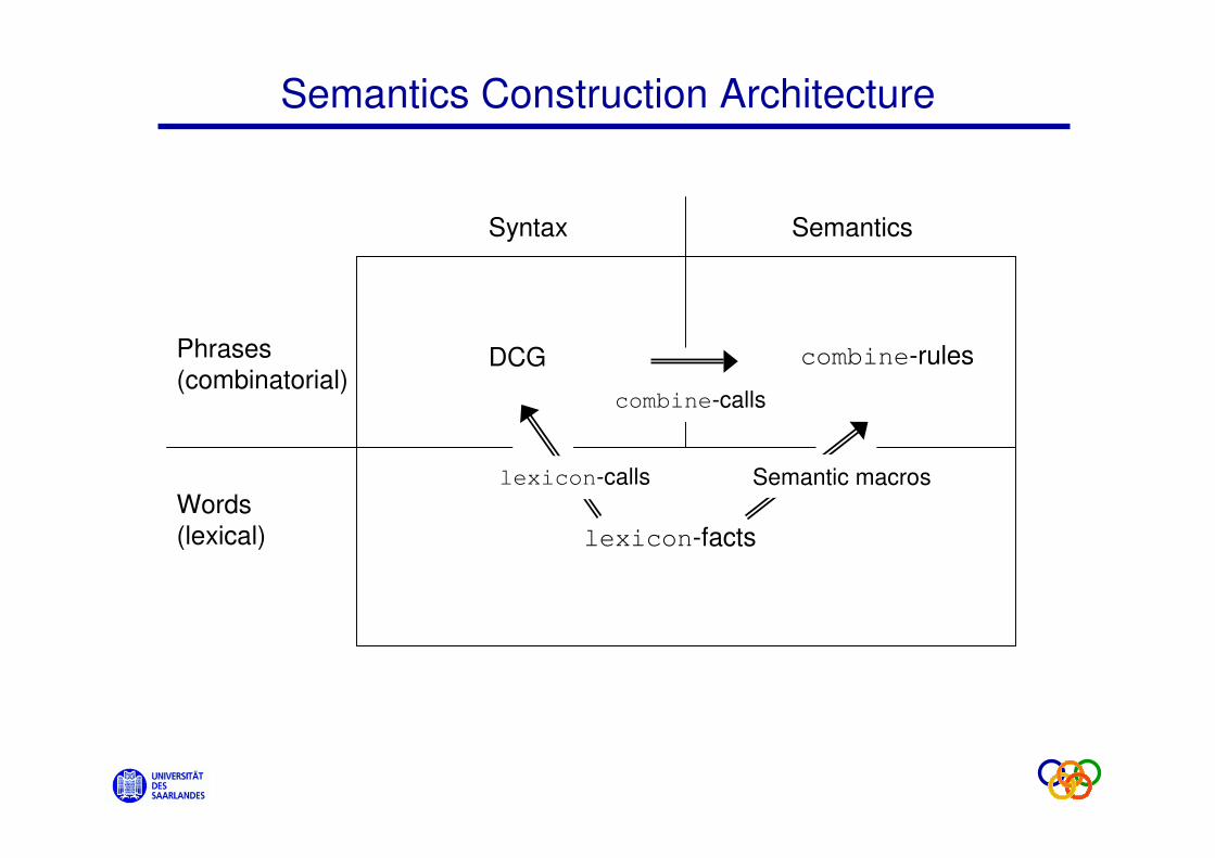
Semantics Construction Architecture

Words

(lexical)

Phrases

(combinatorial)

Syntax Semantics

DCG combine-rules

lexicon-facts

lexicon-calls Semantic macros

combine-calls

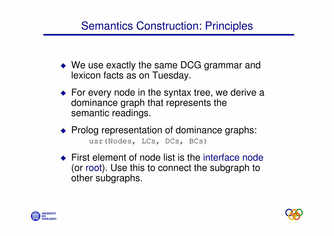
Semantics Construction: Principles

u We use exactly the same DCG grammar and lexicon facts as on Tuesday.

u For every node in the syntax tree, we derive a dominance graph that represents the semantic readings.

u Prolog representation of dominance graphs:usr(Nodes, LCs, DCs, BCs)

u First element of node list is the interface node (or root). Use this to connect the subgraph to other subgraphs.

A Simple Example

PN TV PN

Ian beats Michael

NP NP

VP

S

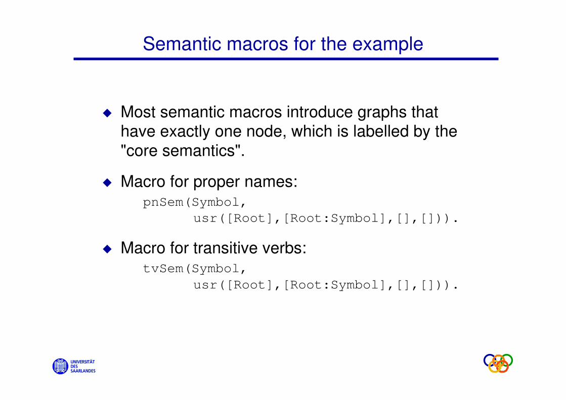
Semantic macros for the example

u Most semantic macros introduce graphs that have exactly one node, which is labelled by the

"core semantics".

u Macro for proper names:pnSem(Symbol,

usr([Root],[Root:Symbol],[],[])).

u Macro for transitive verbs:tvSem(Symbol,

usr([Root],[Root:Symbol],[],[])).

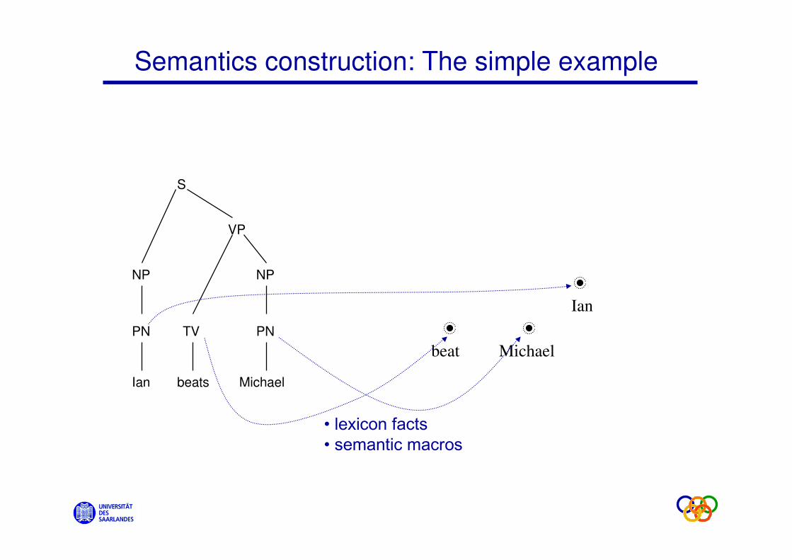
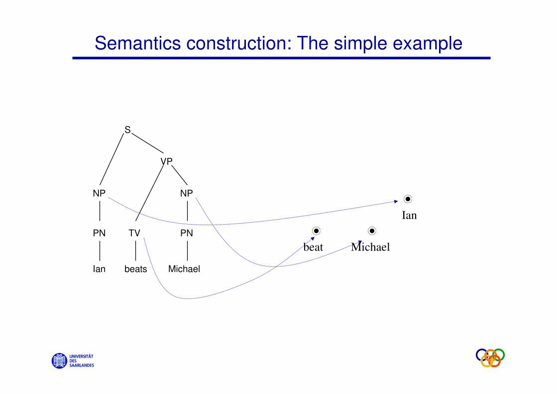
Semantics construction: The simple example

PN TV PN

Ian beats Michael

NP NP

VP

S

beat Michael

Ian

• lexicon facts• semantic macros

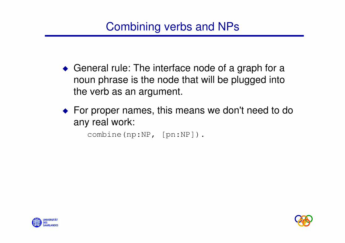
Combining verbs and NPs

u General rule: The interface node of a graph for a noun phrase is the node that will be plugged into

the verb as an argument.

u For proper names, this means we don't need to do

any real work:combine(np:NP, [pn:NP]).

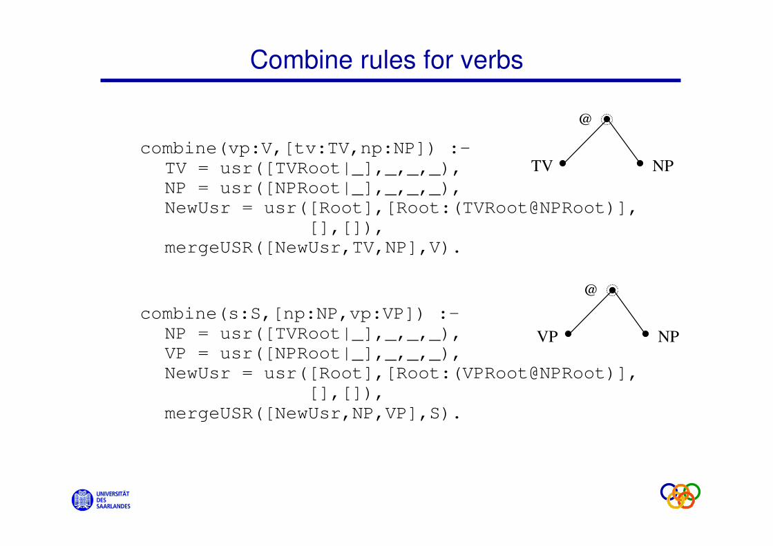
Combine rules for verbs

combine(vp:V,[tv:TV,np:NP]) :-

TV = usr([TVRoot|_],_,_,_),

NP = usr([NPRoot|_],_,_,_),

NewUsr = usr([Root],[Root:(TVRoot@NPRoot)],

[],[]),

mergeUSR([NewUsr,TV,NP],V).

combine(s:S,[np:NP,vp:VP]) :-

NP = usr([TVRoot|_],_,_,_),

VP = usr([NPRoot|_],_,_,_),

NewUsr = usr([Root],[Root:(VPRoot@NPRoot)],

[],[]),

mergeUSR([NewUsr,NP,VP],S).

@

TV NP

@

VP NP

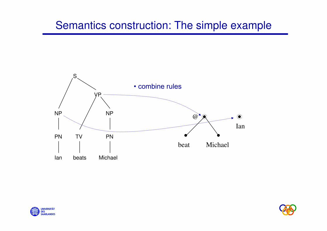
Semantics construction: The simple example

PN TV PN

Ian beats Michael

NP NP

VP

S

beat Michael

Ian

Semantics construction: The simple example

PN TV PN

Ian beats Michael

NP NP

VP

S

beat Michael

Ian

@

• combine rules

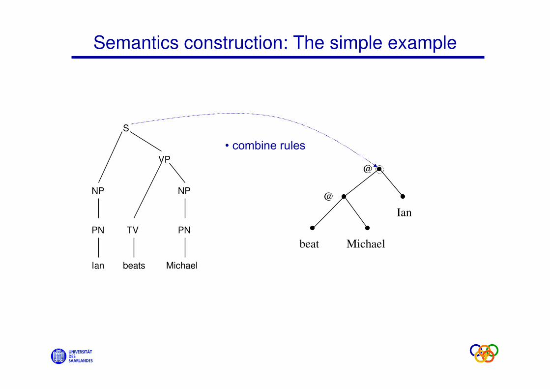
Semantics construction: The simple example

PN TV PN

Ian beats Michael

NP NP

VP

S

beat Michael

Ian

@

@

• combine rules

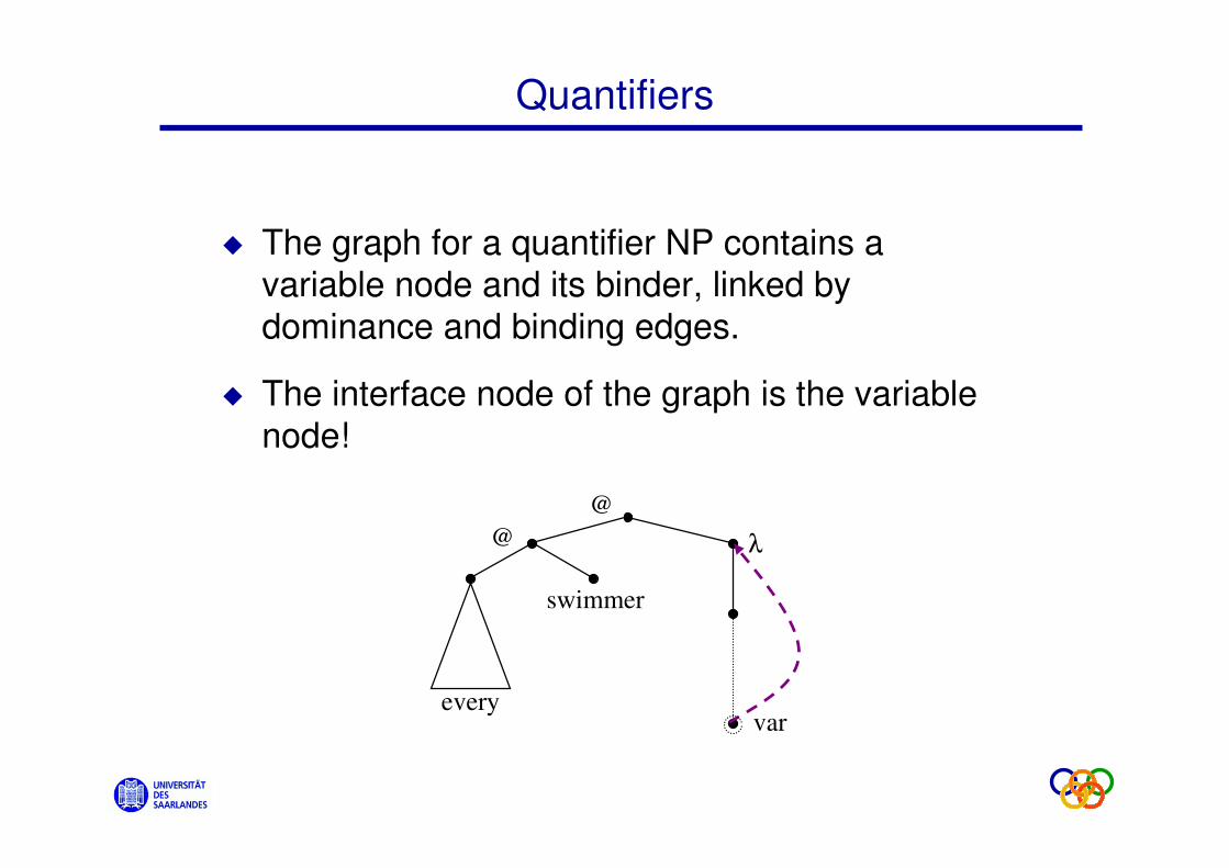
Quantifiers

u The graph for a quantifier NP contains a variable node and its binder, linked by

dominance and binding edges.

u The interface node of the graph is the variable

node!

every

swimmer

λ

var

@

@

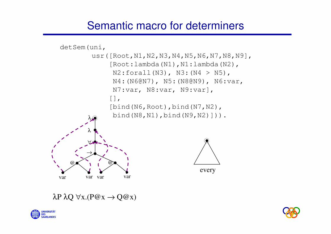
Semantic macro for determiners

detSem(uni,

usr([Root,N1,N2,N3,N4,N5,N6,N7,N8,N9],

[Root:lambda(N1),N1:lambda(N2),

N2:forall(N3), N3:(N4 > N5),

N4:(N6@N7), N5:(N8@N9), N6:var,

N7:var, N8:var, N9:var],

[],

[bind(N6,Root),bind(N7,N2),

bind(N8,N1),bind(N9,N2)])).

@

var var

@

var var

λ

λ

∀

→

every

λP λQ ∀x.(P@x → Q@x)

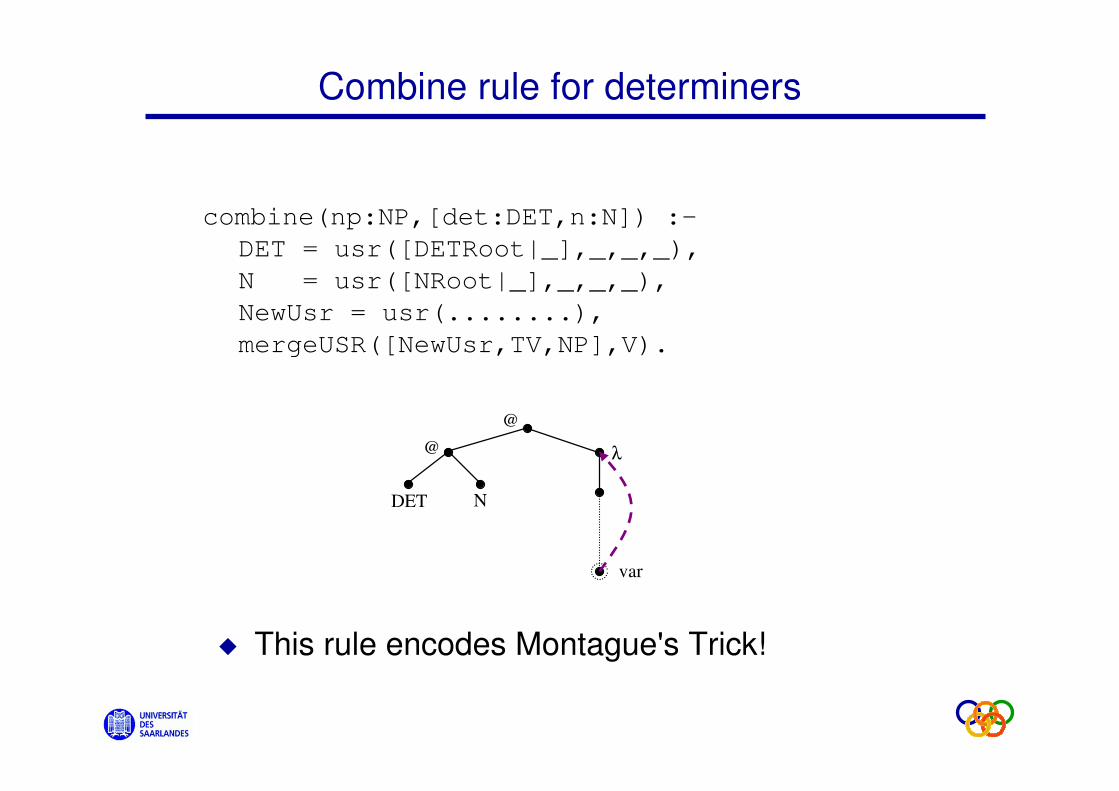
Combine rule for determiners

combine(np:NP,[det:DET,n:N]) :-

DET = usr([DETRoot|_],_,_,_),

N = usr([NRoot|_],_,_,_),

NewUsr = usr(........),

mergeUSR([NewUsr,TV,NP],V).

@

@

DET N

λ

var

u This rule encodes Montague's Trick!

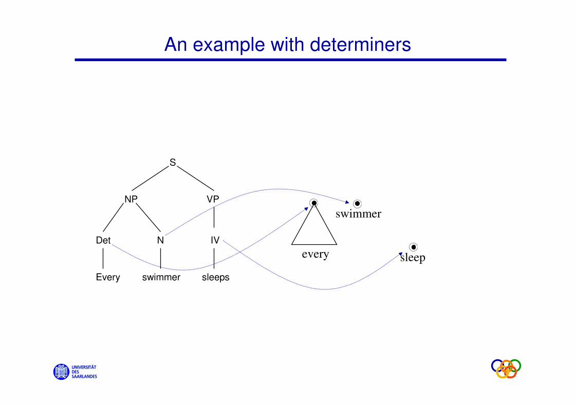
An example with determiners

Det N IV

Every sleepsswimmer

NP VP

S

every

swimmer

sleep

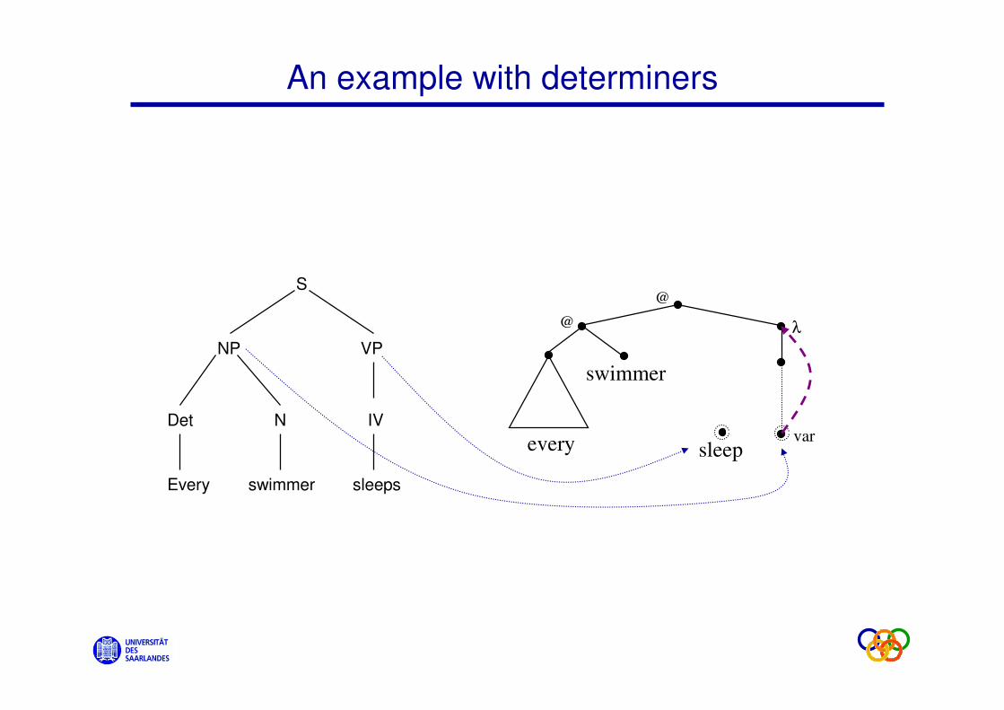
An example with determiners

Det N IV

Every sleepsswimmer

NP VP

S

every

swimmer

sleep

@

@

λ

var

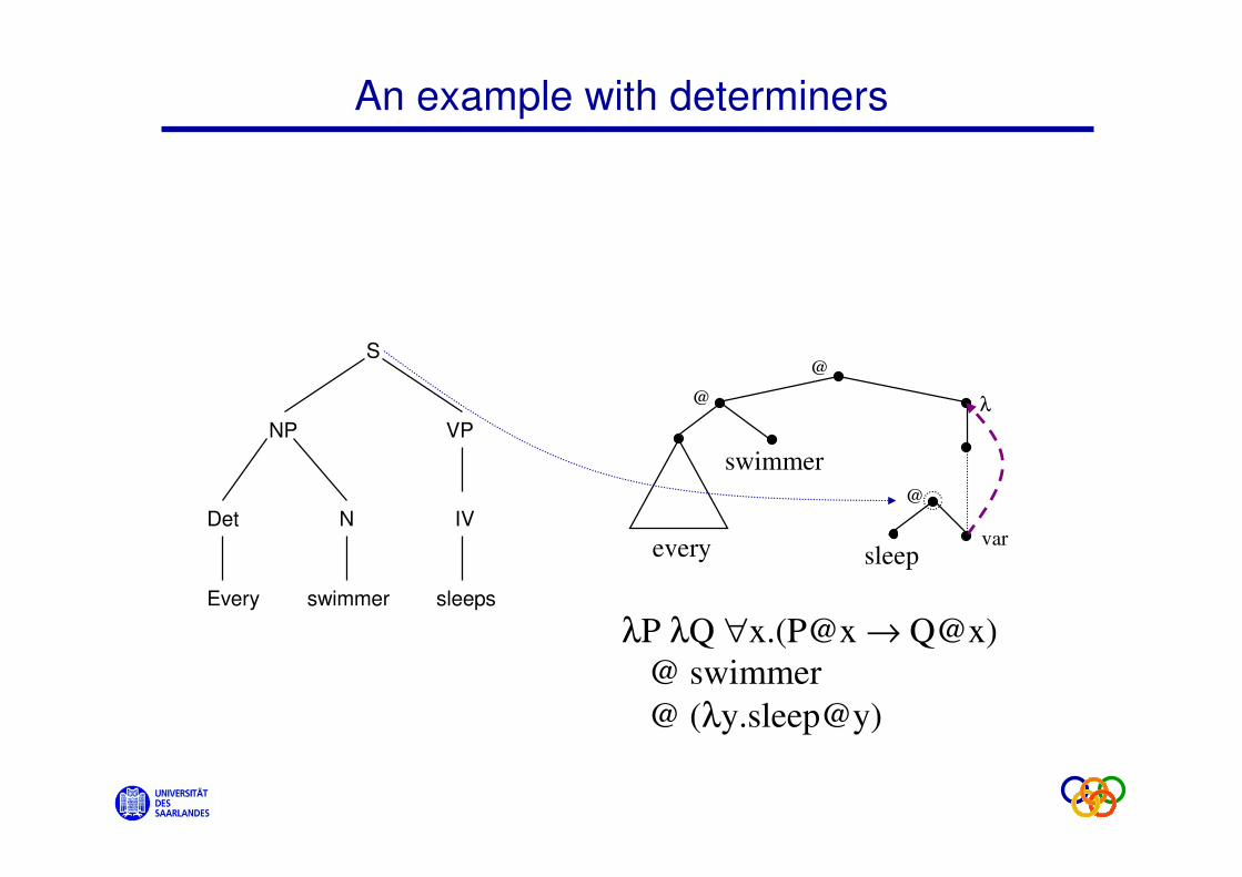
An example with determiners

Det N IV

Every sleepsswimmer

NP VP

S

every

swimmer

sleep

@

@

λ

@

var

λP λQ ∀x.(P@x → Q@x)

@ swimmer

@ (λy.sleep@y)

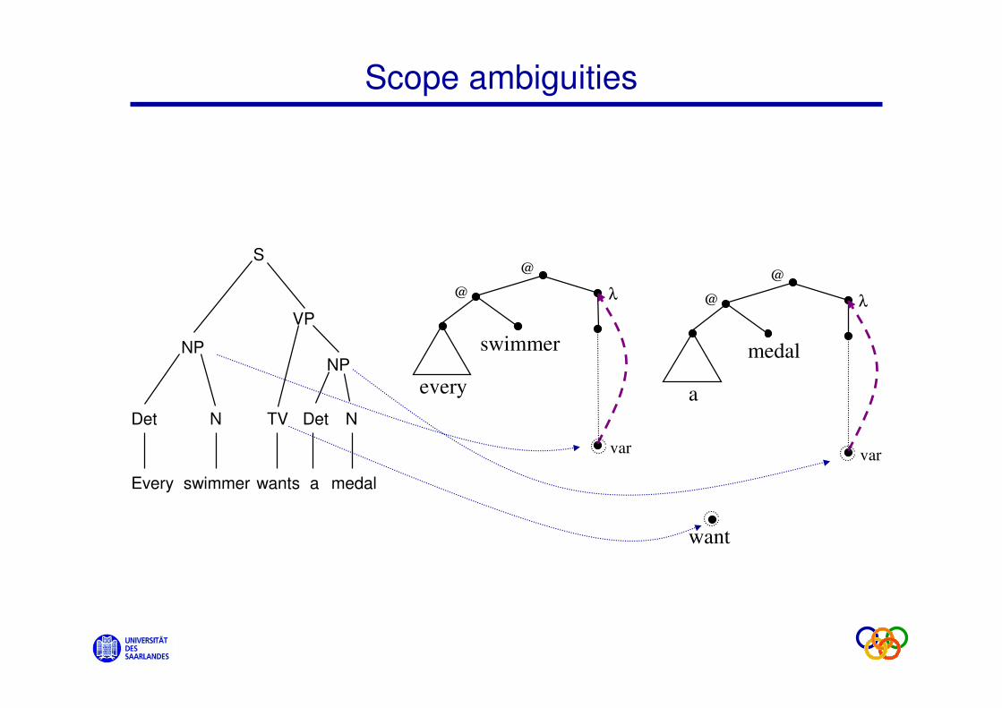
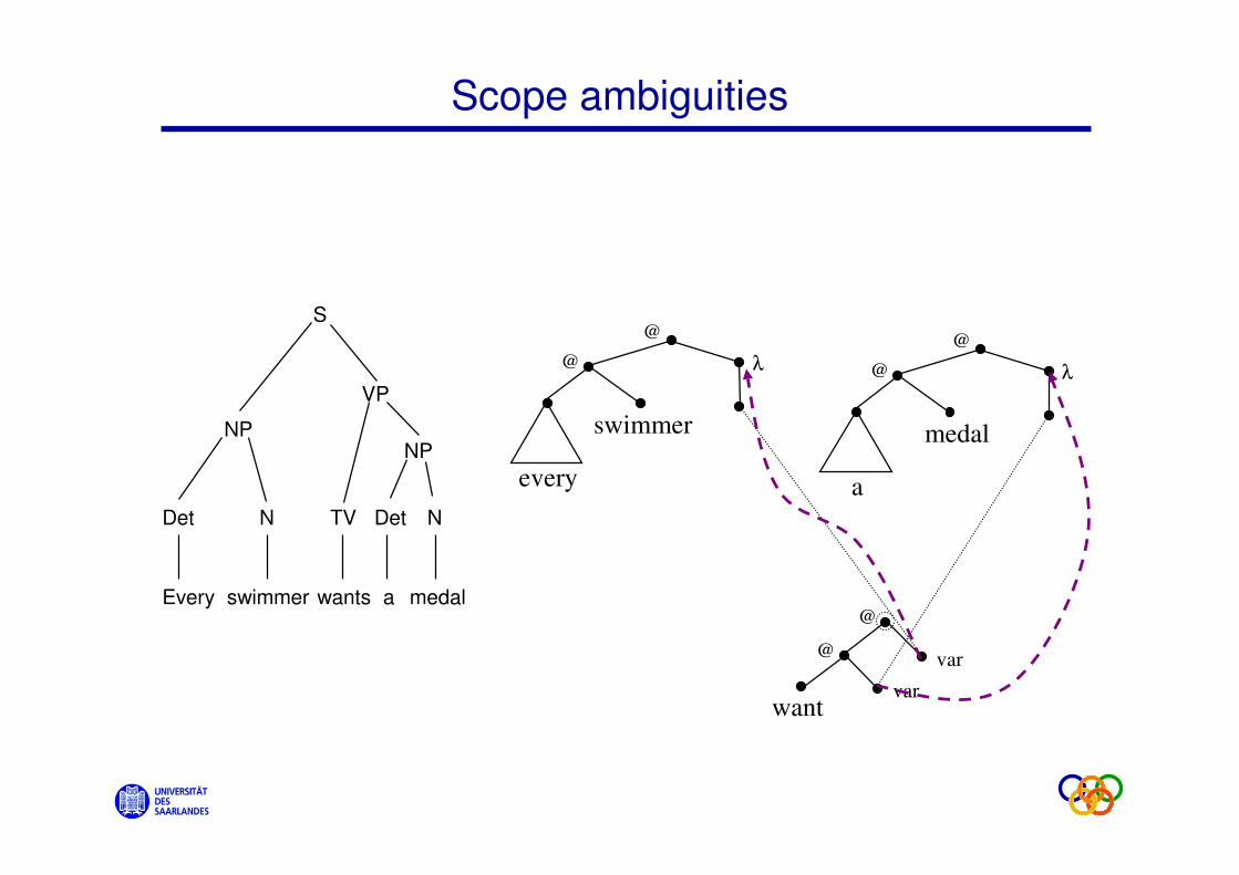
Scope ambiguities

Det N TV

Every wantsswimmer

NP

VP

S

Det

a

N

medal

NP

every

swimmer

@

@

λ

var

a

medal

@

@

λ

var

want

Scope ambiguities

Det N TV

Every wantsswimmer

NP

VP

S

Det

a

N

medal

NP

every

swimmer

@

@

λ

var

a

medal

@

@

λ

varwant

@

Scope ambiguities

Det N TV

Every wantsswimmer

NP

VP

S

Det

a

N

medal

NP

every

swimmer

@

@

λ

var

a

medal

@

@

λ

varwant

@

@

Semantics construction: Summary

u By plugging new rules into yesterday's syntax-semantics framework, we can compute

dominance graphs for English sentences.

u Changed semantic macros to give us

dominance graphs for lexicon entries.

u Combine rules plug subgraphs together by

connecting their interface nodes.

u Always apply verb semantics to interface

variable of an argument NP.

Underspecification in semantics construction

u Combine rule of determiners encodes Montague's Trick.

u Variable and binder are introduced together: No capturing necessary!

u Need fewer lambdas because we can now talk about positions in formulas explicitly.

u All large-scale grammars with semantics use some form of underspecification.

Solving Dominance Graphs

u Now we know

– how to model scope ambiguities with

dominance graphs

– how to represent dominance graphs in

Prolog

– how to compute dominance graphs for

English sentences.

u What's still missing: How to compute the trees

(= formulas) that a graph represents?

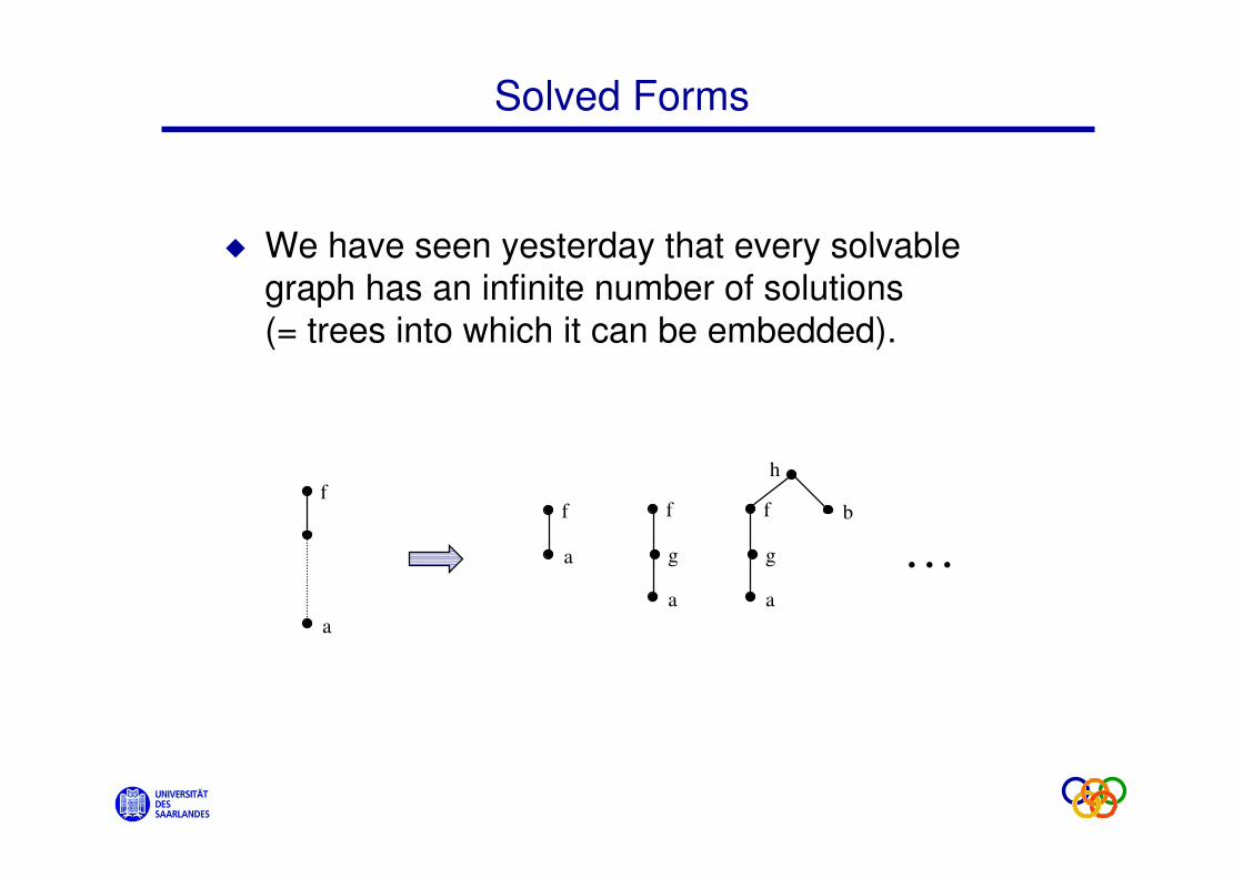
Solved Forms

u We have seen yesterday that every solvable graph has an infinite number of solutions

(= trees into which it can be embedded).

f

a

f

a

f

a

g

f

a

g

h

b

. . .

Solved Forms

u Thus, we aim at enumerating all solved formsof a dominance graph and not all solutions.

u A dominance graph in solved form is a graph whose tree and dominance edges are a

forest.

u A graph G' is a solved form of G iff G' is in

solved form and if there is a path from u to v in G (over tree and dominance edges), there is

also a path from u to v in G'.

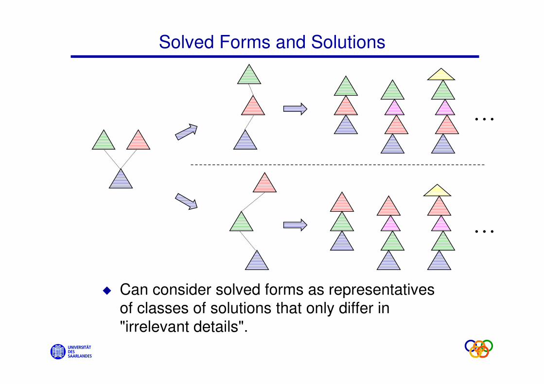
Solved Forms and Solutions

u Can consider solved forms as representatives of classes of solutions that only differ in

"irrelevant details".

. . .

. . .

Solving Dominance Graphs

u Solver algorithm applies three graph simplification rules and then calls itself

recursively:

– Choice

– Parent Normalisation

– Redundancy Elimination

u Detect unsolvability: Test for cycles.

u Prolog implementation.

The Choice Rule

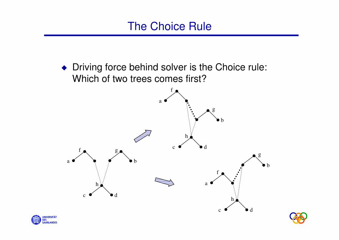
u Driving force behind solver is the Choice rule: Which of two trees comes first?

a

f

b

g

d

h

c

a

f

b

g

d

h

c

a

f

b

g

d

h

c

The Choice Rule

u Every application of Choice arranges the dominance parents of one node.

u Eventually, the dominance parents of all nodes will be arranged.

u Choice rule is sound: Every tree that satisfies original graph also satisfies one of the two

possible results of the Choice application.

Cleaning Up I: Parent Normalisation

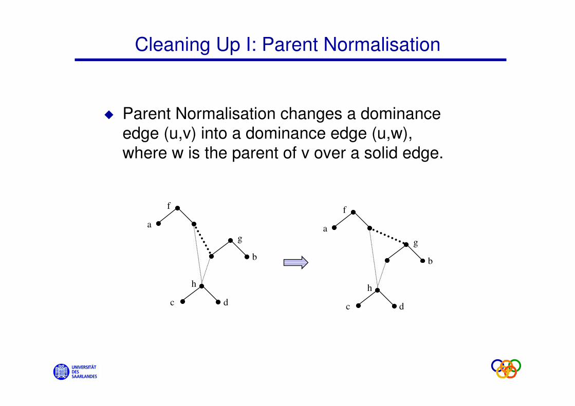
u Parent Normalisation changes a dominance edge (u,v) into a dominance edge (u,w),

where w is the parent of v over a solid edge.

a

f

b

g

d

h

c

a

f

b

g

d

h

c

Cleaning Up II: Redundancy Elimination

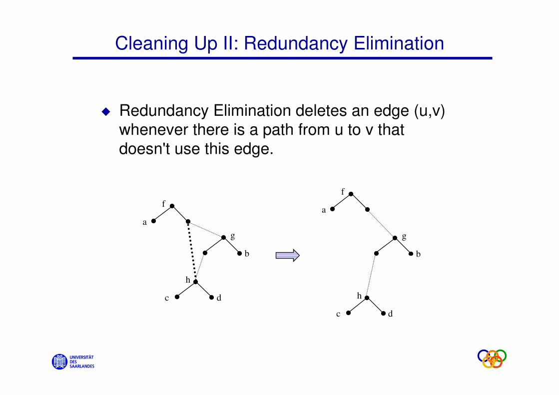
u Redundancy Elimination deletes an edge (u,v) whenever there is a path from u to v that

doesn't use this edge.

a

f

b

g

d

h

c

a

f

b

g

d

h

c

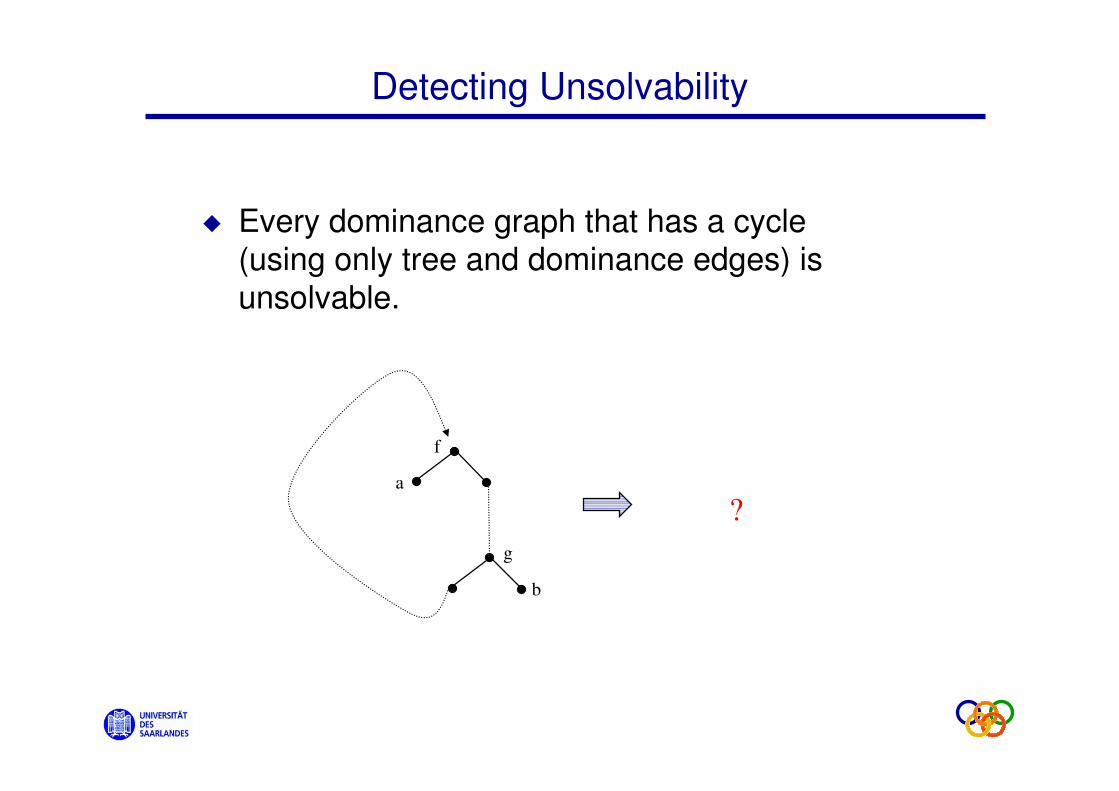
Detecting Unsolvability

u Every dominance graph that has a cycle (using only tree and dominance edges) is

unsolvable.

a

f

b

g

?

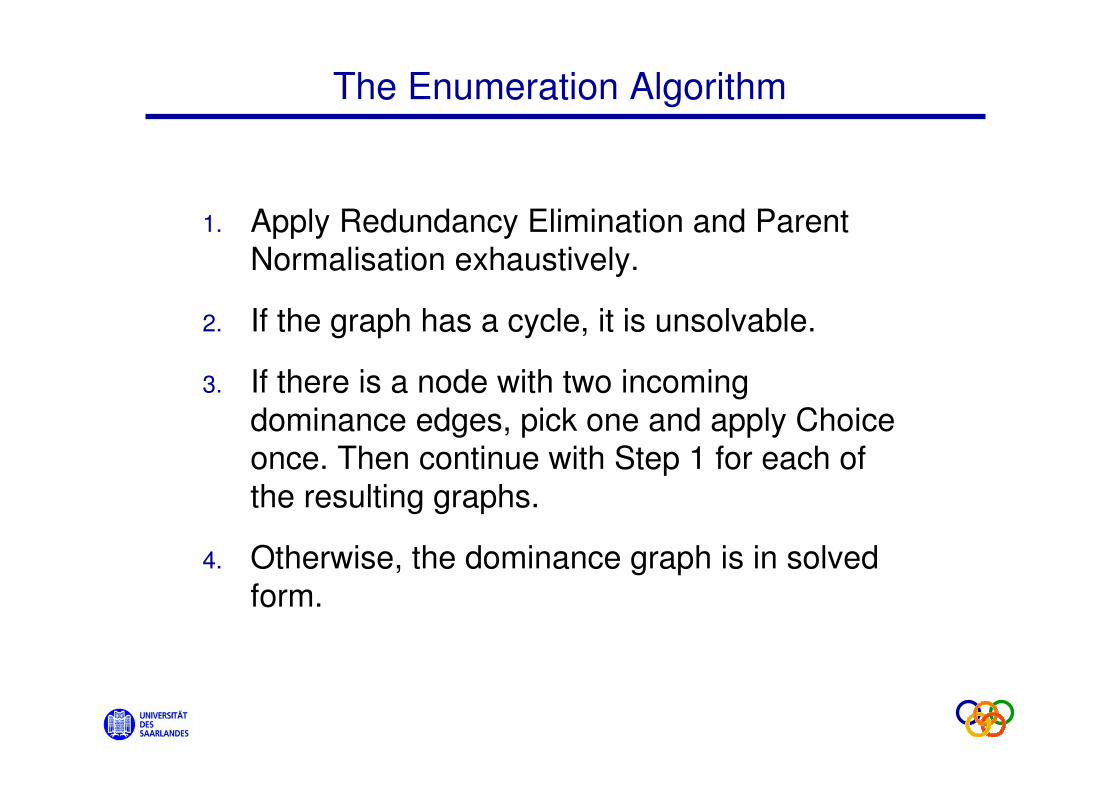
The Enumeration Algorithm

1. Apply Redundancy Elimination and Parent Normalisation exhaustively.

2. If the graph has a cycle, it is unsolvable.

3. If there is a node with two incoming

dominance edges, pick one and apply Choice once. Then continue with Step 1 for each of

the resulting graphs.

4. Otherwise, the dominance graph is in solved

form.

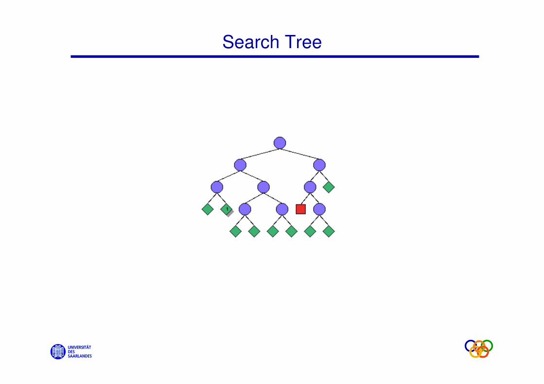
Search Tree

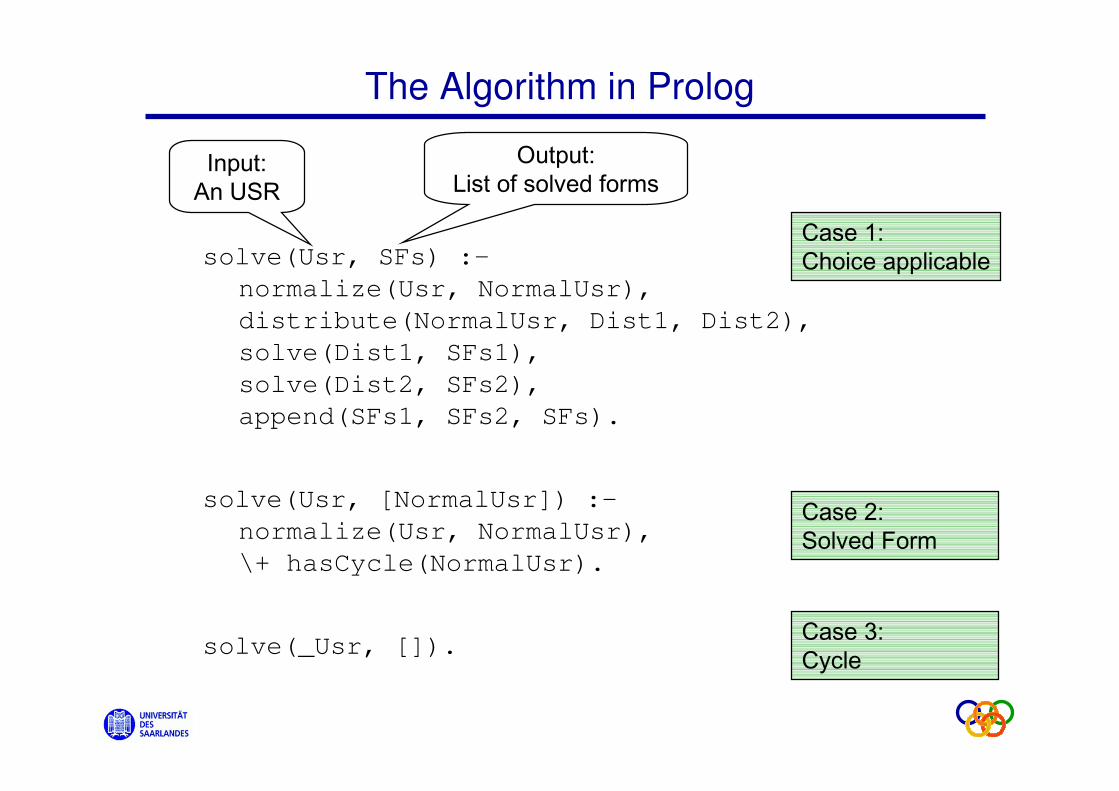
The Algorithm in Prolog

solve(Usr, SFs) :-

normalize(Usr, NormalUsr),

distribute(NormalUsr, Dist1, Dist2),

solve(Dist1, SFs1),

solve(Dist2, SFs2),

append(SFs1, SFs2, SFs).

solve(Usr, [NormalUsr]) :-

normalize(Usr, NormalUsr),

\+ hasCycle(NormalUsr).

solve(_Usr, []).

Input:An USR

Output:List of solved forms

Case 1:Choice applicable

Case 2:Solved Form

Case 3:Cycle

Subroutines

u The algorithm uses some other predicates. These are all available on the course website.

u Here we look at

– distribute

– elimRedundancy

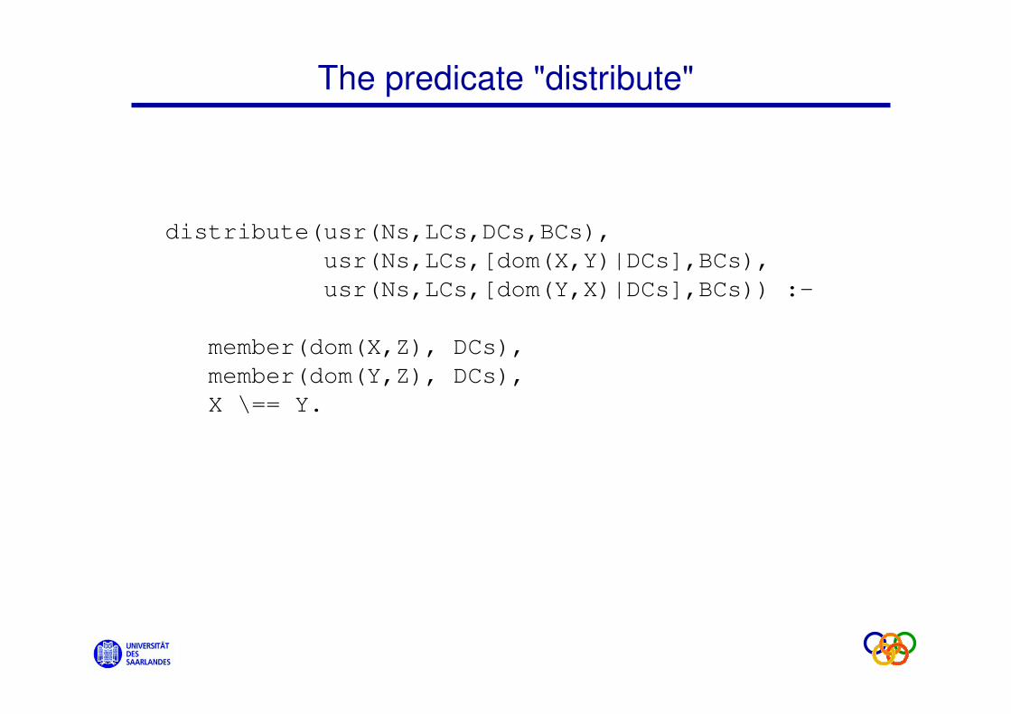
The predicate "distribute"

distribute(usr(Ns,LCs,DCs,BCs),

usr(Ns,LCs,[dom(X,Y)|DCs],BCs),

usr(Ns,LCs,[dom(Y,X)|DCs],BCs)) :-

member(dom(X,Z), DCs),

member(dom(Y,Z), DCs),

X \== Y.

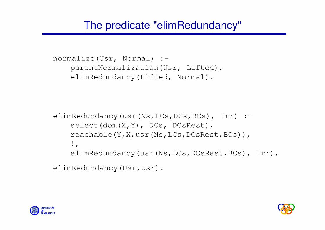
The predicate "elimRedundancy"

normalize(Usr, Normal) :-

parentNormalization(Usr, Lifted),

elimRedundancy(Lifted, Normal).

elimRedundancy(usr(Ns,LCs,DCs,BCs), Irr) :-

select(dom(X,Y), DCs, DCsRest),

reachable(Y,X,usr(Ns,LCs,DCsRest,BCs)),

!,

elimRedundancy(usr(Ns,LCs,DCsRest,BCs), Irr).

elimRedundancy(Usr,Usr).

A Note on Efficiency

u The implementation is correct, but:

– checking for cycles is not a complete

unsatisfiability test: Search space may be too large.

– Redundancy Elimination, Choice, etc. are

not implemented efficiently.

u Both problems can be solved. Best current implementations enumerate over 100.000

solved forms per second (Bodirsky et al.

2004).

A Note on Formalisms

u Dominance graphs are equivalent to normal dominance constraints (Althaus et al. 03;

Egg et al. 01).

u Hole Semantics (Bos 96) can be encoded into

normal dominance constraints (Koller et al. 03).

u MRS (Copestake et al. 99) can be encoded

into normal dominance constraints (Niehren & Thater 03; Fuchss et al. 04).

Summary

u Semantics construction for dominance graphs:

– use Tuesday's framework

– use interface nodes to combine subgraphs

– clean construction that introduces variables and binders together.

u Solving dominance graphs:

– enumerate solved forms

– driving force is Choice rule

– Prolog implementation very concise

– can be made efficient (not in Prolog)

State of the art in underspecification

u Well-understood formalisms.

u Efficient solvers are available.

u Large-scale grammars that compute

underspecified semantic descriptions are

available: e.g. English Resource Grammar (Copestake & Flickinger, 2000).

u Used, in one form or another, in most major grammars that define semantics.