Day 3B Nonparametrics and Bootstrap - A. Colin...

Day 3BNonparametrics and Bootstrap

c A. Colin CameronUniv. of Calif.- Davis

Frontiers in EconometricsBavarian Graduate Program in Economics

.

Based on A. Colin Cameron and Pravin K. Trivedi (2009,2010),Microeconometrics using Stata (MUS), Stata Press.and A. Colin Cameron and Pravin K. Trivedi (2005),

Microeconometrics: Methods and Applications (MMA), C.U.P.

March 21-25, 2011

c A. Colin Cameron Univ. of Calif.- Davis (Frontiers in Econometrics Bavarian Graduate Program in Economics . Based on A. Colin Cameron and Pravin K. Trivedi (2009,2010), Microeconometrics using Stata (MUS), Stata Press. and A. Colin Cameron and Pravin K. Trivedi (2005), Microeconometrics: Methods and Applications (MMA), C.U.P. )BGPE: Nonparametric / Bootstrap March 21-25, 2011 1 / 28

1. Introduction

1. Introduction

Brief discussion of nonparametric and semiparametric methods andthe bootstrap.

1 Introduction2 Nonparametric (kernel) density estimation3 Nonparametric (kernel) regression4 Semiparametric regression5 Bootstrap6 Stata Commands7 Appendix: Histogram and kernel density estimate


2. Nonparametric (kernel) density estimation Summary

2. Nonparametric (kernel) density estimation

Parametric density estimateI assume a density and use estimated parameters of this densityI e.g. normal density estimate: assume yi � N [µ, σ2 ] and use N [y , s2 ].

Nonparametric density estimate: a histogramI break data into bins and use relative frequency within each binI Problem: a histogram is a step function, even if data are continuous

Smooth nonparametric density estimate: kernel density estimate.

Kernel density estimate smooths a histogram in two ways:I use overlapping bins so evaluate at many more pointsI use bins of greater width with most weight at the middle of the bin.


2. Nonparametric (kernel) density estimation Histogram data example

Formula: bfHIST (x0) = 12Nh ∑N

i=1 1(x0 � h < xi < x0 + h) or

bfHIST (x0) = 1Nh ∑N

i=1

12� 1

�� xi�x0h

�� < 1� .Data example: histogram of lnwage for 175 observations

I Varies with the bin width (or equivalently the number of bins)I Here 30 bins, each of width 2h ' 0.20 so h ' 0.10.

0.2

.4.6

.81

Den

sity

0 1 2 3 4 5natural log of hwage


2. Nonparametric (kernel) density estimation Kernel density data example

Kernel density estimate of f (x0) replaces 1 (A) by kernel K (A) :bf (x0) = 1Nh ∑N

i=1 K� xi�x0

h

�Data example: kernel of lnwage for 175 observations

I Epanechnikov kernel K (z) = 0.75(1� z2)� 1(jz j < 1)I h = 0.07 (oversmooths), 0.21 (default) or 0.63 (undersmooths)

0.2

.4.6

.8kd

ensi

ty ln

hwag

e

0 1 2 3 4 5x

Default Half defaultTwice default


2. Nonparametric (kernel) density estimation Implementation

Implementation

Stata examples areI kdensity y uses defaultsI kdensity y, bw(0.2) manually set bandwidthI kdensity y, normal overlays the N [y , s2 ] densityI hist y, kdensity gives both histogram and kernel estimates

Key is choice of bandwidthI The default can oversmooth: may need to decrease bw()

Less important is choice of kernel: default is Epanechnikov.

Other smooth estimators exist including k-nearest neighbors.But usually no reason to use anything but kernel.


3. Kernel regression Local average estimator

3. Kernel regression: Local average estimator

The regression model is yi = m(xi ) + ui , ui � i.i.d. (0, σ(xi )2).I The functional form m(�) is not speci�ed, so NLS not possible.

If many obs have x = x0 use the average of the y 0i s at xi = x0 :

bm(x0) =�∑i : xi=x0

yi�

/�∑i : xi=x0

1�

=�∑Ni=1 1 (xi = x0) yi

�/�∑Ni=1 1 (xi = x0)

�Instead few values of yi at x = x0 so do local average estimator:

bm(x0) = �∑Ni=1 wi0yi

�/�∑Ni=1 wi0

�I where weights wi0 = w(xi , x0) are largest for xi close to x0.

Evaluate at a variety of points x0 gives regression curve.

Di¤erent methods use di¤erent weight functions wi0 = w(xi , x0)


3. Kernel regression Common nonparametric regression estimators

Common nonparametric regression estimators1. Kernel estimate of m(x0) replaces 1 (xi � x0 = 0) by K

� xi�x0h

�bm(x0) = � 1

Nh ∑Ni=1 K

� xi�x0h

�yi�

/�1Nh ∑N

i=1 K� xi�x0

h

��2. Local linear estimate of bm(x0) minimizes w.r.t. a0 and b0

1Nh ∑N

i=1 K� xi�x0

h

�(yi � a0 � b0(xi � x0))2

I Motivation: Kernel estimate is equivalent to bm(x0) minimizes1Nh ∑Ni=1 K

�xi�x0h

�(yi �m0)2 with respect to m0.

I better on endpoints

3. Lowess (locally weighted scatterplot smoothing)I variation of local linear with variable bandwidth, tricubic kernel anddownweighting of outliers.

4. K-Nearest neighborsI Average the y 0i s for the k x

0i s that are closest to x0


3. Kernel regression Kernel regression data example

Kernel regression with 95% con�dence bands, default Kernel(Epanechnikov) and default bandwidths

I lpoly lnhwage educatn, ci msize(medsmall)

01

23

45

natu

ral lo

g of

hw

age

0 5 10 15 20years of completed schooling 1992

95% CI natural log of hwage lpoly smooth

kernel = epanechnikov, degree = 0, bandwidth = 1.53, pwidth = 2.3

Local poly nomial smooth


3. Kernel regression Di¤erent bandwidths

Kernel regression with three bandwidths: default, half and double.I smoother with larger bandwidth

1.5

22.

53

lpol

y sm

ooth

: nat

ural

log

of h

wag

e

0 5 10 15 20lpoly smoothing grid

Default Half defaultTwice default


3. Kernel regression Compare three methods

Kernel, local linear and lowess with default bandwidthsI graph twoway lpoly y x jj lpoly y x, deg(1) jj lowess y xI kernel erroneously underestimates m(x) at the endpoint x = 17.

1.5

22.

53

0 5 10 15 20

Kernel Local linearlowess


3. Kernel regression Implementation

Implementation

Di¤erent methods work di¤erentlyI Local linear and local polynomial handle endpoints better than kernel.bm(x0) is asymptotically normalI this gives con�dence bands that allow for heteroskedasticity

Bandwidth choice is crucialI optimal bandwidth trades o¤ bias (minimized with small bandwidth)and variance (minimized with large bandwidth)

I theory just says optimal bandwidth for kernel regression is O(N�0.2)I �plug-in�or default bandwidth estimates are often not the bestI so also try e.g. half and two times the default.I cross validation minimizes the empirical mean square error

∑i (yi � bm�i (xi ))2, where bm�i (xi ) is the �leave-one-out" estimate ofbm(xi ) formed with yi excluded.c A. Colin Cameron Univ. of Calif.- Davis (Frontiers in Econometrics Bavarian Graduate Program in Economics . Based on A. Colin Cameron and Pravin K. Trivedi (2009,2010), Microeconometrics using Stata (MUS), Stata Press. and A. Colin Cameron and Pravin K. Trivedi (2005), Microeconometrics: Methods and Applications (MMA), C.U.P. )BGPE: Nonparametric / Bootstrap March 21-25, 2011 12 / 28

4. Semiparametric estimation Motivation

4. Semiparametric estimation

Nonparametric regression is problematic when more than one regressorI in theory can do multivariate kernel regressionI in practice the local averages are over sparse cellsI called the �curse of dimensionality�

Semiparametric methods place some structure on the problemI parametric component for part of the modelI nonparametric component that is often one dimensional


4. Semiparametric estimation Leading examples

Leading semiparametric examples

Partially linear model

E[yi jxi , zi ] = x0iβ+ λ(zi )

I Estimate λ(�) nonparametrically and ideallypN(bβ� β)

d! N [0,V]

Single-index modelE[yi jxi ] = g(x0iβ)

I Estimate g(�) nonparametrically and ideallypN(bβ� β)

d! N [0,V]I Can only estimate β up to scale in this modelI Still useful as ratio of coe¢ cients equals ratio of marginal e¤ects in asingle-index models

Generalized additive model

E[yi jxi ] = g1(x1i ) + � � �+ gK (xKi )


5. Bootstrap Estimate of standard error

5. Bootstrap estimate of standard error

Basic idea is view f(y1, x1), ..., (yN , xN )g as the population.Then obtain B random samples from this population

I Get B estimates bθ1, ...,bθS .I Then estimate Var[bθ] using the usual standard deviation of the Bestimates

bV[bθ] = 1B�1 ∑B

b=1(bθs � bθ)2, where bθ = 1

B ∑Bb=1

bθb .I Square root of this is called a bootstrap standard error.

To get B di¤erent samples of size N we resample with replacementfrom f(y1, x1), ..., (yN , xN )g

I In each bootstrap sample some original data points appear more thanonce while others not appear at all.


5. Bootstrap Regression application

Regression application

Data: Doctor visits (count) and chronic conditions. N = 50.

chronic 50 .28 .4535574 0 1age 50 4.162 1.160382 2.6 6.2

docvis 50 4.12 7.82106 0 43

Variable Obs Mean Std. Dev. Min Max

. summarize

Sorted by:

chronic byte %8.0g = 1 if a chronic conditionage float %9.0g Age in years / 10docvis int %8.0g number of doctor visits

variable name type format label variable labelstorage display value

size: 750 (99.9% of memory free)vars: 3 16 Apr 2010 10:32obs: 50

Contains data from musbootdata.dta


5. Bootstrap Standard error estimation

Bootstrap standard errors after Poisson regression

Use option vce(boot)I Set the seed!I Set the number of bootstrap repetitions!

_cons 1.031602 .3497212 2.95 0.003 .3461607 1.717042chronic .9833014 .5253149 1.87 0.061 -.0462968 2.0129

docvis Coef. Std. Err. z P>|z| [95% Conf. Interval]Observed Bootstrap Normal-based

Log likelihood = -238.75384 Pseudo R2 = 0.0917Prob > chi2 = 0.0612Wald chi2(1) = 3.50Replications = 400

Poisson regression Number of obs = 50

. poisson docvis chronic, vce(boot, reps(400) seed(10101) nodots)

. * Compute bootstrap standard errors using option vce(bootstrap) to

Bootstrap se = 0.525 versus White robust se = 0.515.


5. Bootstrap Standard error estimation

Results vary with seed and number of reps

legend: b/se

0.39545 0.32575 0.34885 0.34467_cons 1.03160 1.03160 1.03160 1.03160

0.47010 0.50673 0.53479 0.51549chronic 0.98330 0.98330 0.98330 0.98330

Variable boot50 boot50~f boot2000 robust

. estimates table boot50 boot50diff boot2000 robust, b(%8.5f) se(%8.5f)

. estimates store robust

. quietly poisson docvis chronic, vce(robust)

. estimates store boot2000

. quietly poisson docvis chronic, vce(boot, reps(2000) seed(10101))

. estimates store boot50diff


. estimates store boot50


. * Bootstrap standard errors for different reps and seeds


5. Bootstrap Leading uses of bootstrap standard errors

Leading uses of bootstrap standard errors

Sequential two-step m-estimatorI First step gives bα used to create a regressor z(bα)I Second step regresses y on x and z(bα)I Do a paired bootstrap resampling (x , y , z)I e.g. Heckman two-step estimator.

2SLS estimator with heteroskedastic errors (if no White option)I Paired bootstrap gives heteroskedastic robust standard errors.

Functions of other estimates e.g. bθ = bα� bβI replaces delta methodI Clustered data with many small clusters, such as short panels.

F Then resample the clusters.F But be careful if model includes cluster-speci�c �xed e¤ects.

For these in Stata need to use pre�x command bootstrap:


5. Bootstrap General algorithm

The bootstrap: general algorithm

A general bootstrap algorithm is as follows:I 1. Given data w1, ...,wN

F draw a bootstrap sample of size N (see below)F denote this new sample w�1 , ...,w

�N .

I 2. Calculate an appropriate statistic using the bootstrap sample.Examples include:

F (a) estimate bθ� of θ;F (b) standard error sbθ� of estimate bθ�F (c) t�statistic t� = (bθ� � bθ)/sbθ� centered at bθ.

I 3. Repeat steps 1-2 B independent times.

F Gives B bootstrap replications of bθ�1 , ...,bθ�B or t�1 , . . . , t�B or .....

I 4. Use these B bootstrap replications to obtain a bootstrapped versionof the statistic (see below).


5. Bootstrap Implementation

ImplementationNumber of bootstraps: B high is best but increases computer time.

I CT use 400 for se�s and 999 for tests and con�dence intervals.I Defaults are often too low. And set the seed!

Various resampling methodsI 1. Paired (or nonparametric or empirical dist. func.) is most common

F w�1 , ...,w�N obtained by sampling with replacement from w1, ...,wN .

I 2. Parametric bootstrap for fully parametric models.F Suppose y jx � F (x, θ0) and generate y �i by draws from F (xi ,bθ)

I 3. Residual bootstrap for regression with additive errorsF Resample �tted residuals bu1, ..., buN to get (bu�1 , ..., bu�N ) and form new(y �1 , x1), ..., (y

�N , xN ).

Need to resample over i.i.d. observationsI resample over clusters if data are clustered

F But be careful if model includes cluster-speci�c �xed e¤ects.

I resample over moving blocks if data are serially correlated.


5. Bootstrap Asymptotic re�nement

Asymptotic re�nement

The simplest bootstraps are no better than usual asymptotic theoryI advantage is easy to implement, e.g. standard errors.

More complicated bootstraps provide asymptotic re�nementI this may provide a better �nite-sample approximation.

Conventional asymptotic tests (such as Wald test).I α = nominal size for a test, e.g. α = 0.05.I Actual size= α+O(N�1/2).

Tests with asymptotic re�nementI Actual size= α+O(N�1).I asymptotic bias of size O(N�1) < O(N�1/2) is smaller asymptotically.I But need simulation studies to con�rm �nite sample gains.

F e.g. if N = 100 then 100/N = O(N�1) > 5/pN = O(N�1/2).


5. Bootstrap Asymptotically Pivotal Statistic

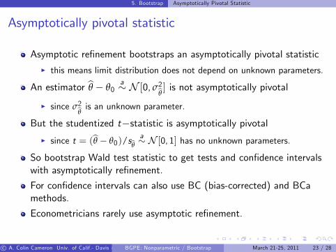
Asymptotically pivotal statistic

Asymptotic re�nement bootstraps an asymptotically pivotal statisticI this means limit distribution does not depend on unknown parameters.

An estimator bθ � θ0a� N [0, σ2bθ ] is not asymptotically pivotal

I since σ2bθ is an unknown parameter.But the studentized t�statistic is asymptotically pivotal

I since t = (bθ � θ0)/sbθ a� N [0, 1] has no unknown parameters.

So bootstrap Wald test statistic to get tests and con�dence intervalswith asymptotically re�nement.

For con�dence intervals can also use BC (bias-corrected) and BCamethods.

Econometricians rarely use asymptotic re�nement.


5. Bootstrap Con�dence intervals

(BCa) bias-corrected and accelerated confidence interval(BC) bias-corrected confidence interval(P) percentile confidence interval(N) normal confidence interval

.3794897 1.781907 (BCa)

.2578293 1.649789 (BC)

.2177235 1.598568 (P)_cons 1.0316016 -.0503223 .35257252 .3405721 1.722631 (N)

-.0215526 2.181476 (BCa)-.0820317 2.100361 (BC)-.1316499 2.076792 (P)

chronic .98330144 -.0244473 .54040762 -.075878 2.042481 (N)

docvis Coef. Bias Std. Err. [95% Conf. Interval]Observed Bootstrap

Replications = 999Poisson regression Number of obs = 50

. estat bootstrap, all

. quietly poisson docvis chronic, vce(boot, reps(999) seed(10101) bca)

. * Bootstrap confidence intervals: normal-based, percentile, BC, and BCa

(N) is observed coe¢ cient � 1.96 � bootstrap s.e.

(P) is 2.5 to 97.5 percentile of the bootstrap estimates bβ�1, ..., bβ�B .(BC) and (BCa) have asymptotic re�nement.


5. Bootstrap Bootstraps can fail

Bootstrap failure

The following are cases where standard bootstraps failI so need to adjust standard bootstraps.

GMM (and empirical likelihood) in over-identi�ed modelsI For overidenti�ed models need to recenter or use empirical likelihood.

Nonparametric Regression:I Nonparametric density and regression estimators converge at rate lessthan root-N and are asymptotically biased.

I This complicates inference such as con�dence intervals.

Non-Smooth Estimators: e.g. LAD.


6. Stata Commands

6. Stata commands

Command kernel does kernel density estimate.

Command lpoly does several nonparametric regressionsI kernel is defaultI local linear is option degree(1)I local polynomial of degree p is option degree(p)

Command lowess does Lowess.

Stata has no built-in commands for the semiparametric estimatorsI These methods are not easy to automate as no easy way to automatebandwidth choice and treatment of outliers.

For bootstrap use option ,vce(boot) or command bootstrap:I set the seed!!


7. Appendix Histogram estimate

7. Appendix: Histogram estimate

A histogram is a nonparametric estimate of the density of yI break data into bins of width 2hI form rectangles of area the relative frequency = freq/NI the height is freq/2Nh (then area = (freq/2Nh)� 2h = freq/N).

Use freq = ∑Ni=1 1(x0 � h < xi < x0 + h)

I where indicator function 1(A) equals 1 if event A happens and equals0 otherwise

The histogram estimate of f (x0), the density of x evaluated at x0, is

bfHIST (x0) = 12Nh ∑N

i=1 1(x0 � h < xi < x0 + h)

= 1Nh ∑N

i=1

12� 1

�� xi�x0h

�� < 1� .c A. Colin Cameron Univ. of Calif.- Davis (Frontiers in Econometrics Bavarian Graduate Program in Economics . Based on A. Colin Cameron and Pravin K. Trivedi (2009,2010), Microeconometrics using Stata (MUS), Stata Press. and A. Colin Cameron and Pravin K. Trivedi (2005), Microeconometrics: Methods and Applications (MMA), C.U.P. )BGPE: Nonparametric / Bootstrap March 21-25, 2011 27 / 28

7. Appendix Kernel density estimate

Appendix: Kernel density estimate

Recall bfHIST (x0) = 1Nh ∑N

i=112 � 1

�� xi�x0h

�� < 1�Replace 1 (A) by a kernel functionKernel density estimate of f (x0), the density of x evaluated at x0, is

bf (x0) = 1Nh ∑N

i=1 K� xi�x0

h

�I K (�) is called a kernel functionI h is called the bandwidth or window width or smoothing parameter h

Example is Epanechnikov kernelI K (z) = 0.75(1� z2)� 1(jz j < 1)I more weight on data at center. less weight at end

More generally kernel function must satisfy conditions includingI Continuous, K (z) = K (�z),

RK (z)dz = 1,

RK (z)dz = 1,

tails go to zero.


Day 3B Nonparametrics and Bootstrap - A. Colin...

Documents

Transcript of Day 3B Nonparametrics and Bootstrap - A. Colin...