David Preece - L6 Geography - · PDF fileDavid Preece - L6 Geography 1 AN INVESTIGATION IN TO...

David Preece - L6 Geography

1

AN INVESTIGATION IN TO THE DOWNSTREAM FLOW VARIABLES

OF THE RIVER CLYWEDOG, WREXHAM

by

David Preece


2

King Edward VI Camp Hill School For Boys'

Abstract

AN INVESTIGATION IN TO THE DOWNSTREAM FLOW

VARIABLES OF THE RIVER CLYWEDOG, WREXHAM.

by David Preece

This piece of work is intended as an investigation in to the variation in

downstream changes in river channel characteristics on the River Clywedog. The

work is carried out in partial fulfillment of module GGO2 Section A, which

requires the completion of a model investigation.

The question is to be investigated derives from knowledge of river channel

process gained through class work and relevant research using secondary sources.


3

TABLE OF CONTENTS

Chapter 1 - Determining the Variables 1.1. Introduction........................................................................................................... 6 1.2. Depth...................................................................................................................... 6 1.3. Width ...................................................................................................................... 7 1.4. Cross Sectional Area ............................................................................................ 9 1.5. Wetted Perimeter.................................................................................................. 9 1.6. Hydraulic Radius................................................................................................. 10 1.7. Gradient ............................................................................................................... 10 1.8. Velocity................................................................................................................. 10 1.9. Discharge ............................................................................................................. 11

Chapter 2 - Evaluation of Secondary Sources ............................................................. 13 Chapter 3 - Location of the Study

3.1. Location ............................................................................................................... 15 3.2. Grid References .................................................................................................. 15 3.3. Choice of Site ...................................................................................................... 15 3.4. Site Grid References .......................................................................................... 15

Chapter 4 - Primary Data Collection - Methodology

4.1. Introduction......................................................................................................... 18 4.2. Choice of Sampling Points ............................................................................... 18 4.3. Measuring Width ................................................................................................ 18 4.4. Measuring Depth................................................................................................ 18 4.5. Measuring Segment Velocity ............................................................................ 19 4.6. Maintaining Accuracy ........................................................................................ 20

Chapter 5 - Data Presentation ........................................................................................ 21 Chapter 6 - Data Analysis

6.1. Gradient Analysis ............................................................................................... 29 6.2. Long Profile Analysis......................................................................................... 29 6.3. Cross Sectional Area Analysis .......................................................................... 29 6.4. Velocity Analysis................................................................................................. 30 6.5. Discharge Analysis ............................................................................................ 30 6.6. Analysis of the testing of Leopold and Maddocks flow variables ............. 31

Chapter 7 - Evaluation of Results, Techniques and Location of the Study ........... 33 Chapter 8 - List of Sources.............................................................................................. 36


4

LIST OF FIGURES

Number Page Figure 1 - Graph of Distance Downstream against Depth 7

Figure 2 - Graph of Distance Downstream against Width 8

Figure 3 - Graph of Distance Downstream against Velocity 11

Figure 4 - Graph of Distance Downstream against Discharge 12

Figure 5 - Vertical Velocity Profile 19

Figure 6 - Table of Data 21

Figure 7 - Gradient Downstream 22

Figure 8 - Long Profile of the Studied Section 23

Figure 9 - Downstream Changes in Cross Sectional Area 24

Figure 10 - Downstream Changes in Velocity 25

Figure 11 - Downstream Changes in Discharge 26

Figure 12 - Discharge and Cross Sectional Area 27

Figure 13 - Discharge and Velocity 28

Figure 14 - Photograph of Site No.2 29

Figure 15 - Photograph of Site No.4 30

Figure 16 - Velocity without human management 31

Figure 17 - Discharge without human management 31


6

C h a p t e r 1

DETERMINING THE VARIABLES

1.1. Introduction This investigation was started with a consideration of all possible variables which could occur over a 1-2 km stretch of the Clywedog. Because of this relatively short distance, it was decided the long profile would not form a key part of the investigation, though it would form part of the background material.

1.2. Depth The first variable to be considered was the channel depth. Defined as ‘the vertical distance from the water surface to the bed of the channel’ 1, the channel depth is an easily considered variable. It will also serve a useful purpose in estimating potential energy of a river, since geographical theory tells us that upper section rivers will incise narrow channels to lose potential energy as rapidly as possible; “The thermodynamic principle of least work would give a waterfall from source to sea level. All the energy would change instantly from potential to kinetic” 2 The section of the Clywedog which we are studying is in the middle section, so we would expect some combination of incision and meander.

1 From 'Process and Landform - Conceptual Framework in Geography' by Clowes and Comfort. First edition,

published by Oliver and Boyd.

2 From 'Process and Landform - Conceptual Framework in Geography' by Clowes and Comfort. First edition, published by Oliver and Boyd


7

The depth will be related to this. We would expect mean depth to increase downstream, and the secondary sources support this view. According to Edwards 3, the downstream depth of the Clywedog increases. The chart shows the values Edwards obtained, along with a trendline, which indicates a slowly increasing depth with distance downstream

This work is also supported by Leopold and Maddocks. In 1953, they published their work on the ‘hydraulic geometry’ of downstream flow variables, based on records of streams in the central and south-west USA. Their work will be referred to later in reference to both width and velocity. For depth, they obtained the relationship;

D ∝ Q0.4 i.e. depth increases nearly as the square root of discharge. Hence, since depth can be measured without overt difficulty, it will be one of the variables to be investigated downstream. As such, it will form part of the later sections of the data to be recorded.

1.3. Width The second considered variable was width. Defined as ‘the length along this line [perpendicular across the river flow] from the water’s edge to the opposite edge’ 4. Like the depth, the width is easily measured, and has confirmation by the same

3 Edwards, M. Unpublished dissertation on the downstream flow variables of the River Clywedog, 1979.

Station intervals at approx. 500-750m.

4 Adapted from 'Process and Landform - Conceptual Framework in Geography' by Clowes and Comfort. First edition, published by Oliver and Boyd.

Downstream Channel Variables on the R.Clywedog, after Edwards M, 1979 (unpubl.)

y = 0.0066x + 0.075

00.05

0.10.150.2

0.250.3

0.350.4

0 5 10 15 20 25 30

Station Number

Dep

th (

m)


8

secondary sources as before. Leopold and Maddock established the relationship between width and discharge to be set as

Width ∝ √Q i.e. Width increases as the square root of discharge. In a sense, Leopold and Maddocks’ work is unsuitable to use for this investigation, since it explores the relationship between variables and discharge. In this investigation, discharge will be one of the variables under examination, and thus we can explore the interaction of variables to the modelled conditions of Leopold and Maddocks’ work. Altogether more directly suitable is the work of Edwards, who obtained the

results shown below for her width values downstream. Despite the use of Edwards’ data, the trendline shows an almost random scattering of widths downstream with a slight tendency to increase. The correlation value for this data is given as 0.234, which indicates a very slight positive correlation. The manifest flaw in measuring an increase in width downstream with fixed station intervals, as Edwards did, is that the cross section and width can change very rapidly in a short distance because of meanders, channels and the geology of the area. Thus, an irregular data set is obtained. Ideally, channel shape should be compared with channel shape, so meanders should be compared downstream to see how the width of the meander changes. However, this is not possible to do with the limited resources available. Using only a short stretch of the Clywedog, we can measure width and depth, and by inspecting the profile, can determine the position of the cross section on the river, i.e. on a meander or an incised channel. This will reduce the error seen in

Downstream Channel flow Variables on the R.Clywedog after Edwards M, 1979 (unpubl.)

01

234

56

78

0 5 10 15 20 25 30

Station Number

Wid

th (

m)


9

the work of Edwards, and produce a reasonable value for width increase downstream as a variable to be investigated.

1.4. Cross Sectional Area. The next variable which follows on logically from width and depth is the cross sectional area. The cross sectional area is self explanatory as the area of the cross section. It can be read off an accurately drawn profile map, or alternatively, a comparable result can be produced by taking the mean depth, and multiplying it by the width. It follows logically, then, that Leopold and Maddocks’ work can be mathematically extended to give us a relationship between cross sectional area and discharge. Hence;

W ∝ Q 4/10 and D ∝ Q ½ We also know that C (Cross Sectional Area) = W x D Thus;

C ∝ Q 4/10 x Q ½

So C ∝ Q 9/10

This gives another relationship to test in addition to the main hypothesis.

1.5. Wetted Perimeter Once again, the discussion of one variable leads on to another. If we have a profile plotted, then we can evidently test the relationship between wetted perimeter and distance downstream. Defined as ‘the total length of the bed and bank sides in contact with the water in the channel’ 5, the wetted perimeter will naturally vary with width and depth. Theory tells us that the cross section of a river increases in size with distance downstream, and it follows that the wetted perimeter will do so also. However, despite the ability to investigate the wetted perimeter, it is not enough to be investigated as a pure variable. The value of the wetted perimeter is part of the explanation for varying velocities because of friction, but this is more related to a product of wetted perimeter than to wetted perimeter as a sole variable.

5 From 'Geography - An Integrated Approach' by David Waugh. 3rd edition, published by Nelson


10

1.6. Hydraulic Radius The wetted perimeter leads on naturally to the hydraulic radius, of which it forms a part. The hydraulic radius is defined as ‘the ratio between the cross section of a river channel and the length of its wetted perimeter’ 6. It measures what is effectively the efficiency of the river. Since theory tells us that the slowest flow will be on the areas where the water comes in to contact with the bed and banks, the amount of water which is not in contact with the bed and banks is a useful measure of effectiveness. This will be a far more useful variable to record from the computer data, as it will explain much more effectively the effect of friction than the wetted perimeter will.

1.7. Gradient The next variable to be considered is gradient. Although it is worth noting, in case of a steep gradient which alters the flow pattern, it will not be sufficiently noticeable to change the flow of the river.

1.8. Velocity Finally on to the last measurable variable. The velocity of the river, which is defined as ‘the rate of flow of the river’ 7, is to be measured in defined segments of 0.5 m across the width. We can thus obtain a picture of how the river flows at points across the channel, to test conventional theory, and also measure the change in velocity downstream. It would be conventional to assume that since the river has lost Kinetic Energy wasted through friction, the river would be flowing more slowly than at the start when it had large amounts of PE. However, it is believed that due to increased efficiency at greater depth, the river velocity actually increases downstream.8 Once again, Edwards’ work is used as a reference, and it would appear that the correlation between distance downstream and velocity has a precedent in other research. This does not, of course, mean we will find the same in the investigation, but it is worth noting. Edwards’ work shows a slight increase in velocity over the length of the whole river, and it is possible that we will not find such an increase, using a much shorter and far more similar section of land than the whole river. This cannot be helped, and there is no way to do this differently without more resources than have been allocated. 6 From 'Geography - An Integrated Approach' by David Waugh. 3rd edition, published by Nelson

7 Adapted from 'Geography - An Integrated Approach' by David Waugh. 3rd edition, published by Nelson

8 Summarised from 'Process and Landform - Conceptual Framework in Geography' by Clowes and Comfort. First edition, published by Oliver and Boyd.


11

Leopold and Maddocks’ work also gives a relationship between velocity and discharge. According to them,

V ∝ Q 0.1 i.e. velocity increases as the tenth root of discharge. It seems unfortunate that Leopold and Maddocks did not link distance downstream and discharge for a mathematical equation.

1.9. Discharge All of the variables discussed nevertheless need linking together under a generic entity. It seems that testing the relationship between distance downstream and discharge is the most appropriate investigation to be carried out. Discharge, which is defined as ‘the volume of water passing a point in a given time, dependent on the velocity of the river and the size of the channel at that point’9 can be measured using the variables of width, depth and velocity described earlier. It can then be explained and compared using hydraulic radius. According to theory, the discharge should increase as cross section and velocity increase downstream. Edwards’ work shows a distinct correlation (0.73) between distance downstream and discharge.

9 Adapted from 'Process and Landform - Conceptual Framework in Geography’ by Clowes and Comfort.

First edition, published by Oliver and Boyd

Downstream flow Variables in the R.Clywedog after Edwards M, 1979 (unpubl.)

y = 0.0092x + 0.2451

0

0.1

0.2

0.3

0.4

0.5

0.6

0.7

0 5 10 15 20 25 30

Station Number

Vel

oci

ty (

m/s

)


12

This is supported by the theory; since both cross sectional area and velocity increase, then discharge must also increase. This correlation is clear, and could almost be traced back to the origin.

It seems that the variable to be investigated is the relationship between discharge and distance downstream.

Allowing for the short distance to be covered, I think that there will be an increase, though not necessarily a large increase. This hypothesis is supported by the work of Leopold and Maddocks with reference to streams in general, and more pleasingly, by the work of Edwards on the Clywedog in 1979. It is an easily measurable variable, but only by combining other variables to be measured, namely the width, depth and segment velocity.

Downstream channel Variables on the R.Clywedog after Edwards M, 1979 (unpubl)

0

0.1

0.2

0.3

0.4

0.5

0.6

0.7

0 5 10 15 20 25 30


13

C h a p t e r 2

EVALUATION OF SECONDARY SOURCES

Whilst it is fundamental to base work on theoretical rational which can only be obtained from available secondary sources, it does not necessarily mean that the secondary sources are sound practical guides, or indeed accurate in any way. The work of Chezy in 1768 is useful in telling us that the question of river flow variables were being considered in the 18th Century, but is of little other use. Manning’s work is also of this nature, although his coefficient of bed roughness would be suitable for testing in a study at a higher level, and would provide interesting analysis, particularly on the definitions of categories. Initially it would appear that far more suitable for the purposes of this study is the work of Edwards (1979). Despite the relatively limited time available, Edwards has produced a piece investigating the downstream flow variables of the Clywedog. The use, therefore, is evident in that it is the same river as studied here. We only have Edwards’ results available. Since the thesis is unpublished, we cannot access the methodology, nor can we assess the location factors which she may or may not have considered. Without the benefit of this knowledge, an brief assessment of her work can be done, which will relate to how useful the work is. Of an elementary nature, the work was probably carried out in a very small group, perhaps a maximum of two. The difficulty of measuring width, depth, and segment velocity with such a small number is self evident. It is hard to hold a ranging pole, a tape measure taut and simultaneously record data, let alone measure velocity as well. But this is not the only question mark over her work. It seems that she may have had difficulty with access to parts of the river. The spacing intervals of 500 - 750 metres do not imply accuracy. It makes it hard to plot data against a long profile if the actual distance from the start of the study is unknown. The relatively small number of cross section is also questionable. Would this really constitute accuracy? Allowing for time constraints, perhaps more could have been done. Edwards work only covers perhaps 15-20 km.


14

Referring once again to the lack of data in terms of the remainder of the study, perhaps this would have cleared up some of the questions which remain unanswered. For example, what was the overall objective of the study? How did Edwards evaluate her own work? What were her conclusions? What secondary sources were used to provide theoretical rationale? More importantly, Edwards work is not of the standard to be used as a ‘source’. It is merely a study which assists us in evaluating the variables. It has not made the conceptual transition to be classed with Leopold and Maddock and Manning as a microcosmic work. The work of Leopold and Maddock is recognised as one of the classics in mathematical fluvial analysis. Their variables and relationships to discharge have been proven, within the bounds of experimental error, to be universally applicable. Their variables have the ability to be manipulated to provide other variables, for example see section 1.4. This extends the possibility for further work and testing of variables.


15

C h a p t e r 3

LOCATION OF STUDY

3.1. Location The study of the river is to take place in the lower middle course, where it crosses Erddig Country Park.

3.2. Grid References The River Clywedog, the river to be studied, flows from Esclusham, GR. 228 49710 over approximately 22 ½ kilometres before it joins the River Dee at GR. 407 473 11. It’s catchment area encompasses the area for 5 kilometres south and west of Wrexham.

3.3. Choice of Site This site has been chosen for several reasons. Firstly, it is on open access National Trust land, and therefore easily accessible. Secondly, it is within easy driving distance of our study base in Chester, which means that the whole field work can be completed in one day. Thirdly, the river exhibits some changes within a short section. Not only does it widen as it spreads on to an unconstricted floodplain, but it is also joined by a tributary, the Black Brook, which will contribute to its discharge and load. This should give a wide variety of channel forms, meaning that we can use this river as a microcosm for rivers generally. It can be seen on the map over leaf.

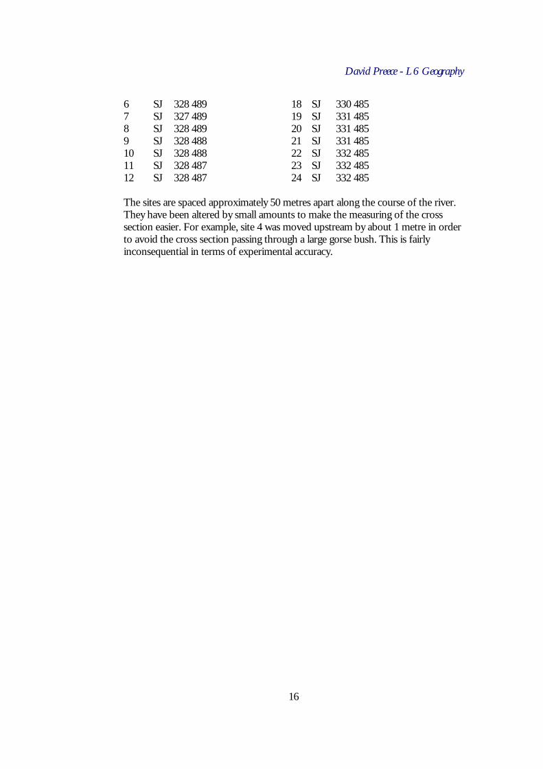
3.4. Site Grid References The Grid References for each site, using an OS 1:25000 Map are; 1 SJ 326 492 13 SJ 328 488 2 SJ 327 491 14 SJ 328 487 3 SJ 328 491 15 SJ 328 486 4 SJ 328 490 16 SJ 329 486 5 SJ 328 490 17 SJ 330 485

10 Reference given is the source of the river’s principal tributary, the Aber Sychnnat, from Ordnance Survey

1:50 000 series Sheet 117, Edition 8 GSGS.

11 Reference from Ordnance Survey 1:50 000 series, Sheet 117, Edition 8 GSGS.


16

6 SJ 328 489 18 SJ 330 485 7 SJ 327 489 19 SJ 331 485 8 SJ 328 489 20 SJ 331 485 9 SJ 328 488 21 SJ 331 485 10 SJ 328 488 22 SJ 332 485 11 SJ 328 487 23 SJ 332 485 12 SJ 328 487 24 SJ 332 485 The sites are spaced approximately 50 metres apart along the course of the river. They have been altered by small amounts to make the measuring of the cross section easier. For example, site 4 was moved upstream by about 1 metre in order to avoid the cross section passing through a large gorse bush. This is fairly inconsequential in terms of experimental accuracy.


18

C h a p t e r 4

PRIMARY DATA COLLECTION - METHODOLOGY

4.1. Introduction As discussed in Chapter 1, the measurement of the discharge cannot be done immediately. Discharge must be calculated from other variables, each of which is eminently measurable. In Chapter 1, it was decided that the variables to measure were width, depth, and segment velocity. Using computer software, we could then model the section and thus the discharge.

4.2. Choice of Sampling points The choice of sampling points was a relatively simple one. Starting at the confluence of the Clywedog and the Black Brook, and moving upstream, we measured approximately 50 metre intervals along the stream itself. This technique was flawed in that we used paces to measure approximately a metre. In addition, the paces were taken through water. This meant that the actual distance upstream was probably only 80% of the estimated distance, which puts the sample separations at around 40m. In addition, if the sample distance resulted in an awkward position to take readings from, then it was altered for ease of data recording. The experimental error resulting from this is only very small.

4.3. Measuring Width The process of recording a section result is complex in that it involves many measurements, but these themselves are simple to do. This first task involves setting up range pole either side of the channel. Bearing in mind the definition of width, the range poles were taken to the water’s edge rather than the limits of the river cliff or the deposition found on the inside of the meander bend, for example. Once the range poles were set up, a measuring tape was taken across the width, perpendicular to the bank, and the width recorded.

4.4. Measuring Depth The tape had 0.5 metre intervals marked on it, and at each of these, the depth and segment velocity were recorded. The dry depth was measured using a metre rule which was placed in line with the current flow, and the distance from the tape to the water’s surface measured. Where the water flow was turbulent, then the basal surface depth was used. The metre rule was then placed perpendicular to the bed, and the wet depth was measured, again using the same technique. These values were recorded as separate entities.


19

4.5. Measuring Segment Velocity The segment velocity was recorded using a flow meter. This comprises of an impeller and a meter which records the number of turns the impeller makes in one minute. The length of time is controlled by a switch, which activates the counter when desired. The number can then be plotted on a conversion graph to give approximate river velocity. The impeller is placed at approximately 60% of the depth, to avoid the friction and turbulence caused by the bed or the surface of the water. This is explained in this extract; “the profile of the laminar flow is a smooth parabola curving up from th stream bed ….. in these areas velocity is low because of friction between the static bed and the moving water … the friction is greatest at the edges of the channel, which are therefore the zones of slowest flow” 12 The expression of this flow pattern in a graph is perhaps the best way to show where the impeller should be placed.

Extracted from 'Process and Landform - Conceptual Framework in Geography' by Clowes and Comfort. First edition, published by Oliver and Boyd

This graph shows an idealised profile which results in our use of the figure of 60% for depth. The flow meter is positioned upstream of the recorder, and the impeller allowed to move for a short while before the time is started. For 1 minute, the counter records the number of complete turns that the impeller makes. The number is then compared to a pre-prepared graph, which converts the number of turns in to an approximate value for velocity in metres per second.

12 Extracted from 'Process and Landform - Conceptual Framework in Geography' by Clowes and Comfort.

First edition, published by Oliver and Boyd. See p.93 for full version.

Velocity Profile

0

1

2

3

0 0.05 0.1 0.15 0.2 0.25 0.3

Velocity (m/s)

Dep

th (

m)

Surface Velocity (Vs)

0.6 depth

Mean Velocity (0.8 Vs)


20

4.6. Maintaining Accuracy To ensure accuracy throughout, the apparatus was kept constant. The measurements were always taken from the far bank and measured in towards the near bank. The ranging poles were always planted at the water’s edge, rather than that of the bank. In addition the members of the recording team performed the same task throughout, ensuring consistency and an increasing level of expertise in the specialist field.


21

C h a p t e r 5

DATA PRESENTATION

The following results were obtained by the groups on each of the 24 sites.

Site No. Wetted Perimeter

Area Hydraulic Radius

Mean Velocity

Discharge

1 3.53 0.81 0.23 0.56 0.42 2 5.06 2.43 0.48 0.09 0.23 3 2.05 0.51 0.25 0.94 0.39 4 4.52 0.82 0.18 0.54 0.46 5 6.56 0.90 0.14 0.06 0.05 6 3.02 0.56 0.19 0.26 0.10 7 3.54 0.60 0.17 0.16 0.10 8 4.55 0.90 0.20 0.15 0.14 9 7.51 0.68 0.09 0.26 0.17 10 4.02 0.66 0.16 0.29 0.14 11 5.02 0.68 0.14 0.27 0.22 12 5.00 0.77 0.15 0.27 0.20 13 6.15 2.67 0.43 0.16 0.43 14 5.05 0.77 0.15 0.75 0.51 15 4.59 1.34 0.29 0.14 0.13 16 7.09 1.04 0.15 0.32 0.30 17 6.74 1.77 0.26 0.06 0.10 18 5.56 1.78 0.32 0.07 0.13 19 6.03 0.84 0.14 0.22 0.17 20 8.04 1.24 0.15 0.15 0.19 21 6.59 2.30 0.35 0.03 0.07 22 7.55 2.07 0.27 0.03 0.07 23 7.09 2.88 0.41 0.02 0.06 24 7.61 3.7 0.49 0.01 0.04

Table of Raw Data.

The following graphs have all been produced using the data above, and the manipulation of these results in Microsoft Excel.


29

C h a p t e r 6

DATA ANALYSIS

6.1. Gradient Analysis Despite the dramatic looking graph, Chart 1, the variation in the gradient is only 3° at maximum. This is fairly consistent with the mid section of a river, with a fairly shallow slope. The accuracy of the gradient is broadly debatable, but the true values should not be too far from the values given here. The main purpose of the gradient measure is to calculate long profile, saving interpolation from contour lines on the map.

6.2. Long Profile Analysis The Long Profile shows the energy levels of the river, with zero at the end of the section studied. While the graph looks relatively concordant with textbook examples, it is worth remembering that the scale is quite small. Energy calculations can be done to work out the true theoretical maximum velocity of the river without friction, which provides interesting comparison with the true velocity. The long profile also would be interesting to match against the velocity of the river, to see if the flat areas have lowest velocity, and the steep areas have the highest velocity.

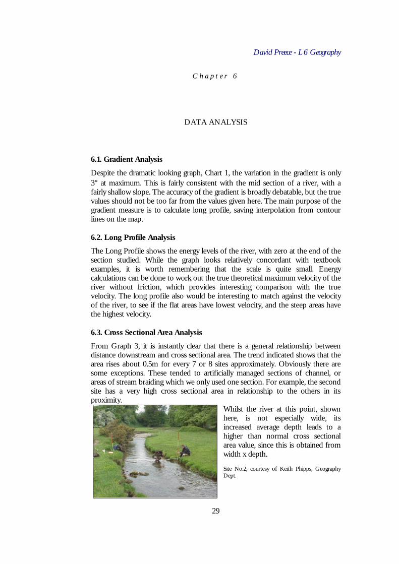
6.3. Cross Sectional Area Analysis From Graph 3, it is instantly clear that there is a general relationship between distance downstream and cross sectional area. The trend indicated shows that the area rises about 0.5m for every 7 or 8 sites approximately. Obviously there are some exceptions. These tended to artificially managed sections of channel, or areas of stream braiding which we only used one section. For example, the second site has a very high cross sectional area in relationship to the others in its proximity.

Whilst the river at this point, shown here, is not especially wide, its increased average depth leads to a higher than normal cross sectional area value, since this is obtained from width x depth. Site No.2, courtesy of Keith Phipps, Geography Dept.


30

If all of the values above 1.5m were ignored, then the correlation would be remarkably good. As it stands the Spearman’s Rank Correlation Coefficient (SRCC henceforth!) value as calculated by Microsoft Excel is given as 0.587793. this indicates a positive correlation i.e. area increases as distance increases, and the value indicates a correlation of medium strength - there are some points close to the line, and others some distance away. The limitations of the graphing method of only using appropriate scale become apparent here. The variation between the line and the points are just 2 at maximum, whereas it appears a vast distance.

6.4. Velocity Analysis Graph 4 shows us that the general trend is a decreasing velocity with distance downstream. The points are scattered around the line of best fit in a relatively large variance. The SRCC of -0.51811 shows that the correlation is weak to moderate, and negative, which agrees with the graph. The are a number of points which are questionable, and are some way from the rest of the graph. An example of this would be at site 3, where the average velocity is some 0.94m/s. However, the temptation to ignore these points, and classify them merely as points of anomaly would be wrongly followed. The site in question was a very narrow and deep channel coming off a meander bend, and the water was funneled through this gap, resulting in a high velocity. Notice the artificial debris piled up on the inside of the meander to push the meander further to the right of this picture. Evidence of the power of this section can be observed in the amount of undercutting and collapse on the bank on the right. It is also notable that the maximum velocity on the whole river was recorded here in the centre of this section at 2.27m/s. There is also high velocity at the fourteenth site - which is just after the confluence at the Black Brook. This seems more inexplicable, and after looking at the photographs, it would seem difficult to ascertain why the velocity was so high. The gradual reduction in velocity over the section of the river has been ascribed to the presence of the artificial management, in particular, the weirs. The proximity of weirs a short distance from the end of the sample section will no doubt reduce the velocity upstream, much as a river will slow upon entering still water, because of the inertial dissipation of kinetic energy. This explains the reduction of velocity over the studied section.


31

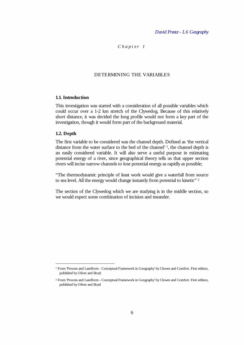
6.5. Discharge Analysis Like the velocity, Graph 5, the variation of discharge shows a downward trend with an increase in distance downstream. It appears to have a weak correlation, but the difference of axis scales makes it difficult to compare directly with velocity, thus Spearman’s Rank is used. An SRCC value of -0.43521 shows us that the correlation is less than the correlation of velocity. It is a poor to weak correlation, and has an overall downward trend. This proves that the original hypothesis that discharge would increase with distance downstream is wrong. This undoubtedly has been influenced by the decrease in velocity. The influence of the artificial management using the weirs has modified the result of this section. The ‘backlog’ effect of the weirs can be judged to have influenced the last four sections, 21-24, only. However, the graph’s shape is not the only factor to have affected the downwards trend of the graph. The artificial narrowing of the channel at the start of the section has boosted the velocity values for the start of the graph. Thus, if we plot the graph of velocity and discharge again, we should see a general increase in both, which would correlate with accepted theory. Regrettably, the values give a trendline which is

almost parallel to the x-axis. The correlation for this graph has been given as 0.001285. the proximity of this value to zero shows just how little correlation there appears to be. However,

since the overall trend of the cross section area was an increasing one, it would seem to indicate that the graph of discharge would concur with accepted theory. However, it seems that the correlation still does not match the theoretical ideal relationship which we would expect from a river. This is acceptable considering the limitations of the collection of the data, which will be discussed in the evaluation chapter.

Downstream Flow Variables Ignoring those afftected by artificial management.

0

0.2

0.4

0.6

0.8

5 6 7 8 9 10 11 12 13 14 15 16 17 18 19 20

Site Number

Vel

oci

ty (

m/s

)

Downstream flow variables (Discharge) ignoring the effects of artificial management

0

0.1

0.2

0.3

0.4

0.5

0.6

5 6 7 8 9 10 11 12 13 14 15 16 17 18 19 20Site Number

Dis

char

ge

(cu

mec

s)


32

6.6. Analysis of the testing of Leopold and Maddocks’ flow variables In both the test cases, the relationships between Leopold and Maddocks predicted variations and the variations which we recorded are somewhat different. In the case of Graph 6, the relationship between cross section and discharge produced a graph which had a correlation of -0.40666. The weak to moderate correlation does not indicate such a clear relationship as Leopold and Maddocks’ would suggest. In addition, the negative relationship does not fit with Leopold and Maddocks’ work, and this difference can clearly be seen on the graph, not only in the values, but also in the general shape of the curve. In the case of Graph 7, the relationship between velocity and discharge produced a graph which had a correlation between real and predicted of 0.766512. This is by far the strongest correlation we have seen in all of the results, and reflects a similar direction of the relationship, i.e. both increase with discharge. The difference between the rate of increase in our work and that of Leopold and Maddocks is noticeable. Our velocity increases far more rapidly than discharge, but is at a lower value than that predicted by the relationship suggested by Leopold and Maddocks. It would seem relevant to point out, however, how the data for discharge did not conform to our expectations, and thus we must treat all comparisons to discharge with some degree of suspicion. I think that the comparison of the results to those relationships predicted by Leopold and Maddocks is a useful check on how the river conforms to expectations generally. It is obvious from the considered analysis of all of the data that the river does not conform to expectations. The principal influence on the discharge of the river has been the independence of the velocity. This has been considerably altered by the artificial anthropogenic management of the river, presumably by the landowners, the National Trust. Whilst the access guaranteed by the Trust is a useful asset in choosing a location for the study, the aspects of river management which have altered the results of the study may make the choice of location a poor one in retrospect. However, we cannot realistically expect the studied section, at just under 2 km in length, to accurately compare to an detailed study which encompassed many rivers of a much greater length than we are dealing with. This would be even less likely with the impact of human management to the extent which we have seen on the short section we studied.


33

C h a p t e r 7

EVALUATION OF RESULTS, TECHNIQUE AND LOCATION OF THE STUDY

It is obvious that such a study as this, with such a constraint on time, would be flawed. In this chapter, an attempt will be made to identify the main problems, and ideas for their resolution. The first problem was the lack of access and transport and time, all of which meant that we could not survey the entire river, but only a 2 km section. This naturally reduced the accuracy of the study. We cannot generalise about rivers based on a sample of river which is unrepresentative of the whole river due to its heavy human management. Within the allotted time, there was no feasible way to survey the entire river, but this would really improve our accuracy, and help us to make more general conclusions from the data that would be collected. The amount of resources available would determine the sample intervals which could be worked on. For example, if we had few resources, we could use a kilometre interval to obtain about cross section from the entire river. Obviously, the smaller sample interval would give more samples, and a more accurate result. Using a 50m sample interval along the entire river would give a very accurate result, but processing 450 results would be quite difficult and time consuming. The second problem was the location of the study. Whilst it was ideally placed for access, and for its varied nature, it was only when the results were evaluated that it was realised to what extent the channel was managed. This management influenced the results in several ways, both increasing and reducing the velocity at various points in the channel, as discussed previously. The impact of this management has, I believe, altered the results so much so that it does not concur with accepted theoretical rationale. Had the weir not affected the velocity downstream, and it had in fact increased at the rate previously seen then perhaps all the results would have been different. I do not see a way to reduce the impact of the management schemes on the study. The only alternative is to choose an unmanaged river, if there is such a thing. The extent of the management is shown overleaf. The weirs have fulfilled their designed purpose - to regulate the flow of the river, as well as acting as a speed and sediment trap. There is evidence of


35

alluvial deposits, suggesting that the river may still flood, and this is why the river is controlled in the way that it is. In terms of the methods and accuracy of the techniques used, then I believe them to be sufficiently accurate to serve the purposes of the study. With the software available, then the measurements taken are quite sufficient to produce a cross section with all the data on it. I would not alter the techniques used, and it is worth noting that this is standard procedure in all textbooks, and even at Oxford. There are no problems with the techniques. The results are presented in format which is entirely applicable to the data concerned. There is no problem with the presentation, manipulation and processing of the data due to the software used. I used Microsoft Excel for the presentation of the data. This allowed rapid manipulation, and the ability to copy chunks of data from sheets so I did not have to re-type lists over and over again. It also allowed me to alter scales and types of graph, and insert computer placed trendlines, which were far more accurate than I could have drawn. It also allowed rapid statistical calculations of Spearman’s Rank Correlation Coefficient, which saved doing it all laboriously by hand. This was most beneficial, and allowed me to proceed with the analysis, rather than spending time on this. In terms of presenting the graphs, I have used scattergraphs throughout. They allow accurate plotting of points on a scale, and also allow points to be plotted on a non-standard scale, e.g. against discharge. This was very useful to compare data against predicted relationships without resorting to complex calculations. In terms of extending the investigation further, the extension of the surveyed area is the most obvious choice, for reasons explained earlier. An interesting point of note is the sudden loss of discharge after an increase following the confluence with the Black Brook. The area is known for its history of subsidence, indeed a subsidence lake was found in the centre of the flood plain at GR. 330 487. An investigation in to the underlying geology of the area would be an stimulating one. It would also be fascinating to investigate the water exchange between this lake and the river, in terms of seasonal water table variation. It would also be intriguing to investigate the extent to which the post confluential river is the sum of the discharges of the Clywedog and the Black Brook. To do this, an analysis of the discharges of both channels would need to be carried out. This could be related to Strahler’s stream order theory. A brief return to Edwards work shows us that over a longer length of the same river, the model is more concurrent with reality. Thus we know that the work can be done in accordance with what it should be, if sufficient data is considered.


36

C h a p t e r 8

LIST OF SOURCES

Clowes and Comfort; ‘Process and Landform - Conceptual Framework in Geography’. Oliver and Boyd, 1st edition. Hilton, Keith; ‘Process and Pattern in Physical Geography’. University Tutorial, 3rd edition. Lenon and Cleves; ‘Fieldwork Techniques and Projects in Geography’. Harper Educational, 1st edition. Mc Cullagh, Patrick; ‘Modern Concepts in Geomorphology’. Oxford University Press, 2nd edition. Waugh, David; ‘Geography - An Integrated Approach’. 3rd edition, published by Nelson

David Preece - L6 Geography - · PDF fileDavid Preece - L6 Geography 1 AN INVESTIGATION IN TO...

Documents

Transcript of David Preece - L6 Geography - · PDF fileDavid Preece - L6 Geography 1 AN INVESTIGATION IN TO...