David H. Brainard - University of...
56
COLORIMETRY David H. Brainard Department of Psychology University of Pennsylvania Philadelphia, Pennsylvania Andrew Stockman Department of Visual Neuroscience UCL Institute of Ophthalmology London, United Kingdom 10.1 GLOSSARY Chromaticity coordinates. Tristimulus values normalized to sum to unity. CIE. Commission Internationale de l’Éclairage or International Commission on Illumination. Organization that develops standards for color and lighting. Color-matching functions (CMFs). Tristimulus values of the equal-energy spectrum locus. Color space transformation matrix. Multiply a vector of tristimulus values for one color space by such a matrix to obtain tristimulus values in another color space. Cone coordinates. Tristimulus values of a light with respect to the cone fundamentals. Cone fundamentals. Estimates of the cone spectral sensitivities at the cornea. Equivalently, the CMFs that would result if primaries that uniquely stimulated the three cones could be and were used. Linear model. Set of spectral functions that may be scaled and added to approximate other spec- tral functions. For example, the spectral power distributions of three monitor primaries are a linear model for the set of lights that can be emitted by the monitor. Metamers. Two physically different lights that match in appearance to an observer. Photopic luminosity function. Measure of luminous efficiency as a function of wavelength under photopic (i.e., rod-free) conditions. Primary lights. Three independent lights (real or imaginary) to whose scaled mixture a test light is matched (actually or hypothetically). They must be independent in the sense that no combination of any two can match the third. Standard observer. The standard observer is the hypothetical individual whose color-matching behavior is represented by a particular set of CMFs. Tristimulus values. The tristimulus values of a light are the intensities of the three primary lights required to match it. Visual angle. The angle subtended by an object in the external field at the effective optical center of the eye. Colorimetric data are typically specified for centrally fixated 2° or 10° fields of view. 10.1 10 Bass_v3ch10_p001-056.indd 10.1 Bass_v3ch10_p001-056.indd 10.1 8/21/09 12:49:46 PM 8/21/09 12:49:46 PM
Transcript of David H. Brainard - University of...

COLORIMETRY
David H. BrainardDepartment of PsychologyUniversity of PennsylvaniaPhiladelphia, Pennsylvania
Andrew StockmanDepartment of Visual NeuroscienceUCL Institute of OphthalmologyLondon, United Kingdom
10.1 GLOSSARY
Chromaticity coordinates. Tristimulus values normalized to sum to unity.
CIE. Commission Internationale de l’Éclairage or International Commission on Illumination. Organization that develops standards for color and lighting.
Color-matching functions (CMFs). Tristimulus values of the equal-energy spectrum locus.
Color space transformation matrix. Multiply a vector of tristimulus values for one color space by such a matrix to obtain tristimulus values in another color space.
Cone coordinates. Tristimulus values of a light with respect to the cone fundamentals.
Cone fundamentals. Estimates of the cone spectral sensitivities at the cornea. Equivalently, the CMFs that would result if primaries that uniquely stimulated the three cones could be and were used.
Linear model. Set of spectral functions that may be scaled and added to approximate other spec-tral functions. For example, the spectral power distributions of three monitor primaries are a linear model for the set of lights that can be emitted by the monitor.
Metamers. Two physically different lights that match in appearance to an observer.
Photopic luminosity function. Measure of luminous effi ciency as a function of wavelength under photopic (i.e., rod-free) conditions.
Primary lights. Three independent lights (real or imaginary) to whose scaled mixture a test light is matched (actually or hypothetically). They must be independent in the sense that no combination of any two can match the third.
Standard observer. The standard observer is the hypothetical individual whose color-matching behavior is represented by a particular set of CMFs.
Tristimulus values. The tristimulus values of a light are the intensities of the three primary lights required to match it.
Visual angle. The angle subtended by an object in the external fi eld at the effective optical center of the eye. Colorimetric data are typically specifi ed for centrally fi xated 2° or 10° fi elds of view.
10.1
10
Bass_v3ch10_p001-056.indd 10.1Bass_v3ch10_p001-056.indd 10.1 8/21/09 12:49:46 PM8/21/09 12:49:46 PM

10.2 VISION AND VISION OPTICS
10.2 INTRODUCTION
Scope
The goal of colorimetry is to incorporate properties of the human color vision system into the mea-surement and numerical specification of visible light. Thanks in part to the inherent simplicity of the initial stages of visual coding, this branch of color science has been quite successful. We now have effective quantitative representations that predict when two lights will appear identical to a human observer and a good understanding of how these matches are related to the spectral sensitiv-ities of the underlying cone photoreceptors. Although colorimetric representations do not directly predict color sensation,1–3 they do provide the foundation for the scientific study of color appear-ance. Moreover, colorimetry can be applied successfully in practical applications. Foremost among these is perhaps color reproduction.4–6
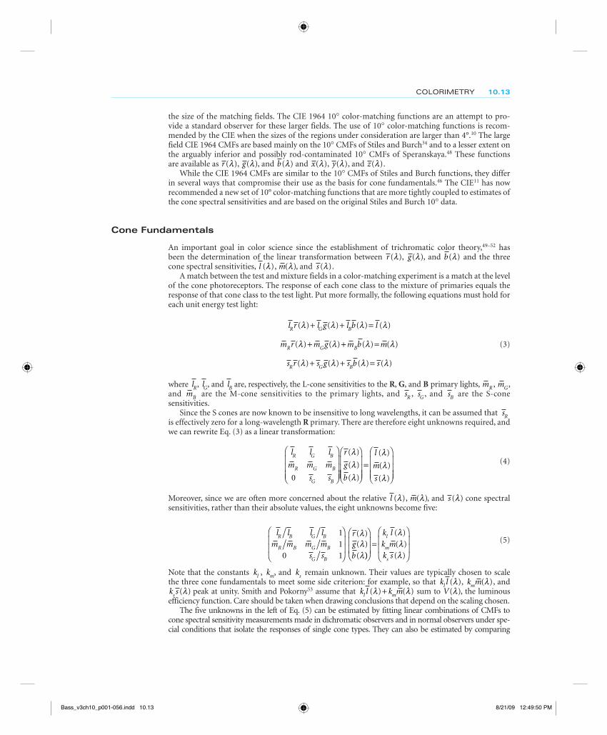
As an illustrative example, Fig. 1 shows an image processing chain. Light from an illuminant reflects from a collection of surfaces. This light is recorded by a color camera and stored in digital form. The digital image is processed by a computer and rendered on a color monitor. The reproduced image is viewed by a human observer. The goal of the image processing is to render an image with the same color appearance at each image location as the original. Although exact reproduction is not always possible with this type of system, the concepts and formulas of colorimetry do provide a reasonable solution.4,7 To develop this solution, we will need to consider how to represent the spectral properties of light, the relation between these properties and color camera responses, the representation of the restricted set of lights that may be produced with a color monitor, and the way in which the human visual system encodes the spectral properties of light. We will treat each of these topics in this chapter, with particular emphasis on the role played by the human visual system.
Reference Sources
A number of excellent references are available that provide detailed treatments of colorimetry and its applications. Wyszecki and Stiles’ comprehensive book8 is an authoritative reference and
Humanobserver
Illuminant
Surface
Color camera
Monitor
FIGURE 1 A typical image processing chain. Light reflects from a surface or collection of surfaces. This light is recorded by a color camera and stored in digital form. The digital image is processed by a computer and rendered on a color monitor. The reproduced image is viewed by a human observer.
Bass_v3ch10_p001-056.indd 10.2Bass_v3ch10_p001-056.indd 10.2 8/21/09 12:49:47 PM8/21/09 12:49:47 PM
COLORIMETRY 10.3
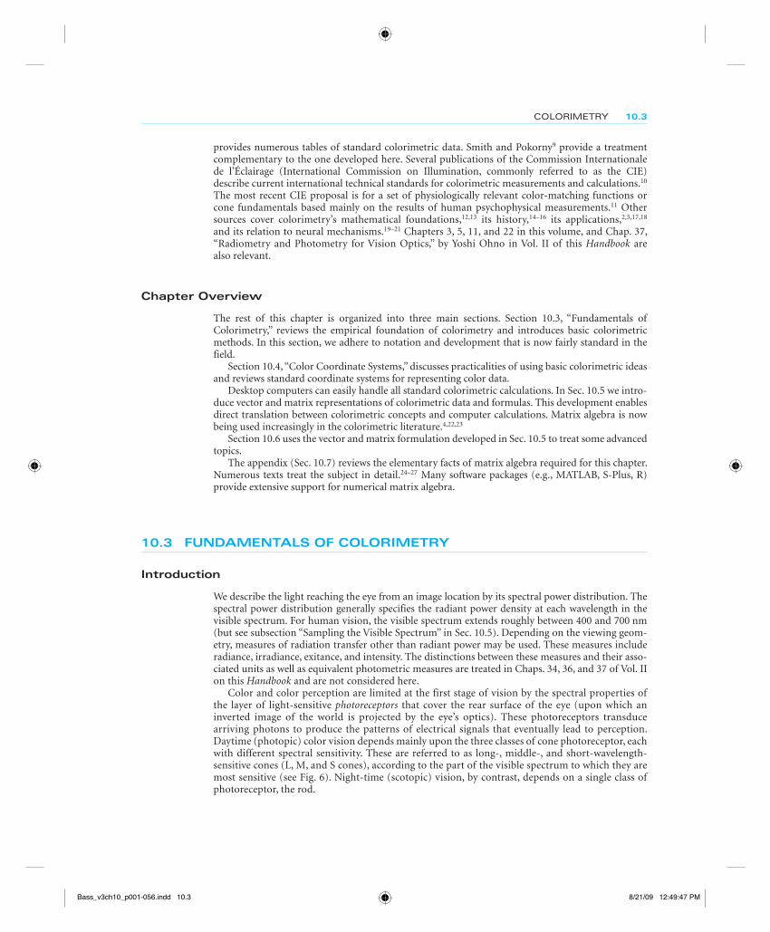
provides numerous tables of standard colorimetric data. Smith and Pokorny9 provide a treatment complementary to the one developed here. Several publications of the Commission Internationale de l’Éclairage (International Commission on Illumination, commonly referred to as the CIE) describe current international technical standards for colorimetric measurements and calculations.10 The most recent CIE proposal is for a set of physiologically relevant color-matching functions or cone fundamentals based mainly on the results of human psychophysical measurements.11 Other sources cover colorimetry’s mathematical foundations,12,13 its history,14–16 its applications,2,5,17,18 and its relation to neural mechanisms.19–21 Chapters 3, 5, 11, and 22 in this volume, and Chap. 37, “Radiometry and Photometry for Vision Optics,” by Yoshi Ohno in Vol. II of this Handbook are also relevant.
Chapter Overview
The rest of this chapter is organized into three main sections. Section 10.3, “Fundamentals of Colorimetry,” reviews the empirical foundation of colorimetry and introduces basic colorimetric methods. In this section, we adhere to notation and development that is now fairly standard in the field.
Section 10.4, “Color Coordinate Systems,” discusses practicalities of using basic colorimetric ideas and reviews standard coordinate systems for representing color data.
Desktop computers can easily handle all standard colorimetric calculations. In Sec. 10.5 we intro-duce vector and matrix representations of colorimetric data and formulas. This development enables direct translation between colorimetric concepts and computer calculations. Matrix algebra is now being used increasingly in the colorimetric literature.4,22,23
Section 10.6 uses the vector and matrix formulation developed in Sec. 10.5 to treat some advanced topics.
The appendix (Sec. 10.7) reviews the elementary facts of matrix algebra required for this chapter. Numerous texts treat the subject in detail.24–27 Many software packages (e.g., MATLAB, S-Plus, R) provide extensive support for numerical matrix algebra.
10.3 FUNDAMENTALS OF COLORIMETRY
Introduction
We describe the light reaching the eye from an image location by its spectral power distribution. The spectral power distribution generally specifies the radiant power density at each wavelength in the visible spectrum. For human vision, the visible spectrum extends roughly between 400 and 700 nm (but see subsection “Sampling the Visible Spectrum” in Sec. 10.5). Depending on the viewing geom-etry, measures of radiation transfer other than radiant power may be used. These measures include radiance, irradiance, exitance, and intensity. The distinctions between these measures and their asso-ciated units as well as equivalent photometric measures are treated in Chaps. 34, 36, and 37 of Vol. II on this Handbook and are not considered here.
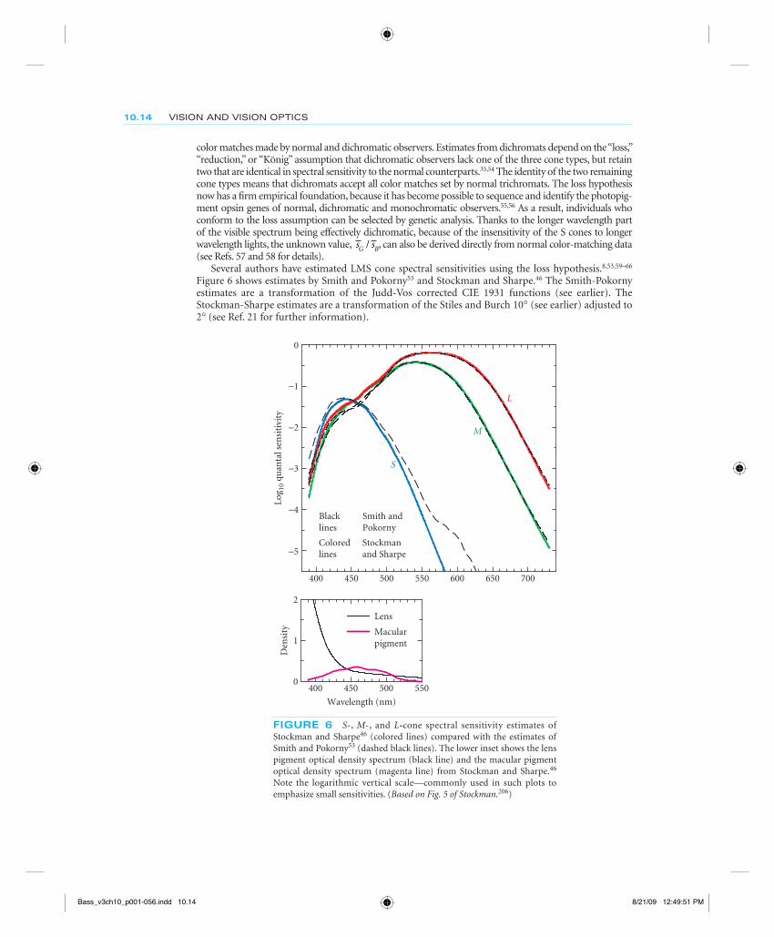
Color and color perception are limited at the first stage of vision by the spectral properties of the layer of light-sensitive photoreceptors that cover the rear surface of the eye (upon which an inverted image of the world is projected by the eye’s optics). These photoreceptors transduce arriving photons to produce the patterns of electrical signals that eventually lead to perception. Daytime (photopic) color vision depends mainly upon the three classes of cone photoreceptor, each with different spectral sensitivity. These are referred to as long-, middle-, and short-wavelength-sensitive cones (L, M, and S cones), according to the part of the visible spectrum to which they are most sensitive (see Fig. 6). Night-time (scotopic) vision, by contrast, depends on a single class of photoreceptor, the rod.
Bass_v3ch10_p001-056.indd 10.3Bass_v3ch10_p001-056.indd 10.3 8/21/09 12:49:47 PM8/21/09 12:49:47 PM
10.4 VISION AND VISION OPTICS
Conventional Colorimetric Terms and Notation
Table 1 provides a glossary of conventional colorimetric terms and notation. We adhere to these conventions in our initial development, in this section and in Sec.10.4. See also Table 3.1 of Ref. 28, and compare with the matrix algebra glossary in Table 2.
Trichromacy and Univariance
Normal human vision is trichromatic. With some important provisos (see subsection “Conditions for Trichomatic Color Matching” in Sec. 10.3), observers can match a test light of any spectral com-position to an appropriately adjusted mixture of just three other lights. Consequently, colors can be defined by three variables: the intensities of the three primary lights with which they match. These are called tristimulus values.
The range of colors that can be produced by the additive combination of three lights is simulated in Fig. 2. Overlapping red, green, and blue lights produce regions that appear cyan, purple, yellow, and white. Other, intermediate, colors can be produced by varying the relative intensities of the three lights.
Human vision is trichromatic because there are only three classes of cone photoreceptor in the eye, each of which responds univariantly to the rate of photon absorption.29,30 Univariance refers to the fact that the effect of a photon, once absorbed, is independent of wavelength. What varies with wavelength is the probability that a photon is in fact absorbed, and this variation is described by the photoreceptor’s spectral sensitivity. Photoreceptors are, in effect, sophisticated photon counters the outputs of which vary according to the rate of absorbed photons. Changes in the absorption rate can result from a change in photon wavelength or from a change in the number of incident photons. This confound means that individual photoreceptors are effectively color blind. Normal observers are able to see color by comparing the outputs of the three, individually color-blind, cone types.
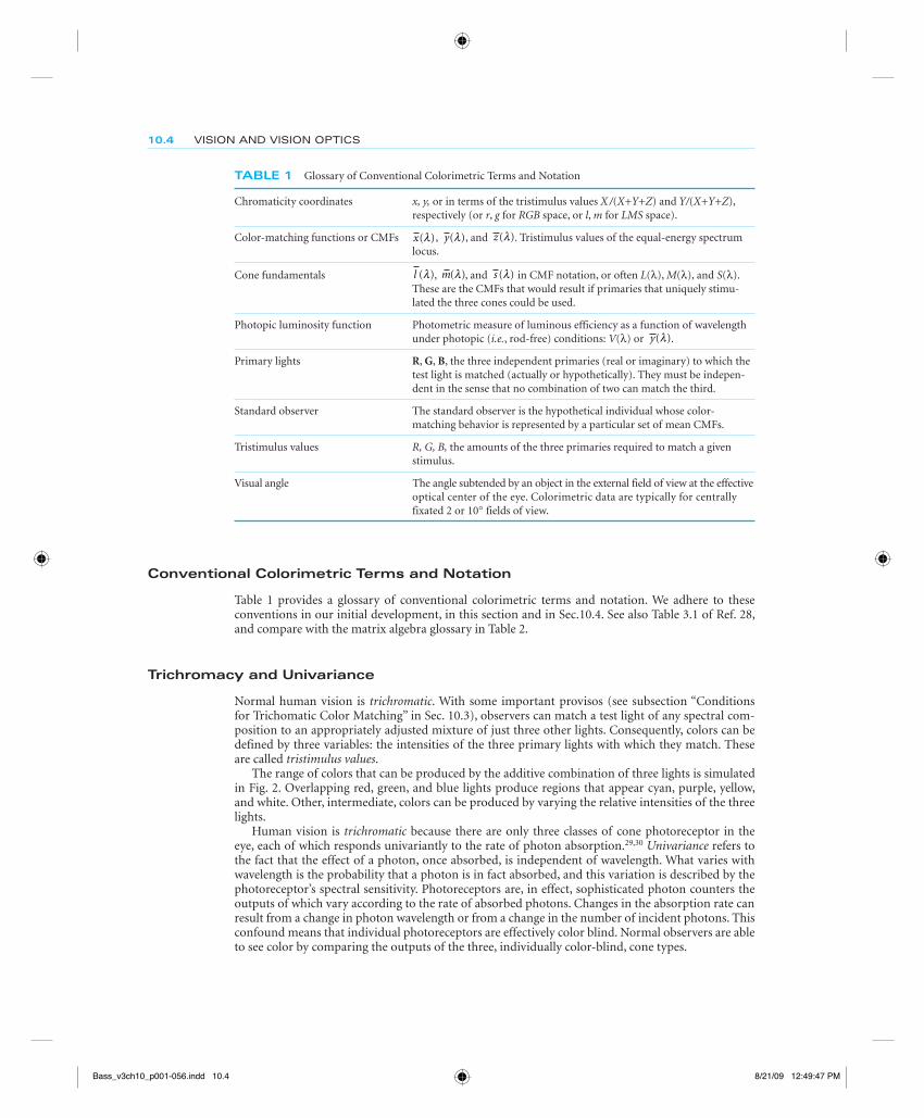
TABLE 1 Glossary of Conventional Colorimetric Terms and Notation
Chromaticity coordinates x, y, or in terms of the tristimulus values X /(X+Y+Z) and Y/(X+Y+Z), respectively (or r, g for RGB space, or l, m for LMS space).
Color-matching functions or CMFs x( )λ , y( )λ , and z( )λ . Tristimulus values of the equal-energy spectrum locus.
Cone fundamentals l ( )λ , m( )λ , and s ( )λ in CMF notation, or often L(λ), M(λ), and S(λ). These are the CMFs that would result if primaries that uniquely stimu-lated the three cones could be used.
Photopic luminosity function Photometric measure of luminous efficiency as a function of wavelength under photopic (i.e., rod-free) conditions: V(λ) or y( )λ .
Primary lights R, G, B, the three independent primaries (real or imaginary) to which the test light is matched (actually or hypothetically). They must be indepen-dent in the sense that no combination of two can match the third.
Standard observer The standard observer is the hypothetical individual whose color-matching behavior is represented by a particular set of mean CMFs.
Tristimulus values R, G, B, the amounts of the three primaries required to match a given stimulus.
Visual angle The angle subtended by an object in the external field of view at the effective optical center of the eye. Colorimetric data are typically for centrally fixated 2 or 10° fields of view.
Bass_v3ch10_p001-056.indd 10.4Bass_v3ch10_p001-056.indd 10.4 8/21/09 12:49:47 PM8/21/09 12:49:47 PM

TABLE 2 Glossary of Notation Used in Matrix Algebra Development
Link to Conventional Notation
l Wavelength
Nl Number of wavelength samples
b Spectral power distribution; basis vector
B Linear model basis vectors
a Linear model weights
Nb Linear model dimension
p Primary spectral power distribution
P Linear model for primaries
t Tristimulus coordinates XYZ
⎡
⎣
⎢⎢
⎤
⎦
⎥⎥
T Color-matching functions • • • • • •• • • • • •• • •
x
y
zz • • •
⎡
⎣
⎢⎢⎢
⎤
⎦
⎥⎥⎥
(x, y , and z are rows of T)
r Cone (or sensor) coordinates LMS
⎡
⎣
⎢⎢
⎤
⎦
⎥⎥
R Cone (or sensor) sensitivities • • • • • •• • • • • •• •
l
m
• • • •
⎡
⎣
⎢⎢⎢
⎤
⎦
⎥⎥⎥s
( l , m, and s are rows of R )
v Luminance Y[ ]
V Luminous efficiency function • • • • • •⎡⎣ ⎤⎦Vλ (Vl is the single row of vector v)
M Color space transformation matrix
10.5
FIGURE 2 Additive color mixing. Simulated overlap of projected red, green, and blue lights. The additive combination of red and green is seen as yellow, red and blue as purple, green and blue as cyan, and red, green, and blue as white.
Bass_v3ch10_p001-056.indd 10.5Bass_v3ch10_p001-056.indd 10.5 8/21/09 12:49:47 PM8/21/09 12:49:47 PM
10.6 VISION AND VISION OPTICS
Color Matching
Trichromacy, together with other critical properties of color matching described in subsection “Critical Properties of Color Matching” in Sec. 10.3 mean that the color-matching behavior of an individual can be characterized as the intensities of three independent primary lights that are required to match a series of monochromatic spectral lights spanning the visible spectrum. Two experimental methods have been used to measure color matches: the maximum saturation method and Maxwell’s method. Most standard color-matching functions have been obtained using the max-imum saturation method, though it is arguably inferior.
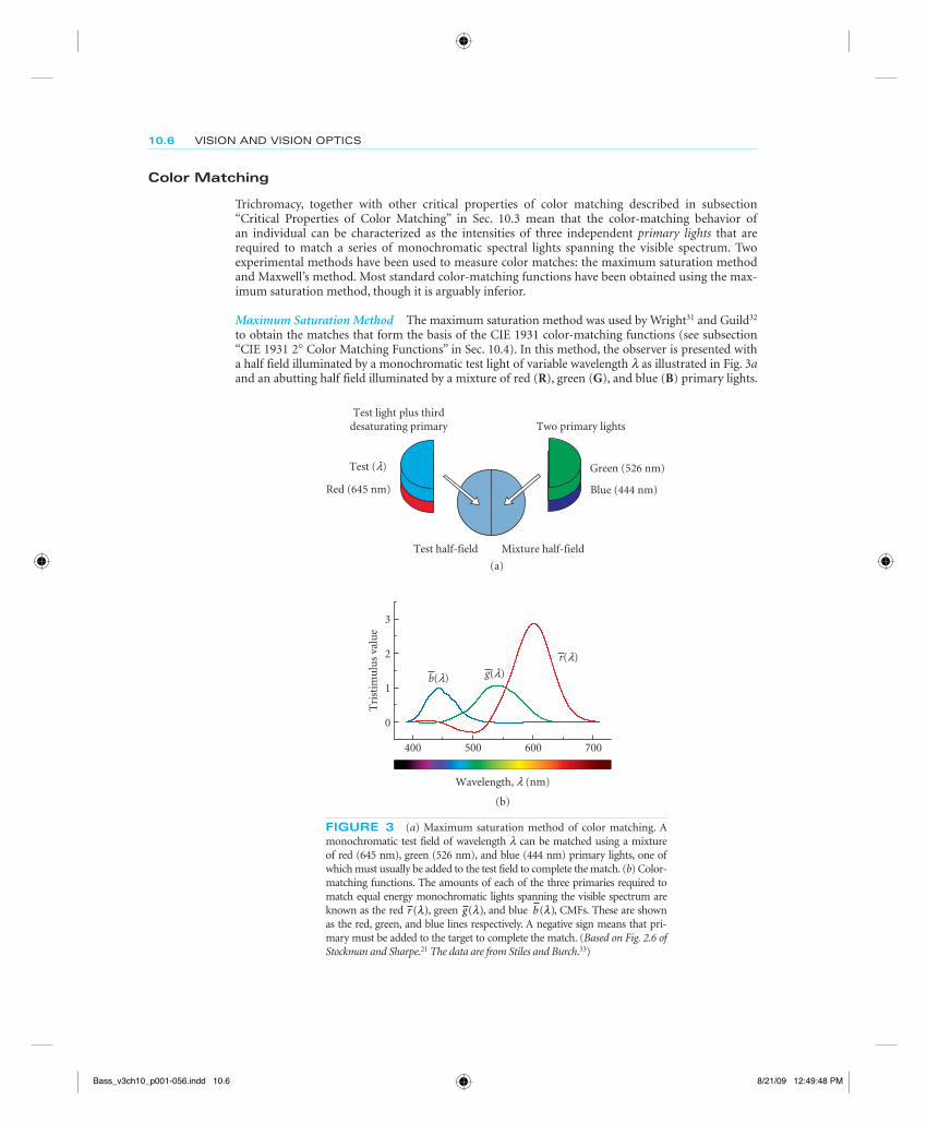
Maximum Saturation Method The maximum saturation method was used by Wright31 and Guild32 to obtain the matches that form the basis of the CIE 1931 color-matching functions (see subsection “CIE 1931 2° Color Matching Functions” in Sec. 10.4). In this method, the observer is presented with a half field illuminated by a monochromatic test light of variable wavelength l as illustrated in Fig. 3a and an abutting half field illuminated by a mixture of red (R), green (G), and blue (B) primary lights.
Wavelength, l (nm)
400 500 600 700
Tri
stim
ulu
s va
lue
0
1
2
3
b(l) g(l)
r(l)
Mixture half-fieldTest half-field
Red (645 nm)
Green (526 nm)
Blue (444 nm)
Two primary lights
Test (l)
Test light plus thirddesaturating primary
(a)
(b)
FIGURE 3 (a) Maximum saturation method of color matching. A monochromatic test field of wavelength l can be matched using a mixture of red (645 nm), green (526 nm), and blue (444 nm) primary lights, one of which must usually be added to the test field to complete the match. (b) Color-matching functions. The amounts of each of the three primaries required to match equal energy monochromatic lights spanning the visible spectrum are known as the red r ( )λ , green g( )λ , and blue b( )λ , CMFs. These are shown as the red, green, and blue lines respectively. A negative sign means that pri-mary must be added to the target to complete the match. (Based on Fig. 2.6 of Stockman and Sharpe.21 The data are from Stiles and Burch.33)
Bass_v3ch10_p001-056.indd 10.6Bass_v3ch10_p001-056.indd 10.6 8/21/09 12:49:48 PM8/21/09 12:49:48 PM

COLORIMETRY 10.7
(Note that in this section of the chapter, bold uppercase symbols denote primary lights, not matrices.) Often the primary lights are chosen to be monochromatic, although this is not necessary. For each test wavelength l, the observer adjusts the intensities and arrangement of the three primary lights to make a match between the half field containing the test light and the adjacent half field. Generally, one of the primary lights is admixed with the test, while the other two are mixed together in the adjacent half field. Figure 3b shows the mean r ( )λ , g( )λ , and b( )λ color-matching functions (hereafter abbrevi-ated as CMFs) obtained by Stiles and Burch33 for primary lights of 645, 526, and 444 nm. Notice that one of the CMFs is usually negative. There is no “negative light.” Negative values mean that the primary in question has been added to the test light in order to make a match. Matches using real primaries result in negative values because the primaries do not uniquely stimulate single cone pho-toreceptors, the spectral sensitivities of which overlap throughout the visible spectrum (see Fig. 6). Although color-matching functions are generally plotted as functions of wavelength, it is helpful to keep in mind that they represent matches, not light spectral power distributions.
The maximum saturation match between Eλ , a monochromatic constituent of the equal unit energy stimulus of wavelength l, and the three primary lights (R, , andG B) is denoted by
E R G Bλ λ λ λ~ ( ) ( ) ( )r g b+ + (1)
where r ( )λ , g( )λ , and b( )λ are the three CMFs, and where negative CMF values indicate that the corresponding primary was mixed with the test to make the perceptual match. CMFs are usually defined for a stimulus, E, which has equal unit energy throughout the spectrum. However, in prac-tice the spectral power of the test light used in most matching experiments is varied with wave-length. In particular, longer-wavelength test lights are typically chosen to be intense enough to satu-rate the rods so that rods do not participate in the matches (see, e.g., Ref. 34). CMFs and the spectral power distributions of lights are always measured and tabulated as discrete functions of wavelength, typically defined in steps of 1, 5, or 10 nm.
We use the symbol ~ in Eq. (1) to indicate that two lights are a perceptual match. Perceptual matches are to be carefully distinguished from physical matches, which are denoted by the = symbol. Of course, when two lights are a physical match, they must also be a perceptual match. Two lights that are a percep-tual match but not a physical match are referred to as metameric color stimuli or metamers. The term metamerism is often used to refer to the fact that two physically different lights can appear identical.
The color-matching functions are defined for equal energy monochromatic test lights. More generally any test light, whether monochromatic or not, may be matched in the color-matching exper-iment. As noted above, we refer to the primary weights R, G, and B required to match any light as its tristimulus values. As with CMFs, tristimulus values may be negative, indicating that the correspond-ing primary is mixed with the test to make the match. Once the matching primaries are specified, the tristimulus values of a light provide a complete description of its effect on the human cone-mediated visual system, subject to the caveats discussed below. In addition, knowledge of the color-matchingfunctions is sufficient to compute the tristimulus values of any light (see subsection “Tristimulus Values for Arbitrary lights” in Sec. 10.3).
Conditions for Trichromatic Color Matching There are a number of qualifications to the empirical generalization that it is possible for observers to match any test light by adjusting the intensities of just three primaries. Some of these qualifications have to do with ancillary restrictions on the exper-imental conditions (e.g., the size of the bipartite field and the overall intensity of the test and match-ing lights). The other qualifications have to do with the choice of primaries and certain conventions about the matching procedure. First the primaries must be chosen so that it is not possible to match any one of them with a weighted superposition of the other two. Second, the observer sometimes wishes to increase the intensity of one or more of the primaries above its maximum value. In this case, we must allow him to scale the intensity of the test light down. We follow the convention of saying that the match was possible and scale up the reported primary weights by the same factor. Third, as discussed in more detail above, the observer sometimes wishes to decrease the intensity of one or more of the primaries below zero. This is always the case when the test light is a spectral light unless its wavelength is equivalent to one of the primaries. In this case, we must allow the observer
Bass_v3ch10_p001-056.indd 10.7Bass_v3ch10_p001-056.indd 10.7 8/21/09 12:49:48 PM8/21/09 12:49:48 PM
10.8 VISION AND VISION OPTICS
to superimpose each such primary on the test light rather than on the other primaries. We follow the convention of saying that the match was possible but report with negative sign the intensity of each transposed primary.
With these qualifications, matching with three primaries is always possible for small fields. For larger fields, spatial inhomogeneities may make it impossible to produce a match simultaneously across the entire field (see subsections “Specifity of CMFs” and “Tristimulus Values for Arbitrary Lights” in Sec. 10.3).
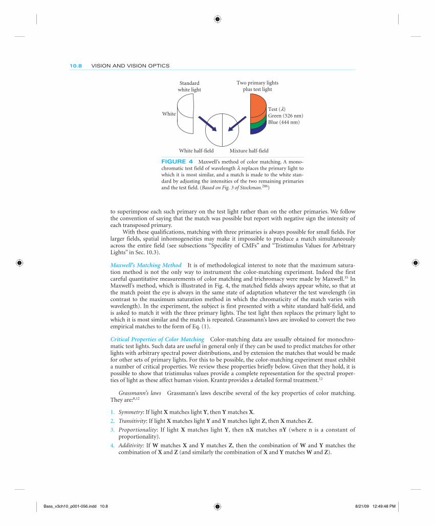
Maxwell’s Matching Method It is of methodological interest to note that the maximum satura-tion method is not the only way to instrument the color-matching experiment. Indeed the first careful quantitative measure ments of color matching and trichromacy were made by Maxwell.35 In Maxwell’s method, which is illustrated in Fig. 4, the matched fields always appear white, so that at the match point the eye is always in the same state of adaptation whatever the test wavelength (in contrast to the maximum saturation method in which the chromaticity of the match varies with wavelength). In the experiment, the subject is first presented with a white standard half-field, and is asked to match it with the three primary lights. The test light then replaces the primary light to which it is most similar and the match is repeated. Grassmann’s laws are invoked to convert the two empirical matches to the form of Eq. (1).
Critical Properties of Color Matching Color-matching data are usually obtained for monochro-matic test lights. Such data are useful in general only if they can be used to predict matches for other lights with arbitrary spectral power distributions, and by extension the matches that would be made for other sets of primary lights. For this to be possible, the color-matching experiment must exhibit a number of critical properties. We review these properties briefly below. Given that they hold, it is possible to show that tristimulus values provide a complete representation for the spectral proper-ties of light as these affect human vision. Krantz provides a detailed formal treatment.12
Grassmann’s laws Grassmann’s laws describe several of the key properties of color matching. They are:8,12
1. Symmetry: If light X matches light Y, then Y matches X.
2. Transitivity: If light X matches light Y and Y matches light Z, then X matches Z.
3. Proportionality: If light X matches light Y, then nX matches nY (where n is a constant of proportionality).
4. Additivity: If W matches X and Y matches Z, then the combination of W and Y matches the combination of X and Z (and similarly the combination of X and Y matches W and Z).
Mixture half-fieldWhite half-field
Test (l)Green (526 nm)Blue (444 nm)
Standardwhite light
Two primary lightsplus test light
White
FIGURE 4 Maxwell’s method of color matching. A mono-chromatic test field of wavelength l replaces the primary light to which it is most similar, and a match is made to the white stan-dard by adjusting the intensities of the two remaining primaries and the test field. (Based on Fig. 3 of Stockman.206)
Bass_v3ch10_p001-056.indd 10.8Bass_v3ch10_p001-056.indd 10.8 8/21/09 12:49:48 PM8/21/09 12:49:48 PM
COLORIMETRY 10.9
These laws have been tested extensively and hold well.8,19 To a first approximation, color matching can be considered to be linear and additive.12,36
Uniqueness of color matches The tristimulus values of a light should be unique. This is equiva-lent to the requirement that only one weighted combination of the apparatus primaries produces a match to any given test light. The uniqueness of color matches ensures that tristimulus values are well-defined. In conjunction with transitivity, uniqueness also guarantees that two lights that match each other will have identical tristimulus values. It is generally accepted that, apart from variability, trichromatic color matches are unique for color normal observers.
Persistence of color matches The above properties concern color matching under a single set of viewing conditions. By viewing conditions, we refer to the properties of the image surrounding the bipartite field and the sequence of images viewed by the observer before he made the match. An important property of color matching is that lights that match under one set of viewing conditions continue to match when the viewing conditions are changed. This property is referred to as the per-sistence or stability of color matches.8, 19 It holds to good approximation (but see subsection “Limits of Color Matching Data” in Sec. 10.4). The importance of the persistence law is that it allows a single set of tristimulus values to be used across viewing conditions.
Consistency across observers Finally, for the use of tristimulus values to have general validity, it is important that there should be agreement about matches across observers. For the majority of the population, there is good agreement about which lights match. We discuss individual differences in color matching in section “Limits of Color-Matching Data.”
Specificity of CMFs Color-matching data are specific to the conditions under which they were measured, and strictly to the individual observers in whom they were measured. By applying the data to other conditions and using them to predict other observer’s matches, some errors will inevi-tably be introduced.
An important consideration is the area of the retina within which the color matches were made. Standard color matching data (see section “Color-Matching Functions” in Sec. 10.4) have been obtained for centrally viewed fields with diameters of either 2° or 10° of visual angle. The visual angle refers to the angle subtended by an object in the external field at the effective optical center of the eye. The size of a circular matching field used in colorimetry is defined as the angular difference subtended at the eye between two diametrically opposite points on the circumference of the field. Thus, matches are defined according to the retinal size of the matching field not by its physical size. A 2° diameter field is known as a small field, whereas a 10° one as a large field. (One degree of visual angle is roughly equivalent to the width of the fingernail of the index finger held at arm’s length.) Color matches vary with retinal size and position because of changes in macular pigment den-sity and photopigment optical density with visual angle (see section “Limits of Color-Matching Data”).
Standardized CMFs are mean data that are also known as standard observer data, in the sense that they are assumed to represent the color-matching behavior of a hypothetical typical human observer. The color matches of individual observers, however, can vary substantially from the mean matches represented by standard observer CMFs. Individual differences in lens pigment density, macular pig-ment density, photopigment optical density, and in the photopigments themselves can all influence color matches (see section “Limits of Color-Matching Data”).
Tristimulus Values for Arbitrary Lights Given that additivity holds for color matches, the tristimu-lus values, R, G, and B for an arbitrarily complex spectral radiant power distribution P( )λ can be obtained from the r ( )λ , g( )λ , and b( )λ CMFs by:
R P r d= ∫ ( ) ( )λ λ λ , G P g d= ∫ ( ) ( )λ λ λ , and B P b d= ∫ ( ) ( )λ λ λ (2)
Since spectral power distributions and CMFs are usually discrete functions, the integration in Eq. (2) is usually replaced by a sum.
Bass_v3ch10_p001-056.indd 10.9Bass_v3ch10_p001-056.indd 10.9 8/21/09 12:49:49 PM8/21/09 12:49:49 PM
10.10 VISION AND VISION OPTICS
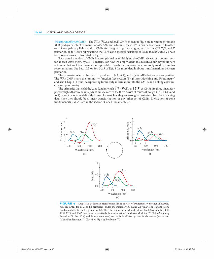
Transformability of CMFs The r ( )λ , g( )λ , and b( )λ CMFs shown in Fig. 3 are for monochromatic RGB (red-green-blue) primaries of 645, 526, and 444 nm. These CMFs can be transformed to other sets of real primary lights, and to CMFs for imaginary primary lights, such as the CIE X, Y, and Z primaries, or to CMFs representing the LMS cone spectral sensitivities (cone fundamentals). These transformations are illustrated in Fig. 5.
Each transformation of CMFs is accomplished by multiplying the CMFs, viewed as a column vec-tor at each wavelength, by a 3 × 3 matrix. For now we simply assert this result, as our key point here is to note that such transformation is possible to enable a discussion of commonly used tristimulus representations. See Sec. 10.5 or Sec. 3.2.5 of Ref. 8 for more details about transformations between primaries.
The primaries selected by the CIE produced x( )λ , y( )λ , and z( )λ CMFs that are always positive. The y( )λ CMF is also the luminosity function (see section “Brightness Matching and Photometry” and also Chap. 11) thus incorporating luminosity information into the CMFs, and linking colorim-etry and photometry.
The primaries that yield the cone fundamentals l ( )λ , m( )λ , and s ( )λ as CMFs are three imaginary primary lights that would uniquely stimulate each of the three classes of cones. Although l ( )λ , m( )λ , and s ( )λ cannot be obtained directly from color matches, they are strongly constrained by color-matching data since they should be a linear transformation of any other set of CMFs. Derivation of cone fundamentals is discussed in the section “Cone Fundamentals.”
Wavelength (nm)
(c)
400 500 600 700
Sen
siti
vity
0.0
0.5
1.0
Wavelength (nm)
400 500 600 700
Tri
stim
ulu
s va
lue
0
1
2
3
Wavelength (nm)
(a) (b)
400 500 600 700
Tri
stim
ulu
s va
lue
0
1
2
3
b(l) g(l)
r(l)
z(l)
s(l)
m(l)
l(l)
y(l)x(l)
FIGURE 5 CMFs can be linearly transformed from one set of primaries to another. Illustrated here are CMFs for R, G, and B primaries (a), for the imaginary X, Y, and Z primaries (b), and the cone fundamental L, M, and S primaries (c). The CMFs shown in (a) and (b) are Judd-Vos modified CIE 1931 RGB and XYZ functions, respectively (see subsection “Judd-Vos Modified 2° Color-Matching Functions” in Sec. 10.4) and those shown in (c) are the Smith-Pokorny cone fundamentals (see section “Cone Fundamentals”). (Based on Fig. 4 of Stockman.206)
Bass_v3ch10_p001-056.indd 10.10Bass_v3ch10_p001-056.indd 10.10 8/21/09 12:49:49 PM8/21/09 12:49:49 PM
COLORIMETRY 10.11
10.4 COLOR COORDINATE SYSTEMS
Overview
For the range of conditions where the color-matching experiment obeys the properties described in the previous sections, tristimulus values (or cone coordinates) provide a complete and efficient repre-sentation of human color vision. When two lights have identical tristimulus values, they are indistin-guishable to the visual system and may be substituted for one another. When two lights have tristimu-lus values that differ substantially, they can be distinguished by an observer with normal color vision.
The relation between spectral power distributions and tristimulus values depends on the choice of primaries used in the color-matching experiment. In this sense, the choice of primaries in colorimetry is analogous to the choice of unit (e.g., foot versus meter) in the measurement of length. We use the terms color coordinate system and color space to refer to a representation derived with respect to a particular choice of primaries. We will also use the term color coordinates as synonym for tristimulus values.
Although the choice of primaries determines a color space, specifying primaries alone is not suf-ficient to compute tristimulus values. Rather, it is the color-matching functions that characterize the properties of the human observer with respect to a particular set of primaries. As noted in section “Fundamentals of Colorimetry” above and developed in detail in Sec. 10.5, “Matrix Representations and Calculations,” knowledge of the color-matching functions allows us to compute tristimulus values for arbitrary lights, as well as to derive color-matching functions with respect to other sets of primaries. Thus in practice we can specify a color space either by its primaries or by its color-matching functions.
A large number of different color spaces are in common use. The choice of which color space to use in a given application is governed by a number of considerations. If all that is of interest is to use a three-dimensional representation that accurately predicts the results of the color-matching experiment, the choice revolves around the question of finding a set of color-matching functions that accurately capture color-matching performance for the set of observers and viewing conditions under consideration. From this point of view, color spaces that differ only by an invertible linear transformation are equivalent. But there are other possible uses for color representation. For example, one might wish to choose a space that makes explicit the responses of the physiological mechanisms that mediate color vision. We discuss a number of commonly used color spaces based on CMFs, cone fundamentals, and transformations of the cone fundamentals guided by assumptions about color vision after the photoreceptors.
Many of the CMFs and cone fundamentals are available online in tabulated form at URL http://www.cvrl.org/.
Stimulus Spaces
A stimulus space is the color space determined by the primaries of a particular apparatus. For exam-ple, stimuli are often specified in terms of the excitation of three monitor phosphors. Stimulus color spaces have the advantage that they provide a direct description of the physical stimulus. On the other hand, they are nonstandard and their use hampers comparison of data collected in different laboratories. A useful compromise is to transform the data to a standard color space, but to provide enough side information to allow exact reconstruction of the stimulus. Often this side information can be specification of the apparatus primaries.
Color-Matching Functions
Several sets of standard CMFs are available for the central 2° or the central 10° of vision. For the central 2° (the small-field matching conditions), they are the CIE 1931 CMFs,37 the Judd-Vos modified 1931 CMFs,38,39 and the Stiles and Burch CMFs.33 For the central 10° (the large-field matching conditions), they are the 10° CMFs of Stiles and Burch,34 and the related 10° CIE 1964 CMFs. CIE functions are avail-able as r ( )λ , g( )λ , and b( )λ for the real primaries R, G, and B, or as x( )λ , y( )λ , and z( )λ for the imaginary primaries X, Y, and Z. The latter are more commonly used in applied colorimetry.
Bass_v3ch10_p001-056.indd 10.11Bass_v3ch10_p001-056.indd 10.11 8/21/09 12:49:49 PM8/21/09 12:49:49 PM
10.12 VISION AND VISION OPTICS
CIE 1931 2° Color-Matching Functions In 1931, the CIE integrated a body of empirical data to determine a standard set of CMFs.37,40 The notion was that the CIE 1931 color-matching functions would characterize the results of a color-matching experiment performed on an “average” or “stan-dard” color-normal human observer known as the CIE 1931 standard observer. They are available in both r ( )λ , g( )λ , and b( )λ and x( )λ , y( )λ , and z( )λ form.
The empirical color-matching data used to construct the 1931 standard observer were those of Wright41 and Guild,32 which provided only the ratios of the three primaries required to match spec-tral test lights. Knowledge of the absolute radiances of the matching primaries is required to generate CMFs, but this was unavailable. The CIE reconstructed this information by assuming that a linear combination of the three unknown CMFs was equal to the 1924 CIE V(l) function.37,42 In addition to uncertainties about the validity of this assumption,43 the V(l) curve that was used as the standard is now known not to provide an accurate description of typical human performance; it is far too insen-sitive at short wavelengths (see Fig. 2.13 of Ref. 44).
More generally, there is now considerable evidence that the color-matching functions standard-ized by the CIE in 1931 differ from those of the average human observer21,33,34,38,39 and the CIE has recently recommended11 a new set of color-matching functions based on estimates of the cone pho-toreceptor spectral sensitivities and the Stiles and Burch 10° CMFs.34 A large body of extant data is available only in terms of the CIE 1931 system, however, and many colorimetric instruments are designed around it. Therefore it seems likely that the CIE 1931 system will continue to be of practical importance for some time. Its inadequacy at short-wavelengths is well-known, and is often taken into account in colorimetric and photometric applications.
Judd-Vos Modified 2° Color-Matching Functions In 1951, Judd reconsidered the 1931 CMFs and came to the conclusion that they could be improved.38 He increased the sensitivity of V(l) used to reconstruct the CIE CMFs below 460 nm, and derived a new set of CMFs [see Table 1 (5.5.2) of Ref. 8, which were later slightly modified by Vos,39 see his Table 1].
The modifications to the V(l) function introduced by Judd had the unwanted effect of producing CMFs that are relatively insensitive near 460 nm (where they were unchanged). Although this insen-sitivity can be roughly characterized as being consistent with a high macular pigment density,33,45,46 the CMFs are somewhat artificial and thus removed from real color matches. Nevertheless, in practice the Judd-Vos modifications lead to a set of CMFs that are probably more typical of the average human observer than the original CIE 1931 color-matching functions. These functions were never officially standardized. However, they are widely used in practice, especially in vision science, because they are the basis of a number of estimates of the human cone spectral sensitivities, including the recent ver-sions of the Smith-Pokorny cone fundamentals.47
Stiles and Burch (1955) 2° CMFs The assumption used to construct the CIE 1931 standard observer, namely that V(l) is a linear combination of the CMFs is now unnecessary, since current instrumentation allows CMFs to be measured in conjunction with absolute radiometry. The Stiles and Burch 2° CMFs33 are an example of directly measured functions. Though referred to by Stiles as “pilot” data, these CMFs are the most extensive set of directly measured color-matching data for 2° vision available, being averaged from matches made by 10 observers. Even compared in relative terms, there are real differences between the CIE 1931 and the Stiles and Burch33 2° color-matching data in the range between 430 and 490 nm. These CMFs are seldom used.
Stiles and Burch (1959) 10° CMFs The most comprehensive set of color-matching data are the large-field, centrally viewed 10° CMFs of Stiles and Burch.34 Measured in 49 subjects from approxi-mately 390 to 730 nm (and in nine subjects from 730 to 830 nm), these data are probably the most secure set of existing CMFs. Like the Stiles and Burch 2° functions,33 the 10° functions represent directly measured CMFs, and so do not depend on measures of V(l). These CMFs are the basis of the Stockman and Sharpe46 cone fundamentals (see section “Cone Fundamentals”) and thus the recent CIE proposal for a set of physiologically relevant CMFs.11
1964 10° Color-Matching Functions In 1964, the CIE standardized a second set of CMFs appropri-ate for larger field sizes. These CMFs take into account the fact that human color matches depend on
Bass_v3ch10_p001-056.indd 10.12Bass_v3ch10_p001-056.indd 10.12 8/21/09 12:49:50 PM8/21/09 12:49:50 PM
COLORIMETRY 10.13
the size of the matching fields. The CIE 1964 10° color-matching functions are an attempt to pro-vide a standard observer for these larger fields. The use of 10° color-matching functions is recom-mended by the CIE when the sizes of the regions under consideration are larger than 4°.10 The large field CIE 1964 CMFs are based mainly on the 10° CMFs of Stiles and Burch34 and to a lesser extent on the arguably inferior and possibly rod-contaminated 10° CMFs of Speranskaya.48 These functions are available as r ( )λ , g( )λ , and b( )λ and x( )λ , y( )λ , and z( )λ .
While the CIE 1964 CMFs are similar to the 10° CMFs of Stiles and Burch functions, they differ in several ways that compromise their use as the basis for cone fundamentals.46 The CIE11 has now recommended a new set of 10° color-matching functions that are more tightly coupled to estimates of the cone spectral sensitivities and are based on the original Stiles and Burch 10° data.
Cone Fundamentals
An important goal in color science since the establishment of trichromatic color theory,49–52 has been the determination of the linear transformation between r ( )λ , g( )λ , and b( )λ and the three cone spectral sensitivities, l ( )λ , m( )λ , and s ( )λ .
A match between the test and mixture fields in a color-matching experiment is a match at the level of the cone photoreceptors. The response of each cone class to the mixture of primaries equals the response of that cone class to the test light. Put more formally, the following equations must hold for each unit energy test light:
l r l g l b lR G B( ) ( ) ( ) ( )λ λ λ λ+ + =
m r m g m b mR G B( ) ( ) ( ) ( )λ λ λ λ+ + = (3)
s r s g s b sR G B( ) ( ) ( ) ( )λ λ λ λ+ + =
where lR, lG, and lB are, respectively, the L-cone sensitivities to the R, G, and B primary lights, mR , mG,and mB are the M-cone sensitivities to the primary lights, and sR , sG , and sB are the S-cone sensitivities.
Since the S cones are now known to be insensitive to long wavelengths, it can be assumed that sR is effectively zero for a long-wavelength R primary. There are therefore eight unknowns required, and we can rewrite Eq. (3) as a linear transformation:
l l l
m m m
s s
r
g
b
R G B
R G B
G B0
⎛
⎝
⎜⎜⎜
⎞
⎠
⎟⎟⎟
⎛
⎝
⎜⎜
( )
( )
( )
λλλ⎜⎜
⎞
⎠
⎟⎟⎟
=⎛
⎝
⎜⎜⎜
⎞
⎠
⎟⎟⎟
l
m
s
( )
( )
( )
λλλ
(4)
Moreover, since we are often more concerned about the relative l ( )λ , m( )λ , and s ( )λ cone spectral sensitivities, rather than their absolute values, the eight unknowns become five:
l l l l
m m m m
s s
rg
b
R B G B
R B G B
G B
1
1
0 1
⎛
⎝
⎜⎜
⎞
⎠
⎟⎟
( )( )
(
λλλ))
( )
( )
( )
⎛
⎝
⎜⎜
⎞
⎠
⎟⎟
=⎛
⎝
⎜⎜
⎞
⎠
⎟⎟
k l
k m
k s
l
m
s
λλλ
(5)
Note that the constants kl , km, and ks remain unknown. Their values are typically chosen to scale the three cone fundamentals to meet some side criterion: for example, so that k ll ( )λ , k mm ( )λ , and k ss ( )λ peak at unity. Smith and Pokorny53 assume that k l k ml m( ) ( )λ λ+ sum to V( )λ , the luminous efficiency function. Care should be taken when drawing conclusions that depend on the scaling chosen.
The five unknowns in the left of Eq. (5) can be estimated by fitting linear combinations of CMFs to cone spectral sensitivity measurements made in dichromatic observers and in normal observers under spe-cial conditions that isolate the responses of single cone types. They can also be estimated by comparing
Bass_v3ch10_p001-056.indd 10.13Bass_v3ch10_p001-056.indd 10.13 8/21/09 12:49:50 PM8/21/09 12:49:50 PM
10.14 VISION AND VISION OPTICS
color matches made by normal and dichromatic observers. Estimates from dichromats depend on the “loss,” “reduction,” or “König” assumption that dichromatic observers lack one of the three cone types, but retain two that are identical in spectral sensitivity to the normal counterparts.35,54 The identity of the two remaining cone types means that dichromats accept all color matches set by normal trichromats. The loss hypothesis now has a firm empirical foundation, because it has become possible to sequence and identify the photopig-ment opsin genes of normal, dichromatic and monochromatic observers.55,56 As a result, individuals who conform to the loss assumption can be selected by genetic analysis. Thanks to the longer wavelength part of the visible spectrum being effectively dichromatic, because of the insensitivity of the S cones to longer wavelength lights, the unknown value, s sG B/ , can also be derived directly from normal color-matching data (see Refs. 57 and 58 for details).
Several authors have estimated LMS cone spectral sensitivities using the loss hypothesis.8,53,59–66 Figure 6 shows estimates by Smith and Pokorny53 and Stockman and Sharpe.46 The Smith-Pokorny estimates are a transformation of the Judd-Vos corrected CIE 1931 functions (see earlier). The Stockman-Sharpe estimates are a transformation of the Stiles and Burch 10° (see earlier) adjusted to 2° (see Ref. 21 for further information).
400 450 500 550 600 650 700
Log 1
0 qu
anta
l sen
siti
vity
−5
−4
−3
−2
−1
0
S
M
L
Colored Stockmanlines and Sharpe
Black Smith andlines Pokorny
Wavelength (nm)
400 450 500 550
Den
sity
0
1
2
Lens
Macularpigment
FIGURE 6 S-, M-, and L-cone spectral sensitivity estimates of Stockman and Sharpe46 (colored lines) compared with the estimates of Smith and Pokorny53 (dashed black lines). The lower inset shows the lens pigment optical density spectrum (black line) and the macular pigment optical density spectrum (magenta line) from Stockman and Sharpe.46 Note the logarithmic vertical scale—commonly used in such plots to emphasize small sensitivities. (Based on Fig. 5 of Stockman.206)
Bass_v3ch10_p001-056.indd 10.14Bass_v3ch10_p001-056.indd 10.14 8/21/09 12:49:51 PM8/21/09 12:49:51 PM
COLORIMETRY 10.15
Limits of Color-Matching Data
Specifying a stimulus using tristimulus values depends on having an accurate set of color-matching functions. The CMFs and cone fundamentals discussed in preceding sections are designed to be representative of a standard observer under typical viewing conditions. A number of factors limit the precision to which a standard color space can predict the individual color matches. We describe some of these factors below. Wyszecki and Stiles8 provide a more detailed treatment.
For most applications, standard calculations are sufficiently precise. However, when high precision is required, it is necessary to tailor a set of color-matching functions to the individual and observing conditions of interest. Once such a set of color-matching functions or cone fundamentals is available, the techniques described in other sections may be used to compute corresponding color coordinates.
Standard sets of color-matching functions are summaries or means of color-matching results for a number of color-normal observers. There is small but systematic variability between the matches set by individual observers, and this variability limits the precision to which standard color-matching func-tions may be taken as representative of any given color-normal observer. A number of factors underlie the variability in color matching. Stiles and Burch carefully measured color-matching functions for 49 observers using 10° fields.33,34 Webster and MacLeod analyzed individual variation in these color-matching functions.67 They identified five primary factors that drive the variation in individual color matches. These are macular pigment density, lens pigment density, photopigment optical density, amount of rod intrusion into the matches, and variability in the absorption spectra of the L, M, and S cone photopigments.
Macular Pigment Density Light must pass through the ocular media before reaching the photore-ceptors. At the fovea this includes the macula lutea, which contains macular pigment. This pigment absorbs lights of shorter wavelengths covering a broad spectral region centered on 460 nm (see inset of Fig. 6). There are large individual differences in macular pigment density, with peak densities at 460 nm ranging from 0.0 to about 1.2.68–70
Lens Pigment Density Light is focused on the retina by the cornea and the yellow pigmented crystalline lens. The lens pigment absorbs light mainly of short wavelengths (see inset of Fig. 6). Individual differences in lens pigment density range by as much as ±25 percent of the mean density in young observers (<30 years old).71 Lens pigment also increases with age,72,73 resulting in system-atic differences in color-matching functions between populations of different ages.74
Photopigment Optical Density The axial optical density of the photopigment in the photore-ceptor outer segment depends on several factors, including the underlying photopigment extinc-tion or absorbance spectra, outer segment length, and the photopigment concentration within the outer segment. All these factors can vary between individuals,75–82 and within individuals. Photoreceptor outer segment length, and thus axial photopigment optical density, decreases with retinal eccentricity.83,84 Although changes in photopigment optical density are typically neglected, they can become important under circumstances where very intense adapting fields (which dilute the photopigment by bleaching) are employed or where fixation is eccentric. See section “Adjusting Cone Spectral Sensitivities for Individual Differences” for corrections that account for changes in photopigment optical density.
Variability in Photopigment lmax Genetic and behavioral evidence shows that there are multiple versions of the human L- and M-cone photopigments.56,85–89 This multiplicity is known as cone polymorphism. The most common genetic polymorphism is the substitution of alanine for serine at position 180 of the L-cone photopigment gene. This substitution produces a shift in the L-cone photopigment spectral sensitivity of several nanometers, with the A180 variant shifted toward shorter wavelengths relative to the S180 variant (see Ref. 89 for a review of shift estimates). In appli-cations where precise knowledge of an individual’s cone spectral sensitivities is important, genotyp-ing can now help provide key information.46,90 Some individuals possess more than one variant of the L- or M- cone photopigment gene.55, 91–93
Bass_v3ch10_p001-056.indd 10.15Bass_v3ch10_p001-056.indd 10.15 8/21/09 12:49:51 PM8/21/09 12:49:51 PM
10.16 VISION AND VISION OPTICS
Color-Deficient Observers A class of color-deficient individuals, known as anomalous red-green trichromats, are trichromatic but set color matches substantially different from color-normal observers. Anomalous red-green trichromacy is caused by the spectral sensitivity of either the L- or the M-cone photopigment being shifted from its normal location to an anomalous position that lies closer to the location of the spectral sensitivity function of the remaining normal M- or L-cone photopigment (for a review, see Ref. 89). These shifts result from the inheritance of hybrid LM- or ML-cone photopigment opsin genes, which are fusion genes produced by intragenic crossing over, containing the coding sequences of both L- and M-cone pigment genes. Measurements of the absor-bance spectrum peaks of the hybrid pigments made in vitro87,94 and in vivo95,96 reveal a wide range of possible anomalous spectra that lie between the normal L- and M-cone spectra. The peak absorbances of the LM hybrid pigments cluster within about 8 nm of the peak absorbance of the normal M-cone pigment, while those of the ML hybrid pigments cluster within about 12 nm of the peak absorbance of the normal L-cone pigment (see Table 1 of Ref. 97). In protanomalous trichromats, one of the two polymorphic variants of the normal L-cone pigment has been replaced with a hybrid LM pigment, whereas in deuteranomalous trichromats one of the two polymorphic variants of the normal M-cone pigment has been replaced with a hybrid ML pigment.
Our development of colorimetric calculations in Sec. 10.5 can be used to tailor color specification in a particular application for color anomalous individuals, if their color-matching functions are known. Estimates of the cone sensitivities of color anomalous observers are available.47,98 Estimates of the A180 and S180 variants of the Stockman and Sharpe 2° functions are tabulated in Table A of Ref. 99. Details of how to adjust cone fundamentals for different lmax values are discussed in section “Adjusting Cone Spectral Sensitivities for Individual Differences” (see also section “Photopigment Optical Density Spectra” of Ref. 21).
Some individuals require only two primaries in the color-matching experiment (i.e., they are dichromats) or in rare cases only one primary (i.e., they are monochromats). Dichromats, like anom-alous trichromats, are referred to as color deficient. Monochromats are, however, truly color blind (except for rod-cone interactions at mesopic levels in single cone monochromats100). Most forms of monochromacy and dichromacy can be understood by assuming that the individual lacks one or more of the normal three types of cone photopigment.35,101 Individuals who lack the L-, M-, or S-cone photopigments are known, respectively, as protanopes, deuteranopes, or tritanopes. Protanopes and deuteranopes are much more common than tritanopes.89 Some protanopes and deuteranopes have only one of the two normal longer wavelength cone photopigments, and so are true loss dichromats. Some, however, have a single hybrid ML- or LM-cone photopigment, which is intermediate in spec-tral position between M and L, while others have two cone photopigments with identical or nearly identical spectral sensitivities. For dichromatic and monochromatic individuals with normal cone photopigments (i.e., those without hybrid photopigments), the use of standard color coordinates will produce acceptable results, since a match for all three cone types will also be a match for any subset of these types. In very rare cases, an individual has no cones at all and his vision is mediated entirely by rods. His visual matches can be predicted by the CIE scotopic luminosity function [see Table I (4.3.2) of Ref. 8].
Simple standard tests exist for identifying color-deficient and color-anomalous individuals. These include the Ishihara pseudoisochromatic plates,102 the Farnsworth 100 hue test,103 and the Rayleigh match.104 For coverage of the available clinical tests see Ref. 105. Genetic analysis may also be used to identify the variants of cone pigments likely to be expressed by a given individual.46
Retinal Inhomogeneity Most standard colorimetric systems are based on color-matching experi-ments where the bipartite field was either 2° or 10° in diameter and viewed foveally. The distribution of photoreceptors is not homogeneous across the retina, however, and both macular pigment and photopigment optical density decline with eccentricity. Thus, CMFs that are accurate for the fovea do not necessarily describe color matching in the extra fovea. The CIE 1964 10° XYZ color-matching functions are designed for situations where the colors being judged subtend a large visual angle. Stockman and Sharpe46 provide both 2° and 10° cone fundamentals.
Another consideration is that the absence of S cones in approximately the central 25-min diameter of vision makes color matches confined to that small region tritanopic.106–109
Bass_v3ch10_p001-056.indd 10.16Bass_v3ch10_p001-056.indd 10.16 8/21/09 12:49:51 PM8/21/09 12:49:51 PM
COLORIMETRY 10.17
Rod Intrusion Both outside the fovea and at low light levels, rods can play a role in color-matching. Under conditions where rods play a role, there is a shift in the color-matching functions due to the contribution of rod signals. Wyszecki and Stiles8 discuss approximate methods for correcting stan-dard sets of color-matching functions when rods intrude into color vision.
Chromatic Aberrations By some standards, even the small (roughly 2°) fields used as the basis of most color coordinate systems are rather coarse. The optics of the eye contain chromatic aberrations which cause different wavelengths of light to be focused with different accuracy. These aberrations can cause a shift in the color-matching functions if the stimuli being matched have fine spatial structure. Two stimuli which are metameric at low spatial frequencies may no longer be so at high spatial frequencies. Such effects can be quite large.110–112 It is possible to correct color coordinates for chromatic aberration if enough side information is available. Such correction is rare in practice but can be important for stimuli with fine spatial structure. Some guidance is available from the litera-ture.111,113 Another strategy available in the laboratory is to correct the stimulus for the chromatic aberration of the eye.114
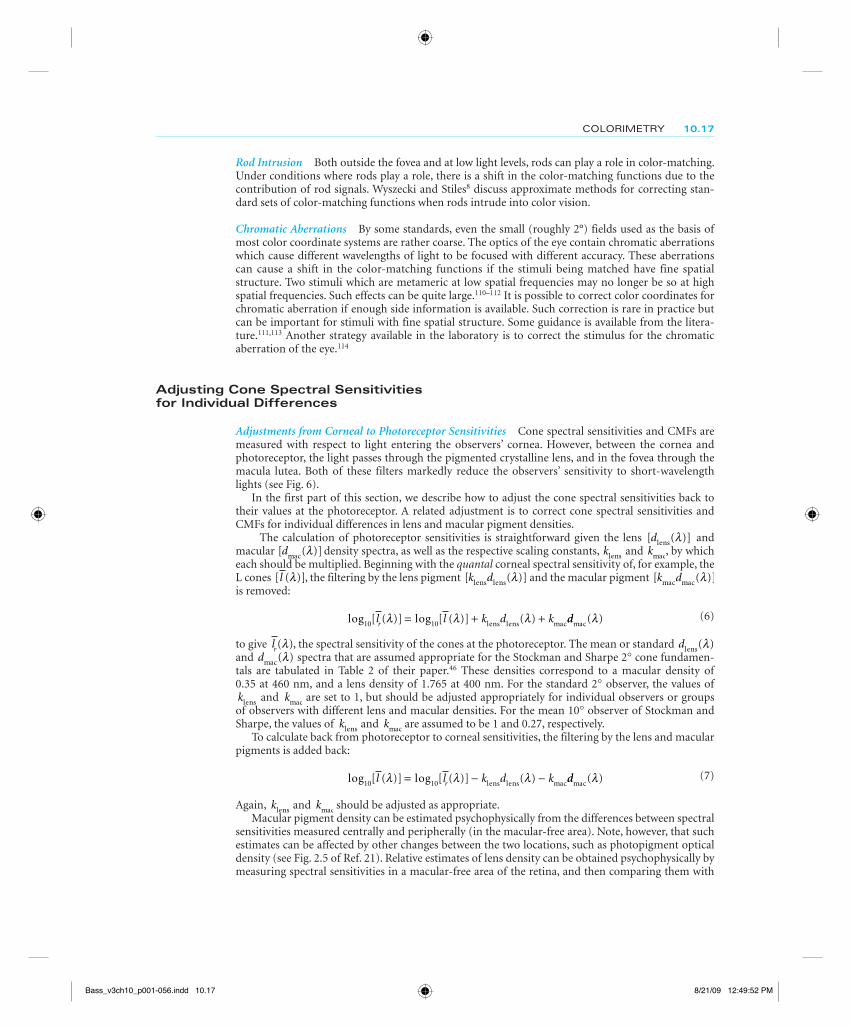
Adjusting Cone Spectral Sensitivities for Individual Differences
Adjustments from Corneal to Photoreceptor Sensitivities Cone spectral sensitivities and CMFs are measured with respect to light entering the observers’ cornea. However, between the cornea and photoreceptor, the light passes through the pigmented crystalline lens, and in the fovea through the macula lutea. Both of these filters markedly reduce the observers’ sensitivity to short-wavelength lights (see Fig. 6).
In the first part of this section, we describe how to adjust the cone spectral sensitivities back to their values at the photoreceptor. A related adjustment is to correct cone spectral sensitivities and CMFs for individual differences in lens and macular pigment densities.
The calculation of photoreceptor sensitivities is straightforward given the lens [ ( )]dlens λ and macular [ ( )]dmac λ density spectra, as well as the respective scaling constants, klens and kmac, by which each should be multiplied. Beginning with the quantal corneal spectral sensitivity of, for example, the L cones [ ( )]l λ , the filtering by the lens pigment [ ( )]k dlens lens λ and the macular pigment [ ( )]k dmac mac λ is removed:
log [ ( )] log [ ( )] ( )10 10l l k d kr λ λ λ= + +lens lens macddmac( )λ (6)
to give lr( )λ , the spectral sensitivity of the cones at the photoreceptor. The mean or standard dlens( )λ and dmac( )λ spectra that are assumed appropriate for the Stockman and Sharpe 2° cone fundamen-tals are tabulated in Table 2 of their paper.46 These densities correspond to a macular density of 0.35 at 460 nm, and a lens density of 1.765 at 400 nm. For the standard 2° observer, the values of klens and kmac are set to 1, but should be adjusted appropriately for individual observers or groups of observers with different lens and macular densities. For the mean 10° observer of Stockman and Sharpe, the values of klens and kmac are assumed to be 1 and 0.27, respectively.
To calculate back from photoreceptor to corneal sensitivities, the filtering by the lens and macular pigments is added back:
log [ ( )] log [ ( )] ( )10 10l l k d krλ λ λ= − −lens lens macddmac( )λ (7)
Again, klens and kmac should be adjusted as appropriate.Macular pigment density can be estimated psychophysically from the differences between spectral
sensitivities measured centrally and peripherally (in the macular-free area). Note, however, that such estimates can be affected by other changes between the two locations, such as photopigment optical density (see Fig. 2.5 of Ref. 21). Relative estimates of lens density can be obtained psychophysically by measuring spectral sensitivities in a macular-free area of the retina, and then comparing them with
Bass_v3ch10_p001-056.indd 10.17Bass_v3ch10_p001-056.indd 10.17 8/21/09 12:49:52 PM8/21/09 12:49:52 PM
10.18 VISION AND VISION OPTICS
mean spectral sensitivity data. Typically, rod spectral sensitivities are measured115 and then compared with mean rod data, such as the data for 50 observers measured by Crawford72 to obtain the mean standard rod spectral sensitivity function, V ′(l). Absolute lens density estimates can be obtained by comparing spectral sensitivities with photopigment spectra. See Ref. 21 for discussion.
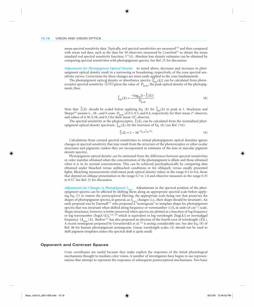
Adjustments for Photopigment Optical Density As noted above, decreases and increases in phot-opigment optical density result in a narrowing or broadening, respectively, of the cone spectral sen-sitivity curves. Corrections for these changes are most easily applied to the cone fundamentals.
The photopigment optical density or absorbance spectra [ ( )]lOD λ can be calculated from photo-receptor spectral sensitivity [ ( )]lr λ given the value of Dpeak, the peak optical density of the photopig-ment, thus:
ll
Dr
ODpeak
( )log [ ( )]
λλ
=− −10 1
(8)
Note that lr( )λ should be scaled before applying Eq. (8) for lOD( )λ to peak at 1. Stockman and Sharpe46 assume L-, M-, and S-cone Dpeak of 0.5, 0.5, and 0.4, respectively, for their mean 2° observer, and values of 0.38, 0.38, and 0.3 for their mean 10° observer.
The spectral sensitivity at the photoreceptor, lr( )λ , can be calculated from the normalized phot-opigment optical density spectrum, lOD( )λ , by the inversion of Eq. (8) (see Ref. 116):
lrD l( ) ( )λ λ= − −1 10 peak OD (9)
Calculations from corneal spectral sensitivities to retinal photopigment optical densities ignore changes in spectral sensitivity that may result from the structure of the photoreceptor or other ocular structures and pigments (unless they are incorporated in estimates of the lens or macular pigment density spectra).
Photopigment optical density can be estimated from the differences between spectral sensitivities or color matches obtained when the concentration of the photopigment is dilute and those obtained when it is in its normal concentration. This can be achieved psychophysically by comparing data obtained under bleached versus unbleached conditions or for obliquely versus axially presented lights. Bleaching measurements yield mean peak optical density values in the range 0.3 to 0.6, those that depend on oblique presentation in the range 0.7 to 1.0 and objective measures in the range 0.35 to 0.57. See Ref. 21 for discussion.
Adjustments for Changes in Photopigment lmax Adjustments in the spectral position of the phot-opigment spectra can be affected by shifting them along an appropriate spectral scale before apply-ing Eq. (7) to restore the prereceptoral filtering, the appropriate scale being one that preserves the shapes of photopigment spectra, in general, as lmax changes (i.e., their shape should be invariant). An early proposal was by Dartnall117 who proposed a “nomogram” or template shape for photopigment spectra that was invariant when shifted along frequency or wavenumber (1/l, in units of cm–1) scale. Shape invariance, however, is better preserved when spectra are plotted as a function of log frequency or log wavenumber [log( / )]1 λ ,118–120 which is equivalent to log wavelength [log( )]λ or normalized frequency ( / ).maxλ λ Barlow121 has also proposed an abscissa of the fourth root of wavelength ( λ4 ).A recent nomogram proposed by Govardovskii et al.122 is seeing considerable use. See also Eq. (8) of Ref. 46 for human photopigment nomograms. Linear wavelength scales (l) should not be used to shift pigment templates unless the spectral shift is quite small.
Opponent and Contrast Spaces
Cone coordinates are useful because they make explicit the responses of the initial physiological mechanisms thought to mediate color vision. A number of investigators have begun to use represen-tations that attempt to represent the responses of subsequent postreceptoral mechanisms. Two basic
Bass_v3ch10_p001-056.indd 10.18Bass_v3ch10_p001-056.indd 10.18 8/21/09 12:49:52 PM8/21/09 12:49:52 PM
COLORIMETRY 10.19
ideas underlie these representations. The first is the general opponent processing model described in companion chapter (Chap. 11) in this volume. We call representations based on this idea opponent color spaces. The second idea is that stimulus contrast is more relevant than stimulus magnitude.123 We call spaces that are based on this second idea modulation or contrast color spaces. Some color spaces are both opponent and contrast color spaces.
Cone contrast space To derive coordinates in the cone contrast color space, the stimulus is first expressed in terms of its cone coordinates. The cone coordinates of a white point are then chosen. Usually these are the cone coordinates of a uniform adapting field or the spatio-temporal average of the cone coordinates of the entire image sequence. The cone coordinates of the white point are subtracted from the cone coordinates of the stimulus and the resulting differences are normalized by the corresponding cone coordinates of the white point.
The DKL color space Derrington, Krauskopf, and Lennie124 introduced an opponent modulation space that is now widely used. This space is closely related to the chromaticity diagram suggested by MacLeod and Boynton125 (see also Ref. 126). To derive coordinates in the DKL color space, the stimulus is first expressed in cone coordinates. As with cone contrast space, the cone coordinates of a white point are then subtracted from the cone coordinates of the stimulus of interest. The next step is to reexpress the resulting difference as tristimulus values with respect to a new choice of primaries that are thought to isolate the responses of post-receptoral mechanisms.127,128 The three primaries are chosen so that modulating two of them does not change the response of the photopic luminance mechanism (see section “Brightness Matching and Photometry”). The color coordinates corre-sponding to these two primaries are often called the constant B and constant R and G coordinates. Modulating the constant R and G coordinates of a stimulus modulates only the S cones. Modulating the constant B coordinate modulates both the L and M cones but keeps the S-cone response con-stant. Because the constant R and G coordinates are not allowed to change the response of the phot-opic luminance mechanism, the DKL color space is well-defined only if the S cones do not contribute to luminance. The third primary of the space is chosen so that it has the same relative cone coordi-nates as the white point. The coordinate corresponding to this third primary is called the luminance coordinate. Flitcroft110 and Brainard129 provide detailed treatments of the DKL color space.
Caveats The basic ideas underlying the use of opponent and modulation/contrast color spaces seem to be valid. On the other hand, there is not a general agreement about how signals from cones are combined into opponent channels, about how this combination depends on adaptation, or about how adaptation affects signals originating in the cones. Since a specific model of these processes is implicit in any opponent or modulation/contrast color space, coordinates in these spaces must be treated carefully. This is particularly true of contrast spaces, where the relation between the physical stimulus and coordinates in the space depends on the choice of white point. As a consequence, radi-cally different stimuli can have identical coordinates in a contrast space. For example, 100 percent contrast monochromatic intensity gratings are all represented by the same coordinates in contrast color spaces, independent of their wavelength. Nonetheless, such stimuli appear very different to human observers. Identity of coordinates in a contrast color space does not imply identity of appear-ance across different choices of white points. See Ref. 129 for more extended discussion.
Visualizing Color Data
A challenge facing today’s color scientist is to produce and interpret graphical representations of color data. Because color coordinates are three-dimensional, it is difficult to plot them on a two-dimensional page. Even more difficult is to represent a dependent measure of visual performance as a function of color coordinates. We discuss several approaches.
Three-Dimensional Approaches One strategy is to plot the three-dimensional data in perspective. In many cases the projection viewpoint may be chosen to provide a clear view of the regularities of
Bass_v3ch10_p001-056.indd 10.19Bass_v3ch10_p001-056.indd 10.19 8/21/09 12:49:53 PM8/21/09 12:49:53 PM
10.20 VISION AND VISION OPTICS
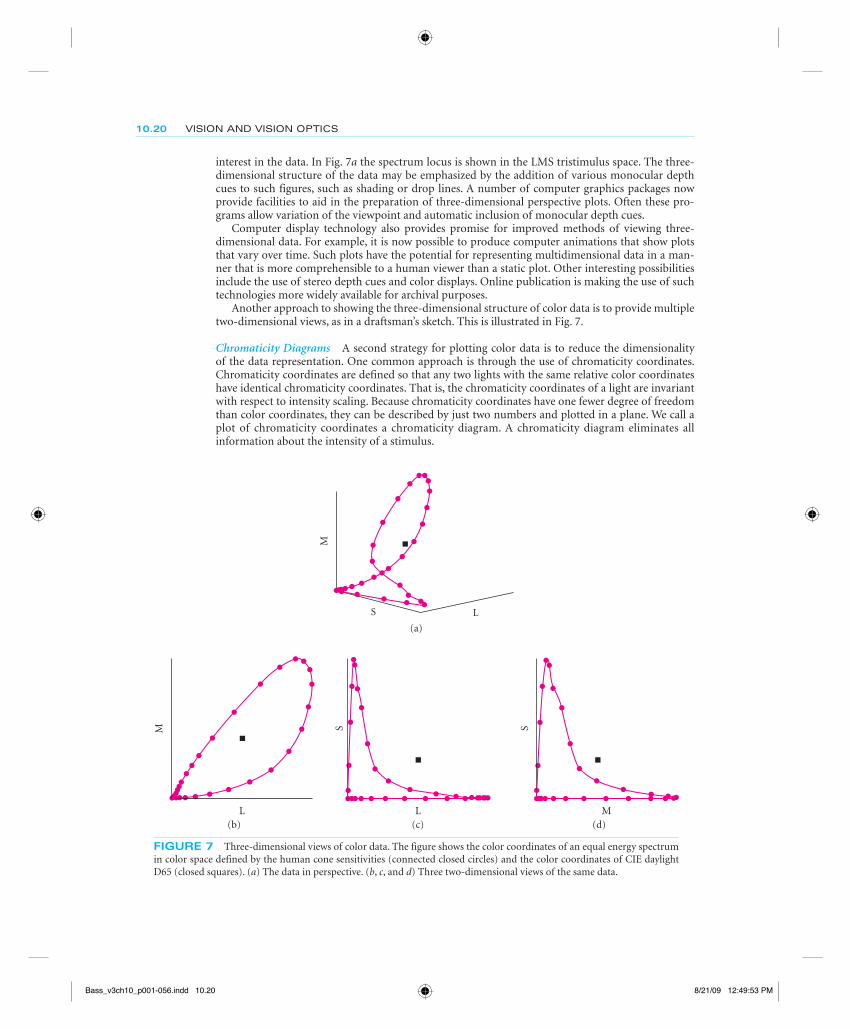
interest in the data. In Fig. 7a the spectrum locus is shown in the LMS tristimulus space. The three-dimensional structure of the data may be emphasized by the addition of various monocular depth cues to such figures, such as shading or drop lines. A number of computer graphics packages now provide facilities to aid in the preparation of three-dimensional perspective plots. Often these pro-grams allow variation of the viewpoint and automatic inclusion of monocular depth cues.
Computer display technology also provides promise for improved methods of viewing three-dimensional data. For example, it is now possible to produce computer animations that show plots that vary over time. Such plots have the potential for representing multidimensional data in a man-ner that is more comprehensible to a human viewer than a static plot. Other interesting possibilities include the use of stereo depth cues and color displays. Online publication is making the use of such technologies more widely available for archival purposes.
Another approach to showing the three-dimensional structure of color data is to provide multiple two-dimensional views, as in a draftsman’s sketch. This is illustrated in Fig. 7.
Chromaticity Diagrams A second strategy for plotting color data is to reduce the dimensionality of the data representation. One common approach is through the use of chromaticity coordinates. Chromaticity coordinates are defined so that any two lights with the same relative color coordinates have identical chromaticity coordinates. That is, the chromaticity coordinates of a light are invariant with respect to intensity scaling. Because chromaticity coordinates have one fewer degree of freedom than color coordinates, they can be described by just two numbers and plotted in a plane. We call a plot of chromaticity coordinates a chromaticity diagram. A chromaticity diagram eliminates all information about the intensity of a stimulus.
M
S L
M
L L M
SS
(b)
(a)
(c) (d)
FIGURE 7 Three-dimensional views of color data. The figure shows the color coordinates of an equal energy spectrum in color space defined by the human cone sensitivities (connected closed circles) and the color coordinates of CIE daylight D65 (closed squares). (a) The data in perspective. (b, c, and d) Three two-dimensional views of the same data.
Bass_v3ch10_p001-056.indd 10.20Bass_v3ch10_p001-056.indd 10.20 8/21/09 12:49:53 PM8/21/09 12:49:53 PM
COLORIMETRY 10.21
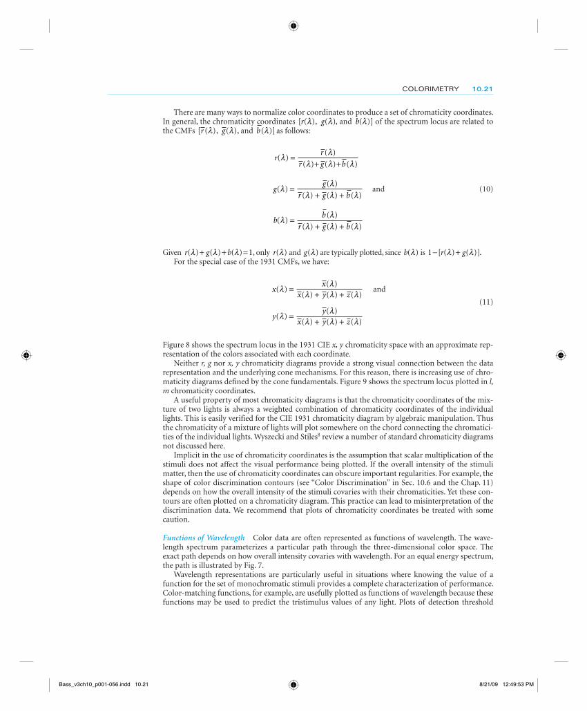
There are many ways to normalize color coordinates to produce a set of chromaticity coordinates. In general, the chromaticity coordinates [ ( )r λ , g( )λ , and b( )]λ of the spectrum locus are related to the CMFs [ ( )r λ , g( )λ , and b( )]λ as follows:
rr
r g b( )
( )
( ) ( ) ( )λ λ
λ λ λ=
+ +
gg
r g b( )
( )
( ) ( ) ( )λ λ
λ λ λ=
+ + and (10)
bb
r g b( )
( )
( ) ( ) ( )λ λ
λ λ λ=
+ +
Given r g b( ) ( ) ( )λ λ λ+ + =1, only r( )λ and g( )λ are typically plotted, since b( )λ is 1− +[ ( ) ( )].r gλ λFor the special case of the 1931 CMFs, we have:
xx
x y z( )
( )( ) ( ) ( )
λ λλ λ λ
=+ +
and
(11)
yy
x y z( )
( )( ) ( ) ( )
λ λλ λ λ
=+ +
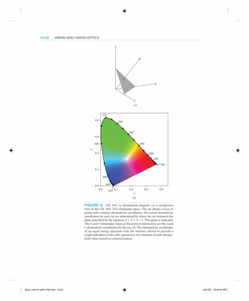
Figure 8 shows the spectrum locus in the 1931 CIE x, y chromaticity space with an approximate rep-resentation of the colors associated with each coordinate.
Neither r, g nor x, y chromaticity diagrams provide a strong visual connection between the data representation and the underlying cone mechanisms. For this reason, there is increasing use of chro-maticity diagrams defined by the cone fundamentals. Figure 9 shows the spectrum locus plotted in l, m chromaticity coordinates.
A useful property of most chromaticity diagrams is that the chromaticity coordinates of the mix-ture of two lights is always a weighted combination of chromaticity coordinates of the individual lights. This is easily verified for the CIE 1931 chromaticity diagram by algebraic manipulation. Thus the chromaticity of a mixture of lights will plot somewhere on the chord connecting the chromatici-ties of the individual lights. Wyszecki and Stiles8 review a number of standard chromaticity diagrams not discussed here.
Implicit in the use of chromaticity coordinates is the assumption that scalar multiplication of the stimuli does not affect the visual performance being plotted. If the overall intensity of the stimuli matter, then the use of chromaticity coordinates can obscure important regularities. For example, the shape of color discrimination contours (see “Color Discrimination” in Sec. 10.6 and the Chap. 11) depends on how the overall intensity of the stimuli covaries with their chromaticities. Yet these con-tours are often plotted on a chromaticity diagram. This practice can lead to misinterpretation of the discrimination data. We recommend that plots of chromaticity coordinates be treated with some caution.
Functions of Wavelength Color data are often represented as functions of wavelength. The wave-length spectrum parameterizes a particular path through the three-dimensional color space. The exact path depends on how overall intensity covaries with wavelength. For an equal energy spectrum, the path is illustrated by Fig. 7.
Wavelength representations are particularly useful in situations where knowing the value of a function for the set of monochromatic stimuli provides a complete characterization of performance. Color-matching functions, for example, are usefully plotted as functions of wavelength because these functions may be used to predict the tristimulus values of any light. Plots of detection threshold
Bass_v3ch10_p001-056.indd 10.21Bass_v3ch10_p001-056.indd 10.21 8/21/09 12:49:53 PM8/21/09 12:49:53 PM
10.22 VISION AND VISION OPTICS
x0.0 0.2 0.4 0.6 0.8
0.0
0.2
0.4
0.6
0.8
520
560
540
580500
600
y
620
700
480
460
420
X
Z
Y
(a)
(b)
FIGURE 8 CIE 1931 xy chromaticity diagram. (a) A perspective view of the CIE 1931 XYZ tristimulus space. The ray shows a locus of points with constant chromaticity coordinates. The actual chromaticity coordinates for each ray are determined by where the ray intersects the plane described by the equation X + Y + Z = 1. This plane is indicated. The X and Y tristimulus values at the point of intersection are the x and y chromaticity coordinates for the ray. (b) The chromaticity coordinates of an equal energy spectrum with the interior colored to provide a rough indication of the color appearance of a stimulus of each chroma-ticity when viewed in a neutral context.
Bass_v3ch10_p001-056.indd 10.22Bass_v3ch10_p001-056.indd 10.22 8/21/09 12:49:54 PM8/21/09 12:49:54 PM
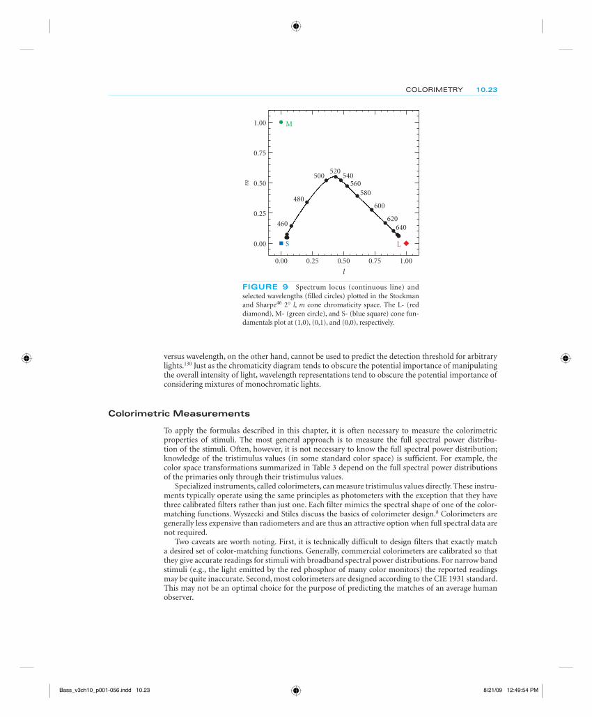
COLORIMETRY 10.23
versus wavelength, on the other hand, cannot be used to predict the detection threshold for arbitrary lights.130 Just as the chromaticity diagram tends to obscure the potential importance of manipulating the overall intensity of light, wavelength representations tend to obscure the potential importance of considering mixtures of monochromatic lights.
Colorimetric Measurements
To apply the formulas described in this chapter, it is often necessary to measure the colorimetric properties of stimuli. The most general approach is to measure the full spectral power distribu-tion of the stimuli. Often, however, it is not necessary to know the full spectral power distribution; knowledge of the tristimulus values (in some standard color space) is sufficient. For example, the color space transformations summarized in Table 3 depend on the full spectral power distributions of the primaries only through their tristimulus values.
Specialized instruments, called colorimeters, can measure tristimulus values directly. These instru-ments typically operate using the same principles as photometers with the exception that they have three calibrated filters rather than just one. Each filter mimics the spectral shape of one of the color-matching functions. Wyszecki and Stiles discuss the basics of colorimeter design.8 Colorimeters are generally less expensive than radiometers and are thus an attractive option when full spectral data are not required.
Two caveats are worth noting. First, it is technically difficult to design filters that exactly match a desired set of color-matching functions. Generally, commercial colorimeters are calibrated so that they give accurate readings for stimuli with broadband spectral power distributions. For narrow band stimuli (e.g., the light emitted by the red phosphor of many color monitors) the reported readings may be quite inaccurate. Second, most colorimeters are designed according to the CIE 1931 standard. This may not be an optimal choice for the purpose of predicting the matches of an average human observer.
l
0.00 0.25 0.50 0.75 1.00
0.00
0.25
0.50
0.75
1.00
500
640
520
480
560540
460
M
L
580
600
620
Sm
FIGURE 9 Spectrum locus (continuous line) and selected wavelengths (filled circles) plotted in the Stockman and Sharpe46 2° l, m cone chromaticity space. The L- (red diamond), M- (green circle), and S- (blue square) cone fun-damentals plot at (1,0), (0,1), and (0,0), respectively.
Bass_v3ch10_p001-056.indd 10.23Bass_v3ch10_p001-056.indd 10.23 8/21/09 12:49:54 PM8/21/09 12:49:54 PM
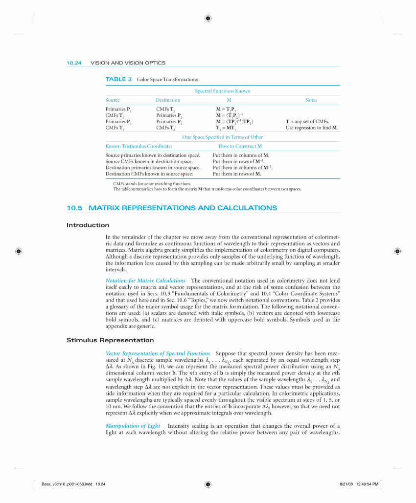
10.24 VISION AND VISION OPTICS
10.5 MATRIX REPRESENTATIONS AND CALCULATIONS
Introduction
In the remainder of the chapter we move away from the conventional representation of colorimet-ric data and formulae as continuous functions of wavelength to their representation as vectors and matrices. Matrix algebra greatly simplifies the implementation of colorimetry on digital computers. Although a discrete representation provides only samples of the underlying function of wavelength, the information loss caused by this sampling can be made arbitrarily small by sampling at smaller intervals.
Notation for Matrix Calculations The conventional notation used in colorimetry does not lend itself easily to matrix and vector representations, and at the risk of some confusion between the notation used in Secs. 10.3 “Fundamentals of Colorimetry” and 10.4 “Color Coordinate Systems” and that used here and in Sec. 10.6 “Topics,” we now switch notational conventions. Table 2 provides a glossary of the major symbol usage for the matrix formulation. The following notational conven-tions are used: (a) scalars are denoted with italic symbols, (b) vectors are denoted with lowercase bold symbols, and (c) matrices are denoted with uppercase bold symbols. Symbols used in the appendix are generic.
Stimulus Representation
Vector Representation of Spectral Functions Suppose that spectral power density has been mea-sured at Nl discrete sample wavelengths l1 . . . lNl
, each separated by an equal wavelength step Δl. As shown in Fig. 10, we can represent the measured spectral power distribution using an Nl dimensional column vector b. The nth entry of b is simply the measured power density at the nth sample wavelength multiplied by Δl. Note that the values of the sample wavelengths l1 . . .
lNl and
wavelength step Δl are not explicit in the vector representation. These values must be provided as side information when they are required for a particular calculation. In colorimetric applications, sample wavelengths are typically spaced evenly throughout the visible spectrum at steps of 1, 5, or 10 nm. We follow the convention that the entries of b incorporate Δl, however, so that we need not represent Δl explicitly when we approximate integrals over wavelength.
Manipulation of Light Intensity scaling is an operation that changes the overall power of a light at each wavelength without altering the relative power between any pair of wavelengths.
TABLE 3 Color Space Transformations
Spectral Functions Known
Source Destination M Notes
Primaries P1 CMFs T2 M = T2P1CMFs T1 Primaries P2 M = (T1P2)
–1
Primaries P1 Primaries P2 M = (TP2)–1(TP1) T is any set of CMFs.
CMFs T1 CMFs T2 T2 = MT1 Use regression to find M.
One Space Specified in Terms of Other
Known Tristimulus Coordinates How to Construct M
Source primaries known in destination space. Put them in columns of M.Source CMFs known in destination space. Put them in rows of M–1.Destination primaries known in source space. Put them in columns of M–1.Destination CMFs known in source space. Put them in rows of M.
CMFs stands for color matching functions.The table summarizes how to form the matrix M that transforms color coordinates between two spaces.
Bass_v3ch10_p001-056.indd 10.24Bass_v3ch10_p001-056.indd 10.24 8/21/09 12:49:54 PM8/21/09 12:49:54 PM

COLORIMETRY 10.25
The superposition of two lights is an operation that produces a new light whose power at each wavelength is the sum of the power in the original lights at the corresponding wavelength. The effects of both manipulations may be expressed using matrix algebra.
We use scalar multiplication to represent intensity scaling. If a light b1 is scaled by a factor a, then the result b is given by the equation b = b1a. The expression b1a represents a vector whose entries are obtained by multiplying the entries of the vector b1 by the scalar a. Similarly, we use vector addition to represent superposition. If we superimpose two lights b1 and b2, then the result b is given by the equation b = b1 + b2. The expression b1 + b2 represents a vector whose entries are obtained by adding the entries of the vectors b1 and b2 component by component. Figures 11 and 12 depict both of these operations.
0
500
1000
1500
400 450 500P
ower
(ar
bitr
ary
un
its)
550 600 650 700
Wavelength (nm)
b =
b1b2
•••
b31
FIGURE 10 The vector representation of functions of wavelength. The plot shows a spectral power distribution measured at 10-nm inter-vals between 400 and 700 nm. Each point on the plot represents the power at a single sample wavelength. The vector b on the right depicts the vector representation of the same spectral power distribution. The nth entry of b is simply the measured power density at the nth sample wave-length times Δl. Thus b1 is derived from the power density at 400 nm, b2 is derived from the power density at 410 nm, and b31 is derived from the power density at 700 nm.
0
500
1000
1500
400 450 500
Pow
er (
arbi
trar
y u
nit
s)
550 600 650 700Wavelength (nm)
b1
b
•••
b
•••
= 0.5
•••
b1
•••
FIGURE 11 Representation of intensity scaling. Suppose that light b is created by reducing the power in light b1 by a factor of 0.5 at each wave-length. The result is shown graphically in the plot. The vector representation of the same relation is given by the equation b = b10.5.
Bass_v3ch10_p001-056.indd 10.25Bass_v3ch10_p001-056.indd 10.25 8/21/09 12:49:55 PM8/21/09 12:49:55 PM

10.26 VISION AND VISION OPTICS
Linear Models for Spectral Functions Intensity scaling and superposition may be used in combina-tion to produce a wide range of spectral functions. Suppose that we have a set of Nb lights that we can individually scale and superimpose. Let the vectors b1 . . .
bNb represent the spectral power distribu-
tions of these lights. In this case, we can produce any spectral power distribution b that has the form
b = b1a1 + . . . + bNbaNb
(12)
Now suppose we know that a spectral function b is constrained to have the form of Eq. (12) where the vectors b1 . . . bNb
are known. Then we can specify b completely by providing the values of the scalars a1 . . . aNb
. If the number of primaries Nb is less than the number of sample wavelengths Nl, then this specification is more efficient (i.e., requires fewer numbers) than specifying the entries of b directly. We say that the spectral functions that satisfy Eq. (12) are described by (or lie within) a linear model. We call Nb the dimension of the linear model. We call the vectors b1 . . . bNb the basis vectors for the model. We call the scalars a1 . . . aNb
required to construct any particular spectral function the model weights for that function.
Matrix Representation of Linear Models Equation (12) can be written using vector and matrix nota-tion. Let B be an Nl by Nb dimensional matrix whose columns are the basis vectors b1 . . . bNb
. We call B the basis matrix for the linear model. The composition of the basis matrix is shown pictorially on the left of Fig. 13. Let a be an Nb dimensional vector whose entries are the weights a1 . . . aNb
. Figure 13 also depicts the vector a. Using B and a we can re-express Eq. (12) as the matrix multiplication
b = Ba (13)
The equivalence of Eqs. (12) and (13) may be established by direct expansion of the definition of matrix multiplication (see App. A). A useful working intuition for matrix multiplication is that the effect of multiplying a matrix times a vector (e.g., Ba) is to produce a new vector (e.g., b) that is a weighted superposition of the columns of the matrix (e.g., B), where the weight for column bi is given by the ith weight, ai, in a.
Use of Linear Models When we know that a spectral function is described by a linear model, we can specify it by using the weight vector a. The matrix B, which is determined by the basis vectors, specifies the side information necessary to convert the vector a back to the discrete wavelength
0
1000
2000
3000
400 450 500
Pow
er (
arbi
trar
y u
nit
s)
550 600 650 700
Wavelength (nm)
b1
b2
b •••
b
•••
= +
•••
b1
•••
•••
b2
•••
FIGURE 12 Representation of superposition. Suppose that light b is cre-ated by superimposing two lights b1 and b2. The result is shown graphically in the plot. The vector representation of the same relation is given by the equation b = b1 + b2.
Bass_v3ch10_p001-056.indd 10.26Bass_v3ch10_p001-056.indd 10.26 8/21/09 12:49:55 PM8/21/09 12:49:55 PM
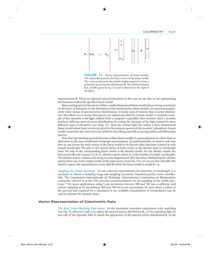
COLORIMETRY 10.27
representation b. When we represent spectral functions in this way, we say that we are representing the functions within the specified linear model.
Representing spectral functions within a small-dimensional linear model places strong constraints on the form of functions. As the dimension of the model grows, linear models can represent progres-sively wider classes of spectral power distributions. In many cases of interest, there is prior informa-tion that allows us to assume that spectra are indeed described by a linear model. A common exam-ple of this situation is the light emitted from a computer controlled color monitor. Such a monitor produces different spectral power distributions by scaling the intensity of the light emitted by three different types of phosphor (see Chap. 22). Thus the emitted light lies within a three-dimensional linear model whose basis vectors are given by the emission spectra of the monitor’s phosphors. Linear model constraints also turn out to be useful for describing naturally occurring surface and illuminant spectra.
Note that representing spectral functions within linear models is a generalization of, rather than an alternative to, the more traditional wavelength representation. To understand this, we need to only note that we can choose the basis vectors of the linear model to be discrete delta functions centered at each sample wavelength. We refer to this special choice of basis vectors as the identity basis or wavelength basis. We refer to the corresponding linear model as the identity model. For the identity model, the basis matrix B is the (square) Nl by Nl identity matrix, where Nl is the number of sample wavelengths. The identity matrix contains ones along its main diagonal and zeros elsewhere. Multiplying the identity matrix times any vector simply results in the same vector. From Eq. (13), we can see that when B is the identity matrix, the representation of any light b within the linear model is simply b = a.
Sampling the Visible Spectrum To use a discrete representation for functions of wavelength, it is necessary to choose a sampling range and sampling increment. Standard practice varies consider-ably. The Commission Internationale de l’Éclairage (International Commission on Illumination, commonly referred to as the CIE) provides recommendations on the sampling of the visible spec-trum.10 For many applications, using 5-nm increments between 380 and 780 nm is sufficient, and coarser sampling at 10 nm between 400 and 700 nm is not uncommon. In cases where a subset of the spectral data required for a calculation is not available, interpolation or extrapolation may be used to estimate the missing values.
Vector Representation of Colorimetric Data
The Basic Color-Matching Experiment In the maximum saturation experiment color matching (see Fig. 3), observer’s task is to adjust the spectral power distribution bm of the matching light on one side of the bipartite field to match the appearance of the spectral power distribution bt of the
B = b1b2 bNb
a =
a1
a2
aNb
b = Ba
• • •
FIGURE 13 Vector representation of linear models. The matrix B represents the basis vectors of the linear model. The vector a represents the model weights required to form a particular spectral power distribution b. The relation between b, a, and B is given by Eq. (13) and is depicted on the right of the figure.
Bass_v3ch10_p001-056.indd 10.27Bass_v3ch10_p001-056.indd 10.27 8/21/09 12:49:55 PM8/21/09 12:49:55 PM
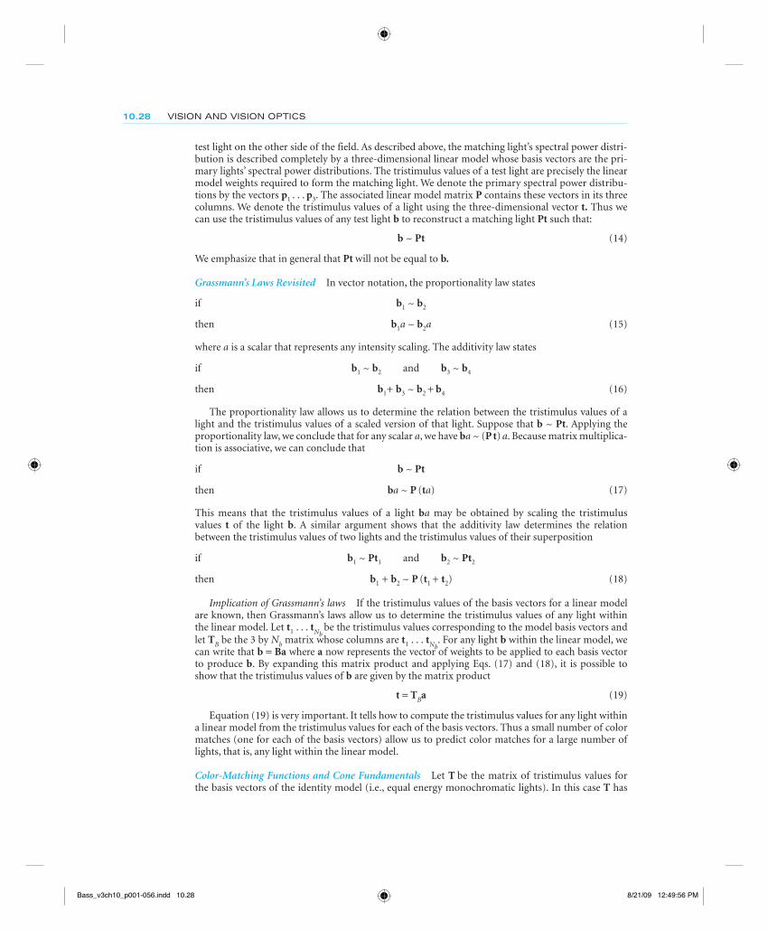
10.28 VISION AND VISION OPTICS
test light on the other side of the field. As described above, the matching light’s spectral power distri-bution is described completely by a three-dimensional linear model whose basis vectors are the pri-mary lights’ spectral power distributions. The tristimulus values of a test light are precisely the linear model weights required to form the matching light. We denote the primary spectral power distribu-tions by the vectors p1 . . .
p3. The associated linear model matrix P contains these vectors in its three columns. We denote the tristimulus values of a light using the three-dimensional vector t. Thus we can use the tristimulus values of any test light b to reconstruct a matching light Pt such that:
b ~ Pt (14)
We emphasize that in general that Pt will not be equal to b.
Grassmann’s Laws Revisited In vector notation, the proportionality law states
if b1 ~ b2
then b1a ~ b2a (15)
where a is a scalar that represents any intensity scaling. The additivity law states
if b1 ~ b2 and b3 ~ b4
then b1+ b3 ~ b2 + b4 (16)
The proportionality law allows us to determine the relation between the tristimulus values of a light and the tristimulus values of a scaled version of that light. Suppose that b ~ Pt. Applying the proportionality law, we conclude that for any scalar a, we have ba ~ (P t) a. Because matrix multiplica-tion is associative, we can conclude that
if b ~ Pt
then ba ~ P (ta) (17)
This means that the tristimulus values of a light ba may be obtained by scaling the tristimulusvalues t of the light b. A similar argument shows that the additivity law determines the relation between the tristimulus values of two lights and the tristimulus values of their superposition
if b1 ~ Pt1 and b2 ~ Pt2
then b1 + b2 ~ P (t1 + t2) (18)
Implication of Grassmann’s laws If the tristimulus values of the basis vectors for a linear model are known, then Grassmann’s laws allow us to determine the tristimulus values of any light within the linear model. Let t1 . . . tNb
be the tristimulus values corresponding to the model basis vectors and let TB be the 3 by Nb matrix whose columns are t1 . . . tNb
. For any light b within the linear model, we can write that b = Ba where a now represents the vector of weights to be applied to each basis vector to produce b. By expanding this matrix product and applying Eqs. (17) and (18), it is possible to show that the tristimulus values of b are given by the matrix product
t = TBa (19)
Equation (19) is very important. It tells how to compute the tristimulus values for any light within a linear model from the tristimulus values for each of the basis vectors. Thus a small number of color matches (one for each of the basis vectors) allow us to predict color matches for a large number of lights, that is, any light within the linear model.
Color-Matching Functions and Cone Fundamentals Let T be the matrix of tristimulus values for the basis vectors of the identity model (i.e., equal energy monochromatic lights). In this case T has
Bass_v3ch10_p001-056.indd 10.28Bass_v3ch10_p001-056.indd 10.28 8/21/09 12:49:56 PM8/21/09 12:49:56 PM
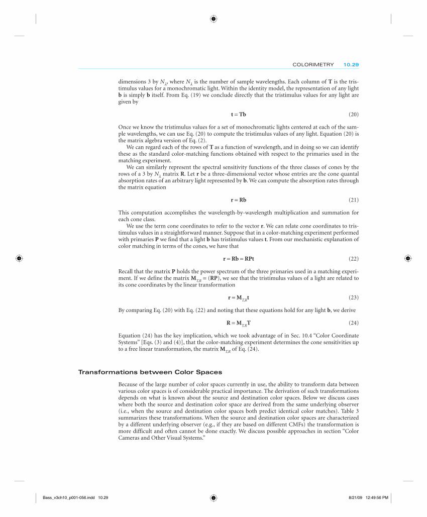
COLORIMETRY 10.29
dimensions 3 by Nl, where Nl is the number of sample wavelengths. Each column of T is the tris-timulus values for a monochromatic light. Within the identity model, the representation of any light b is simply b itself. From Eq. (19) we conclude directly that the tristimulus values for any light are given by
t = Tb (20)
Once we know the tristimulus values for a set of monochromatic lights centered at each of the sam-ple wavelengths, we can use Eq. (20) to compute the tristimulus values of any light. Equation (20) is the matrix algebra version of Eq. (2).
We can regard each of the rows of T as a function of wavelength, and in doing so we can identify these as the standard color-matching functions obtained with respect to the primaries used in the matching experiment.
We can similarly represent the spectral sensitivity functions of the three classes of cones by the rows of a 3 by Nl matrix R. Let r be a three-dimensional vector whose entries are the cone quantal absorption rates of an arbitrary light represented by b. We can compute the absorption rates through the matrix equation
r = Rb (21)
This computation accomplishes the wavelength-by-wavelength multiplication and summation for each cone class.
We use the term cone coordinates to refer to the vector r. We can relate cone coordinates to tris-timulus values in a straightforward manner. Suppose that in a color-matching experiment performed with primaries P we find that a light b has tristimulus values t. From our mechanistic explanation of color matching in terms of the cones, we have that
r = Rb = RPt (22)
Recall that the matrix P holds the power spectrum of the three primaries used in a matching experi-ment. If we define the matrix MT,R = (RP), we see that the tristimulus values of a light are related to its cone coordinates by the linear transformation
r = MT,Rt (23)
By comparing Eq. (20) with Eq. (22) and noting that these equations hold for any light b, we derive
R = MT,RT (24)
Equation (24) has the key implication, which we took advantage of in Sec. 10.4 “Color Coordinate Systems” [Eqs. (3) and (4)], that the color-matching experiment determines the cone sensitivities up to a free linear transformation, the matrix MT,R of Eq. (24).
Transformations between Color Spaces
Because of the large number of color spaces currently in use, the ability to transform data between various color spaces is of considerable practical importance. The derivation of such transformations depends on what is known about the source and destination color spaces. Below we discuss cases where both the source and destination color space are derived from the same underlying observer (i.e., when the source and destination color spaces both predict identical color matches). Table 3 summarizes these transformations. When the source and destination color spaces are characterized by a different underlying observer (e.g., if they are based on different CMFs) the transformation is more difficult and often cannot be done exactly. We discuss possible approaches in section “Color Cameras and Other Visual Systems.”
Bass_v3ch10_p001-056.indd 10.29Bass_v3ch10_p001-056.indd 10.29 8/21/09 12:49:56 PM8/21/09 12:49:56 PM
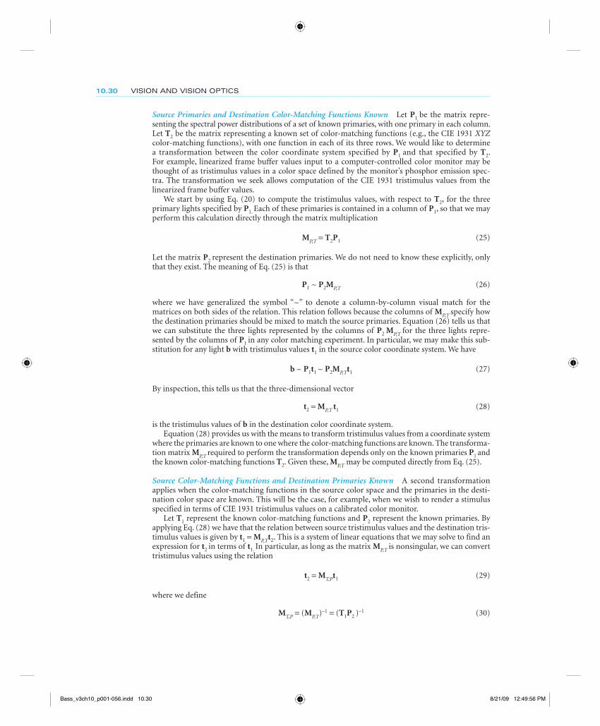
10.30 VISION AND VISION OPTICS
Source Primaries and Destination Color-Matching Functions Known Let P1 be the matrix repre-senting the spectral power distributions of a set of known primaries, with one primary in each column. Let T2 be the matrix representing a known set of color-matching functions (e.g., the CIE 1931 XYZ color-matching functions), with one function in each of its three rows. We would like to determine a transformation between the color coordinate system specified by P1 and that specified by T2. For example, linearized frame buffer values input to a computer-controlled color monitor may be thought of as tristimulus values in a color space defined by the monitor’s phosphor emission spec-tra. The transformation we seek allows computation of the CIE 1931 tristimulus values from the linearized frame buffer values.
We start by using Eq. (20) to compute the tristimulus values, with respect to T2, for the three primary lights specified by P1. Each of these primaries is contained in a column of P1, so that we may perform this calculation directly through the matrix multiplication
MP,T = T2P1 (25)
Let the matrix P2 represent the destination primaries. We do not need to know these explicitly, only that they exist. The meaning of Eq. (25) is that
P1 ~ P2MP,T (26)
where we have generalized the symbol “~” to denote a column-by-column visual match for the matrices on both sides of the relation. This relation follows because the columns of MP,T specify how the destination primaries should be mixed to match the source primaries. Equation (26) tells us that we can substitute the three lights represented by the columns of P2 MP,T for the three lights repre-sented by the columns of P1 in any color matching experiment. In particular, we may make this sub-stitution for any light b with tristimulus values t1 in the source color coordinate system. We have
b ~ P1t1 ~ P2MP,Tt1 (27)
By inspection, this tells us that the three-dimensional vector
t2 = MP,T t1 (28)
is the tristimulus values of b in the destination color coordinate system.Equation (28) provides us with the means to transform tristimulus values from a coordinate system
where the primaries are known to one where the color-matching functions are known. The transforma-tion matrix MP,T required to perform the transformation depends only on the known primaries P1 and the known color-matching functions T2. Given these, MP,T may be computed directly from Eq. (25).
Source Color-Matching Functions and Destination Primaries Known A second transformation applies when the color-matching functions in the source color space and the primaries in the desti-nation color space are known. This will be the case, for example, when we wish to render a stimulus specified in terms of CIE 1931 tristimulus values on a calibrated color monitor.
Let T1 represent the known color-matching functions and P2 represent the known primaries. By applying Eq. (28) we have that the relation between source tristimulus values and the destination tris-timulus values is given by t1 = MP,Tt2. This is a system of linear equations that we may solve to find an expression for t2 in terms of t1. In particular, as long as the matrix MP,T is nonsingular, we can convert tristimulus values using the relation
t2 = MT,Pt1 (29)
where we define
MT,P = (MP,T)–1 = (T1P2 )–1 (30)
Bass_v3ch10_p001-056.indd 10.30Bass_v3ch10_p001-056.indd 10.30 8/21/09 12:49:56 PM8/21/09 12:49:56 PM
COLORIMETRY 10.31
Source and Destination Primaries Known A third transformation applies when the primaries of both the source and destination color spaces are known. One application of this transformation is to generate matching stimuli on two different calibrated monitors.
Let P1 and P2 represent the two sets of primaries. Let T represent a set of color-matching functions for any human color coordinate system. (There is no requirement that the color-matching functions be related to either the source or the destination primaries. For example, the CIE 1931 XYZ color-matching functions might be used.) To do the conversion, we simply use Eq. (28) to transform from the color coordinate system described by P1 to the coordinate system described by T. Then we use Eq. (29) to transform from the coordinates system described by T to the coordinate system described by P2. The overall transformation is given by
t2 = MP,P t1 = (MT,P2)(MP1,T) t1 = (TP2)
–1 (TP1)t1 (31)
It should not be surprising that this transformation requires the specification of a set of color-matching functions. These color-matching functions are the only source of information about the human observer in the transformation equation.
Source and Destination Color-Matching Functions Known Finally, it is sometimes of interest to transform between two color spaces that are specified in terms of their color-matching functions. An example is transforming between the space defined by the Stiles and Burch 10° color-matching functions34 and the space defined by the Stockman and Sharpe 10° cone fundamentals.46
Let T1 and T2 represent the source and destination color-matching functions. Our development above assures us that there is some three-by-three transformation matrix, call it MT,T, that transforms color coordinates between the two systems. Recall that the columns of T1 and T2 are themselves tris-timulus values for corresponding monochromatic lights. Thus MT,T must satisfy
T2 = MT,TT1 (32)
This is a system of linear equations where the entries of MT,T are the unknown variables. This system may be solved using standard regression methods. Once we have solved for MT,T, we can transform tristimulus values using the equation
t2 = MT,T t1 (33)
The transformation specified by Eq. (33) will be exact as long as the two sets of color-matching functions T1 and T2 characterize the performance of the same observer. One sometimes wishes, how-ever, to transform between two color spaces that are defined with respect to different observers. For example, one might want to convert CIE 1931 XYZ tristimulus values to Judd-Vos modified tris-timulus values. Although the regression procedure described here will still produce a transformation matrix in this case, the result of the transformation is not guaranteed to be correct.4 We will return to this topic in section “Color Cameras and Other Visual Systems.”
Interpreting the Transformation Matrix It is useful to interpret the rows and columns of the matri-ces derived in the preceding sections. Let M be a matrix that maps the color coordinates from a source color space to a destination color space. Both source and destination color spaces are associated with a set of primaries and a set of color-matching functions. From our derivations above, we can conclude that the columns of M are the coordinates of the source primaries in the destination color space [see Eq. (25)] and the rows of M provide the destination color-matching functions with respect to the linear model whose basis functions are the primaries of source color space (see subsection “Use of Linear Modes” in Sec. 10.5). Similarly, the columns of M–1 are the coordinates of the destination pri-maries in the source color-matching space and the rows of M–1 are the source color-matching func-tions with respect to the linear model whose basis functions are the primaries of the destination color space. Thus in many cases it is possible to construct the matrix M without full knowledge of the spec-tral functions. This can be of practical importance. For example, monitor manufacturers often specify the CIE 1931 tristimulus values of their monitors’ phosphors. In addition, colorimeters that measure tristimulus values directly are often more readily available than spectral radiometers.
Bass_v3ch10_p001-056.indd 10.31Bass_v3ch10_p001-056.indd 10.31 8/21/09 12:49:57 PM8/21/09 12:49:57 PM
10.32 VISION AND VISION OPTICS
Transforming Primaries and Color-Matching Functions We have shown that color coordinates in any two color spaces may be related by applying a linear transformation M. The converse is also true. If we pick any nonsingular linear transformation M and apply it to a set of color coordinates we have defined a new color space that will successfully predict color matches. The color-matching functions for this new space will be given by T2 = MT1. A set of primaries for the new space will be given by P2 = P1M–1. These derived primaries are not unique. Any set of primaries that match the constructed primaries will also work.
The fact that new color spaces can be constructed by applying linear transformations has an important implication for the study of color. If we restrict attention to what we may conclude from the color-matching experiment, we can only determine the psychological representation of color up to a free linear transformation. There are two attitudes one can take toward this fact. The conservative attitude is to refrain from making any statements about the nature of color vision that depend on a particular choice of color space. The other is to appeal to experiments other than the color-matching experiment to choose a privileged representation.
10.6 TOPICS
Surfaces and Illuminants
As shown in Fig. 1, the light reaching the eye is often formed when light from an illuminant reflects from a surface. Illuminants and surfaces are of interest in color reproduction applications involving inks, paints, and dyes and in lighting design applications.
Reflection Model Illuminants are specified by their spectral power distributions. We will use the vector e to represent illuminant spectral power distributions. In general, the interaction of light with matter is quite complex. For many applications, however, a rather simple model is acceptable. Using this model, we describe a surface by its surface reflectance function. The surface reflectance function specifies, for each sample wavelength, the fraction of illuminant power that is reflected to the observer. We will use the vector s to represent surface reflectance spectra. Each entry of s gives the reflectance measured at a single sample wavelength. Thus the spectral power distribution b of the reflected light is given by the wavelength-by-wavelength product of the illuminant spectral power distribution and the surface reflectance function.
The most important consideration neglected in this formulation is viewing geometry. The relation between the radiant power emitted by a source of illumination, the material properties of a surface, and the radiant power reaching an observer can depend strongly on the viewing geometry. In our formulation, these geometrical factors must be incorporated implicitly into the specification of the illuminant and surface properties, so that any actual calculation is specific to a particular viewing geometry. Moreover, the surface reflectance must be understood as being associated with a particular image location, rather than with a particular object. A topic of current research in computer graph-ics is to find accurate and efficient ways to specify illuminants and surfaces for rendering,131,132 and parallel work in human vision seeks to understand how the reflectance of spatially complex objects is perceived.133–136 A second complexity that we neglect is fluorescence.
Computing the Reflected Light The relation between the surface reflectance function and the reflected light spectral power distribution is linear if the illuminant spectral power distribution is held fixed. We form the Nl by Nl diagonal illuminant matrix E whose diagonal entries are the entries of e. This leads to the relation b = Es. By substituting into Eq. (20), we arrive at an expression for the tristimulus values of the light reflected from a surface:
t = (TE)s (34)
where T holds the colour matching functions in its three rows. The matrix (TE) in this equation plays exactly the same role as the color-matching functions do in Eq. (20). Any result that holds for spectral
Bass_v3ch10_p001-056.indd 10.32Bass_v3ch10_p001-056.indd 10.32 8/21/09 12:49:57 PM8/21/09 12:49:57 PM
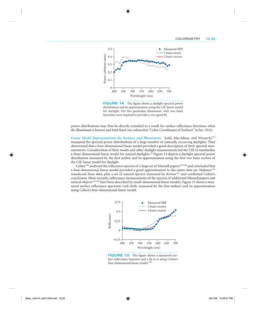
COLORIMETRY 10.33
power distributions may thus be directly extended to a result for surface reflectance functions when the illuminant is known and held fixed (see subsection “Color Coordinates of Surfaces” in Sec. 10.6).
Linear Model Representations for Surfaces and Illuminants Judd, MacAdam, and Wyszecki137 measured the spectral power distributions of a large number of naturally occurring daylights. They determined that a four-dimensional linear model provided a good description of their spectral mea-surements. Consideration of their results and other daylight measurements led the CIE to standardize a three-dimensional linear model for natural daylights.10 Figure 14 depicts a daylight spectral power distribution measured by the first author and its approximation using the first two basis vectors of the CIE linear model for daylight.
Cohen138 analyzed the reflectance spectra of a large set of Munsell papers139,140 and concluded that a four-dimensional linear model provided a good approximation to the entire data set. Maloney141
reanalyzed these data, plus a set of natural spectra measured by Krinov142 and confirmed Cohen’s conclusion. More recently, reflectance measurements of the spectra of additional Munsell papers and natural objects143,144 have been described by small-dimensional linear models. Figure 15 shows a mea-sured surface reflectance spectrum (red cloth, measured by the first author) and its approximation using Cohen’s four-dimensional linear model.
Measured SPD
2 basis vectors
0
0.1
0.2
0.3
0.4
0.5
400 450 500 550 600 650 700
1 basis vector
Pow
er (
arbi
trar
y u
nit
s)
Wavelength (nm)
FIGURE 14 The figure shows a daylight spectral power distribution and its approximation using the CIE linear model for daylight. For this particular illuminant, only two basis functions were required to provide a very good fit.
−0.25
0
0.25
0.5
0.75
400 450 500 550 600 650 700
Measured SRF2 basis vectors4 basis vectors
Ref
lect
ance
Wavelength (nm)
FIGURE 15 The figure shows a measured sur-face reflectance function and a fit to it using Cohen’s four-dimensional linear model.138
Bass_v3ch10_p001-056.indd 10.33Bass_v3ch10_p001-056.indd 10.33 8/21/09 12:49:57 PM8/21/09 12:49:57 PM
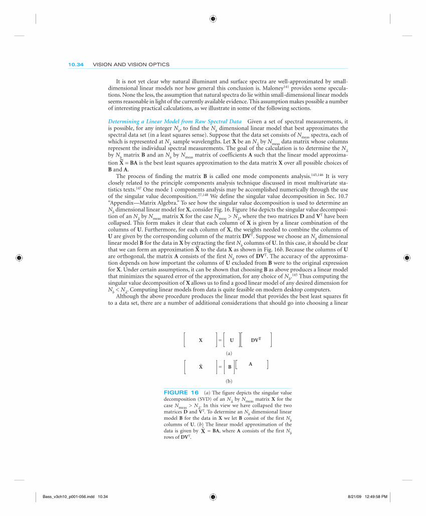
10.34 VISION AND VISION OPTICS
It is not yet clear why natural illuminant and surface spectra are well-approximated by small-dimensional linear models nor how general this conclusion is. Maloney141 provides some specula-tions. None the less, the assumption that natural spectra do lie within small-dimensional linear models seems reasonable in light of the currently available evidence. This assumption makes possible a number of interesting practical calculations, as we illustrate in some of the following sections.
Determining a Linear Model from Raw Spectral Data Given a set of spectral measurements, it is possible, for any integer Nb, to find the Nb dimensional linear model that best approximates the spectral data set (in a least squares sense). Suppose that the data set consists of Nmeas spectra, each of which is represented at Nl sample wavelengths. Let X be an Nl by Nmeas data matrix whose columns represent the individual spectral measurements. The goal of the calculation is to determine the Nl by Nb matrix B and an Nb by Nmeas matrix of coefficients A such that the linear model approxima-
tion X~
= BA is the best least squares approximation to the data matrix X over all possible choices of B and A.
The process of finding the matrix B is called one mode components analysis.145,146 It is very closely related to the principle components analysis technique discussed in most multivariate sta-tistics texts.147 One mode 1 components analysis may be accomplished numerically through the use of the singular value decomposition.27,148 We define the singular value decomposition in Sec. 10.7 “Appendix—Matrix Algebra.” To see how the singular value decomposition is used to determine an Nb dimensional linear model for X, consider Fig. 16. Figure 16a depicts the singular value decomposi-tion of an Nl by Nmeas matrix X for the case Nmeas > Nl, where the two matrices D and VT have been collapsed. This form makes it clear that each column of X is given by a linear combination of the columns of U. Furthermore, for each column of X, the weights needed to combine the columns of U are given by the corresponding column of the matrix DVT. Suppose we choose an Nb dimensional linear model B for the data in X by extracting the first Nb columns of U. In this case, it should be clear that we can form an approximation X
~ to the data X as shown in Fig. 16b. Because the columns of U
are orthogonal, the matrix A consists of the first Nb rows of DVT. The accuracy of the approxima-tion depends on how important the columns of U excluded from B were to the original expression for X. Under certain assumptions, it can be shown that choosing B as above produces a linear model that minimizes the squared error of the approximation, for any choice of Nb.
145 Thus computing the singular value decomposition of X allows us to find a good linear model of any desired dimension for Nb < Nl. Computing linear models from data is quite feasible on modern desktop computers.
Although the above procedure produces the linear model that provides the best least squares fit to a data set, there are a number of additional considerations that should go into choosing a linear
X = U DVT
X = BA
(a)
(b)
FIGURE 16 (a) The figure depicts the singular value decomposition (SVD) of an Nl by Nmeas matrix X for the case Nmeas > Nl. In this view we have collapsed the two matrices D and VT. To determine an Nb dimensional linear model B for the data in X we let B consist of the first Nb columns of U. (b) The linear model approximation of the data is given by X̂ = BA, where A consists of the first Nb rows of DVT.
Bass_v3ch10_p001-056.indd 10.34Bass_v3ch10_p001-056.indd 10.34 8/21/09 12:49:58 PM8/21/09 12:49:58 PM
COLORIMETRY 10.35
model. First, we note that the choice of linear model is not unique. Any nonsingular linear combina-tion of the columns of B will produce a linear model that provides an equally good account of the data. Second, the least squares error measure gives more weight to spectra with large amplitudes. In the case of surface spectra, this means that the more reflective surfaces will tend to drive the choice of basis vectors. In the case of illuminants, the more intense illuminants will tend to drive the choice. To avoid this weighting, the measured spectra are sometimes normalized to unit length before perform-ing the singular value decomposition. The normalization equalizes the effect of the relative shape of each spectrum in the data set.141 Third, it is sometimes desired to find a linear model that best describes the variation of a data set around its mean. To do this, the mean of the data set should be subtracted before performing the singular value decomposition. When the mean of the data is subtracted, one mode components analysis is identical to principle components analysis. Finally, there are circumstances where the linear model will be used not to approximate spectra but rather to approximate some other quantity (e.g., color coordinates) that depend on the spectra. In this case, more general techniques, closely related to those discussed here, may be used.149
Approximating a Spectrum with Respect to a Linear Model Given an Nb dimensional linear model B, it is straightforward to find the representation of any spectrum with respect to the linear model. Let X be a matrix representing the spectra of functions to be approximated. These spectra do not need to be members of the data set that was used to determine the linear model. To find the matrix of coefficients A such that X
~ = BA best approximates X we use simple linear regression.
Regression routines to solve this problem are provided as part of any standard matrix algebra software package.
Digital Image Representations If in a given application illuminants and surfaces may be repre-sented with respect to small-dimensional linear models, then it becomes feasible to use point-by-point representations of these quantities in digital image processing. In typical color image processing, the image data at each point are represented by three numbers at each location. These numbers are generally tristimulus values in some color space. In calibrated systems, side information about the color-matching functions or primary spectral power distributions that define the color space is available to interpret the tristimulus values. It is straightforward to generalize this notion of color images by allowing the images to contain Nb numbers at each point and allowing these numbers to represent quantities other than tristimulus values.7 For example, in representing the image produced by a printer, it might be advantageous to represent the surface reflectance at each location.150 If the gamut of printed reflectances can be represented within a small-dimensional linear model, then rep-resenting the surface reflectance functions with respect to this model would not require much more storage than a traditional color image.7 The basis functions for the linear model only need be rep-resented once, not at each location. But by representing reflectances rather than tristimulus values, it becomes possible to compute what the tristimulus values reflected from the printed image would be under any illumination. We illustrate the calculation in the next section. Because of the problem of metamerism (see subsection “Computing the Reflected Light”), this calculation is not possible if only the tristimulus values are represented in the digital image. To avoid this limitation, hyperspectral images record full spectra at each image location.151–153
Simulation of Illuminated Surfaces Consider the problem of producing a signal on a monitor that has the same tristimulus values as a surface under a variety of different illuminants. The solution to this problem is straightforward and is useful in a number of applications. These include render-ing digitally archived paintings,154,155 generating stimuli for use in psychophysics,156 and producing photorealistic computer-generated imagery.17 We show the calculation for the data at a single image location. Let a be a representation of the surface reflectance with respect to an Nb dimensional linear model B. Let E represent the illuminant spectral power distribution in diagonal matrix form. Let T represent the color-matching functions for a human observer, and P represent the primary phos-phor spectral power distributions for the monitor on which the surface will be rendered. We wish to determine tristimulus values t with respect to the monitor primaries so that the light emitted from the monitor will appear identical to the light reflected from the simulated surface under the
Bass_v3ch10_p001-056.indd 10.35Bass_v3ch10_p001-056.indd 10.35 8/21/09 12:49:58 PM8/21/09 12:49:58 PM
10.36 VISION AND VISION OPTICS
simulated illuminant. From Eqs. (13) (cast as s = Ba), (34), (29), and (30) we can write directly the desired rendering equation
t = [(TP)–1(TE)B]a (35)
The rendering matrix [(TP)–1 (TE)B] has dimensions 3 by Nb and maps the surface weights directly to monitor tristimulus values. It is quite general, in that we may use it for any calibrated monitor and any choice of linear models. It does not depend on the particular surface being rendered and may be computed once for an entire image. Because the rendering matrix is of small dimension, ren-dering of this sort is feasible, even for very large images. As discussed in subsection “Transformations between Color Spaces” in Sec. 10.5, it may be possible to determine the matrix MT,P = (TP)–1 directly. A similar shortcut is possible for the matrix (TE)B. Each column of this matrix is the tristimulus values of one linear model basis vector under the illuminant specified by the matrix E.
Color Coordinates of Surfaces Our discussion thus far has emphasized describing the color coordi-nates of lights. In many applications of colorimetry, it is desirable to describe the color properties of reflective objects. One efficient way to do this, as described above, is to use linear models to describe the full surface reflectance functions. Another possibility is to specify the color coordinates of the light reflected from the surface under standard illumination. This method allows the assignment of tristimulus values to surfaces in an orderly fashion.
The CIE has standardized several illuminant spectral power distributions that may be used for this purpose (see the next section). Using the procedures defined above, one can begin with the spectral power distribution of the illuminant and the surface reflectance function and from there calculate the desired color-matching coordinates.
The relative size of the tristimulus values assigned to a surface depend on its spectral reflectance function and on the illuminant chosen for specification. To factor the intensity of the illuminant out of the surface representation, the CIE specified a normalization of the color coordinates for use with 1931 XYZ tristimulus values. This normalization consists of multiplying the computed tristimulus values by the quantity 100/Y0, where Y0 is the Y tristimulus value for the illuminant.
The tristimulus values of a surface provide enough information to match the surface when it is viewed under the illuminant used to compute those coordinates. It is important to bear in mind that two surfaces that have the same tristimulus values under one illuminant do not necessarily share the same tristimulus values under another illuminant. A more complete description can be generated using the linear model approach described above.
Standard Sources of Illumination The CIE has standardized a number of illuminant spectral power distributions.157 These were designed to be typical of various common viewing conditions and are useful as specific choices of illumination when the illuminant cannot be measured directly. CIE Illuminant A is designed to be representative of tungsten-filament illumination. CIE Illuminant D65 is designed to be representative of average daylight. Other CIE standard daylight illuminants may be computed using the CIE principle components of daylight as basis vectors and the formulas specified by the CIE.10 Spectra representative of fluorescent lamps and other artificial sources are also available.8,10
Metamerism
Recovering Spectral Power Distributions from Tristimulus Values It is not possible in general to recover a spectral power distribution from its tristimulus values. If some prior information about the spectral power distribution of the color signal is available, however, then recovery may be possible. Such recovery is of most interest in applications where direct spectral measurements are not possible and where knowing the full spectrum is important. For example, the effect of lens chromatic aberra-tions on cone quantal absorption rates depends on the full spectral power distribution.110
Suppose the spectral power distribution of interest is known to lie within a three-dimensional linear model. We may write b = Ba, where the basis matrix B has dimensions Nl by 3. Let t be the
Bass_v3ch10_p001-056.indd 10.36Bass_v3ch10_p001-056.indd 10.36 8/21/09 12:49:58 PM8/21/09 12:49:58 PM

COLORIMETRY 10.37
tristimulus values of the light with respect to a set of color-matching functions T. We can conclude that a = (TB )
–1 t, which implies
b = B(TB )–1t (36)
When we do not have a prior constraint that the signal belongs to a three-dimensional linear model, we may still be able to place some linear model constraint, of dimension higher than three, on the spectral power distribution. For example, when we know that the signal was produced by the reflection of daylight from a natural object, it is reasonable to assume that the color signal lies within a linear model of dimension that may be as low as nine.158 In this case, we can still write b = Ba, but we cannot apply Eq. (36) directly because the matrix (TB) will be singular. To deal with this prob-lem, we can choose a reduced linear model with only three dimensions. We then proceed as outlined above, but substitute the reduced model for the true model. This will lead to an estimate for the actual spectral power distribution b. If the reduced linear model provides a reasonable approximation to b, the estimation error may be quite small. The estimate will have the property that it is a metamer of b. The techniques described above for finding linear model approximations may be used to choose an appropriate reduced model.
Finding Metamers of a Light It is often of interest to find metamers of a light. We discuss two approaches here. Wyszecki and Stiles8 treat the problem in considerable detail.
Using a linear model If we choose any three-dimensional linear model we can combine Eq. (36) with the fact the fact that t = Tb [Eq. (20)] to compute a pair of metameric spectral power distribu-
tions b and b̂
ˆ ˆ ˆb B(TB) Tb–1= (37)
Each choice of B̂ will lead to a different metamer. Figure 17 shows a number of metameric spectral power distributions generated in this fashion.
0
1
2
3
4
5
400 450 500 550 600 650 700
DaylightMonitorFundamental
Pow
er
Wavelength (nm)
FIGURE 17 The figure shows three metameric color signals with respect to the CIE 1931 standard observer. The three metamers were computed using Eq. (37). The initial spectral power distribution b (not shown) was an equal energy spectrum. Three separate linear models were used: one that describes natural daylights, one typical of monitor phosphor spectral power distributions, and one that provides Cohen’s “fundamental metamer.”207
Bass_v3ch10_p001-056.indd 10.37Bass_v3ch10_p001-056.indd 10.37 8/21/09 12:49:59 PM8/21/09 12:49:59 PM
10.38 VISION AND VISION OPTICS
Metameric blacks Another approach to generating metamers is to note that there will be some spectral power distributions b0 that have the property Tb0 = 0. Wyszecki referred to such distributions as metameric blacks, since they have the same tristimulus values as no light at all.159 Grassmann’s laws imply that adding a metameric black b0 to any light b yields a metamer of b. Given a linear model B with dimension greater than three it is possible to find a second linear model B0 such that (a) all lights that lie in B0 also lie in B and (b) all lights in B0 are metameric blacks. We determine B0 by finding a linear model for the null space of the matrix TB. The null space of a matrix consists of all vectors that are mapped to 0 by the matrix. Finding a basis for the null space of a matrix is a standard operation in numerical matrix algebra. If we have a set of basis vectors N0 for the null space of TB, we can form B0 = BN0. This technique provides a way to generate a large list of metamers for any given light b. We choose a set of weights a at random and construct b0 = B0a. We then add b0 to b to form a metamer. To generate more metamers, we simply repeat with new choices of weight vector a.
Surface and Illuminant Metamerism The formal similarity between Eq. (20) (which gives the relation between spectral power distributions and tristimulus values) and Eq. (34) (which gives the relation between surface reflectance functions and tristimulus values when the illuminant is known) makes it clear that our discussion of metamerism can be applied to surface reflectance spectra. Two physically different surfaces will appear identical if the tristimulus values of the light reflected from them is identical. This fact can be used to good purpose in some color reproduction applications. Suppose that we have a sample surface or textile whose color we wish to reproduce. It may be that we are not able to reproduce the sample’s surface reflectance function exactly because of various limitations in the available color reproduction technology. If we know the illuminant under which the reproduction will be viewed, we may be able to determine a reproducible reflectance function that is metameric to that of the desired sample. This will give us a sample whose color appearance is as desired. Applications of this sort make heavy use of the methods described earlier to determine metamers.
But what if the illuminant is not known or if it is known to vary? In this case there is an additional richness to the topic of determining metamers. We can pose the problem of finding surface reflec-tance functions that will be metameric to a desired reflectance under multiple specified illuminants or under all of the illuminants within some linear model. The general methods developed here have been extended to analyze this case.158,160 Similar issues arise in lighting design, where we desire to produce an artificial light whose color-rendering properties match those of a specified light (such as natural daylight). When wavelength by wavelength matching of the spectra is not feasible, it may still be possible to find a spectrum so that the light reflected from surfaces within a linear model is identi-cal for the two light sources. Because of the symmetric role of illuminants and surfaces in reflection, this problem may be treated by the same methods as used for surface reproduction.
Color Cameras and Other Visual Systems
We have treated colorimetry from the point of view of specifying the spectral information avail-able to a human observer. We have developed our treatment, however, in such a way that it may be applied to handle other visual systems. Suppose that we wish to define color coordinates with respect to some arbitrary visual system with Ndevice photosensors. This visual system might be an artificial system based on a color camera or scanner, a nonhuman biological visual system, or the visual system of a color anomalous human observer. We assume that the sensitivities of the visual system’s photo-sensors are known up to a linear transformation. Let Tdevice be an Ndevice by Nl matrix whose entries are the sensitivities of each of the device’s sensors at each sample wavelength. We can compute the responses of these sensors to any light b. Let tdevice be a vector containing the responses of each sensor type to the light. Then we have tdevice = Tdevice b. We may use tdevice as the device color coordinates of b.
Transformation between Color Coordinates of Different Visual Systems Suppose that we have two different visual systems and we wish to transform between the color coordinates of each.
Bass_v3ch10_p001-056.indd 10.38Bass_v3ch10_p001-056.indd 10.38 8/21/09 12:49:59 PM8/21/09 12:49:59 PM
COLORIMETRY 10.39
A typical example might be trying to compute the CIE 1931 XYZ tristimulus values of a light from the responses of a color camera. Let Ns be the number of source sensors, with sensitivities specified by Ts. Similarly, let Nd by the number of destination sensors with sensitivities specified by Td. For any light b we know that the source device color coordinates are given by ts = Tsb and the destina-tion device color coordinates td = Tdb. We would like to transform between ts and td without direct knowledge of b.
If we can find an Nd by Ns matrix M such that Td = MTs then it is easy to show that the matrix M may be used to compute the destination device color coordinates from the source device color coor-dinates through td = Mts. We have already considered this case (in a less general form) in subsection “Transformations between Color Spaces.” The extension here is that we allow the possibility that the dimensions of the two color coordinate systems differ. When a linear transformation between Ts and Td exists, it can be found by standard regression methods.
Horn demonstrated that when no exact linear transformation between Ts and Td exists, it is not in general possible to transform between the two sets of color coordinates.4 The reason for this is that there will always exist a pair of lights that have the same color coordinates for the source device but different color coordinates for the destination device. The transformation will therefore be incorrect for at least one member of this pair. When no exact linear transformation exists, it is still possible to make an approximate transformation. One approach is to use linear regression to find the best linear transformation M between the two sets of color-matching functions in a least squares sense. This transformation is then applied to the source color coordinates as if it were exact.4 Although this is an approximation, in many cases the results will be acceptable. In the absence of prior information about the spectral power distribution of the original light b, it is a sensible approach.
A second possibility is to use prior constraints on the spectral power distribution of the light to guide the transformation.22 Suppose that we know that the light is constrained to lie within an Nb dimensional linear model B. Then we can find the best linear transformation M between the two matrices TsB and TdB. This transformation may then be used to transform the source color coordi-nates to the destination color coordinates. It is easy to show that the transformation will be exact if TdB = MTsB. Otherwise it is a reasonable approximation that takes the linear model constraint into account.
A number of recent papers present more elaborated methods for color correction.161–163
Computational Color Constancy An interesting application is the problem of estimating surface reflectance functions from color coordinates. This problem is of interest for two reasons. First, it appears that human color vision makes some attempt to perform this estimation, so that our per-cept of color is more closely associated with object surface properties than with the proximal prop-erties of the light reaching the eye. Second, an artificial system that could estimate surface properties would have an important cue to aid object recognition. In the case where the illuminant is known, the problem of estimating surface reflectance properties is the same as the problem of estimating the color signal, because the illuminant spectral power distribution can simply be incorporated into the sensor sensitivities. In this case the methods outlined in the preceding section for estimating color signal spectral properties can be used.
The more interesting case is where both the illuminant and the surface reflectance are unknown. In this case, the problem is more difficult. Considerable insight has been gained by applying lin-ear model constraints to both the surface and illuminant spectral power distributions. A number of approaches have been developed for recovering surface reflectance functions or otherwise achieving color constancy.158,164–172 Each approach differs (1) in the additional assumptions that are made about the properties of the image and (2) in the sophistication of the model of illuminant surface interac-tion and scene geometry used. A thorough review of all of these methods is beyond the scope of this chapter. It is instructive, however, to review one of the simpler methods, that of Buchsbaum.165 See Ebner173 for a discussion of many current algorithms.
Buchsbaum assumed that in any given scene, the average reflectance function of the surfaces in the scene is known. This is commonly called the “gray world” assumption. He also assumed that the illuminant was diffuse and constant across the scene and that the illuminants and surfaces in the scene are described by linear models with the same dimensionality as the number of sensors.
Bass_v3ch10_p001-056.indd 10.39Bass_v3ch10_p001-056.indd 10.39 8/21/09 12:49:59 PM8/21/09 12:49:59 PM
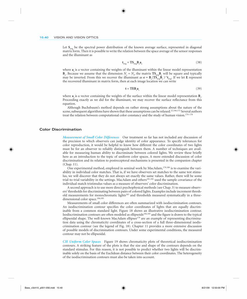
10.40 VISION AND VISION OPTICS
Let Savg be the spectral power distribution of the known average surface, represented in diagonal matrix form. Then it is possible to write the relation between the space average of the sensor responses and the illuminant as
tavg = TSavgBeae (38)
where ae is a vector containing the weights of the illuminant within the linear model representation Be. Because we assume that the dimension Ne = Nt, the matrix TSavgBe will be square and typically may be inverted. From this we recover the illuminant as e = Be(TSavgBe )
–1tavg. If we let E represent the recovered illuminant in matrix form, then at each image location we can write
t = TEBsas (39)
where as is a vector containing the weights of the surface within the linear model representation Bs. Proceeding exactly as we did for the illuminant, we may recover the surface reflectance from this equation.
Although Buchsbaum’s method depends on rather strong assumptions about the nature of the scene, subsequent algorithms have shown that these assumptions can be relaxed.22,166,172 Several authors treat the relation between computational color constancy and the study of human vision.174–178
Color Discrimination
Measurement of Small Color Differences Our treatment so far has not included any discussion of the precision to which observers can judge identity of color appearance. To specify tolerances for color reproduction, it would be helpful to know how different the color coordinates of two lights must be for an observer to reliably distinguish between them. A number of techniques are avail-able for measuring human ability to discriminate between colored lights. We review these briefly here as an introduction to the topic of uniform color spaces. A more extended discussion of color discrimination and its relation to postreceptoral mechanisms is presented in the companion chapter (Chap. 11).
One experimental method, employed in seminal work by MacAdam,179,180 is to examine the vari-ability in individual color matches. That is, if we have observers set matches to the same test stimu-lus, we will discover that they do not always set exactly the same values. Rather, there will be some trial-to-trial variability in the settings. MacAdam and others181,182 used the sample covariance of the individual match tristimulus values as a measure of observers’ color discrimination.
A second approach is to use more direct psychophysical methods (see Chap. 3) to measure observ-ers’ thresholds for discriminating between pairs of colored lights. Examples include increment thresh-old measurements for monochromatic lights183 and thresholds measured systematically in a three-dimensional color space.184,185
Measurements of small color differences are often summarized with isodiscrimination contours. An isodiscrimination contour specifies the color coordinates of lights that are equally discrim-inable from a common standard light. Figure 18 shows an illustrative isodiscrimination contour. Isodiscrimination contours are often modeled as ellipsoids184,185 and the figure is drawn to the typical ellipsoidal shape. The well-known MacAdam ellipses179 are an example of representing discrimina-tion data using the chromaticity coordinates of a cross-section of a full three-dimensional isodis-crimination contour (see the legend of Fig. 18). Chapter 11 provides a more extensive discussion of possible models of discrimination contours. Under some experimental conditions, the measured contour may not be ellipsoidal.
CIE Uniform Color Spaces Figure 19 shows chromaticity plots of theoretical isodiscrimination contours. A striking feature of the plots is that the size and shape of the contours depends on the standard stimulus. For this reason, it is not possible to predict whether two lights will be discrim-inable solely on the basis of the Euclidean distance between their color coordinates. The heterogeneity of the isodiscrimination contours must also be taken into account.
Bass_v3ch10_p001-056.indd 10.40Bass_v3ch10_p001-056.indd 10.40 8/21/09 12:50:00 PM8/21/09 12:50:00 PM
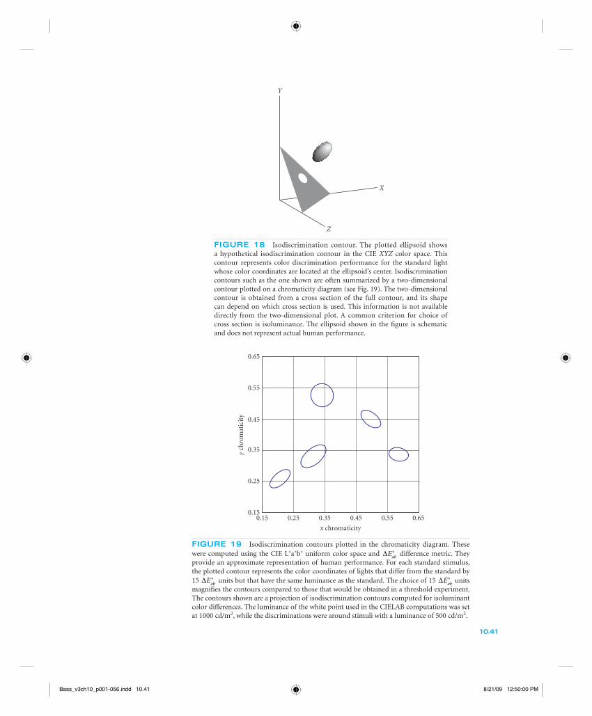
X
Y
Z
FIGURE 18 Isodiscrimination contour. The plotted ellipsoid shows a hypothetical isodiscrimination contour in the CIE XYZ color space. This contour represents color discrimination performance for the standard light whose color coordinates are located at the ellipsoid’s center. Isodiscrimination contours such as the one shown are often summarized by a two-dimensional contour plotted on a chromaticity diagram (see Fig. 19). The two-dimensional contour is obtained from a cross section of the full contour, and its shape can depend on which cross section is used. This information is not available directly from the two-dimensional plot. A common criterion for choice of cross section is isoluminance. The ellipsoid shown in the figure is schematic and does not represent actual human performance.
0.65
0.55
0.45
0.35
0.25
0.150.15 0.25 0.35 0.45 0.55 0.65
x chromaticity
y ch
rom
atic
ity
FIGURE 19 Isodiscrimination contours plotted in the chromaticity diagram. These were computed using the CIE L∗a∗b∗ uniform color space and ΔEab
∗ difference metric. They provide an approximate representation of human performance. For each standard stimulus, the plotted contour represents the color coordinates of lights that differ from the standard by 15 ΔEab
∗ units but that have the same luminance as the standard. The choice of 15 ΔEab∗ units
magnifies the contours compared to those that would be obtained in a threshold experiment. The contours shown are a projection of isodiscrimination contours computed for isoluminant color differences. The luminance of the white point used in the CIELAB computations was set at 1000 cd/m2, while the discriminations were around stimuli with a luminance of 500 cd/m2.
10.41
Bass_v3ch10_p001-056.indd 10.41Bass_v3ch10_p001-056.indd 10.41 8/21/09 12:50:00 PM8/21/09 12:50:00 PM
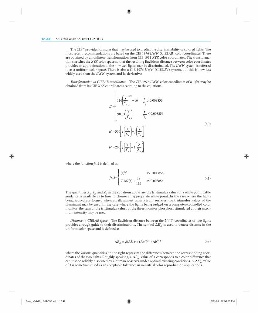
10.42 VISION AND VISION OPTICS
The CIE10 provides formulas that may be used to predict the discriminability of colored lights. The most recent recommendations are based on the CIE 1976 L∗a∗b∗ (CIELAB) color coordinates. These are obtained by a nonlinear transformation from CIE 1931 XYZ color coordinates. The transforma-tion stretches the XYZ color space so that the resulting Euclidean distance between color coordinates provides an approximation to the how well lights may be discriminated. The L∗a∗b∗ system is referred to as a uniform color space. There is also a CIE 1976 L∗u∗v∗ (CIELUV) system, but this is now less widely used than the L∗a∗b∗ system and its derivatives.
Transformation to CIELAB coordinates The CIE 1976 L∗a∗b∗ color coordinates of a light may be obtained from its CIE XYZ coordinates according to the equations
Ln n
n
∗ =
⎛
⎝⎜
⎞
⎠⎟ − >
⎛
⎝⎜
⎞
⎠⎟
116 16 0 008856
903 3
1 3YY
YY
YY
/
.
.YYY
XX
YY
n
n n
a f f
≤
⎧
⎨
⎪⎪⎪
⎩
⎪⎪⎪
=⎛
⎝⎜
⎞
⎠⎟−
⎛
⎝⎜
⎞∗
0 008856
500
.
⎠⎠⎟
⎡
⎣⎢⎢
⎤
⎦⎥⎥
=⎛
⎝⎜
⎞
⎠⎟−
⎛
⎝⎜
⎞
⎠⎟
⎡
⎣⎢⎢
⎤
⎦⎥⎥
∗b f fn n
200YY
ZZ
(40)
where the function f (s) is defined as
f ss s
s s( )
( ) .
. ( ) .
/
=>
+ ≤
1 3 0 008856
7 78716
1160 008856
⎧⎧
⎨⎪
⎩⎪
(41)
The quantities Xn, Yn, and Zn in the equations above are the tristimulus values of a white point. Little guidance is available as to how to choose an appropriate white point. In the case where the lights being judged are formed when an illuminant reflects from surfaces, the tristimulus values of the illuminant may be used. In the case where the lights being judged on a computer-controlled color monitor, the sum of the tristimulus values of the three monitor phosphors stimulated at their maxi-mum intensity may be used.
Distance in CIELAB space The Euclidean distance between the L∗a∗b∗ coordinates of two lights provides a rough guide to their discriminability. The symbol ΔEab
∗ is used to denote distance in the uniform color space and is defined as
Δ Δ Δ ΔE L a bab
∗ ∗ ∗ ∗= + +( ) ( ) ( )2 2 2 (42)
where the various quantities on the right represent the differences between the corresponding coor-dinates of the two lights. Roughly speaking, a ΔEab
∗ value of 1 corresponds to a color difference that can just be reliably discerned by a human observer under optimal viewing conditions. A ΔEab
∗ value of 3 is sometimes used as an acceptable tolerance in industrial color reproduction applications.
Bass_v3ch10_p001-056.indd 10.42Bass_v3ch10_p001-056.indd 10.42 8/21/09 12:50:00 PM8/21/09 12:50:00 PM
COLORIMETRY 10.43
The CIE color difference measure ΔEab∗ provides only an approximate guide to the discriminability
between two lights. There are a number of reasons why this is so. The first is that the relatively simple nonlinear transformation between CIE XYZ and CIE L∗a∗b∗ coordinates does not completely capture the empirical data on color discrimination between two samples. In part this is because the formulae were designed to predict not only discrimination data but also certain suprathreshold judgments of color appearance.186 Second, color discrimination thresholds depend heavily on factors other than the tristimulus values. These factors include the adapted state of the observer,183 the spatial and tem-poral structure of the stimulus,187–189
and the task demands placed on the observer.190–193 Therefore, the complete specification of a uniform color space must incorporate these factors. The CIE has now recommended a more involved method of computing small color differences from the CIE L∗a∗b∗ coordinates that attempts to provide better prediction of small color differences.10,194 The resultant computed difference is referred to as ΔE00. The details of the computation of ΔE00 are provided and discussed in a CIE technical report.194 The reader considering using ΔE00 is encouraged to study Wyszecki and Stiles’s8(pp. 584–586) insightful discussion of color vision models.
Effect of Errors in Color-Matching Functions
Given that there is some variation between different standard estimates of color-matching functions, between the color-matching functions of different individuals, and between the color-matching functions that mediate performance for different viewing conditions, it is of interest to determine whether the magnitude of this variation is of practical importance. There is probably no general method for making this determination, but here we outline one approach.
Consider the case of rendering a set of illuminated surfaces on a color monitor. If we know the spectral power distribution of the monitor’s phosphors, it is possible to compute the appropriate weights on the monitor phosphors to produce a light metameric to each illuminated surface. The computed weights will depend on the choice of color-matching functions. Once we know the weights, however, we can find the L∗a∗b∗ coordinates of the emitted light. This suggests the following method to estimate the effect of differences in color-matching functions. First we compute the L∗a∗b∗ coor-dinates of surfaces rendered using the first set of color-matching functions. Then we compute the corresponding coordinates when the surfaces are rendered using the second set of color-matching functions. Finally, we compute the ΔEab
∗ difference between corresponding sets of coordinates. If the ΔEab
∗ are large, then the differences between the color-matching functions are important for the rendering application.
We have performed this calculation for a set of 462 measured surfaces139,140 rendered under CIE Illuminant D65. The two sets of color-matching functions used were the 1931 CIE XYZ color-matching functions and the Judd-Vos modified XYZ color-matching functions. The monitor phosphor spec-tral power distributions were measured by the first author. The results are shown in Fig. 20. The plot shows a histogram of the differences. The median difference is 1.2 units. This difference is quite close to discrimination threshold and for many applications, the differences between the two sets of color-matching functions will probably not be of great consequence.
Brightness Matching and Photometry
The foundation of colorimetry is the human observer’s ability to judge identity of color appearance. It is sometimes of interest to compare certain perceptual attributes of lights that do not, as a whole, appear identical. In particular, there has been a great deal of interest in developing formulas that pre-dict when two lights with different relative spectral power distributions will appear equally bright. Colorimetry provides a partial answer to this question, since two lights that match in appearance must appear equally bright. Intuitively, however, it seems that it should be possible to set the relative intensities of any two lights so that they match in brightness.
In a heterochromatic brightness matching experiment, observers are asked to scale the intensity of a matching light until its brightness matches that of an experimentally controlled test light. Although
Bass_v3ch10_p001-056.indd 10.43Bass_v3ch10_p001-056.indd 10.43 8/21/09 12:50:00 PM8/21/09 12:50:00 PM
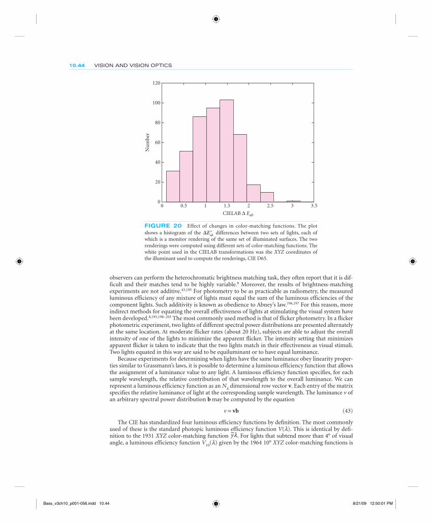
10.44 VISION AND VISION OPTICS
observers can perform the heterochromatic brightness matching task, they often report that it is dif-ficult and their matches tend to be highly variable.8 Moreover, the results of brightness-matching experiments are not additive.43,195 For photometry to be as practicable as radiometry, the measured luminous efficiency of any mixture of lights must equal the sum of the luminous efficiencies of the component lights. Such additivity is known as obedience to Abney’s law.196,197 For this reason, more indirect methods for equating the overall effectiveness of lights at stimulating the visual system have been developed.8,195,198–203 The most commonly used method is that of flicker photometry. In a flicker photometric experiment, two lights of different spectral power distributions are presented alternately at the same location. At moderate flicker rates (about 20 Hz), subjects are able to adjust the overall intensity of one of the lights to minimize the apparent flicker. The intensity setting that minimizes apparent flicker is taken to indicate that the two lights match in their effectiveness as visual stimuli. Two lights equated in this way are said to be equiluminant or to have equal luminance.
Because experiments for determining when lights have the same luminance obey linearity proper-ties similar to Grassmann’s laws, it is possible to determine a luminous efficiency function that allows the assignment of a luminance value to any light. A luminous efficiency function specifies, for each sample wavelength, the relative contribution of that wavelength to the overall luminance. We can represent a luminous efficiency function as an Nl dimensional row vector v. Each entry of the matrix specifies the relative luminance of light at the corresponding sample wavelength. The luminance v of an arbitrary spectral power distribution b may be computed by the equation
v = vb (43)
The CIE has standardized four luminous efficiency functions by definition. The most commonly used of these is the standard photopic luminous efficiency function V(l). This is identical by defi-nition to the 1931 XYZ color-matching function yλ. For lights that subtend more than 4° of visual angle, a luminous efficiency function V10(l) given by the 1964 10° XYZ color-matching functions is
120
100
80
60N
um
ber
40
20
00 0.5 1 1.5 2 2.5 3 3.5
CIELAB Δ Eab
FIGURE 20 Effect of changes in color-matching functions. The plot shows a histogram of the ΔEab
∗ differences between two sets of lights, each of which is a monitor rendering of the same set of illuminated surfaces. The two renderings were computed using different sets of color-matching functions. The white point used in the CIELAB transformations was the XYZ coordinates of the illuminant used to compute the renderings, CIE D65.
Bass_v3ch10_p001-056.indd 10.44Bass_v3ch10_p001-056.indd 10.44 8/21/09 12:50:01 PM8/21/09 12:50:01 PM
COLORIMETRY 10.45
preferred. More recently, the Judd-Vos modified color matching function has been made a supple-mental standard.204 A final standard luminous efficiency function is available for use at low light levels when the rods are the primary functioning photoreceptors. A new luminous efficiency function will be incorporated into the new CIE proposal for a set of physiologically relevant color-matching func-tions. The notation Vl or V(l) is often used in the literature to denote luminous efficiency functions. Note that Eq. (43) allows the computation of luminance in arbitrary units. Ref. 8 discusses standard measurement units for luminance.
It is important to note that luminance is a construct derived from flicker photometric and related experiments. As such, it does not directly predict when two lights will be judged to have the same brightness. The relation between luminance and brightness is quite complicated.8,205
It is also worth noting that there is considerable individual variation in flicker photometric judg-ments, even among color-normal observers. For this reason, it is a common practice in psychophysi-cal experiments to use flicker photometry to determine isoluminant stimuli for individual subjects with the stimuli of interest.
10.7 APPENDIX—MATRIX ALGEBRA
This appendix provides a brief introduction to matrix algebra. The development emphasizes the aspects of matrix algebra that are used in this chapter and is somewhat idiosyncratic. In addition, we do not prove any of the results we state. Rather, our intention is to provide the reader unfamiliar with matrix algebra with enough information to make this chapter self-contained.
Basic Notions
Vectors and Matrices A vector is a list of numbers. We use lowercase bold letters to represent vec-tors. We use single subscripts to identify the individual entries of a vector. The entry ai refers to the ith number in a. We call the total number of entries in a vector its dimension.
A matrix is an array of numbers. We use uppercase bold letters to represent matrices. We use dual subscripts to identify the individual entries of a matrix. The entry aij refers to the number in the ith row and jth column of A. We sometimes refer to this as the ijth entry of A. We call the number of rows in a matrix its row dimension. We call the number of columns in a matrix its column dimension. We generally use the symbol N to denote dimensions.
Vectors are a special case of matrices where either the row or the column dimension is 1. A matrix with a single column is often called a column vector. A matrix with a single row is often called a row vector. By convention, all vectors used in this chapter should be understood to be column vectors unless explicitly noted otherwise.
It is often convenient to think of a matrix as being composed of vectors. For example, if a matrix has dimensions Nr by Nc, then we may think of the matrix as consisting of Nc column vectors, each of which has dimension Nr.
Addition and Multiplication A vector may be multiplied by a number. We call this scalar mul-tiplication. Scalar multiplication is accomplished by multiplying each entry of the vector by the number. If a is a vector and b is a number, then b = ab = ba is a vector whose entries are given by cj = baj.
Two vectors may be added together if they have the same dimension. We call this vector addition. Vector addition is accomplished through entry-by-entry addition. If a and b are vectors with the same dimension, the entries of c = a + b are given by cj = aj + bj.
Two matrices may be added if they have the same row and column dimensions. We call this matrix addition. Matrix addition is also defined as entry by entry addition. Thus if A and B are matrices with the same dimension, the entries of C = A + B are given by cij = aij + bij. Vector addition is a special case of matrix addition.
Bass_v3ch10_p001-056.indd 10.45Bass_v3ch10_p001-056.indd 10.45 8/21/09 12:50:01 PM8/21/09 12:50:01 PM

10.46 VISION AND VISION OPTICS
A column vector may be multiplied by a matrix if the column dimension of the matrix matches the dimension of the vector. If A has dimensions Nr by Nc and b has dimension Nc, then c = Ab is an Nr dimensional vector. The ith entry of c is related to the entries of A and b by the equation:
c a bi ij jj
Nc==∑ 1
(44)
It is also possible to multiply a matrix B, by another matrix, A on the left, if the column dimension of A matches the row dimension of B. If A has dimensions Nr by N and B has dimensions N by Nc, then C = AB is an Nr by Nc dimensional matrix. The ikth entry of C is related to the entries of A and B by the equation:
c a bik ij jkj
N==∑ 1
(45)
By comparing Eqs. (44) and (45) we see that multiplying a matrix by a matrix is a shorthand for multiplying several vectors by the same matrix. Denote the Nc columns of B by b1, . . ., bNc
and the Nc columns of C by c1, . . ., cNc
. If C = AB, then ck = Abk for k = 1, . . ., Nc.It is possible to show that matrix multiplication is associative. Suppose we have three matrices A, B,
and C whose dimensions are such that the matrix products (AB) and (BC) are both well-defined. Then (AB)C = A(BC). We often write ABC to denote either product. Matrix multiplication is not commuta-tive. Even when both products are well-defined, it is not in general true that BA is equal to AB.
Matrix Transposition The transpose of an Nr by Nc matrix A is an Nc by Nr matrix B whose ijth entry is given by bij = aji. We use the superscript “T ” to denote matrix transposition: B = AT. The
identity (AB)T = BTAT always holds.
Special Matrices and Vectors A diagonal matrix D is an Nr by Nc matrix whose entries dij are zero if i ≠ j. That is, the only nonzero entries of a diagonal matrix lie along its main diagonal. We refer to the nonzero entries of a diagonal matrix as its diagonal entries.
A square matrix is a matrix whose row and column dimensions are equal. We refer to the row and column dimensions of a square matrix as its dimension.
An identity matrix is a square diagonal matrix whose diagonal entries are all one. We use the symbol IN to denote the N by N identity matrix. Using Eq. (45) it is possible to show that for any Nr by Nc matrix A, AINc
= INrA = A.
An orthogonal matrix U is a square matrix that has the property that UTU = UUT = IN, where N is the dimension of U.
A zero vector is a vector whose entries are all zero. We use the symbol 0N to denote the N dimen-sional zero vector.
Linear Models
Linear Combinations of Vectors Equation (44) is not particularly intuitive. A useful way to think about the effect of multiplying a vector b by matrix A is as follows. Consider the matrix A to consist of Nc column vectors a1, . . ., aNc
. Then from Eq. (44) we have that the vector c = Ab may be obtained by the operations of vector addition and scalar multiplication by
c = a1b1 + . . . + aNcbNc
(46)
where the numbers b1, . . ., bNc are the entries of b. Thus the effect of multiplying a vector by a matrix is to form a weighted sum of the columns of the matrix. The weights that go into forming the sum are the entries of the vector. We call any expression that has the form of the right hand side of Eq. (46) a linear combination of the vectors a1, . . ., aNc.
Bass_v3ch10_p001-056.indd 10.46Bass_v3ch10_p001-056.indd 10.46 8/21/09 12:50:01 PM8/21/09 12:50:01 PM
COLORIMETRY 10.47
Independence and Rank Consider a collection of vectors a1, . . ., aNc. If no one of these vectors may be expressed as a linear combination of the others, then we say that the collection is independent. We define the rank of a collection of vectors a1, . . ., aNc as the largest number of linearly independent vectors that may be chosen from that collection. We define the rank of a matrix A to be the rank of the vectors a1, . . ., aNc
that make up its columns. It may be proved that the rank of a matrix is always less than or equal to the minimum of its row and column dimensions. We say that a matrix has full rank if its rank is exactly equal to the minimum of its row and column dimensions.
Linear Models When a vector c has the form given in Eq. (46), we say that c lies within a linear model. We call Nc the dimension of the linear model. We call the vectors a1, . . ., aNc
the basis vectors for the model. Thus an Nc dimensional linear model with basis vectors a1, . . ., aNc
contains all vectors c that can be expressed exactly using Eq. (46) for some choice of numbers b1, . . ., bNc. Equivalently, the linear model contains all vectors c that may be expressed as c = Ab where the columns of the matrix A are the vectors a1, . . ., aNc
and b is an arbitrary vector. We refer to all vectors within a linear model as the subspace defined by that model.
Simultaneous Linear Equations
Matrix and Vector Form Matrix multiplication may be used to express a system of simultaneous linear equations. Suppose we have a set of Nr simultaneous linear equations in Nc unknowns. Call the unknowns b1, . . ., bNc. Conventionally we would write the equations in the form
a11b1 + . . . + a1Nc
bNc = c1
a21b1 + . . . + a2Nc
bNc = c2
. . . (47)
aNr1b1 + . . . + aNrNc
bNc = cNr
where the aij and ci represent known numbers. From Eq. (44) it is easy to see that we may rewrite Eq. (47) as a matrix multiplication
Ab = c (48)
In this form, the entries of the vector b represent the unknowns. Solving Eq. (48) for b is equivalent to solving the system of simultaneous linear equations of Eq. (47).
Solving Simultaneous Linear Equations A fundamental topic in linear algebra is finding solutions for systems of simultaneous linear equations. We will rely on several basic results in this chapter, which we state here.
When the matrix A is square and has full rank, it is always possible to find a unique matrix A–1 such that AA–1 = A–1A = IN. We call the matrix A–1 the inverse of the matrix A. The matrix A–1 is also square and has full rank. Algorithms exist for determining the inverse of a matrix and are provided by software packages that support matrix algebra.
When the matrix A is square and has full rank, a unique solution b to Eq. (48) exists. This solution is given simply by the expression b = A–1c. When the rank of A is less than its row dimension, then there will not in general be an exact solution to Eq. (48). There will, however, be a unique vector b that is the best solution in a least squares sense. We call this the least squares solution to Eq. (48). Finding the least squares solution to Eq. (48) is often referred to as linear regression. Algorithms exist for per-forming linear regression and are provided by software packages that support matrix algebra.
A generalization of Eq. (48) is the matrix equation
AB = C (49)
Bass_v3ch10_p001-056.indd 10.47Bass_v3ch10_p001-056.indd 10.47 8/21/09 12:50:02 PM8/21/09 12:50:02 PM
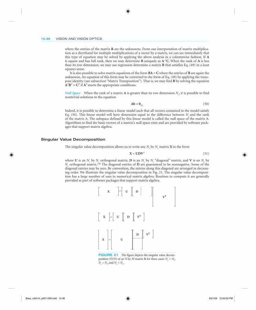
10.48 VISION AND VISION OPTICS
where the entries of the matrix B are the unknowns. From our interpretation of matrix multiplica-tion as a shorthand for multiple multiplications of a vector by a matrix, we can see immediately that this type of equation may be solved by applying the above analysis in a columnwise fashion. If A is square and has full rank, then we may determine B uniquely as A–1C. When the rank of A is less than its row dimension, we may use regression determine a matrix B that satisfies Eq. (49) in a least squares sense.
It is also possible to solve matrix equations of the form BA = C where the entries of B are again the unknowns. An equation of this form may be converted to the form of Eq. (49) by applying the trans-pose identity (see subsection “Matrix Transposition”). That is, we may find B by solving the equation ATBT = CT if AT meets the appropriate conditions.
Null Space When the rank of a matrix A is greater than its row dimension Nr, it is possible to find nontrivial solutions to the equation
Ab = 0Nr (50)
Indeed, it is possible to determine a linear model such that all vectors contained in the model satisfy Eq. (50). This linear model will have dimension equal to the difference between Nr and the rank of the matrix A. The subspace defined by this linear model is called the null space of the matrix A. Algorithms to find the basis vectors of a matrix’s null space exist and are provided by software pack-ages that support matrix algebra.
Singular Value Decomposition
The singular value decomposition allows us to write any Nr by Nc matrix X in the form
X = UDVT (51)
where U is an Nr by Nr orthogonal matrix, D is an Nr by Nc “diagonal” matrix, and V is an Nc by Nc orthogonal matrix.148 The diagonal entries of D are guaranteed to be nonnegative. Some of the diagonal entries may be zero. By convention, the entries along this diagonal are arranged in decreas-ing order. We illustrate the singular value decomposition in Fig. 21. The singular value decomposi-tion has a large number of uses in numerical matrix algebra. Routines to compute it are generally provided as part of software packages that support matrix algebra.
X = U D
X =
VT
X = U D VT
U
D VT
FIGURE 21 The figure depicts the singular value decom-position (SVD) of an N by M matrix X for three cases: Nc > Nr, Nc = Nr, and Nc < Nr.
Bass_v3ch10_p001-056.indd 10.48Bass_v3ch10_p001-056.indd 10.48 8/21/09 12:50:02 PM8/21/09 12:50:02 PM
COLORIMETRY 10.49
10.8 REFERENCES
1. J. von Kries, “Chromatic Adaptation,” 1902, reprinted in Sources of Color Vision, D. L. MacAdam, (ed.), MIT Press, 1970, Cambridge, MA, pp. 109–119.
2. R. M. Evans, An Introduction to Color, Wiley, New York, 1948.
3. G. Wyszecki, “Color Appearance,” in Handbook of Perception and Human Performance: Sensory Processes and Perception, K. R. Boff, L. Kaufman, and J. P. Thomas, (eds.), John Wiley & Sons, New York, 1986, pp. 9.1–9.56.
4. B. K. P. Horn, “Exact Reproduction of Colored Images,” Computer Vision, Graphics and Image Processing 26:135–167 (1984).
5. R. W. G. Hunt, The Reproduction of Colour, 4th ed., Fountain Press, Tolworth, England, 1987.
6. M. D. Fairchild, Color Appearance Models, Addison-Wesley, Reading, MA, 1998.
7. D. H. Brainard and B. A. Wandell, “Calibrated Processing of Image Color,” Color Research and Application 15:266–271 (1990).
8. G. Wyszecki and W. S. Stiles, Color Science—Concepts and Methods, Quantitative Data and Formulae, 2nd ed., John Wiley & Sons, New York, 1982.
9. V. C. Smith and J. Pokorny, “Color Matching and Color Discrimination,” in The Science of Color, 2nd ed., S. K. Shevell, (ed.), Optical Society of America; Elsevier Ltd, Oxford, 2003, pp. 103–148.
10. CIE, Colorimetry, 3rd edition, Publication 15.2004, Bureau Central de la CIE, Vienna, 2004.
11. CIE, Fundamental Chromaticity Diagram with Physiological Axes—Part 1, Publication 170–1, Bureau Central de la CIE, Vienna, 2006.
12. D. H. Krantz, “Color Measurement and Color Theory: I. Representation Theorem for Grassmann Structures,” Journal of Mathematical Psychology 12:283–303 (1975).
13. P. Suppes, D. H. Krantz, R. D. Luce, and A. Tversky, Foundations of Measurement, Academic Press, San Diego, 1989, Vol. II.
14. D. L. MacAdam, Sources of Color Science, MIT Press, Cambridge, MA, 1970.
15. W. D. Wright, “The Origins of the 1931 CIE System,” in Human Color Vision, 2nd ed., P. K. Kaiser and R. M. Boynton, (eds.), Optical Society of America, Washington, D.C., 1996, pp. 534–543.
16. J. D. Mollon, “The Origins of Modern Color Science,” in The Science of Color, 2nd ed., S. K. Shevell, (ed.), Optical Society of America; Elsevier Ltd, Oxford, 2003, pp. 1–39.
17. R. Hall, Illumination and Color in Computer Generated Imagery, Springer-Verlag, New York, 1989.
18. D. B. Judd and G. Wyszecki, Color in Business, Science, and Industry, John-Wiley and Sons, New York, 1975.
19. G. S. Brindley, Physiology of the Retina and the Visual Pathway, 2nd ed., Williams and Wilkins, Baltimore, 1970.
20. R. M. Boynton, “History and Current Status of a Physiologically Based System of Photometry and Colorimetry,” Journal of the Optical Society of America A 65:1609–1621 (1996).
21. A. Stockman and L. T. Sharpe, “Cone Spectral Sensitivities and Color Matching,” in Color Vision: From Genes To Perception, K. R. Gegenfurtner and L. T. Sharpe, (eds.), Cambridge University Press, Cambridge, MA, 1999, pp. 53–87.
22. B. A. Wandell, “The Synthesis and Analysis of Color Images,” IEEE Transactions on Pattern Analysis and Machine Intelligence 9:2–13 (1987).
23. S. Westland and C. Ripamonti, Computational Colour Science using MATLAB, John Wiley & Sons, 2004.
24. B. Noble and J. W. Daniel, Applied Linear Algebra, 2nd ed., Prentice-Hall, Inc., Englewood Cliffs, NJ, 1977.
25. G. H. Golub and C. F. van Loan, Matrix Computations, Johns Hopkins University Press, Baltimore, 1983.
26. W. K. Pratt, Digital Image Processing, John Wiley & Sons, New York, 1978.
27. W. H. Press, B. P. Flannery, S. A. Teukolsky, and W. T. Vetterling, Numerical Recipes in C: The Art of Scientific Computing, Cambridge University Press, Cambridge, MA, 1988.
28. G. Wyszecki and W. Stiles, Color Science—Concepts and Methods, Quantitative Data and Formulas, John Wiley & Sons, New York, 1967.
29. W. S. Stiles, “The Physical Interpretation of the Spectral Sensitivity Curve of the Eye,” in Transactions of the Optical Convention of the Worshipful Company of Spectacle Makers, Spectacle Maker’s Company, London, 1948, pp. 97–107.
Bass_v3ch10_p001-056.indd 10.49Bass_v3ch10_p001-056.indd 10.49 8/21/09 12:50:02 PM8/21/09 12:50:02 PM

10.50 VISION AND VISION OPTICS
30. D. E. Mitchell and W. A. H. Rushton, “Visual Pigments in Dichromats,” Vision Research 11:1033–1043 (1971).
31. W. D. Wright, “A Re-determination of the Trichromatic Coefficients of the Spectral Colours,” Transactions of the Optical Society 30:141–164 (1928–1929).
32. J. Guild, “The Colorimetric Properties of the Spectrum,” Philosophical Transactions of the Royal Society of London A 230:149–187 (1931).
33. W. S. Stiles, “Interim Report to the Commission Internationale de l’Éclairage Zurich, 1955, on the National Physical Laboratory’s Investigation of Colour-matching” (with an Appendix by W. S. Stiles & J. M. Burch) Optica Acta 2:168–181 (1955).
34. W. S. Stiles and J. M. Burch, “NPL Colour-matching Investigation: Final Report (1958),” Optica Acta 6:1–26 (1959).
35. J. C. Maxwell, “On the Theory of Compound Colours and the Relations of the Colours of the Spectrum,” Philosophical Transactions of the Royal Society of London 150:57–84 (1860).
36. J. G. Grassmann, “Theory of Compound Colors,” in MacAdam, D.L., (ed.), Sources of Color Vision, MIT Press: Cambridge, MA, 1970. (Originally published in Annalen der Physik und Chemie, 89:69–84 1853).
37. CIE, Commission Internationale de l’ Éclairage Proceedings, 1931, Cambridge University Press, Cambridge, MA, 1932.
38. D. B. Judd, “Report of U.S. Secretariat Committee on Colorimetry and Artificial Daylight,” Proceedings of the Twelfth Session of the CIE 1:11 (1951).
39. J. J. Vos, “Colorimetric and Photometric Properties of a 2° Fundamental Observer,” Color Research and Application 3:125–128 (1978).
40. ISO/CIE, CIE Standard Colorimetric Observers, Reference Number 10527, International Organization for Standardization, Geneva, 1991.
41. I. E. Abdou and W. K. Pratt, “Quantitative Design and Evaluation of Enhancement/Thresholding Edge Detectors,” Proceedings of the IEEE 67:753–763 (1979).
42. CIE, Commission Internationale de l’ Éclairage Proceedings, 1924, Cambridge University Press, Cambridge, MA, 1926.
43. H. G. Sperling, “An Experimental Investigation of the Relationship Between Colour Mixture and Luminous Efficiency,” in Visual Problems of Colour, vol. 1, Her Majesty’s Stationery Office, London, 1958, pp. 249–277.
44. A. Stockman, L. T. Sharpe, and C. C. Fach, “The Spectral Sensitivity of the Human Short-wavelength Cones,” Vision Research 39:2901–2927 (1999).
45. V. C. Smith, J. Pokorny, and Q. Zaidi, “How do Sets of Color-matching Functions Differ?,” in Colour Vision, J. D. Mollon and L. T. Sharpe, (eds.), Academic Press, London, 1983, pp. 93–105.
46. A. Stockman and L. T. Sharpe, “Spectral Sensitivities of the Middle- and Long-Wavelength Sensitive Cones Derived from Measurements in Observers of Known Genotype,” Vision Research 40:1711–1737 (2000).
47. P. DeMarco, J. Pokorny, and V. C. Smith, “Full-spectrum Cone Sensitivity Functions for X-chromosome-linked Anomalous Trichromats,” Journal of the Optical Society of America 9:1465–1476 (1992).
48. N. I. Speranskaya, “Determination of Spectrum Color Coordinates for Twenty-seven Normal Observers,” Optics and Spectroscopy 7:424–428 (1959).
49. O. N. Rood, Modern Chromatics, with Applications to Art and Industry, D. Appleton & Co., New York, 1879.
50. T. Young, “On the Theory of Light and Colours,” Philosophical Transactions of the Royal Society of London 92:12–48 (1802).
51. H. L. F. von Helmholtz, “On the Theory of Compound Colours,” Philosophical Magazine Series, 4 4:519–534 (1852).
52. J. C. Maxwell, “Experiments on Colours, as Perceived by the Eye, with Remarks on Colour-blindness,” Transactions of the Royal Society of Edinburgh 21:275–298 (1855).
53. V. Smith and J. Pokorny, “Spectral Sensitivity of the Foveal Cone Photopigments between 400 and 500 nm,” Vision Research 15:161–171 (1975).
54. J. C. Maxwell, “On the Theory of Colours in Relation to Colour-blindness. A letter to Dr. G. Wilson,” Transactions of the Royal Scottish Society of Arts 4:394–400 (1856).
55. J. Nathans, T. P. Piantanida, R. L. Eddy, T. B. Shows, and D. S. Hogness, “Molecular Genetics of Inherited Variation in Human Color Vision,” Science 232:203–210 (1986).
56. J. Nathans, D. Thomas, and D. S. Hogness, “Molecular Genetics of Human Color Vision: the Genes Encoding Blue, Green and Red Pigments,” Science 232:193–202 (1986).
Bass_v3ch10_p001-056.indd 10.50Bass_v3ch10_p001-056.indd 10.50 8/21/09 12:50:03 PM8/21/09 12:50:03 PM

COLORIMETRY 10.51
57. M. M. Bongard and M. S. Smirnov, “Determination of the Eye Spectral Sensitivity Curves from Spectral Mixture Curves,” Doklady Akademiia nauk S.S.S.R. 102:1111–1114 (1954).
58. A. Stockman, D. I. A. MacLeod, and N. E. Johnson, “Spectral Sensitivities of the Human Cones,” Journal of the Optical Society of America A 10:2491–2521 (1993).
59. A. König and C. Dieterici, “Die Grundempfindungen in Normalen und anomalen Farben Systemen und ihre Intensitats-Verthielung im Spectrum,” Z Psychol Physiol Sinnesorg 4:241–347 (1893).
60. P. J. Bouma, “Mathematical Relationship between the Colour Vision System of Trichromats and Dichromats,” Physica 9:773–784 (1942).
61. D. B. Judd, “Standard Response Functions for Protanopic and Deuteranopic Vision,” Journal of the Optical Society of America 35:199–221 (1945).
62. D. B. Judd, “Standard Response Functions for Protanopic and Deuteranopic Vision,” Journal of the Optical Society of America 39:505 (1949).
63. J. J. Vos and P. L. Walraven, “On the Derivation of the Foveal Receptor Primaries,” Vision Research 11:799–818 (1971).
64. O. Estévez, “On the Fundamental Database of Normal and Dichromatic Color Vision,” Ph.D., Amsterdam University, 1979.
65. J. J. Vos, O. Estevez, and P. L. Walraven, “Improved Color Fundamentals Offer a New View on Photometric Additivity,” Vision Research 30:937–943 (1990).
66. A. Stockman, D. I. A. MacLeod, and J. A. Vivien, “Isolation of the Middle- and Long-wavelength Sensitive Cones in Normal Trichromats,” Journal of the Optical Society of America A 10:2471–2490 (1993).
67. M. A. Webster and D. I. A. MacLeod, “Factors Underlying Individual Differences in the Color Matches of Normal Observers,” Journal of the Optical Society of America A 5:1722–1735 (1988).
68. G. Wald, “Human Vision and the Spectrum,” Science 101:653–658 (1945).
69. R. A. Bone and J. M. B. Sparrock, “Comparison of Macular Pigment Densities in the Human Eye,” Vision Research 11:1057–1064 (1971).
70. P. L. Pease, A. J. Adams, and E. Nuccio, “Optical Density of Human Macular Pigment,” Vision Research 27:705–710 (1987).
71. D. van Norren and J. J. Vos, “Spectral Transmission of the Human Ocular Media,” Vision Research 14:1237–1244 (1974).
72. B. H. Crawford, “The Scotopic Visibility Function,” Proceedings of the Physical Society of London B 62:321–334 (1949).
73. F. S. Said and R. A. Weale, “The Variation with Age of the Spectral Transmissivity of the Living Human Crystalline Lens,” Gerontologia 3:213–231 (1959).
74. J. Pokorny, V. C. Smith, and M. Lutze, “Aging of the Human Lens,” Applied Optics 26:1437–1440 (1987).
75. M. Alpern, “Lack of Uniformity in Colour Matching,” Journal of Physiology 288:85–105 (1979).
76. H. Terstiege, “Untersuchungen zum Persistenz- und Koeffizientensatz,” Die Farbe 16:1–120 (1967).
77. S. S. Miller, “Psychophysical Estimates of Visual Pigment Densities in Red-green Dichromats,” Journal of Physiology 223:89–107 (1972).
78. P. E. King-Smith, “The Optical Density of Erythrolabe Determined by a New Method,” Journal of Physiology 230:551–560 (1973).
79. P. E. King-Smith, “The Optical Density of Erythrolabe Determined by Retinal Densitometry Using the Self-screening Method,” Journal of Physiology 230:535–549 (1973).
80. V. Smith and J. Pokorny, “Psychophysical Estimates of Optical Density in Human Cones,” Vision Research 13:1099–1202 (1973).
81. S. A. Burns and A. E. Elsner, “Color Matching at High Luminances: Photopigment Optical Density and Pupil Entry,” Journal of the Optical Society of America A 10:221–230 (1993).
82. T. T. J. M. Berendschot, J. van der Kraats, and D. van Norren, “Foveal Cone Mosaic and Visual Pigment Density in Dichromats,” Journal of Physiology 492:307–314 (1996).
83. C. A. Curcio, K. R. Sloan, R. E. Kalina, and A. E. Hendrickson, “Human Photoreceptor Topography,” Journal of Comparative Neurology 292:497–523 (1990).
Bass_v3ch10_p001-056.indd 10.51Bass_v3ch10_p001-056.indd 10.51 8/21/09 12:50:03 PM8/21/09 12:50:03 PM

10.52 VISION AND VISION OPTICS
84. A. E. Elsner, S. A. Burns, and R. H. Webb, “Mapping Cone Photopigment Optical Density,” Journal of the Optical Society of America A 10:52–58 (1993).
85. M. Neitz, J. Neitz, and G. H. Jacobs, “Spectral Tuning of Pigments Underlying Red-green Color Vision,” Science 252:971–973 (1991).
86. S. C. Merbs and J. Nathans, “Absorption Spectra of Human Cone Photopigments,” Nature 356:433–435 (1992).
87. S. L. Merbs and J. Nathans, “Absorption Spectra of the Hybrid Pigments Responsible for Anomalous Color Vision,” Science 258:464–466 (1992).
88. J. Winderickx, D. T. Lindsey, E. Sanocki, D. Y. Teller, A. G. Motulsky, and S. S. Deeb, “Polymorphism in Red Photopigment Underlies Variation in Colour Matching,” Nature 356:431–433 (1992).
89. L. T. Sharpe, A. Stockman, H. Jägle, and J. Nathans, “Opsin Genes, Cone Photopigments, Color Vision, and Color Blindness,” in Color Vision: From Genes To Perception, K. R. Gegenfurtner and L. T. Sharpe, (eds.), Cambridge University Press, Cambridge, MA, 1999, pp. 3–51.
90. D. H. Brainard, A. Roorda, Y. Yamauchi, J. B. Calderone, A. Metha, M. Neitz, J. Neitz, D. R. Williams, and G. H. Jacobs, “Functional Consequences of the Relative Numbers of L and M Cones,” Journal of the Optical Society of America A 17:607–614 (2000).
91. M. Drummond-Borg, S. S. Deeb, and A. G. Motolsky, “Molecular Patterns of X Chromosome-linked Color Vision Genes among 134 Men of European Ancestry,” Proceedings of the National Academy of Sciences 86:983–987 (1989).
92. J. Neitz, M. Neitz, and G. H. Jacobs, “More than 3 Different Cone Pigments among People with Normal Color Vision,” Vision Research 33:117–122 (1993).
93. J. P. Macke and J. Nathans, “Individual Variation in the Size of the Human Red and Green Pigment Gene Array,” Investigative Ophthalmology and Visual Science 38:1040–1043 (1997).
94. A. B. Asenjo, J. Rim, and D. D. Oprian, “Molecular Determinants of Human Red/Green Color Discrimination,” Neuron 12:1131–1138 (1994).
95. L. T. Sharpe, A. Stockman, H. Jägle, H. Knau, and J. Nathans, “L, M, and L-M Hybrid Cone Photopigments in Man: Deriving lmax from Flicker Photometric Spectral Sensitivities,” Vision Research 39:3513–3525 (1999).
96. M. Neitz, J. Neitz, and G. H. Jacobs, “Genetic Basis of Photopigment Variations in Human Dichromats,” Vision Research 35:2095–2103 (1995).
97. A. Stockman, L. T. Sharpe, S. Merbs, and J. Nathans, “Spectral Sensitivities of Human Cone Visual Pigments Determined in vivo and in vitro,” in Vertebrate Phototransduction and the Visual Cycle, Part B. Methods in Enzymology, Vol. 316, K. Palczewski, (ed.), Academic Press, New York, 2000, pp. 626–650.
98. J. J. Kremers, T. Usui, H. P. Scholl, and L. T. Sharpe, “Cone Signal Contributions to Electrograms in Dichromats and Trichromats,” Investigative Ophthalmology and Visual Science 40:920–930 (1999).
99. A. Stockman, H. Jägle, M. Pirzer, and L. T. Sharpe, “The Dependence of Luminous Efficiency on Chromatic Adaptation,” Journal of Vision 8:1–26 (2008).
100. A. Reitner, L. T. Sharpe, and E. Zrenner, “Is Colour Vision Possible with Only Rods and Blue-sensitive Cones?,” Nature 352:798–800 (1991).
101. A. König, and C. Dieterici, “Die Grundempfindungen und ihre Intensitäts-Vertheilung im Spectrum,” Sitzungsberichte Akademie der Wissenschaften, Berlin 1886:805–829 (1886).
102. S. Ishihara, Tests for Colour-Blindness, Kanehara Shuppen Company, Ltd., Tokyo, 1977.
103. D. Farnsworth, “The Farnsworth-Munsell 100 Hue and Dichotomous Tests for Color Vision,” Journal of the Optical Society of America 33:568–578 (1943).
104. L. Rayleigh, “Experiments on Colour,” Nature 25:64–66 (1881).
105. J. B. Birch, Diagnosis of Defective Colour Vision, Oxford University Press, Oxford, 1993.
106. A. König, “Über den Menschlichen Sehpurpur und seine Bedeutung fur das Sehen,” Acadamie der Wissenschaften Sitzungsberichte 30:577–598 (1894).
107. E. N. Willmer, “Further Observations on the Properties of the Central Fovea in Colour-blind and Normal Subjects,” Journal of Physiology 110:422–446 (1950).
108. L. C. Thomson and W. D. Wright, “The Colour Sensitivity of the Retina within the Central Fovea of Man,” Journal of Physiology 105:316–331 (1947).
Bass_v3ch10_p001-056.indd 10.52Bass_v3ch10_p001-056.indd 10.52 8/21/09 12:50:03 PM8/21/09 12:50:03 PM

COLORIMETRY 10.53
109. D. Williams, D. I. A. MacLeod, and M. Hayhoe, “Foveal Tritanopia,” Vision Research 21:1341–1356 (1981).
110. D. I. Flitcroft, “The Interactions between Chromatic Aberration, Defocus and Stimulus Chromaticity: Implications for Visual Physiology and Colorimetry,” Vision Research 29:349–360 (1989).
111. D. R. Williams, N. Sekiguchi, W. Haake, D. H. Brainard, and O. Packer, “The Cost of Trichromacy for Spatial Vision,” in From Pigments to Perception, B. B. Lee and A. Valberg, (eds.), Plenum Press, New York, 1991, pp. 11–22.
112. D. H. Marimont and B. A. Wandell, “Matching Color Images—the Effects of Axial Chromatic Aberration,” Journal of the Optical Society of America A 11:3113–3122 (1994).
113. L. N. Thibos, M. Ye, X. X. Zhang, and A. Bradley, “The Chromatic Eye—a New Reduced-eye Model of Ocular Chromatic Aberation in Humans,” Applied Optics 31:3594–3667 (1992).
114. I. Powell, “Lenses for Correcting Chromatic Aberration of the Eye,” Applied Optics 20:4152–4155 (1981).
115. K. H. Ruddock, “The Effect of Age Upon Colour Vision. II. Changes with Age in Light Transmission of the Ocular Media,” Vision Research 5:47–58 (1965).
116. A. Knowles and H. J. A. Dartnall, “The Photobiology of Vision,” in The Eye, H. Davson, (ed.), Academic Press, New York, 1977, pp. 321–533.
117. H. J. A. Dartnall, “The Interpretation of Spectral Sensitivity Curves,” British Medical Bulletin 9:24–30 (1953).
118. R. J. W. Mansfield, “Primate Photopigments and Cone Mechanisms,” in The Visual System, A. Fein and J. S. Levine, (eds.), Alan R. Liss, New York, 1985.
119. E. F. MacNichol, Jr., “A Unifying Presentation of Photopigment Spectra,” Vision Research 26:1543–1556 (1986).
120. T. D. Lamb, “Photoreceptor Spectral Sensitivities: Common Shape in the Long-Wavelength Spectral Region,” Vision Research 35:3083–3091 (1995).
121. H. B. Barlow, “What Causes Trichromacy? A Theoretical Analysis using Comb-filtered Spectra,” Vision Research 22:635–643 (1982).
122. V. I. Govardovskii, N. Fyhrquist, T. Reuter, D. G. Kuzmin, and K. Donner, “In Search of the Visual Pigment Template,” Visual Neuroscience 17:509 –528 (2000).
123. J. Walraven, C. Enroth-Cugell, D. C. Hood, D. I. A. MacLeod, and J. L. Schnapf, “The Control of Visual Sensitivity. Receptoral and Postreceptoral Processes,” in Visual Perception: The Neurophysiological Foundations, L. Spillman and J. S. Werner, (eds.), Academic Press, San Diego, 1990, pp. 53–101.
124. A. M. Derrington, J. Krauskopf, and P. Lennie, “Colour-opponent Cells in the Dorsal Lateral Geniculate Nucleus of the Macque,” Journal of Physiology 329:22–23 (1982).
125. D. I. A. MacLeod and R. M. Boynton, “Chromaticity Diagram Showing Cone Excitation by Stimuli of Equal Luminance,” Journal of the Optical Society of America 69:1183–1186 (1979).
126. R. Luther, “Aus dem Gebiet der Farbreizmetrik,” Zeitschrift für Technische Physik 8:540–558 (1927).
127. J. Krauskopf, D. R. Williams, and D. W. Heeley, “Cardinal Directions of Color Space.,” Vision Research 22:1123–1131 (1982).
128. J. Krauskopf, D. R. Williams, M. B. Mandler, and A. M. Brown, “Higher Order Color Mechanisms,” Vision Research 26:23–32 (1986).
129. D. H. Brainard, “Cone Contrast and Opponent Modulation Color Spaces,” in Human Color Vision, 2nd ed., P. K. Kaiser and R. M. Boynton, Optical Society of America, Washington, D.C., 1996, pp. 563–579.
130. A. B. Poirson and B. A. Wandell, “The Ellipsoidal Representation of Spectral Sensitivity,” Vision Research 30:647–652 (1990).
131. R. Ramamoorthi and P. Hanrahan, “A Signal-processing Framework for Reflection,” ACM Transactions on Graphics 23:1004–1042 (2004).
132. R. O. Dror, A. S. Willsky, and E. H. Adelson, “Statistical Characterization of Real-world Illumination,” Journal of Vision 4:821–837 (2004).
133. R. W. Fleming, R. O. Dror, and E. H. Adelson, “Real-world Illumination and the Perception of Surface Reflectance Properties,” Journal of Vision 3:347–368 (2003).
134. R. W. Fleming, A. Torralba, and E. H. Adelson, “Specular Reflections and the Perception of Shape,” Journal of Vision 4:798–820 (2004).
Bass_v3ch10_p001-056.indd 10.53Bass_v3ch10_p001-056.indd 10.53 8/21/09 12:50:04 PM8/21/09 12:50:04 PM

10.54 VISION AND VISION OPTICS
135. B. Xiao and D. H. Brainard, “Surface Gloss and Color Perception of 3D Objects,” Visual Neuroscience 25:371–385 (2008).
136. I. Motoyoshi, S. Nishida, L. Sharan, and E. H. Adelson, “Image Statistics and the Perception of Surface Qualities,” Nature 447:206–209 (2007).
137. D. B. Judd, D. L. MacAdam, and G. W. Wyszecki, “Spectral Distribution of Typical Daylight as a Function of Correlated Color Temperature,” Journal of the Optical Society of America 54:1031–1040 (1964).
138. J. Cohen, “Dependency of the Spectral Reflectance Curves of the Munsell Color Chips,” Psychonomic Science 1:369–370 (1964).
139. K. L. Kelly, K. S. Gibson, and D. Nickerson, “Tristimulus Specification of the Munsell Book of Color from Spectrophotometric Measurements,” Journal of the Optical Society of America 33:355–376 (1943).
140. D. Nickerson, “Spectrophotometric Data for a Collection of Munsell Samples,” U.S. Department of Agriculture, 1957.
141. L. T. Maloney, “Evaluation of Linear Models of Surface Spectral Reflectance with Small Numbers of Parameters,” Journal of the Optical Society of America A 3:1673–1683 (1986).
142. E. L. Krinov, “Surface Reflectance Properties of Natural Formations,” National Research Council of Canada: Technical Translation TT–439 (1947).
143. J. P. S. Parkkinen, J. Hallikainen, and T. Jaaskelainen, “Characteristic Spectra of Munsell Colors,” Journal of the Optical Society of America 6:318–322 (1989).
144. T. Jaaskelainen, J. Parkkinen, and S. Toyooka, “A Vector-subspace Model for Color Representation,” Journal of the Optical Society of America A 7:725–730 (1990).
145. J. R. Magnus and H. Neudecker, Matrix Differential Calculus with Applications in Statistics and Econometrics, Wiley, Chichester, 1988.
146. T. W. Anderson, An Introduction to Multivariate Statistical Analysis, 2nd ed., John Wiley and Sons, New York, 1971.
147. R. A. Johnson and D. W. Wichern, Applied Multivariate Statistical Analysis, Prentice-Hall, Englewood Cliffs, NJ, 1988.
148. J. M. Chambers, Computational Methods for Data Analysis, John Wiley and Sons, New York, 1977.
149. D. H. Marimont and B. A. Wandell, “Linear Models of Surface and Illuminant Spectra,” Journal of the Optical Society of America A 9:1905–1913 (1992).
150. B. A. Wandell and D. H. Brainard, “Towards Cross-media Color Reproduction,” Presented at the OSA Applied Vision Topical Meeting, San Francisco, CA, 1989.
151. C. A. Parraga, G. Brelstaff, T. Troscianko, and I. R. Moorehead, “Color and Luminance Information in Natural Scenes,” Journal of the Optical Society of America A 15:563–569 (1998).
152. P. Longère and D. H. Brainard, “Simulation of Digital Camera Images from Hyperspectral Input,” in Vision Models and Applications to Image and Video Processing, C. J. van den Branden Lambrecht (ed.), Kluwer Academic, Boston, 2001, pp. 123–150.
153. D. H. Foster, S. M. C. Nascimento, and K. Amano, “Information Limits on Neural Identification of Colored Surfaces in Natural Scenes,” Visual Neuroscience 21:1–6 (2004).
154. D. Saunders and A. Hamber, “From Pigments to Pixels: Measurement and Display of the Colour Gamut of Paintings,” Proceedings of the SPIE: Perceiving, Measuring, and Using Color 1250:90–102 (1990).
155. R. Berns, “Rejuvenating Seurat’s Palette Using Color and Imaging Science: a Simulation,” in Seurat and the Making of La Grande Jatte, R. L. Herbert, (ed.), University of California Press, 2004, pp. 214–227.
156. D. H. Brainard, D. G. Pelli, and T. Robson, “Display Characterization,” in Encyclopedia of Imaging Science and Technology, J. Hornak, (ed.) Wiley, 2002, pp. 72–188.
157. ISO/CIE, CIE Standard Colorimetric Illuminants, Reference Number 10526, International Organization for Standardization, Geneva, 1991.
158. D. H. Brainard, B. A. Wandell, and W. B. Cowan, “Black Light: How Sensors Filter Spectral Variation of the Illuminant,” IEEE Transactions on Biomedical Engineering 36:140–149 (1989).
159. G. Wyszecki, “Evaluation of Metameric Colors,” Journal of the Optical Society of America 48:451–454 (1958).
160. S. A. Burns, J. B. Cohen, and E. N. Kuznetsov, “Multiple Metatmers: Preserving Color Matches Under Diverse Illuminants,” Color Research and Application 14:16–22 (1989).
Bass_v3ch10_p001-056.indd 10.54Bass_v3ch10_p001-056.indd 10.54 8/21/09 12:50:04 PM8/21/09 12:50:04 PM

COLORIMETRY 10.55
161. G. D. Finlayson and M. S. Drew, “The Maximum Ignorance Assumption with Positivity,” Presented at the 4th IS&T/SID Color Imaging Conference, Scottsdale, AZ, 1996, pp. 202–204.
162. J. A. S. Viggiano, “Minimal-knowledge Assumptions in Digital Still Camerage Characterization. I. Uniform Distribution, Toeplitz Correlation,” Presented at the 9th IS&T/SID Color Imaging Conference, Scottsdale, AZ, 2001, pp. 332–336.
163. X. Zhang and D. H. Brainard, “Bayesian Color-correction Method for Non-colorimetric Digital Image Sensors,” Presented at the 12th IS&T/SID Color Imaging Conference, Scottsdale, AZ, 2004, pp. 308–314.
164. M. H. Brill, “A Device Performing Illuminant-invariant Assessment of Chromatic Relations,” Journal of Theoretical Biology 71:473–478 (1978).
165. G. Buchsbaum, “A Spatial Processor Model for Object Colour Perception,” Journal of the Franklin Institute 310:1–26 (1980).
166. L. T. Maloney and B. A. Wandell, “Color Constancy: A Method for Recovering Surface Spectral Reflectances,” Journal of the Optical Society of America A 3:29–33 (1986).
167. H. C. Lee, “Method for Computing the Scene-illuminant Chromaticity from Specular Highlights,” Journal of the Optical Society of America A 3:1694–1699 (1986).
168. B. Funt and J. Ho, “Color from Black and White,” Presented at the International Conference on Computer Vision, Tampa, FL, 1988, pp. 2–8.
169. B. V. Funt and M. S. Drew, “Color Constancy Computation in Near-Mondrian Scenes Using a Finite Dimensional Linear Model,” Presented at the IEEE Conference on Computer Vision and Pattern Recognition, Ann Arbor, MI, 1988, pp. 544–549.
170. D. A. Forsyth, “A Novel Approach to Colour Constancy,” Presented at the International Conference on Computer Vision, Tampa, FL, 1988, pp. 9–18.
171. G. D. Finlayson, P. H. Hubel, and S. Hordley, “Color by correlation,” Presented at the IS&T/SID Fifth Color Imaging Conference, Scottsdale, AZ, 1997, pp. 6–11.
172. D. H. Brainard and W. T. Freeman, “Bayesian Color Constancy,” Journal of the Optical Society of America A 14:1393–1411 (1997).
173. M. Ebner, Color Constancy, Wiley, Chichester, UK, 2007.
174. M. D’Zmura and P. Lennie, “Mechanisms of Color Constancy,” Journal of the Optical Society of America A 3:1662–1672 (1986).
175. A. C. Hurlbert, “Computational Models of Color Constancy,” in Perceptual Constancy: Why Things Look As They Do, V. Walsh and J. Kulikowski, (eds.), Cambridge University Press, Cambridge, MA, 1998, pp. 283–322.
176. L. T. Maloney, “Physics-Based Approaches to Modeling Surface Color Perception,” in Color Vision: From Genes to Perception, K. T. Gegenfurtner and L. T. Sharpe, (eds.), Cambridge University Press, Cambridge, MA, 1999, pp. 387–416.
177. D. H. Brainard, J. M. Kraft, and P. Longère, “Color Constancy: Developing Empirical Tests of Computational Models,” in Colour Perception: Mind and the Physical World, R. Mausfeld and D. Heyer, (eds.), Oxford University Press, Oxford, 2003, pp. 307–334.
178. D. H. Brainard, P. Longere, P. B. Delahunt, W. T. Freeman, J. M. Kraft, and B. Xiao, “Bayesian Model of Human Color Constancy,” Journal of Vision 6:1267–1281 (2006).
179. D. L. MacAdam, “Visual Sensitivities to Color Differences in Daylight,” Journal of the Optical Society of America 32:247–274 (1942).
180. D. L. MacAdam, “Colour Discrimination and the Influence of Colour Contrast on Acuity” Documenta Ophthalmologica 3:214–233 (1949).
181. G. Wyszecki, “Matching Color Differences,” Journal of the Optical Society of America 55:1319–1324 (1965).
182. G. Wyszecki and G. H. Fielder, “New Color-matching Ellipses,” Journal of the Optical Society of America 61:1135–1152 (1971).
183. W. S. Stiles, “Color vision: The Approach Through Increment Threshold Sensitivity,” Proceedings National Academy of Sciences (USA) 45:100–114 (1959).
184. C. Noorlander and J. J. Koenderink, “Spatial and Temporal Discrimination Ellipsoids in Color Space,” Journal of the Optical Society of America 73:1533–1543 (1983).
185. A. B. Poirson, B. A. Wandell, D. Varner, and D. H. Brainard, “Surface Characterizations of Color Thresholds,” Journal of the Optical Society of America A 7:783–789 (1990).
Bass_v3ch10_p001-056.indd 10.55Bass_v3ch10_p001-056.indd 10.55 8/21/09 12:50:04 PM8/21/09 12:50:04 PM

10.56 VISION AND VISION OPTICS
186. A. R. Robertson, “The CIE 1976 Color-difference Formula,” Color Research and Application 2:7–11 (1977).
187. H. de Lange, “Research into the Dynamic Nature of the Human Fovea-cortex Systems with Intermittent and Modulated Light. I. Attenuation Characteristics with White and Coloured Light,” Journal of the Optical Society of America 48:777–784 (1958).
188. H. de Lange, “Research into the Dynamic Nature of the Human Fovea-cortex Systems with Intermittent and Modulated Light. II. Phase Shift in Brightness and Delay in Color Perception,” Journal of the Optical Society of America 48:784–789 (1958).
189. N. Sekiguchi, D. R. Williams, and D. H. Brainard, “Efficiency for Detecting Isoluminant and Isochromatic Interference Fringes,” Journal of the Optical Society of America A 10:2118–2133 (1993).
190. E. C. Carter and R. C. Carter, “Color and Conspicuousness,” Journal of the Optical Society of America 71:723–729 (1981).
191. A. B. Poirson and B. A. Wandell, “Task-Dependent Color Discrimination,” Journal of the Optical Society of America A 7:776–782 (1990).
192. A. L. Nagy and R. R. Sanchez, “Critical Color Differences Determined with a Visual Search Task,” Journal of the Optical Society of America A 7:1209–1217 (1990).
193. H. E. Smithson, S. S. Khan, L. T. Sharpe, and A. Sotckman, “Transitions between Color Categories Mapped with a Reverse Stroop Task,” Visual Neuroscience 23:453–460 (2006).
194. CIE, Improvement to Industrial Colour-Difference Evaluation, Publication 142, Bureau Central de la CIE, Vienna, 2001.
195. G. Wagner and R. M. Boynton, “Comparison of Four Methods of Heterochromatic Photometry,” Journal of the Optical Society of America 62:1508–1515 (1972).
196. W. Abney and E. R. Festing, “Colour Photometry,” Philosophical Transactions of the Royal Society of London 177:423–456 (1886).
197. W. Abney, Researches in Colour Vision, Longmans, Green, London, 1913, p. 418.
198. A. Dresler, “The Non-additivity of Heterochromatic Brightness,” Transactions of the Illuminating Engineering Society (London) 18:141–165 (1953).
199. R. M. Boynton and P. Kaiser, “Vision: The Additivity Law Made to Work for Heterochromatic Photometry with Bipartite Fields,” Science 161:366–368 (1968).
200. S. L. Guth, N. J. Donley, and R. T. Marrocco, “On Luminance Additivity and Related Topics,” Vision Research 9:537–575 (1969).
201. Y. Le Grand, “Spectral Luminosity,” in Visual Psychophysics, Handbook of Sensory Physiology, D. Jameson and L. H. Hurvich, (eds.), Springer-Verlag, Berlin, 1972, pp. 413–433.
202. J. Pokorny, V. C. Smith, and M. Lutze, “Heterochromatic Modulation Photometry,” Journal of the Optical Society of America A 6:1618–1623 (1989).
203. P. Lennie, J. Pokorny, and V. C. Smith, “Luminance,” Journal of the Optical Society of America A 10:1283–1293 (1993).
204. CIE, CIE 1988 2° Spectral Luminous Efficiency Function for Photopic Vision, Publication 86, Bureau Central de la CIE, Vienna, 1990.
205. J. Pokorny and V. C. Smith, “Colorimetry and Color Discrimination,” in Handbook of Perception and Human Performance, K. R. Boff, L. Kaufman, and J. P. Thomas, (eds.), John Wiley & Sons, 1986.
206. A. Stockman, “Colorimetry,” in The Optics Encyclopedia: Basic Foundations and Practical Applications, T. G. Brown, K. Creath, H. Kogelnik, M. A. Kriss, J. Schmit, and M. J. Weber, (eds.), Wiley-VCH, Berlin, 2003, pp. 207–226.
207. J. B. Cohen and W. E. Kappauf, “Metameric Color Stimuli, Fundamental Metamers, and Wyszecki’s Metameric Blacks: Theory, Algebra, Geometry, Application,” American Journal of Psychology 95:537–564 (1982).
Bass_v3ch10_p001-056.indd 10.56Bass_v3ch10_p001-056.indd 10.56 8/21/09 12:50:05 PM8/21/09 12:50:05 PM