David H. Bailey and Robert F. Lucas,...

David H. Bailey and Robert F. Lucas, Editors

Performance Tuning ofScientific Applications

List of Figures

4.1 GTC weak scaling, showing minimum and maximum times, onthe (a) Franklin XT4, (b) Intrepid BG/P, and (c) HyperionXeon systems. The total number of particles and grid pointsare increased proportionally to the number of cores, describinga fusion device the size of ITER at 32,768 cores. . . . . . . . 9

4.2 Olympus code architecture (left), vertebra input CT data(right) . . . . . . . . . . . . . . . . . . . . . . . . . . . . . . . 12

4.3 Olympus weak scaling, flop rates (left), run times (right), forthe Cray XT4 (Franklin), Xeon cluster (Hyperion) and IBMBG/P (Intrepid) . . . . . . . . . . . . . . . . . . . . . . . . . 15

4.4 Left: Gravitational radiation emitted during in binary blackhole merger, as indicated by the rescaled Weyl scalar r · Ψ4.This simulation was performed with the Cactus-Carpet infras-tructure with nine levels of AMR tracking the inspiralling blackholes. The black holes are too small to be visible in this fig-ure. [Image credit to Christian Reisswig at the Albert EinsteinInstitute.] Right: Volume rendering of the gravitational radia-tion during a binary black hole merger, represented by the realpart of Weyl scalar r · ψ4. [Image credit to Werner Benger atLouisiana State University.] . . . . . . . . . . . . . . . . . . . 18

4.5 Carpet benchmark with nine levels of mesh refinement show-ing(a) weak scaling performance on three examined platformsand (b) scalability relative to concurrency. For ideal scaling therun time should be independent of the number of processors.Carpet shows good scalability except on Hyperion. . . . . . . 19

4.6 CASTRO (a) Close-up of a single star in the CASTRO testproblem, shown here in red through black on the slice planesare color contours of density. An isosurface of the velocity mag-nitude is shown in brown, and the vectors represent the radially-inward-pointing self-gravity. (b) Number of grids for each CAS-TRO test problem. . . . . . . . . . . . . . . . . . . . . . . . . 21

4.7 CASTRO performance behavior with and without the gravitysolver using one (L1) and two (L2) levels of adaptivity on (a)Franklin and (b) Hyperion. (c) Shows scalability of the variousconfigurations. . . . . . . . . . . . . . . . . . . . . . . . . . . 24

i

ii

4.8 MILC performance and scalability using (a–b) small and (c–d)large problem configurations. . . . . . . . . . . . . . . . . . . 26

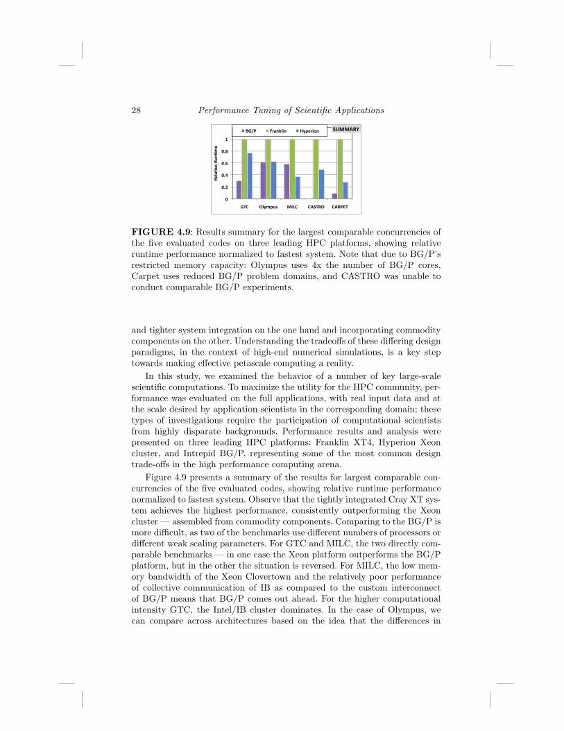
4.9 Results summary for the largest comparable concurrencies ofthe five evaluated codes on three leading HPC platforms, show-ing relative runtime performance normalized to fastest system.Note that due to BG/P’s restricted memory capacity: Olym-pus uses 4x the number of BG/P cores, Carpet uses reducedBG/P problem domains, and CASTRO was unable to conductcomparable BG/P experiments. . . . . . . . . . . . . . . . . . 28

List of Tables

4.1 Highlights of architectures and file systems for examined plat-forms. All bandwidths (BW) are in GB/s. “MPI BW” usesunidirection MPI benchmarks to exercise the fabric betweennodes with 0.5MB messages. . . . . . . . . . . . . . . . . . . . 5

4.2 Overview of scientific applications examined in our study . . 54.3 Scaled vertebral body mesh quantities. Number of cores used

on BG/P is four times greater than shown in this table. . . . 13

iii

Contents

4 Large-Scale Numerical Simulations on High-End Computa-tional Platforms 3Leonid Oliker, Jonathan Carter, Vincent Beckner, John Bell, Harvey

Wasseman, Mark Adams, Stephane Ethier, and Erik Schnetter4.1 Introduction . . . . . . . . . . . . . . . . . . . . . . . . . . . 34.2 HPC Platforms and Evaluated Applications . . . . . . . . . 44.3 GTC: Turbulent Transport in Magnetic Fusion . . . . . . . . 6

4.3.1 Gyrokinetic Toroidal Code . . . . . . . . . . . . . . . 64.4 GTC Performance . . . . . . . . . . . . . . . . . . . . . . . . 84.5 OLYMPUS: Unstructured FEM in Solid Mechanics . . . . . 11

4.5.1 Prometheus: parallel algebraic multigrid linear solver . 124.5.2 Olympus Performance . . . . . . . . . . . . . . . . . . 13

4.6 Carpet: Higher-Order AMR in Relativistic Astrophysics . . . 164.6.1 The Cactus Software Framework . . . . . . . . . . . . 164.6.2 Computational Infrastructure: Mesh Refinement with

Carpet . . . . . . . . . . . . . . . . . . . . . . . . . . . 164.6.3 Carpet Benchmark . . . . . . . . . . . . . . . . . . . . 174.6.4 Carpet Performance . . . . . . . . . . . . . . . . . . . 19

4.7 CASTRO: Compressible Astrophysics . . . . . . . . . . . . . 204.7.1 CASTRO and Carpet . . . . . . . . . . . . . . . . . . 224.7.2 CASTRO Performance . . . . . . . . . . . . . . . . . . 23

4.8 MILC: Quantum Chromodynamics . . . . . . . . . . . . . . 254.8.1 MILC Performance . . . . . . . . . . . . . . . . . . . . 26

4.9 Summary and Conclusions . . . . . . . . . . . . . . . . . . . 274.10 Acknowledgements . . . . . . . . . . . . . . . . . . . . . . . . 29

Bibliography 31

v

Chapter 4

Large-Scale Numerical Simulations onHigh-End Computational Platforms

Leonid Oliker, Jonathan Carter, Vincent Beckner, John Bell, Harvey Wasseman

CRD/NERSC, Lawrence Berkeley National Laboratory

Mark Adams

APAM Department, Columbia University

Stephane Ethier

Princeton Plasma Physics Laboratory, Princeton University

Erik Schnetter

CCT, Louisiana State University

4.1 Introduction . . . . . . . . . . . . . . . . . . . . . . . . . . . . . . . . . . . . . . . . . . . . . . . . . . . . . . . . . . . . . . . 34.2 HPC Platforms and Evaluated Applications . . . . . . . . . . . . . . . . . . . . . . . . . . . . . 44.3 GTC: Turbulent Transport in Magnetic Fusion . . . . . . . . . . . . . . . . . . . . . . . . . . 5

4.3.1 Gyrokinetic Toroidal Code . . . . . . . . . . . . . . . . . . . . . . . . . . . . . . . . . . . . . . . . 64.4 GTC Performance . . . . . . . . . . . . . . . . . . . . . . . . . . . . . . . . . . . . . . . . . . . . . . . . . . . . . . . . . 74.5 OLYMPUS: Unstructured FEM in Solid Mechanics . . . . . . . . . . . . . . . . . . . . . 11

4.5.1 Prometheus: parallel algebraic multigrid linear solver . . . . . . . . . . . . 124.5.2 Olympus Performance . . . . . . . . . . . . . . . . . . . . . . . . . . . . . . . . . . . . . . . . . . . . . 13

4.6 Carpet: Higher-Order AMR in Relativistic Astrophysics . . . . . . . . . . . . . . . . . 154.6.1 The Cactus Software Framework . . . . . . . . . . . . . . . . . . . . . . . . . . . . . . . . . 164.6.2 Computational Infrastructure: Mesh Refinement with Carpet . . . 164.6.3 Carpet Benchmark . . . . . . . . . . . . . . . . . . . . . . . . . . . . . . . . . . . . . . . . . . . . . . . . 174.6.4 Carpet Performance . . . . . . . . . . . . . . . . . . . . . . . . . . . . . . . . . . . . . . . . . . . . . . . 19

4.7 CASTRO: Compressible Astrophysics . . . . . . . . . . . . . . . . . . . . . . . . . . . . . . . . . . . . 204.7.1 CASTRO and Carpet . . . . . . . . . . . . . . . . . . . . . . . . . . . . . . . . . . . . . . . . . . . . . 224.7.2 CASTRO Performance . . . . . . . . . . . . . . . . . . . . . . . . . . . . . . . . . . . . . . . . . . . . 23

4.8 MILC: Quantum Chromodynamics . . . . . . . . . . . . . . . . . . . . . . . . . . . . . . . . . . . . . . . 254.8.1 MILC Performance . . . . . . . . . . . . . . . . . . . . . . . . . . . . . . . . . . . . . . . . . . . . . . . . 26

4.9 Summary and Conclusions . . . . . . . . . . . . . . . . . . . . . . . . . . . . . . . . . . . . . . . . . . . . . . . . 274.10 Acknowledgements . . . . . . . . . . . . . . . . . . . . . . . . . . . . . . . . . . . . . . . . . . . . . . . . . . . . . . . . 29

4.1 Introduction

After a decade where high-end computing was dominated by the rapidpace of improvements to CPU frequencies, the performance of next-generation

3

4 Performance Tuning of Scientific Applications

supercomputers is increasingly differentiated by varying interconnect designsand levels of integration. Understanding the tradeoffs of these system designsis a key step towards making effective petascale computing a reality. In thiswork, we conduct an extensive performance evaluation of five key scientificapplication areas: micro-turbulence fusion, quantum chromodynamics, micro-finite-element solid mechanics, supernovae and general relativistic astrophysicsthat use a variety of advanced computation methods, including adaptive meshrefinement, lattice topologies, particle in cell, and unstructured finite elements.Scalability results and analysis are presented on three current high-end HPCsystems, the IBM BlueGene/P at Argonne National Laboratory, the Cray XT4and the Berkeley Laboratory’s NERSC Center, and an Intel Xeon cluster atLawrence Livermore National Laboratory1. In this paper, we present each codeas a section, where we describe the application, the parallelization strategies,and the primary results on each of the three platforms. Then we follow witha collective analysis of the codes performance and make concluding remarks.

4.2 HPC Platforms and Evaluated Applications

In this section we outline the architecture of the systems used in thisstudy. We have chosen three three architectures which are often deployed athigh-performance computing installations, the Cray XT, IBM BG/P, and anIntel/Infiniband cluster. The cpu and node architectures are fully describedin Chapter ?? , Section ?? of this book, so we confine ourselves here to adescription of the interconnects. In selecting the systems to be benchmarked,we have attempted to cover a wide range of systems having different intercon-nects. The Cray XT is designed with tightly integrated node and interconnectfabric. Cray have opted to design a custom network ASIC and messagingprotocol and couple this with a commodity AMD processor. In contrast, theIntel/IB cluster is assembled from off the shelf high-perfortmance networkingcomponents and Intel server processors. The final system, BG/P, is customdesigned for processor, node and interconnect with power efficiency as one ofthe primary goals. Together these represent the most common design trade-offs in the high performance computing arena. Table 4.1 shows the size andtopology of the three system interconnects.

Franklin: Cray XT4: Franklin, a 9660 node Cray XT4 supercomputer,is located at Lawrence Berkeley National Laboratory (LBNL). Each XT4 nodecontains a quad-core 2.3 GHz AMD Opteron processor, which is tightly inte-grated to the XT4 interconnect via a Cray SeaStar2+ ASIC through a Hyper-Transport 2 interface capable of capable of 6.4 GB/s. All the SeaStar routing

1The Hyperion cluster used was configured with 45-nanometer Intel Xeon processor 5400series, which are quad-core “Harpertown nodes.”

Large-Scale Numerical Simulations on High-End Computational Platforms 5

System Processor Total MPIName Architecture

InterconnectNodes BW

Franklin Opteron Seastar2+/3D Torus 9660 1.67Intrepid BG/P 3D Torus/Fat Tree 40960 1.27Hyperion Xeon Infiniband 4×DDR 576 0.37

TABLE 4.1: Highlights of architectures and file systems for examinedplatforms. All bandwidths (BW) are in GB/s. “MPI BW” uses unidirectionMPI benchmarks to exercise the fabric between nodes with 0.5MB messages.

chips are interconnected in a 3D torus topology with each link is capable of7.6 GB/s peak bidirectional bandwidth, where each node has a direct linkto its six nearest neighbors. Typical MPI latencies will range from 4-8µs, de-pending on the size of the system and the job placement.

Intrepid: IBM BG/P: Intrepid is a BG/P system located at ArgonneNational Labs (ANL) with 40 racks of 1024 nodes each. Each BG/P node has 4PowerPC 450 CPUs (0.85 GHz) and 2GB of memory. BG/P implements threehigh-performance networks: a 3D torus with a peak bandwidth of 0.4 GB/sper link (6 links per node) for point to point messaging; a collectives networkfor broadcast and reductions with 0.85 GB/s per link (3 links per node); anda network for a low-latency global barrier. Typical MPI latencies will rangefrom 3-10µs, depending on the size of the system and the job placement.

Hyperion: Intel Xeon Cluster: The Hyperion cluster, located atLawrence Livermore National Laboratory (LLNL), is composed of four scal-able units, each consisting of 134 dual-socket nodes utilizing 2.5 GHz quad-core Intel Harpertown processors. The nodes within a scalable unit are fullyconnected via a 4× IB DDR network with an peak bidirectional bandwidth of2.0 GB/s. The scalable units are connected together via spine switches provid-ing full bisection bandwidth between scalable units. Typical MPI latencies willrange from 2-5µs, depending on the size of the system and the job placement.

The applications chosen as benchmarks come from diverse scientific do-mains and employ quite different numerical algorithms and are summarizedin Table 4.2.

Code ComputationalNameLines

DisciplineStructure

GTC 15,000 Magnetic Fusion Particle/GridOLYMPUS 30,000 Solid Mechanics Unstructured FECARPET 500,000 Relativistic Astrophysics AMR/GridCASTRO 300,000 Compressible Astrophysics AMR/Grid

MILC 60,000 Quantum Chromodynamics Lattice

TABLE 4.2: Overview of scientific applications examined in our study


4.3 GTC: Turbulent Transport in Magnetic Fusion

4.3.1 Gyrokinetic Toroidal Code

The Gyrokinetic Toroidal Code (GTC) is a 3D particle-in-cell (PIC) codedeveloped to study the turbulent transport properties of tokamak fusion de-vices from first principles [41, 42]. The current production version of GTCscales extremely well with the number of particles on the largest systemsavailable. It achieves this by using multiple levels of parallelism: a 1D domaindecomposition in the toroidal dimension (long way around the torus geom-etry), a multi-process particle distribution within each one of these toroidaldomains, and a loop-level multitasking implemented with OpenMP directives.The 1D domain decomposition and particle distribution are implemented withMPI using 2 different communicators: a toroidal communicator to move parti-cles from one domain to another, and an intra-domain communicator to gatherthe contribution of all the particles located in the same domain. Communica-tion involving all the processes is kept to a minimum. In the PIC method, agrid-based field is used to calculate the interaction between the charged par-ticles instead of evaluating the N2 direct binary Coulomb interactions. Thisfield is evaluated by solving the gyrokinetic Poisson equation [40] using theparticles’ charge density accumulated on the grid. The basic steps of the PICmethod are: (i) Accumulate the charge density on the grid from the contribu-tion of each particle to its nearest grid points. (ii) Solve the Poisson equationto evaluate the field. (iii) Gather the value of the field at the position of theparticles. (iv) Advance the particles by one time step using the equations ofmotion (“push” step). The most time-consuming steps are the charge accu-mulation and particle “push”, which account for about 80% to 85% of thetime as long as the number of particles per cell per process is about two orgreater.

In the original GTC version described above, the local grid within atoroidal domain is replicated on each MPI process within that domain and theparticles are randomly distributed to cover that whole domain. The grid work,which comprises of the field solve and field smoothing, is performed redun-dantly on each of these MPI processes in the domain. Only the particle-relatedwork is fully divided between the processes. This has not been an issue untilrecently due to the fact that the grid work is small when using a large numberof particles per cell. However, when simulating very large fusion devices, suchas the international experiment ITER [33], a much larger grid must be usedto fully resolve the microturbulence physics, and all the replicated copies ofthat grid on the processes within a toroidal domain make for a proportionallylarge memory footprint. With only a small amount of memory left on thesystem’s nodes, only a modest amount of particles per cell per process canfit. This problem is particularly severe on the IBM Blue Gene system wherethe amount of memory per core is small. Eventually, the grid work starts


dominating the calculation even if a very large number of processor cores isused.

The solution to our non-scalable grid work problem was to add anotherlevel of domain decomposition to the existing toroidal decomposition. Al-though one might think that a fully 3D domain decomposition is the idealchoice, the dynamics of magnetically confined charged particles in tokamakstells us otherwise. The particle motion is very fast in both the toroidal andpoloidal (short way around the torus) directions, but is fairly slow in the ra-dial direction. In the toroidal direction, the domains are large enough thatonly 10% of the particles on average leave their domain per time step in spiteof their high velocities. Poloidal domains would end up being much smaller,leading to a high level of communication due to a larger percentage of particlesmoving in and out of the domains at each step. Furthermore, the poloidal gridpoints are not aligned with each other in the radial direction, which makes thedelineation of the domains a difficult task. The radial grid, on the other hand,has the advantage of being regularly spaced and easy to split into several do-mains. The slow average velocity of the particles in that direction insures thatonly a small percentage of them will move in and out of the domains per timestep, which is what we observe.

One disadvantage, however, is that the radial width of the domains needsto decrease with the radius in order to keep a uniform number of particlesin each domain since the particles are uniformly distributed across the wholevolume. This essentially means that each domain will have the same volumebut a different number of grid points. For a small grid having a large numberof radial domains, it is possible that a domain will fall between two radialgrid points. Another disadvantage is that the domains require a fairly largenumber of ghost cells, from 3 to 8 on each side, depending on the maximumvelocity of the particles. This is due to the fact that our particles are not pointparticles but rather charged “rings”, where the radius of the ring correspondsto the Larmor radius of the particle in the magnetic field. We actually followthe guiding center of that ring as it moves about the plasma, and the radius ofthe ring changes according to the local value of the magnetic field. A particlewith a guiding center sitting close to the boundary of its radial domain canhave its ring extend several grid points outside of that boundary. We need totake that into account for the charge deposition step since we pick four pointson that ring and split the charge between them [40]. As for the field solve forthe grid quantities, it is now fully parallel and implemented with the Portable,Extensible Toolkit for Scientific Computation (PETSc) [50].

Overall, the implementation of the radial decomposition in GTC resultedin a dramatic increase in scalability for the grid work and decrease in thememory footprint of each MPI process. We are now capable of carrying outan ITER-size simulation of 130 million grid points and 13 billion particlesusing 32,768 cores on the BG/P system, with as little as 512 Mbytes percore. This would not have been possible with the old algorithm due to thereplication of the local poloidal grid (2 million points).


4.4 GTC Performance

Figure 4.1 shows a weak scaling study of the new version of GTC onFranklin, Intrepid, and Hyperion. In contrast with previous scaling studiesthat were carried out with the production version of GTC and where thecomputational grid was kept fixed [48, 49], the new radial domain decompo-sition in GTC allows us to perform a true weak scaling study where boththe grid resolution and the particle number are increased proportionally tothe number of processor cores. In this study, the 128-core benchmark uses0.52 million grid points and 52 million particles while the 131,072-core caseuses 525 million grid points and 52 billion particles. This spans three ordersof magnitude in computational problem size and a range of fusion toroidaldevices from a small laboratory experiment of 0.17 m in minor radius to anITER-size device of 2.7 m, and to even twice that number for the 131,072-core test parameters. A doubling of the minor radius of the torus increases itsvolume by 8 if the aspect ratio is kept fixed. The Franklin Cray XT4 numbersstop at the ITER-size case on 32,768 cores due to the number of processorsavailable on the system although the same number of cores can easily handlethe largest case since the amount of memory per core is much larger than onBG/P. The concurrency on Hyperion stops at 2048, again due to the limitednumber of cores on this system. It is worth mentioning that we did not usethe shared-memory OpenMP parallelism in this study although it is availablein GTC.

The results of the weak scaling study are presented as area plots of the wallclock times for the main steps in the time-advanced loop as the number of coresincreases from 128 to 32,768 in the case of the XT4, from 128 to 131,072 for theBG/P, and from 128 to 2048 for Hyperion. The main steps of the time loop are:accumulating the particles’ charge density on the grid (“charge” step, memoryscatter), solving the Poisson equation on the grid (“solve” step), smoothingthe potential (“smooth” step), evaluating the electric field on the grid (“field”step), advancing the particles by one time step (“push” phase including fieldgather), and finally, moving the particles between processes (“shift”). The firstthing we notice is that the XT4 is faster than the other 2 systems for the samenumber of cores. It is about 30% faster than Hyperion up to the maximum of2048 cores available on that system. Compared to BG/P, Franklin is 4 timesfaster at low core count but that gap decreases to 2.4 times faster at 32,768cores. This clearly indicates that the new version of GTC scales better onBG/P than Franklin, a conclusion that can be readily inferred visually fromthe area plots. The scaling on BG/P is impressive and shows the good balancebetween the processor speed and the network speed. Both the “charge” and“push” steps have excellent scaling on all three systems as can be seen fromthe nearly constant width of their respective areas on the plots although the“charge” step starts to increase at large processor count. The “shift” step


0

50

100

150

200

250

128 512 2K 8K 32K

Minim

um Run

/me (secon

ds)

Processors

GTC: Franklin MIN Other Smooth Solve

Field ShiH Charge

Push

0

50

100

150

200

250

128 512 2K 8K 32K

Maxim

um Run

1me (secon

ds)

Processors

GTC: Franklin MAX Other Smooth Solve

Field ShiI Charge

Push

(a)

0

100

200

300

400

500

600

700

128 512 2K 8K 32K 128K

Minim

um Run

2me (secon

ds)

Processors

GTC: BG/P MIN Other Smooth Solve Field ShiK Charge Push

0

100

200

300

400

500

600

700

128 512 2K 8K 32K 128K

Maxim

um Run

4me (secon

ds)

Processors

GTC: BG/P MAX Other Smooth Solve Field ShiM Charge Push

(b)

0

50

100

150

200

128 512 2K

Minim

um Run

.me (secon

ds)

Processors

GTC: Hyperion MIN Other Smooth Solve Field ShiH Charge Push

0

50

100

150

200

128 512 2K

Maxim

um Run

0me (secon

ds)

Processors

GTC: Hyperion MAX Other Smooth Solve Field ShiJ Charge Push

(c)

FIGURE 4.1: GTC weak scaling, showing minimum and maximum times,on the (a) Franklin XT4, (b) Intrepid BG/P, and (c) Hyperion Xeon systems.The total number of particles and grid points are increased proportionally tothe number of cores, describing a fusion device the size of ITER at 32,768cores.

also has very good scaling but the “smooth” and “field” steps account for the


largest degradation in the scaling at high processor counts. They also accountfor the largest differences between the minimum and maximum times spentby the MPI tasks in the main loop as can be seen by comparing the left(minimum times) and right (maximum times) plots for each system. Thesetwo steps hardly show up on the plots for the minimum times while they growsteadily on the plots for the maximum times. They make up for most of theunaccounted time on the minimum time plots, which shows up as “Other.”This indicates a growing load imbalance as the number of processor-coresincreases. We note that the “push” “charge” and “shift” steps involve almostexclusively particle-related work while “smooth” and “field” involve only grid-related work.

One might conclude that heavy communication is responsible for most ofthe load imbalance but we think otherwise due to the fact that grid workseems to be the most affected. We believe that the imbalance is due to alarge disparity in the number of grid points handled by the different processesat high core count. It is virtually impossible to have the same number ofparticles and grid points on each core due to the toroidal geometry of thecomputational volume and the radially decomposed domains. Since we requirea uniform density of grid points on the cross-sectional planes, this translatesto a constant arc length (and also radial length) separating adjacent gridpoints, resulting in less points on the radial surfaces near the center of thecircular plane compared to the ones near the outer boundary. Furthermore,the four-point average method used for the charge accumulation requires sixto eight radial ghost surfaces on each side of the radial zones to accommodateparticles with large Larmor radii. For large device sizes, this leads to largedifferences in the total number of grid points that the processes near the outerboundary have to handle compared to the processes near the center. Since theparticle work accounts for 80%–90% of the computational work, as shown bythe sum of the “push” “charge” and “shift” steps in the area plots, it is moreimportant to have the same number of particles in each radial domain ratherthan the same number of grid points. The domain decomposition in its currentimplementation thus targets a constant average number of particles during thesimulation rather than a constant number of grid points since both cannot beachieved simultaneously. It should be said, however, that this decompositionhas allowed GTC to simulate dramatically larger fusion devices on BG/P andthat the scaling still remains impressive.

The most communication intensive routine in GTC is the “shift” step,which moves the particles between the processes according to their new loca-tions after the time advance step. By looking at the plots of wall clock timesfor the three systems we immediately see that BG/P has the smallest ratio oftime spent in “shift” compared to the total loop time. This translates to thebest compute to communication ratio, which is to be expected since BG/Phas the slowest processor of the three systems. Hyperion, on the other hand,delivered the highest ratio of time spent in “shift”, indicating a network perfor-mance not as well balanced to its processor speed than the other two systems.


In terms of raw communication performance, the time spent in “shift” on theXT4 is about half of that on the BG/P at low core count. At high processorcount, the times are about the same. It is worth noting that on 131,072 coreson BG/P, process placement was used to optimize the communications whilethis was not yet attempted on Franklin at 32,768 cores.

4.5 OLYMPUS: Unstructured FEM in Solid Mechanics

Olympus is a finite element solid mechanics application that is used for,among other applications, micro-FE bone analysis [10, 18, 43]. Olympus is ageneral purpose, parallel, unstructured, finite element program and is used tosimulate bone mechanics via micro-FE methods. These methods generate fi-nite element meshes from micro-CT data that are composed of voxel elementsand accommodate the complex micro architecture of bone in much the sameway as pixels are used in a digital image. Olympus is composed of a paral-lelizing finite element module Athena. Athena uses a parallel graph partitioner(ParMetis [34]) to construct a sub-problem on each processor for a serial finiteelement code FEAP [30]. Olympus uses a parallel finite element object pFEAP,which is a thin parallelizing layer for FEAP, that primarily maps vector andmatrix quantities between the local FEAP grid and the global Olympus grid.Olympus uses the parallel algebraic multigrid linear solver Prometheus, whichis built on the parallel numerical library PETSc [17]. Olympus controls the so-lution process including an inexact Newton solver and manages the databaseoutput (SILO from LLNL) to be read by a visualization application (eg, VISITfrom LLNL). Figure 4.2 shows a schematic representation of this system.

The finite element input file is read, in parallel, by Athena which usesParMetis to partition the finite element graph. Athena generates a completefinite element problem on each processor from this partitioning. The processorsub-problems are designed so that each processor computes all rows of thestiffness matrix and entries of the residual vector associated with verticesthat have been partitioned to the processors. This eliminates the need forcommunication in the finite element operator evaluation at the expense ofa small amount of redundant computational work. Given this sub-problemand a small global text file with the material properties, FEAP runs on eachprocessor much as it would in serial mode; in fact FEAP itself has no parallelconstructs but only interfaces with Olympus through the pFEAP layer.

Explicit message passing (MPI) is used for performance and portabilityand all parts of the algorithm have been parallelized for scalability. Hierar-chical platforms, such as multi and many core architectures, are the intendedtarget for this project. Faster communication within a node is implicitly ex-ploited by first partitioning the problem onto the nodes, and then recursivelycalling Athena to construct the subdomain problem for each core. This ap-


(a) (b)

FIGURE 4.2: Olympus code architecture (left), vertebra input CT data(right)

proach implicitly takes advantage of any increase in communication perfor-mance within the node, though the numerical kernels (in PETSc) are pureMPI, and provides for good data locality.

4.5.1 Prometheus: parallel algebraic multigrid linear solver

The largest portion of the simulation time for these micro-FE bone prob-lems is spent in the unstructured algebraic multigrid linear solver Prometheus.Prometheus is equipped with three multigrid algorithms, has both additiveand (true) parallel multiplicative smoother preconditioners (general block andnodal block versions) [9], and several smoothers for the additive precondition-ers (Chebyshev polynomials are used in this study [11]).

Prometheus has been optimized for ultra-scalability, including two impor-tant features for complex problems using many processors [10]: (1) Prometheusrepartitions the coarse grids to maintain load balance and (2) the number ofactive processors, on the coarsest grids, is reduced to keep a minimum of afew hundred equations per processor. Reducing the number of active proces-sors on coarse grids is all but necessary for complex problems when usingtens or hundreds of thousands of cores, and is even useful on a few hundredcores. Repartitioning the coarse grids is important for highly heterogeneoustopologies because of severe load imbalances that can result from differentcoarsening rates in different domains of the problem. Repartitioning is alsoimportant on the coarsest grids when the number of processors are reduced


because, in general, the processor domains become fragmented which resultsin large amounts of communication in the solver.

4.5.2 Olympus Performance

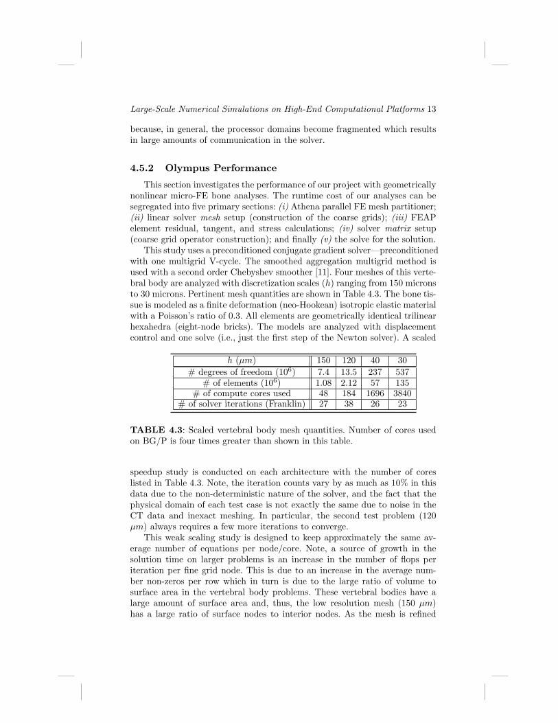
This section investigates the performance of our project with geometricallynonlinear micro-FE bone analyses. The runtime cost of our analyses can besegregated into five primary sections: (i) Athena parallel FE mesh partitioner;(ii) linear solver mesh setup (construction of the coarse grids); (iii) FEAPelement residual, tangent, and stress calculations; (iv) solver matrix setup(coarse grid operator construction); and finally (v) the solve for the solution.

This study uses a preconditioned conjugate gradient solver—preconditionedwith one multigrid V-cycle. The smoothed aggregation multigrid method isused with a second order Chebyshev smoother [11]. Four meshes of this verte-bral body are analyzed with discretization scales (h) ranging from 150 micronsto 30 microns. Pertinent mesh quantities are shown in Table 4.3. The bone tis-sue is modeled as a finite deformation (neo-Hookean) isotropic elastic materialwith a Poisson’s ratio of 0.3. All elements are geometrically identical trilinearhexahedra (eight-node bricks). The models are analyzed with displacementcontrol and one solve (i.e., just the first step of the Newton solver). A scaled

h (µm) 150 120 40 30# degrees of freedom (106) 7.4 13.5 237 537

# of elements (106) 1.08 2.12 57 135# of compute cores used 48 184 1696 3840

# of solver iterations (Franklin) 27 38 26 23

TABLE 4.3: Scaled vertebral body mesh quantities. Number of cores usedon BG/P is four times greater than shown in this table.

speedup study is conducted on each architecture with the number of coreslisted in Table 4.3. Note, the iteration counts vary by as much as 10% in thisdata due to the non-deterministic nature of the solver, and the fact that thephysical domain of each test case is not exactly the same due to noise in theCT data and inexact meshing. In particular, the second test problem (120µm) always requires a few more iterations to converge.

This weak scaling study is designed to keep approximately the same av-erage number of equations per node/core. Note, a source of growth in thesolution time on larger problems is an increase in the number of flops periteration per fine grid node. This is due to an increase in the average num-ber non-zeros per row which in turn is due to the large ratio of volume tosurface area in the vertebral body problems. These vertebral bodies have alarge amount of surface area and, thus, the low resolution mesh (150 µm)has a large ratio of surface nodes to interior nodes. As the mesh is refined


the ratio of interior nodes to surface nodes increases, resulting in, on aver-age, more non-zeros per row—from 50 on the smallest version to 68 on thelargest. Additionally, the complexity of the construction of the coarse grids insmoothed aggregation has the tendency to increase in fully 3D problems. Asthis problem is refined, the meshes become more fully 3D in nature—resultingin grids with more non-zeros per row and higher complexities—this would notbe noticeable with a fully 3D problem like a cube. Thus, the flop rates are abetter guide as to the scalability of the code and scalability of each machine.

Figure 4.3(a) shows the total flop rate of the solve phase and the matrixsetup phase (the two parts of the algorithm that are not amortized in a fullNewton nonlinear solve) on the Cray XT4 Franklin at NERSC. This showsvery good parallel efficiency from 48 to just under 4K cores and much higherflop rates for the matrix setup. The matrix setup uses small dense matrixmatrix multiplies (BLAS3) in its kernel which generally run faster than thedense matrix vector multiplies (BLAS2) in the kernel of the solve phase. Figure4.3(b) shows the times for the major components of a run with one linear solveron the Cray XT4. This data shows, as expected, good scalability (ie, constanttimes as problem size and processor counts are scaled up).

Figure 4.3(c) shows the flop rates for the solve phase and the matrix setupphase on the Xeon cluster Hyperion at LLNL. Again, we see much higher floprates for the matrix setup phase and the solve phase is scaling very well upto about 4K processors, but we do observe some degradation the performanceof the matrix setup on larger processor counts. This is due to the somewhatcomplex communication patterns required for the matrix setup as the finegrid matrix (source) and the course grid matrix (product) are partitionedseparately and load balancing becomes more challenging because the workper processor is not strictly proportional to the number of vertices on thatprocessor. Figure 4.3(d) shows the times for the major components of onelinear solver on Hyperion. This data shows that matrix setup phase is runningfast relative to the solve phase (relatively faster than on the Cray) and theAMG setup phase is slowing down on the larger processor counts. Overall theHyperion data shows that communication fabric is not as good as the Cray’sgiven that tasks with complex communication requirements are not scaling aswell on Hyperion as on the XT4.

Figure 4.3(e) shows the flop rates for the solve phase and the matrix setupphase on the IBM BG/P Intrepid at ANL. Figure 4.3(f) shows run times forthe solve phase and the matrix setup phase on the BG/P. Note, the scalingstudy on the BG/P uses four times as many cores as the other two tests, due tolack of memory. Additionally, we were not able to run the largest test case dueto lack of memory. These are preliminary results in that we have not addressedsome serious performance problems that we are observing on the IBM. Firstwe have observed fairly large load imbalance of about 30%. This imbalance ispartially due to the larger amount of parallelism demanded by the BG/P (i.e.,we have four times as many MPI processes as on the other systems). We doobserve good efficiency in the solve phase but we see significant growth in the


0.0

0.5

1.0

1.5

2.0

2.5

0 1000 2000 3000 4000 5000

MFlop

/sec

Processors

Olympus Franklin Scaling Matrix setup flops Matrix setup ideal Solve setup flop Solve setup ideal

(a)

0

10

20

30

40

50

60

48 184 1696 3840

Run.

me (secon

ds)

Processors

Olympus: Franklin Solve Matrix Setup AMG Setup

(b)

0.0

0.5

1.0

1.5

2.0

2.5

0 1000 2000 3000 4000 5000

MFlop

/sec

Processors

Olympus Hyperion Scaling Matrix setup flops

Matrix setup ideal

Solve setup flop

Solve setup ideal

(c)

0

10

20

30

40

50

60

48 184 1696 3840

Run.

me (secon

ds)

Processors

Olympus: Hyperion

Solve Matrix Setup AMG Setup

(d)

0.0

0.2

0.4

0.6

0.8

1.0

1.2

0 1000 2000 3000 4000 5000 6000 7000

MFlop

/sec

Processors

Olympus BG/P Scaling Matrix setup flops Matrix setup ideal Solve setup flop Solve setup ideal

(e)

0

10

20

30

40

50

60

192 660 6080

Run.

me (secon

ds)

Processors

Olympus: BG/P

Solve Matrix Setup

(f)

FIGURE 4.3: Olympus weak scaling, flop rates (left), run times (right), forthe Cray XT4 (Franklin), Xeon cluster (Hyperion) and IBM BG/P (Intrepid)

matrix setup phase. We speculate that this is due to load imbalance issues.Thus, we are seeing good scalability in the actual solve phase of the solverbut we are having problems with load balance and performance on the setupphases of the code. This will be the subject of future investigation.


4.6 Carpet: Higher-Order AMR in Relativistic Astro-physics

4.6.1 The Cactus Software Framework

Cactus [24, 31] is an open-source, modular, and portable programmingenvironment for collaborative HPC computing. It was designed and writ-ten specifically to enable scientists and engineers to develop and performthe large-scale simulations needed for modern scientific discovery across abroad range of disciplines. Cactus is used by a wide and growing rangeof applications, prominently including relativistic astrophysics, but also in-cluding quantum gravity, chemical engineering, lattice Boltzmann Methods,econometrics, computational fluid dynamics, and coastal and climate model-ing [16, 25, 29, 35, 36, 44, 51, 57]. The influence and success of Cactus in highperformance computing was recognized with the IEEE Sidney Fernbach prize,which was awarded to Edward Seidel at Supercomputing 2006.

Among the needs of the Cactus user community have been ease of use,portability, support of large and geographically diverse collaborations, andthe ability to handle enormous computing resources, visualization, file I/O,and data management. Cactus must also support the inclusion of legacy code,as well as a range of programming languages. Some of the key strengths ofCactus have been its portability and high performance, which led to it beingchosen by Intel to be one of the first scientific applications deployed on theIA64 platform, and Cactus’s widespread use for benchmarking computationalarchitectures. For example, a Cactus application was recently benchmarked onthe IBM BlueGene/P system at ANL and scaled well up to 131,072 processors.

Cactus is a so-called “tightly coupled” framework; Cactus applications aresingle executables that are intented to execute within one supercomputing sys-tem. Cactus components (called thorns) delegate their memory management,parallelism, and I/O to a specialized driver component. This architecture en-ables highly efficient component coupling with virtually no overhead.

The framework itself (called flesh) does not implement any significantfunctionality on its own. It rather offers a set of well-designed APIs whichare implemented by other components. The specific set of components whichare used to implement these can be decided at run time. For example, theseAPIs provide coordinate systems, generic interpolation, reduction operations,hyperslabbing, and various I/O methods, and more.

4.6.2 Computational Infrastructure: Mesh Refinement withCarpet

Carpet [6,55] is an adaptive mesh refinement (AMR) driver for the Cactusframework. Carpet is a driver for Cactus, providing adaptive mesh refinement,


memory management for grid functions, efficient parallelization, and I/O. Car-pet provides spatial discretization based on highly efficient block-structured,logically Cartesian grids. It employs a spatial domain decomposition usinga hybrid MPI/OpenMP parallelism. Time integration is performed via therecursive Berger–Oliger AMR scheme [21], including subcycling in time. Inaddition to mesh refinement, Carpet supports multi-patch systems [28,54,62]where the domain is covered by multiple, possibly overlapping, distorted, butlogically Cartesian grid blocks.

Cactus parallelizes its data structures on distributed memory architecturesvia spatial domain decomposition, with ghost zones added to each MPI pro-cess’ part of the grid hierarchy. Synchronization is performed automatically,based on declarations for each routine specifying variables it modifies, insteadof via explicit calls to communication routines.

Higher order methods require a substantial amount of ghost zones (inour case, three ghost zones for fourth order accurate, upwinding differencingstencils), leading to a significant memory overhead for each MPI process. Thiscan be counteracted by using OpenMP within a multi-core node, which isespecially attractive on modern systems with eight or more cores per node; allperformance critical parts of Cactus support OpenMP. However, non-uniformmemory access (NUMA) systems require care in laying out data structures inmemory to achieve good OpenMP performance, and we are therefore using acombination of MPI processes and OpenMP threads on such systems.

We have recently used Kranc [3, 32, 39] to generate a new Einstein solverMcLachlan [23,45]. Kranc is a Mathematica-based code generation system thatstarts from continuum equations in Mathematica notation, and automaticallygenerates full Cactus thorns after discretizing the equations. This approachshows a large potential, not only for reducing errors in complex systems ofequations, but also for reducing the time to implement new discretizationmethods such as higher-order finite differencing or curvilinear coordinate sys-tems. It furthermore enables automatic code optimizations at a very highlevel, using domain-specific knowledge about the system of equations and thediscretization method that is not available to the compiler, such as cache ormemory hierarchy optimizations or multi-core parallelization. Such optimiza-tions are planned for the future.

Section 4.7 below describes CASTRO, an AMR infrastructure using a sim-ilar algorithm. We also briefly compare both infrastructures there.

4.6.3 Carpet Benchmark

The Cactus–Carpet benchmark solves the Einstein equations, i.e., the fieldequations of General Relativity, which describe gravity near compact objectssuch as neutron stars or black holes. Far away from compact objects, the Ein-stein equations describe gravitational waves, which are expected to be detectedby ground-based and space-based detectors such as LIGO [4], GEO600 [2], and


FIGURE 4.4: Left: Gravitational radiation emitted during in binary blackhole merger, as indicated by the rescaled Weyl scalar r · Ψ4. This simulationwas performed with the Cactus-Carpet infrastructure with nine levels of AMRtracking the inspiralling black holes. The black holes are too small to be visiblein this figure. [Image credit to Christian Reisswig at the Albert Einstein Insti-tute.] Right: Volume rendering of the gravitational radiation during a binaryblack hole merger, represented by the real part of Weyl scalar r · ψ4. [Imagecredit to Werner Benger at Louisiana State University.]

LISA [5] in the coming years. This detection will have groundbreaking effectson our understanding, and open a new window onto the universe [59].

We use the BSSN formulation of the Einstein equations as described e.g. in[12,13], which is a set of 25 coupled second-order non-linear partial differentialequations. In this benchmark, these equations are discretized using higherorder finite differences on a block-structured mesh refinement grid hierarchy.Time integration uses Runge–Kutta type explicit methods. We further assumethat there is no matter or electromagnetic radiation present, and use radiative(absorbing) outer boundary conditions. We choose Minkowski (flat spacetime)initial conditions, which has no effect on the run time of the simulations.We use fourth order accurate spatial differencing, Berger–Oliger style meshrefinement [21] with subcycling in time, with higher order order Lagrangianinterpolation on the mesh refinement boundaries. We pre-define a fixed meshrefinement hierarchy with nine levels, each containing the same number ofgrid points. This is a weak scaling benchmark where the number of grid pointsincreases with the used number of cores. Figure 4.4 shows gravitational wavesfrom simulated binary black hole systems.

The salient features of this benchmark are thus: Explicit time inte-gration, finite differencing with mesh refinement, many variables (about 1GByte/core), complex calculations for each grid point (about 5000 flops). Thisbenchmark does not use any libraries in its kernel loop such as e.g. BLAS, LA-


0

50

100

150

200

250

300

64 256 1K 4K 8K

Run.

me (secon

ds)

Processors

CARPET

Franklin

BG/P

Hyperion

(a)

0

0.2

0.4

0.6

0.8

1

1.2

1.4

1.6

0 2000 4000 6000 8000

Scalab

ility

Processors

CARPET Scaling

Linear Franklin BG/P Hyperion

(b)

FIGURE 4.5: Carpet benchmark with nine levels of mesh refinement show-ing(a) weak scaling performance on three examined platforms and (b) scala-bility relative to concurrency. For ideal scaling the run time should be inde-pendent of the number of processors. Carpet shows good scalability except onHyperion.

PACK, or PETSc, since no efficient high-level libraries exist for stencil-basedcodes. However, we use automatic code generation [3, 32, 37, 39] which allowssome code optimizations and tuning at build time [15].

Our benchmark implementation uses the Cactus software framework[24, 31], the Carpet adaptive mesh refinement infrastructure [6, 54, 55], theEinstein Toolkit [1, 52], and the McLachlan Einstein code [45]. We describethis benchmark in detail in [58].

4.6.4 Carpet Performance

We examined the Carpet weak scaling benchmark described above on sev-eral systems with different architectures. Figure 4.5 shows results for the CrayXT4 Franklin, a Blue Gene/P, and Hyperion in terms of runtime and parallelscalability. Overall, Carpet shows excellent weak scalability, achieving super-linear performance on Franklin and Intrepid. On Hyperion scalability breaksdown at around 1024 processors, the source of the anomaly is under investiga-tion, as Carpet has demonstrated high scalability up to 12288 processors onother systems with similar architecture, including the Xeon/Infiniband QueenBee [7] and the AMD/Infiniband Ranger [8] clusters. We were unfortunatelynot able to obtain interactive access to Hyperion for the Cactus team, andwere thus not able to examine this problem in detail — future efforts willfocus on identifying the system-specific performance constraints.

We note that we needed to modify the benchmark parameters to run onthe BG/P system, since there is not enough memory per core for the standardsettings. Instead of assigning AMR components with 253 grid points to each


core, we were able to use only 133 grid points per component. This reducesthe per-core computational load by a factor of about eight, but reduces thememory consumption only by a factor of about four due to the additionalinter-processor ghost zones required. Consequently, we expect this smallerversion of the benchmark to show less performance and be less scalable.

In some cases (such as Franklin), scalability even improves for very largenumber of cores. We assume that it is due to the AMR interface conditionsin our problem setup. As the number of cores increases, we increase the totalproblem size to test weak scaling. Increasing the size of the domain by afactor of N increases the number of evolved grid points by N3, but increasesthe number of AMR interface points only by a factor of N2. As the problemsize increases, the importance of the AMR interface points (and the associatedcomputation and communication overhead) thus decreases.

4.7 CASTRO: Compressible Astrophysics

CASTRO is a finite volume evolution code for compressible flow in Euleriancoordinates and includes self-gravity and reaction networks. CASTRO incor-porates hierarchical block-structured adaptive mesh refinement and supports3D Cartesian, 2D Cartesian and cylindrical, and 1D Cartesian and sphericalcoordinates. It is currently used primarily in astrophysical applications, specif-ically for problems such as the time evolution of Type Ia and core collapsesupernovae.

The hydrodynamics in CASTRO is based on the unsplit methodology in-troduced in [26]. The code has options for the piecewise linear method in [26]and the unsplit piecewise parabolic method (PPM) in [46]. The unsplit PPMhas the option to use the less restrictive limiters introduced in [27]. All of thehydrodynamics options are designed to work with a general convex equationof state.

CASTRO supports two different methods for including Newtonian self-gravitational forces. One approach uses a monopole approximation to computea radial gravity consistent with the mass distribution. The second approachis based on solving the Poisson equation,

−∆φ = 4πGρ,

for the gravitational field, φ. The Poisson equation is discretized using stan-dard finite difference approximations and the resulting linear system is solvedusing geometric multigrid techniques, specifically V-cycles and red-blackGauss-Seidel relaxation. A third approach in which gravity is externally spec-ified is also available.

Our approach to adaptive refinement in CASTRO uses a nested hierarchy


(a)

Number Level1 Level2of Stars Grids Grids

512 (L0) 512 (L0)one 1728 (L1) 512 (L1)

1728 (L2)1024 1024

two 3456 10243456

2048 2048four 6912 2048

69124096 4096

eight 13824 409613824

(b)

FIGURE 4.6: CASTRO (a) Close-up of a single star in the CASTRO testproblem, shown here in red through black on the slice planes are color contoursof density. An isosurface of the velocity magnitude is shown in brown, and thevectors represent the radially-inward-pointing self-gravity. (b) Number of gridsfor each CASTRO test problem.

of logically-rectangular grids with simultaneous refinement of the grids in bothspace and time. The integration algorithm on the grid hierarchy is a recursiveprocedure in which coarse grids are advanced in time, fine grids are advancedmultiple steps to reach the same time as the coarse grids, and the data atdifferent levels are then synchronized. During the regridding step, increas-ingly finer grids are recursively embedded in coarse grids until the solutionis sufficiently resolved. An error estimation procedure based on user-specifiedcriteria evaluates where additional refinement is needed and grid generationprocedures dynamically create or remove rectangular fine grid patches as res-olution requirements change.

For pure hydrodynamic problems, synchronization between levels requiresonly a “reflux” operation in which coarse cells adjacent to the fine grid aremodified to reflect the difference between the original coarse-grid flux and theintegrated flux from the fine grid. (See [19, 20]). For processes that involveimplicit discretizations, the synchronization process is more complex. Thebasic synchronization paradigm for implicit processes is discussed in [14]. Inparticular, the synchronization step for the full self-gravity algorithm is similarto the algorithm introduced by [47].

CASTRO uses a general interface to equations of state and thermonuclear


reaction networks, that allows us to easily add more extensive networks tofollow detailed nucleosynthesis.

The parallelization strategy for CASTRO is to distribute grids to pro-cessors. This provides a natural coarse-grained approach to distributing thecomputational work. When AMR is used a dynamic load balancing techniqueis needed to adjust the load. We use both a heuristic knapsack algorithm anda space-filling curve algorithm for load balancing. Criteria based on the ratioof the number of grids at a level to the number of processors dynamicallyswitches between these strategies.

CASTRO is written in C++ and Fortran-90. The time stepping control,memory allocation, file I/O, and dynamic regridding operations occur primar-ily in C++. Operations on single arrays of data, as well as the entire multigridsolver framework, exist in Fortran-90.

4.7.1 CASTRO and Carpet

The AMR algorithms employed by CASTRO and Carpet (see section 4.6.1above) share certain features, and we outline the commonalities and differencesbelow.

Both CASTRO and Carpet use nested hierarchies of logically rectangulargrids, refining the grids in both space and time. The integration algorithmon the grid hierarchy is a recursive procedure in which coarse grids are firstadvanced in time, fine grids are then advanced multiple steps to reach the sametime as the coarse grids, and the data at different levels are then synchronized.This AMR methodology was introduced by Berger and Oliger (1984) [21] forhyperbolic problems.

Both CASTRO and Carpet support different coordinate systems; CAS-TRO can be used with Cartesian, cylindrical, or spherical coordinates whileCarpet can handle multiple patches with arbitrary coordinate systems [53].

The basic AMR algorithms in both CASTRO and Carpet is independentof the spatial discretization and the time integration methods which are em-ployed. This cleanly separates the formulation of physics from the computa-tional infrastructure which provides the mechanics of gridding and refinement.

The differences between CASTRO and Carpet are mostly historic in ori-gin, coming from the different applications areas that they are or were target-ing. CASTRO originates in the hydrodynamics community, whereas Carpet’sbackground is in solving the Einstein equations. This leads to differences inthe supported feature set, while the underlying AMR algorithm is very simi-lar. Quite likely both could be extended to support the feature set offered bythe respective other infrastructure.

For example, CASTRO offers a generic regridding algorithm based on user-specified criteria (e.g. to track shocks), refluxing to match fluxes on coarse andfine grids, vertex- and cell-centred quantities. These features are well suited tosolve flux-conservative hydrodynamics formulations. CASTRO also containsa full Poisson solver for Newtonian gravity.


Carpet, on the other hand, supports features required by the Einsteinequations, which have a wave-type nature where conservation is not relevant.Various formulations of the Einstein equations contain second spatial deriva-tives, requiring a special treatment of refinement boundaries (see [56]). Also,Carpet does not contain a Poisson solver since gravity is already described bythe Einstein equations, and no extra elliptic equation needs to be solved.

CASTRO and Carpet are also very similar in terms of their implementa-tion. Both are parallelised using MPI, and support for multi-core architecturesvia OpenMP has been or is being added.

4.7.2 CASTRO Performance

The test problem for the scaling study was that of one or more self-gravitating stars in a 3D domain with outflow boundary conditions on allsides. We used a stellar equation of state as implemented in [60] and initial-ized the simulation by interpolating data from a 1D model file onto the 3DCartesian mesh. The model file was generated by a 1D stellar evolution code,Kepler( [61]). An initial velocity perturbation was then superimposed ontothe otherwise quiescent star — a visualization is shown in Figure 4.6(a).

The test problem was constructed to create a weak scaling study, with asingle star in the smallest runs, and two, four, and eight stars for the largerruns, with the same grid layout duplicated for each star. Runs on Hyperionwere made with one, two, and four stars, using 400, 800, and 1600 processorsrespectively. Hyperion was in the early testing stage when these runs weremade and 1600 processors was the largest available pool at the time, so thesmaller runs were set to 400 and 800 processors. Runs on Franklin were madewith one, two, four, and eight stars, using 512, 1024, 2048, and 4096 processorsrespectively. The number of grids for each problem is shown in Table 4.6(b).

Figure 4.7 shows the performance and scaling behavior of CASTRO onFranklin and Hyperion. Results were not collected on Intrepid because thecurrent implementation of CASTRO is optimized for large grids and requiresmore memory per core than is available on that machine. This will be thesubject of future investigation. The runs labeled with “no gravity” do notinclude a gravity solver, and we note that these scale very well from 512to 4096 processors. Here Level1 refers to a simulation with a base level andone level of refinement, and Level2 refers to a base level and two levels ofrefinement. Refinement here is by a factor of two between each level. For theLevel2 calculations, the Level0 base grid size was set to half of the Level1calculation’s Level0 base size in each direction to maintian the same effectivecalculation resolution. Maximum grid size was 64 cells in each direction.

Observe that the runs with “gravity” use the Poisson solver and show lessideal scaling behavior; this is due to the increasing cost of communication inthe multigrid solver for solving the Poisson equation. However, the Level1 andLevel2 calculations show similar scaling, despite that fact that theLevel2 cal-culation has to do more communication than the Level1 calculation in order


0

50

100

150

200

250

300

350

512 1024 2048 4096

Run.

me (secon

ds)

Processors

CASTRO: Franklin

L1 No Gravity L1 Gravity L2 Gravity

(a)

0

50

100

150

200

250

300

350

400 800 1600

Run-

me (secon

ds)

Processors

CASTRO: Hyperion L1 No Gravity L1 Gravity L2 Gravity

(b)

0

0.2

0.4

0.6

0.8

1

1.2

0 1000 2000 3000 4000

Scalab

ility

Processors

CASTRO Scaling

Linear Franklin‐L2 Hyperion‐L2 Franklin‐L1‐NoGrav Hyperion‐L1‐NoGrav

(c)

FIGURE 4.7: CASTRO performance behavior with and without the gravitysolver using one (L1) and two (L2) levels of adaptivity on (a) Franklin and(b) Hyperion. (c) Shows scalability of the various configurations.

to syncronize the extra level and do more work to keep track of the overheaddata required by the extra level. The only exception to this is the highest con-currency Franklin benchmark, where the Level2 calculation scales noticeablyless well than the Level1.

Comparing the two architectures, Franklin shows the same or better scalingthan Hyperion for the one, two, and four star benchmarks despite using moreprocessors in each case. For the Level2 calculations with “gravity,” even at thelowest concurrency, Franklin is roughly 1.6 times faster than Hyperion, whilea performance prediction based on peak flops would be about 1.2.

In a real production calculation, the number and sizes of grids will varyduring the run as the underlying data evolves. This changes the calculation’soverall memory requirements, communication patterns, and sizes of commu-nicated data, and will therefore effect the overall performance of the entireapplication Future work will include investigations on optimal gridding, ef-fective utilization of shared memory multicore nodes, communication locality,


reduction of AMR metadata overhead requirements, and the introduction ofa hybrid MPI/OpenMP calculation model.

4.8 MILC: Quantum Chromodynamics

The MIMD Lattice Computation (MILC) collaboration has developed aset of codes written in the C language that are used to study quantum chromo-dynamics (QCD), the theory of the strong interactions of subatomic physics.“Strong interactions” are responsible for binding quarks into protons and neu-trons and holding them all together in the atomic nucleus. These codes aredesigned for use on MIMD (multiple instruction multiple data) parallel plat-forms, using the MPI library. A particular version of the MILC suite, enablingsimulations with conventional dynamical Kogut-Susskind quarks is studied inthis paper. The MILC code has been optimized to achieve high efficiency oncache-based superscalar processors. Both ANSI standard C and assembler-based codes for several architectures are provided in the source distribution.2

In QCD simulations, space and time are discretized on sites and linksof a regular hypercube lattice in four-dimensional space time. Each link be-tween nearest neighbors in this lattice is associated with a 3-dimensional SU(3)complex matrix for a given field [38]. The simulations involve integrating anequation of motion for hundreds or thousands of time steps that requires in-verting a large, sparse matrix at each step of the integration. The sparse matrixproblem is solved using a conjugate gradient (CG) method, but because thelinear system is nearly singular many CG iterations are required for conver-gence. Within a processor the four-dimensional nature of the problem requiresgathers from widely separated locations in memory. The matrix in the linearsystem being solved contains sets of complex 3-dimensional “link” matrices,one per 4-D lattice link but only links between odd sites and even sites arenon-zero. The inversion by CG requires repeated three-dimensional complexmatrix-vector multiplications, which reduces to a dot product of three pairsof three-dimensional complex vectors. The code separates the real and imag-inary parts, producing six dot product pairs of six-dimensional real vectors.Each such dot product consists of five multiply-add operations and one mul-tiply [22]. The primary parallel programing model for MILC is a 4-D domaindecomposition with each MPI process assigned an equal number of sublatticesof contiguous sites. In a four-dimensional problem each site has eight nearestneighbors.

Because the MILC benchmarks are intended to illustrate performanceachieved during the “steady-state” portion of an extremely long Lattice Gauge

2See http://www.physics.utah.edu/~detar/milc.html for a further description ofMILC.


0

1

2

3

4

5

6

7

128 512 2K 8K 32K

Run/

me (secon

ds)

Processors

MILC ‐ SMALL Hyperion

Franklin

BG/P

(a)

0

100

200

300

400

500

600

700

800

900

128 512 2K 8K 32K

Run0

me (secon

ds)

Processors

MILC ‐ LARGE Hyperion Franklin BG/P

(b)

0

0.2

0.4

0.6

0.8

1

1.2

0 2000 4000 6000 8000

Scalab

ility

Processors

MILC‐SMALL Scaling

Linear Hyperion Franklin BG/P

(c)

0

0.2

0.4

0.6

0.8

1

1.2

0 2000 4000 6000 8000

Scalab

ility

Processors

MILC‐LARGE Scaling

Linear Hyperion Franklin BG/P

(d)

FIGURE 4.8: MILC performance and scalability using (a–b) small and (c–d)large problem configurations.

simulation, each benchmark actually consists of two runs: a short run with afew steps, a large step size, and a loose convergence criterion to let the lat-tice evolve from a totally ordered state, and a longer run starting with this“primed” lattice, with increased accuracy for the CG solve and a CG iterationcount that is a more representative of real runs. Only the time for the latterportion is used.

4.8.1 MILC Performance

We conduct two weak-scaling experiments: a small lattice per core anda larger lattice per core, representing two extremes of how MILC might beused in a production configuration. Benchmark timing results and scalabilitycharacteristics are shown in Figures 4.8(a–b) and Figures 4.8(c–d) for smalland large problems, respectively. Not surprisingly, scalability is generally bet-ter for the larger lattice than for the smaller. This is particularly true for theFranklin XT4 system, for which scalability of the smaller problem is severely


limited. Although the overall computation/communication is very low, oneof the main sources of performance degradation is the CG solve. MILC wasinstrumented to measure the time in five major parts of the code, and on 1024cores the CG portion is consuming about two-thirds of the runtime. Micro-kernel benchmarking of the MPI Allreduce operation on three systems (notshown) shows that the XT4’s SeaStar interconnect is considerably slower onthis operation at larger core counts. Note, however, that these microkerneldata were obtained on a largely dedicated Hyperion system and a dedicatedpartition of BG/P but in a multi-user environment on the XT4, for which jobscheduling is basically random within the interconnect’s torus; therefore, theXT4 data likely include the effects of interconnect contention. For the smallerMILC lattice scalability suffers due to the insufficient computation, requiredto hide this increased Allreduce cost on the XT4.

In contrast, scalability doesn’t differ very much between the two latticesizes on the BG/P system, and indeed, scalability of the BG/P system isgenerally best of all the systems considered here. Furthermore, it is known thatcarefully mapping the 4-D MILC decomposition to the BG/P torus networkcan sometimes improve performance; however, this was not done in thesestudies and will be the subject of future investigations.

The Hyperion cluster shows similar scaling characteristics to Franklin forthe large case, and somewhat better scaling than Franklin for the small.

Turning our attention to absolute performance, for the large case we seethat Franklin significantly outperforms the other platforms, with the BG/Psystem providing the second best performance. For the small case, the or-der is essentially reversed, with Hyperion having the best performance acrossthe concurrencies studied. MILC is a memory bandwidth-intensive applica-tion. Nominally, the component vector and corresponding matrix operationsconsume 1.45 bytes input/flop and 0.36 bytes output/flop; in practice, wemeasure for the entire code a computational intensity of about 1.3 and 1.5,respectively, for the two lattice sizes on the Cray XT4. On multicore sys-tems this memory bandwidth dependence leads to significant contention ef-fects within the socket. The large case shows this effect most strongly, withthe Intel Harpertown-based Hyperion system lagging behind the other twoarchitectures despite having a higher peak floating-point performance.

4.9 Summary and Conclusions

Computational science is at the dawn of petascale computing capability,with the potential to achieve simulation scale and numerical fidelity at hithertounattainable levels. However, increasing concerns over power efficiency and theeconomies of designing and building these large systems are accelerating recenttrends towards architectural diversity through new interest in customization


0

0.2

0.4

0.6

0.8

1

GTC Olympus MILC CASTRO CARPET

Rela=ve Run

=me

SUMMARY BG/P Franklin Hyperion

FIGURE 4.9: Results summary for the largest comparable concurrencies ofthe five evaluated codes on three leading HPC platforms, showing relativeruntime performance normalized to fastest system. Note that due to BG/P’srestricted memory capacity: Olympus uses 4x the number of BG/P cores,Carpet uses reduced BG/P problem domains, and CASTRO was unable toconduct comparable BG/P experiments.

and tighter system integration on the one hand and incorporating commoditycomponents on the other. Understanding the tradeoffs of these differing designparadigms, in the context of high-end numerical simulations, is a key steptowards making effective petascale computing a reality.

In this study, we examined the behavior of a number of key large-scalescientific computations. To maximize the utility for the HPC community, per-formance was evaluated on the full applications, with real input data and atthe scale desired by application scientists in the corresponding domain; thesetypes of investigations require the participation of computational scientistsfrom highly disparate backgrounds. Performance results and analysis werepresented on three leading HPC platforms: Franklin XT4, Hyperion Xeoncluster, and Intrepid BG/P, representing some of the most common designtrade-offs in the high performance computing arena.

Figure 4.9 presents a summary of the results for largest comparable con-currencies of the five evaluated codes, showing relative runtime performancenormalized to fastest system. Observe that the tightly integrated Cray XT sys-tem achieves the highest performance, consistently outperforming the Xeoncluster — assembled from commodity components. Comparing to the BG/P ismore difficult, as two of the benchmarks use different numbers of processors ordifferent weak scaling parameters. For GTC and MILC, the two directly com-parable benchmarks — in one case the Xeon platform outperforms the BG/Pplatform, but in the other the situation is reversed. For MILC, the low mem-ory bandwidth of the Xeon Clovertown and the relatively poor performanceof collective communication of IB as compared to the custom interconnectof BG/P means that BG/P comes out ahead. For the higher computationalintensity GTC, the Intel/IB cluster dominates. In the case of Olympus, wecan compare across architectures based on the idea that the differences in


number of processors used is representative of how a simulation would be runin practice. Here BG/P and the Xeon cluster have comparable performance,with the XT ahead. For Carpet, the smaller domain sizes used for the BG/Pruns makes accurate comparison impossible, but one can certainly say thatabsolute performance is very poor compared with both the XT and Xeoncluster.

However, as the comparison in Figure 4.9 is at relatively small concurren-cies due to the size of the Intel/IB cluster, this is only part of the picture.At higher concurrencies the scalability of BG/P exceeds that of the XT forGTC and MILC, and substantially similar scaling is seen for Olympus. How-ever, for Carpet, XT scalability is better than on BG/P, although it should benoted that both scale superlinearly. While both BG/P and XT have custominterconnects, BG/P isolates portions of the interconnect (called partitions)for particular jobs much more effectively than on the XT, where nodes ina job can be scattered across the torus intermixed with other jobs that arecompeting for link bandwidth. This is one of the likely reasons for the poorerscalability of some applications on the XT.

Overall, these extensive performance evaluations are an important steptoward effectively conducting simulations at the petascale level and beyond,by providing computational scientists and system designers with critical in-formation on how well numerical methods perform across state-of-the-art par-allel systems. Future work will explore a wider set of computational methods,with a focus on irregular and unstructured algorithms, while investigating abroader set of HEC platforms, including the latest generation of multi-coretechnologies.

4.10 Acknowledgements

We thank Bob Walkup and Jun Doi of IBM for the optimized versionof MILC for the BG/P system and Steven Gottlieb of Indiana University formany helpful discussions related to MILC benchmarking. We also kindly thankBrent Gorda of LLNL for access to the Hyperion system. This work was sup-ported by the Advanced Scientific Computing Research Office in the DOE Of-fice of Science under contract number DE-AC02-05CH11231. The GTC workwas supportred by the DOE Office of Fusions Energy Science under contractnumber DE-AC02-09CH11466. This work was also supported by the NSFawards 0701566 XiRel and 0721915 Alpaca, by the LONI numrel allocation,and by the NSF TeraGrid allocations TG-MCA02N014 and TG-ASC090007.This research used resources of NERSC at LBNL and ALCF at ANL whichare supported by the Office of Science of the DOE under Contract No. DE-AC02-05CH11231 and DE-AC02-06CH11357 respectively.

Bibliography

[1] CactusEinstein toolkit home page. URL http://www.cactuscode.org/Community/

NumericalRelativity/.

[2] GEO 600. URL http://www.geo600.uni-hannover.de/.

[3] Kranc: Automated code generation. URL http://numrel.aei.mpg.de/Research/

Kranc/.

[4] LIGO: Laser Interferometer Gravitational wave Observatory. URL http://www.ligo.

caltech.edu/.

[5] LISA: Laser Interferometer Space Antenna. URL http://lisa.nasa.gov/.

[6] Mesh refinement with Carpet. URL http://www.carpetcode.org/.

[7] Queen Bee, the core supercomputer of LONI. URL http://www.loni.org/systems/

system.php?system=QueenBee.

[8] Sun Constellation Linux Cluster: Ranger. URL http://www.tacc.utexas.edu/

resources/hpc/.

[9] M. F. Adams. A distributed memory unstructured Gauss–Seidel algorithm for multi-grid smoothers. In ACM/IEEE Proceedings of SC2001: High Performance Networkingand Computing, Denver, Colorado, November 2001.

[10] M. F. Adams, H.H. Bayraktar, T.M. Keaveny, and P. Papadopoulos. Ultrascalableimplicit finite element analyses in solid mechanics with over a half a billion degrees offreedom. In ACM/IEEE Proceedings of SC2004: High Performance Networking andComputing, 2004.

[11] M. F. Adams, M. Brezina, J.J Hu, and R. S. Tuminaro. Parallel multigrid smoothing:polynomial versus Gauss–Seidel. J. Comp. Phys., 188(2):593–610, 2003.

[12] Miguel Alcubierre, Bernd Brugmann, Peter Diener, Michael Koppitz, Denis Pollney,Edward Seidel, and Ryoji Takahashi. Gauge conditions for long-term numerical blackhole evolutions without excision. Phys. Rev. D, 67:084023, 2003.

[13] Miguel Alcubierre, Bernd Brugmann, Thomas Dramlitsch, Jose A. Font, PhilipposPapadopoulos, Edward Seidel, Nikolaos Stergioulas, and Ryoji Takahashi. Towards astable numerical evolution of strongly gravitating systems in general relativity: Theconformal treatments. Phys. Rev. D, 62:044034, 2000.

[14] A. S. Almgren, J. B. Bell, P. Colella, L. H. Howell, and M. Welcome. A conserva-tive adaptive projection method for the variable density incompressible Navier-Stokesequations. Journal of Computational Physics, 142:1–46, 1998.

[15] Alpaca: Cactus tools for application-level profiling and correctness analysis. URLhttp://www.cct.lsu.edu/~eschnett/Alpaca/.

[16] Astrophysics Simulation Collaboratory (ASC) home page. URL http://www.

ascportal.org.

[17] Satish Balay, Kris Buschelman, Victor Eijkhout, William D. Gropp, Dinesh Kaushik,Matthew G. Knepley, Lois Curfman McInnes, Barry F. Smith, and Hong Zhang. PETScusers manual. Technical Report ANL-95/11 - Revision 3.0.0, Argonne National Labo-ratory, 2008.

31


[18] H. H. Bayraktar, M.F. Adams, P.F. Hoffmann, D.C. Lee, A. Gupta, P. Papadopoulos,and T.M. Keaveny. Micromechanics of the human vertebral body. In Transactions ofthe Orthopaedic Research Society, volume 29, page 1129, San Francisco, 2004.

[19] J. Bell, M. Berger, J. Saltzman, and M. Welcome. A three-dimensional adaptive meshrefinement for hyperbolic conservation laws. SIAM J. Sci. Statist. Comput., 15(1):127–138, 1994.

[20] M. J. Berger and P. Colella. Local adaptive mesh refinement for shock hydrodynamics.Journal of Computational Physics, 82(1):64–84, May 1989.

[21] Marsha J. Berger and Joseph Oliger. Adaptive mesh refinement for hyperbolic partialdifferential equations. J. Comput. Phys., 53:484–512, 1984.

[22] C. Bernard, C. DeTar, S. Gottlieb, U.M. Heller, J. Hetrick, N. Ishizuka, L. Karkkainen,S.R. Lantz, K. Rummukainen, R. Sugar, D. Toussaint, and M. Wingate. Lattice QCDon the IBM scalable POWERParallel systems SP2. In ACM/IEEE Proceedings of SC1995: High Performance Networking and Computing, San Diego, California, November1995.

[23] David Brown, Peter Diener, Olivier Sarbach, Erik Schnetter, and Manuel Tiglio. Tur-duckening black holes: an analytical and computational study. Phys. Rev. D (submit-ted), 2008. URL http://arxiv.org/abs/0809.3533.

[24] Cactus Computational Toolkit home page, URL http://www.cactuscode.org/.

[25] Karen Camarda, Yuan He, and Kenneth A. Bishop. A parallel chemical reactor simu-lation using Cactus. In Proceedings of Linux Clusters: The HPC Revolution, NCSA,2001. URL http://www.cactuscode.org/Articles/Camarda01.doc.

[26] P. Colella. Multidimensional Upwind Methods for Hyperbolic Conservation Laws.Journal of Computational Physics, 87:171–200, 1990.

[27] P. Colella and M. D. Sekora. A limiter for PPM that preserves accuracy at smoothextrema. Journal of Computational Physics, submitted.

[28] Peter Diener, Ernst Nils Dorband, Erik Schnetter, and Manuel Tiglio. Optimizedhigh-order derivative and dissipation operators satisfying summation by parts, andapplications in three-dimensional multi-block evolutions. J. Sci. Comput., 32:109–145,2007.

[29] Fokke Dijkstra and Aad van der Steen. Integration of Two Ocean Models. In SpecialIssue of Concurrency and Computation, Practice & Experience, volume 18, pages 193–202. Wiley, 2005.

[30] FEAP. URL http://www.ce.berkeley.edu/projects/feap/.

[31] T. Goodale, G. Allen, G. Lanfermann, J. Masso, T. Radke, E. Seidel, and J. Shalf. TheCactus framework and toolkit: Design and applications. In Vector and Parallel Pro-cessing – VECPAR’2002, 5th International Conference, Lecture Notes in ComputerScience, Berlin, 2003. Springer.

[32] Sascha Husa, Ian Hinder, and Christiane Lechner. Kranc: a Mathematica applicationto generate numerical codes for tensorial evolution equations. Comput. Phys. Comm.,174:983–1004, 2006.

[33] ITER: International thermonuclear experimental reactor. URL http://www.iter.org/.

[34] G. Karypis and V. Kumar. Parallel multilevel k-way partitioning scheme for irregu-lar graphs. ACM/IEEE Proceedings of SC1996: High Performance Networking andComputing, 1996.

[35] Jong G. Kim and Hyoung W. Park. Advanced simulation technique for modelingmultiphase fluid flow in porous media. In Computational Science and Its Applications- Iccsa 2004, LNCS 2004, by A. Lagana et. al., pages 1–9, 2004.


[36] Soon-Heum Ko, Kum Won Cho, Young Duk Song, Young Gyun Kim, Jeong su Na,and Chongam Kim. Lecture Notes in Computer Science: Advances in Grid Computing- EGC 2005: European Grid Conference, Amsterdam, The Netherlands, February 14-16, 2005, Revised Selected Papers, chapter Development of Cactus Driver for CFDAnalyses in the Grid Computing Environment, pages 771–777. Springer, 2005.

[37] Kranc: Automated code generation. URL http://www.cct.lsu.edu/~eschnett/

Kranc/.

[38] A.S. Kronfeld. Quantum chromodynamics with advanced computing. J. Phys.: Conf.Ser., 125:012067, 2008.

[39] Christiane Lechner, Dana Alic, and Sascha Husa. From tensor equations to numericalcode — computer algebra tools for numerical relativity. In SYNASC 2004 — 6th Inter-national Symposium on Symbolic and Numeric Algorithms for Scientific Computing,Timisoara, Romania, 2004. URL http://arxiv.org/abs/cs.SC/0411063.

[40] W. W. Lee. Gyrokinetic particle simulation model. J. Comp. Phys., 72:243–269, 1987.

[41] Z. Lin, S. Ethier, T.S. Hahm, and W.M. Tang. Size scaling of turbulent transport inmagnetically confined plasmas. Phys. Rev. Lett., 88, 2002.

[42] Z. Lin, T. S. Hahm, W. W. Lee, et al. Turbulent transport reduction by zonal flows:Massively parallel simulations. Science, 281:1835–1837, 1998.

[43] X.S. Liu, X.H. Zhang, K.K. Sekhon, M.F. Adam, D.J. McMahon, E. Shane, J.P.Bilezikian, and X.E. Guo. High-resolution peripheral quantitative computed tomogra-phy can assess microstructural and mechanical properties of human distal tibial bone.Journal of Bone and Mineral Research, in press.

[44] Seth Major, David Rideout, and Sumati Surya. Spatial hypersurfaces in causal setcosmology. Classical Quantum Gravity, 23:4743–4752, Jun 2006.

[45] McLachlan, a public BSSN code. URL http://www.cct.lsu.edu/~eschnett/

McLachlan/.

[46] G. H. Miller and P. Colella. A Conservative Three-Dimensional Eulerian Method forCoupled Solid-Fluid Shock Capturing. Journal of Computational Physics, 183:26–82,2002.

[47] F. Miniati and P. Colella. Block structured adaptive mesh and time refinement forhybrid, hyperbolic + n-body systems. Journal of Computational Physics, 227:400–430, 2007.

[48] L. Oliker, A. Canning, J. Carter, et al. Scientific Application Performance on CandidatePetaScale Platforms. In IPDPS:International Conference on Parallel and DistributedComputing Systems, Long Beach, CA, 2007.

[49] L. Oliker, A. Canning, J. Carter, and J. Shalf. Scientific computations on modernparallel vector systems. In Proc. SC2004, Pittsburgh, PA, 2004.

[50] PETSc: Portable, extensible toolkit for scientific computation. URL http://www.mcs.

anl.gov/petsc/.

[51] D. Rideout and S. Zohren. Evidence for an entropy bound from fundamentally discretegravity. Classical Quantum Gravity, 2006.

[52] Erik Schnetter. Multi-physics coupling of Einstein and hydrodynamics evolution: Acase study of the Einstein Toolkit. CBHPC 2008 (Component-Based High PerformanceComputing) (accepted), 2008.

[53] Erik Schnetter, Peter Diener, Ernst Nils Dorband, and Manuel Tiglio. A multi-blockinfrastructure for three-dimensional time-dependent numerical relativity. ClassicalQuantum Gravity, 23:S553–S578, 2006. URL http://arxiv.org/abs/gr-qc/0602104.

[54] Erik Schnetter, Peter Diener, Nils Dorband, and Manuel Tiglio. A multi-block infras-tructure for three-dimensional time-dependent numerical relativity. Classical QuantumGravity, 23:S553–S578, 2006. URL http://stacks.iop.org/CQG/23/S553.


[55] Erik Schnetter, Scott H. Hawley, and Ian Hawke. Evolutions in 3D numerical relativityusing fixed mesh refinement. Classical Quantum Gravity, 21(6):1465–1488, 21 March2004.

[56] Erik Schnetter, Scott H. Hawley, and Ian Hawke. Evolutions in 3d numerical relativityusing fixed mesh refinement. Classical Quantum Gravity, 21:1465–1488, 2004. URLhttp://arxiv.org/abs/gr-qc/0310042.

[57] B. Talbot, S. Zhou, and G. Higgins. Review of the Cactus framework: Software en-gineering support of the third round of scientific grand challenge investigations, task4 report - earth system modeling framework survey. URL http://ntrs.nasa.gov/

archive/nasa/casi.ntrs.nasa.gov/20020069014_2002111115.pdf.

[58] Jian Tao, Gabrielle Allen, Ian Hinder, Erik Schnetter, and Yosef Zlochower. XiRel:Standard benchmarks for numerical relativity codes using Cactus and Carpet. Techni-cal Report CCT-TR-2008-5, Louisiana State University, 2008. URL http://www.cct.

lsu.edu/CCT-TR/CCT-TR-2008-5.

[59] K. S. Thorne. Gravitational Radiation – a New Window Onto the Universe. (KarlSchwarzschild Lecture 1996). Reviews of Modern Astronomy, 10:1–28, 1997.

[60] Frank X. Timmes and F. Douglas Swesty. The accuracy, consistency, and speed of anelectron-positron equation of state based on table interpolation of the helmholtz freeenergy. ”Astrophysical Journal, Supplement”, 126:501–516, 2000.

[61] T. A. Weaver, G. B. Zimmerman, and S. E. Woosley. Presupernova evolution of massivestars. Astrophysical Journal, 225:1021–1029, 1978.

[62] Burkhard Zink, Erik Schnetter, and Manuel Tiglio. Multipatch methods in generalrelativistic astrophysics – hydrodynamical flows on fixed backgrounds. Phys. Rev. D,77:103015, 2008.

David H. Bailey and Robert F. Lucas,...

Documents

Transcript of David H. Bailey and Robert F. Lucas,...