Dating chicks: Calibration and discrimination in a nonlinear multivariate hierarchical growth model

Dating Chicks: Calibration andDiscrimination in a Nonlinear Multivariate

Hierarchical Growth Model

Geoffrey JONES, Rachel J. KEEDWELL,Alasdair D. L. NOBLE, and Duncan I. HEDDERLEY

The motivation for this work was to investigate the possibility of accurately deter-mining the age of a tern chick using easily obtained body measurements. We describe theconstruction of a nonlinear multivariate hierarchical model for chick growth and show howit can be estimated using Markov chain Monte Carlo techniques. A simple extension of theanalysis allows for estimation of the ages of unknown chicks. Posterior distributions of theunknown ages are derived, so that the accuracy of age determination can be examined. Wefurther extend our model and analysis to include the possibility that chicks fall into distinctgroups with different growth characteristics. The technique is illustrated using data on theweight and wing length of black-fronted terns from the Ohau River, New Zealand. It isfound that dating to within one day is possible, but only in some areas of the data space. Theconcept of “braiding” of multivariate growth curves is introduced to explain the varyingaccuracy of age determination.

Key Words: Inverse regression; Longitudinal; Mixed effects; Multilevel; Multiresponsemodel; Markov chain Monte Carlo; Repeated measures.

1. INTRODUCTION

The black-fronted tern (Sterna albostriata) is an endangered bird species whose habitatis the braided river systems of New Zealand’s South Island. Keedwell (2002) studied thegrowth and survival rates of tern chicks, knowledge of which are important in assessingfuture management techniques for increasing chick survival. This article focuses on thevariability in growth rates and the accuracy with which chick age can be determined usingeasily obtained body measurements. A nonlinear multiresponse model is used to describe

Geoffrey Jones is Senior Lecturer, Institute of Information Sciences and Technology, Massey University, PrivateBag 11222, Palmerston North, NZ (E-mail: [email protected]). Rachel J. Keedwell is an Ecological Con-sultant, P.O. Box 5539, Palmerston North, NZ (E-mail: [email protected]). Alasdair D. L. Noble isLecturer, Institute of Information Sciences and Technology, Massey University, Private Bag 11222, PalmerstonNorth, NZ (E-mail: [email protected]). Duncan I. Hedderley is Biometrician, NZ Institute of Crop andFood Research Ltd., Private Bag 11600, Palmerston North, NZ (E-mail: [email protected]).

©2005 American Statistical Association and the International Biometric SocietyJournal of Agricultural, Biological, and Environmental Statistics, Volume 10, Number 3, Pages 306–320DOI: 10.1198/108571105X59035

306

DATING CHICKS 307

the weight and wing length of tern chicks as functions of age. Inverse regression estimatesfrom this model can then be used to date chicks based on their weight and wing length.

Growth-curve modeling is an application of nonlinear regression in which a morpho-logical measurement is assumed to be a nonlinear, usually parametric, function of age.Typically the chosen function has an unknown upper asymptote, so is nonlinear in its pa-rameters. Some of the commonly used functions, such as the Gompertz, logistic and vonBertalanffy can be motivated as the solution of a differential equation describing the rate ofgrowth. The general theory of nonlinear regression, including growth curve modeling, wasgiven by Seber and Wild (1989).

If the available data comprise a series of measurements on each of a number of individ-uals, the model needs to allow different parameters for each individual to reflect populationheterogeneity. Suchmodels are variously known asmixed effects, repeatedmeasures, longi-tudinal, or hierarchical models, and have beenwidely studied (Laird andWare 1982; Diggle,Liang, and Zeger 1994; Goldstein 1995; Davidian and Giltinan 1995). Applications to non-linear growth curves in a biological context were given by Lindstrom and Bates (1990), whoillustrated their numerical algorithm for maximizing an approximate marginal likelihoodwith an analysis of the trunk circumference growth of orange trees, and Palmer, Phillips,and Smith (1991) who fit hierarchical models to growth data on emus, noisy scrub-birds,and whelks using the EM algorithm. Computational issues in the estimation of nonlinearmixed effects models were discussed by Pinheiro and Bates (1995). Software for fitting suchmodels to univariate longitudinal data is now widely available (Wolfinger 1999; Pinheiroand Bates 2000). Recently Markov chain Monte Carlo (MCMC) techniques have becomepopular for fitting hierarchicalmodels. Examples in the fitting of linear and nonlinear growthcurves are given in the BUGS program (Spiegelhalter, Thomas, Best, and Gilks 1994).

The simultaneous growth-curve modeling of multiple body measurements does notseem to have been widely considered. Wood (1982) investigated only the linear, nonhier-archical case. Clarke (1992) fitted nonlinear population growth curves to the lengths of thehorns of two-horned rhinos, but again not hierarchical. The data here can be regarded assamples from response curves traced out in the data space by varying the age parameter, asituation similar to that investigated by Ladd and Lindstrom (2000) for speech kinematicsdata using self-modeling regression. Davidian and Giltinan (1995, pp. 261–272) gave anexample of a bivariate hierarchical nonlinear pharmacokinetics model which is very sim-ilar to our situation. Extensive research has been done in statistical genetics on modelingrepeated measures of a single trait in order to investigate the time-dependence of geneticvariance components, and this could be extended to multiple traits, but in these models therandom components are additive and linear in parameters. A thorough review was given byJaffrézic and Pletcher (2000).

Determination of the age of further individuals from an estimated growth model is anapplication of statistical calibration or inverse regression, the theory of which was summa-rized by Brown (1993). Wood (1982) and Clarke (1992) investigated age determination inthe linear and nonlinear cases, respectively. Palmer et. al (1991) also considered the possibil-ity of multiple possible recaptures, with initial age as unobserved data in their EM approach.

308 G. JONES, R. J. KEEDWELL, A. D. L. NOBLE, AND D. I. HEDDERLEY

Menzefricke (1999) demonstrated the use of MCMC methods for inverse regression in aunivariate linear (in parameters) hierarchical model, using as an example the tensile indexof paper pulp as a function of beating time.

In some instances the population might comprise distinct groups with different growthcharacteristics, that is, with the random growth parameters drawn from different under-lying distributions. For example, males and females might exhibit quite different rates ofgrowth. In many cases, such as gender, group membership may be clearly determinablefrom distinguishing phenotypic characteristics, but in other cases, such as birth order, itmay be necessary to estimate not only the age but also the group membership of unknownindividuals. A similar situation, but with fixed curve parameters, was addressed by Jonesand Rocke (2001) for identifying and quantitating herbicides usingmultiple immunoassays.

In this article, we use MCMC to fit a bivariate nonlinear hierarchical model to theweight and wing length of tern chicks, allowing for the possibility of two distinct popu-lations, and use the model to investigate the achievable accuracy of age determination forthis population. Section 2 presents the general modeling and estimation framework, withthe application to tern chick growth illustrated in Section 3. Section 4 discusses inverseregression estimation and the discrimination problem. Finally, the results and methodologyare discussed in Section 5.

2. A MULTIVARIATE HIERARCHICAL GROWTH MODEL

Suppose we have repeated measurements {(yij , tij), t = 1, . . . , ni} on individualsi = 1, . . . , I , where yij is a p-dimensional vector comprising the measurements of p bodyparts made on individual i at time tij . We assume

yij = f(tij ;θi,ψ) + εij , (2.1)

whereθi is a vector of individual-specific growth parameters,ψ a vector of fixed parameters,f(.) a vector-valued function with p components, and ε a p-dimensional random error.We further assume that the individual-specific parameters are randomly drawn from somepopulation, specifically a multivariate normal distribution with mean θ0 and covariance ΣΣΣ,and that the errors are independent and normally distributed with mean zero and covarianceV.

In most cases components of θi and ψ will affect only one component of f(.). Thesefunctional forms would be chosen either from initial univariate analyses or from the litera-ture, and the parameters they contain would usually have meanings specific to a particularbody part. There may be exceptions. Clarke (1992) achieved parsimony by assuming a com-mon asymptote for the lengths of the horns of two-horned rhinos. In any case we can expecthigh correlations between some of the random growth parameters for different componentsof f(.), since fast growers will tend to be fast in every dimension. This can be a problem infitting these models because it can lead to near-singularity inΣΣΣ. Another difficulty is the po-tentially large number of parameters involved. We shall see in Section 3 that careful choiceof the functional forms and their parameterization can reduce these problems substantially.

DATING CHICKS 309

Figure 1. Graphical model for a multivariate hierarchical growth model with two measurements Y1,ij , Y2,ij

made on each chick at times xij . Here, for ease of exposition, it is assumed that Y1,ij , Y2,ij are conditionallyindependent given the growth parameters.

A related, but different, issue is the correlation between the estimates of parameters for asingle individual, which again can be reduced by reparameterization. To take the simplestcase of linear growth, the correlation between estimates for a single line could be reducedby mean-centering age, that is, by replacing αi + βitij by αi + βi(tij − t̄), so that α ismeasuring size at age t̄. However, it may be that in the population initial size is uncorre-lated with rate of growth, so that mean-centering actually increases the correlation in ΣΣΣ. Byreducing correlation between the estimates mean-centering can speed up convergence, butwe chose to retain initial size as it is a biologically meaningful parameter which we thoughtmight be uncorrelated with growth rate.

In applying MCMC methodology for the estimation of the model parameters ψ, θ0,ΣΣΣ, V we adopt a Bayesian framework, specifying prior distributions p(ψ), p(θ0), p(ΣΣΣ),p(V) on these parameters. We have used diffuse normal priors (σ = 103) for the growthparameters p(ψ), p(θ0) and inverse-Wishart priors with small degrees of freedom (equalto the rank of the matrix) for the covariances p(ΣΣΣ), p(V). In cases where prior informationon the parameters is available this can be incorporated by using more informative priors.A Markov chain is then set up to give a sample from the posterior distributions of theparameters of interest, for example, p(ψ | Data). The operation of the MCMC algorithmcan be illustrated by reference to a graphicalmodel as in Figure 1. The value of the parameterat each stochastic node (circle) is updated, in turn, in such a way that the successive valuescomprise a Markov chain whose limiting distribution is the required posterior given thevalues of the fixed data nodes (squares). This can be accomplished by Gibbs sampling,drawing randomly from the full conditional distribution of that node given the values at allother nodes.

The full probability model for the data and parameters is


p(θ0,ΣΣΣ,ψ,V,θ1 . . . ,y11 . . .)

= p(θ0)p(ΣΣΣ)p(ψ)p(V)I∏i=1

p(θi | θ0,ΣΣΣ)ni∏j=1

p(yij | θi,V). (2.2)

Thus, for example, the full conditional distribution for θ0 is

p(θ0, | ΣΣΣ,ψ,V,θ1 . . . ,y11 . . .) ∝ p(θ0)I∏i=1

p(θi | θ0,ΣΣΣ), (2.3)

and each p(θi | θ0,ΣΣΣ) is multivariate normal, so that a conjugate (normal) prior for p(θ0)allows Gibbs sampling from a normal distribution for θ0. Similarly the use of conjugateinverse-Wishart priors for p(ΣΣΣ), p(V) enables these parameters to be updated simply. How-ever, this will not in general be possible for the fixed and random growth parameters p(ψ),θi because of the nonlinearity of f(.). For example the full conditional distribution of θi isproportional to

p(θi | θ0,ΣΣΣ)ni∏j=1

p(yij | θi,V)

∝ e− 1

2

{∑j[yij−f(xij ;θθθi,ψψψ)]′V−1[yij−f(xij ;θθθi,ψψψ)]+[θθθi−θθθ0]′ΣΣΣ−1[θθθi−θθθ0]

}. (2.4)

Resampling from such a distribution,where conjugacy is not possible, is accomplished in theBUGS program by adaptive rejection sampling. Alternatively a Metropolis-Hastings stepcan be used. Full details were given, for example, by Gilks, Richardson, and Spiegelhalter(1996).

Outputted values of the parameters of interest, or functions of them, can be saved andregarded as samples from the posterior distributions, upon which inference can be based,provided that the chain has converged. It is usual to run the chain for a “burn-in” periodbefore starting to save the output, to give the chain time to converge. The saved chain mustalso be of sufficient length for reasonable accuracy of the summary estimates. Practicaladvice on these issues was again provided by Gilks, Richardson, and Spiegelhalter (1996).

If the population comprises distinct groups with possibly different growth patterns,determined perhaps by gender, subspecies, or birth order, then the observed datawill includea categorical group-membership variable gi ∈ {1, 2, . . . , G} for each individual. Now thedistribution of random growth parameters is taken to depend on group membership, so thatθi | gi ∼ N(θ0gi

,ΣΣΣgi). If we can plausibly assume that group membership does not affect

the covariance matrix ΣΣΣ, this will significantly reduce the number of parameters. We alsoconsider the situation where some gi may be unobserved, or observed with error. This iseasily incorporated into our Bayesian framework by making gi random with a multinomialdistribution, say p(gi) = πgi where π1 + · · ·+πG = 1. The parameters of this multinomialbecome hyperparameters to be estimated, assuming say a conjugate Dirichlet prior

p(π1, . . . , πG) ∝ πα1 , . . . , παG . (2.5)

DATING CHICKS 311

The full conditional distribution of π1, . . . , πG in the MCMC sampler is then also Dirichletwith parametersα1+N1, . . . αG+NG whereNk is the total number of individuals currentlyclassified as being in the kth group. The full conditional distribution for any stochastic giis then multinomial with πk replaced by

πk∏ni

j=1 p(yij | θi,V)∑Gg=1 πg

∏ni

j=1 p(yij | θi,V)

and each θi is updated using the full conditional distribution appropriate to its currentgi. For details see Robert (1995). In practice care may be needed to ensure identifiability(e.g., if group membership is unobserved for all individuals), and there may be numericalinstability resulting from the increased complexity of the model. A further complicationmight be that the number of groups is unknown. Such situations were investigated, forexample, by Pritchard, Stephens, and Donnelly (2000) but are not considered here. In termsof our example we present in Section 3 an estimation of the proportion of “slow-growing”chicks.

3. EXAMPLE: GROWTH OF TERN CHICKS

Keedwell (2002) collected data on the wing length (in mm) and weight (in g) of 176black-fronted tern chicks at intervals of 1–3 days. Chicks were banded after hatching andthen searched for on subsequent visits. Wing length could not be measured until the primaryfeathers had emerged, usually after 3–5 days, so typically there are several weight measure-ments with no corresponding wing length value. Moreover, there were many chicks whowere not recaptured after an initial 1–3 weight measurements had been made, presumablybecause of predation. If the analysis were restricted to complete records only (Wing lengthand Weight), then there would only be 92 chicks remaining, and most of the early weightmeasurements, which are useful in establishing the shape of theWeight growth curve, wouldbe lost. Fortunately, the proposedMCMC analysis is able to cope withmissing data by treat-ing them as stochastic nodes, so here we include all available data. We assume here that allmissing data are missing completely at random. In practice some causes of missingness,such as predation, may be related to growth, in which case the estimates of populationparameters may be biased.

Itwas noticed at the timeof data collection that somechickswere different in appearanceand that these seemed to be growing more slowly. Chicks were classified on this basis aseither “slow” (15 out of 176 chicks) or “fast.” Such a visual classification might help indating future chicks, but the data on this are perhaps suspect because the growth data mayhave influenced the classification. We begin our analysis by assuming that there are twogroups, correctly classified, and later relax this assumption. The data can be obtained fromhttp://www-ist.massey.ac.nz/GJones.

Inspection of the growth curves for Wing length, shown in Figure 2, suggest that alinear model

y1,ij = αi + βitij + ε1,ij , (3.1)


Figure 2. Growth in wing length of tern chicks. The “slow” group are shown by broken lines and open circles.

is reasonable. Note that when the curves are all plotted together the impression is givenof a curvilinear relationship, but examination of individual curves suggests that they arestraight, at least over the range given. We initially fitted hierarchical linear models to thenonmissing Wing length data separately for each group, using the S-plus function lme.The 2 × 2 covariance ΣΣΣ of the random coefficients αi, βi was found to be similar in eachgroup, so the two were pooled with Group fitted as a fixed effect. The results are given inTable 1. The mean growth rate parameter β0 is significantly different between groups. Ifautocorrelated errors (AR1) are incorporated, then strong positive autocorrelation is found(ρ = .78 for daily observations) but the model estimates, for both the fixed and randomeffects, are not much affected.We have therefore proceeded with the simpler model withoutautocorrelation.

The Weight data (Figure 3) shows typical asymptotic behavior. Two growth curvescommonly used in the ornithology literature are the Gompertz and logistic (Rickfels 1973;Klaassen 1994). We investigated both alternatives by fitting hierarchical nonlinear modelsto Weight using the S-plus function nlme. There are three- and four-parameter versions ofeach, but the four-parameter versions were found to be numerically unstable and difficultto fit. Even with three parameters there are very strong correlations between the estimatesfor individual curves, and between the random parameters themselves. We found that the

Table 1. Results of Linear Mixed-Effects Model for Wing Length From S-Plus lme. Both the interceptand Age fixed effects are modified for chicks in the “slow” group. The estimated ΣΣΣ is repre-sented by the standard deviations and correlation in the random effects table.

Random effects: Stdev Corr Groups: Obsns:

Intercept 3.8974 92 513Age .9323 −.468Residual 2.9531

Fixed effects: Value Std. Error DF t value p value

Intercept −16.5900 1.9016 419 −8.7243 <.0001Age 6.4791 .1277 419 50.7452 <.0001slow 9.3330 4.4303 90 2.1066 .0379Age:slow −1.9684 .2897 419 −6.7949 <.0001

DATING CHICKS 313

Figure 3. Growth in weight of tern chicks. The “slow” group are shown by broken lines and open circles.

logistic model parameterized as

y2,ij =Ci

1 + Aie−Bitij+ ε2,ij , (3.2)

where Ai is a location parameter, Bi a rate, and Ci represents maximum weight, gave acorrelation close to 1 between Ai and Ci. This suggests the possibility of writing Ai =A+DCi, where A, D are fixed parameters, which could be seen as a special case of the useof eigenanalysis to simplify the covariance matrix, as has been done in genetic multitraitmodels (Kirkpatrick and Meyer 2004). Further experimenting suggested that for our data A

could be taken to be zero, so that the random parameter Ai could be replaced by DCi. Thisrepresents a considerable reduction inmodel complexity.Moreover themean rate parameterB0 was found not to vary significantly between groups. An interpretation of this is that thegroups differ in maximum weight but that progress towards the maximum is similar in eachgroup. The results of fitting this model are given in Table 2. Again the incorporation of AR1errors gave positive autocorrelation (ρ = .33) but little change to the parameter estimates.

The full model may be written(y1,ij

y2,ij

)=

(αi + βitij

Ci/{1 + DCi exp(−Bitij)

)+

(ε1,ijε2,ij

), (3.3)

Table 2. Results of Nonlinear Mixed-Effects Model for Wing Length From S-Plus nlme. The model isy = C / {1 + D C exp(−B t ) } with B, C random. Here δ C represents the modification to theasymptote for chicks in the “slow” group.

Random effects: Stdev Corr Groups: Obsns:

C 12.0387 176 903B .0558 −.492Residual 4.5490

Fixed effects: Value Std. error DF t value p valueC 89.9019 1.7583 724 51.1308 <.0001δ C −26.6895 3.3512 724 −7.9642 <.0001B .2005 .0071 724 28.2475 <.0001D .0638 .0013 724 48.7432 <.0001


Table 3. Results of MCMC Analysis of Nonlinear Mixed-Effects Model for Wing Length and Weightfrom BUGS1.4. Values are mean (standard deviation) of samples of 8,000 from the posteriordistributions, after discarding an initial 4,000 values.

Fixed parameters: Standard deviations: Correlations:

α01 −17.73 (1.749) α 13.43 (1.245) α, β −.4467 (.1021)β01 6.417 (.1164) β .9408 (.09238) α, C −.4027 (.1027)C01 86.48 (1.69) C 12.94 (1.542) α, B .5583 (.09112)B0 .2098 (.007248) B .05953 (.005066) β, C .6963 (.08408)α02 −7.101 (3.351) ε1 2.944 (.1109) β, B .02121 (.1496)β02 4.57 (.2537) ε2 4.298 (.1157) C, B −.4129 (.1161)C02 63.75 (3.101) ε1, ε2 .1959 (.04265)D .06431 (.001323)

where, in the notation of Equation (2.1), θi = (αi, βi, Bi, Ci)′, ψ = (D), and εij =(ε1,ij , ε1,ij)′. The mean of the random parameter vector θi is the gith column of

ΘΘΘ =

⎛⎜⎜⎜⎝

α01 α02

β01 β02

B0 B0

C01 C02

⎞⎟⎟⎟⎠ ,

where gi ∈ {1, 2} denotes the group membership of chick i (1 = “fast”, 2 = “slow”).The parameters to be estimated are themeans of the random growth parametersΘΘΘ, their

covariance ΣΣΣ, the fixed growth parameter D and the error covariance matrix V. Davidianand Giltinan (1995) showed how standard nonlinear mixed effects software such as nlmecan be adapted to the estimation of such models, but they reported (pp. 271–272) thatthe amount of response manipulation before fitting, and the numerical instability, suggestthat these methods are perhaps not suitable for models of such complexity. We have usedMCMC estimation in BUGS1.4, as described in Section 2. The results in Table 3 give themeans and standard deviations of samples of 8,000 from the posterior distributions, afterdiscarding an initial 4,000 values. The parameter values are seen to be broadly similar tothose obtained from the univariate analyses, but now there is additional information on thecorrelation between the errors (ρ = .20) and between the random growth parameters. Inparticular there is a strong positive relationship between the rate of wing growth and themaximum weight (ρ = .70).

Close inspection of Figures 2 and 3 suggest that some chicks may be incorrectly clas-sified. For birds whose classification is in doubt we can choose to make some of the gistochastic, so that they are resampled in the MCMC chain to give posterior distributionsp(gi | Data), although this should be done a priori and not based on inspection of the data.If sufficient information was available, these group indicators could be given individualpriors based on visual inspection of each bird. Otherwise they could be regarded as randomdraws from a Bernoulli distribution with a proportion π of Slow chicks, where π has a(possibly noninformative) Beta prior, as discussed in Section 2. For illustrative purposeswe have tried this approach, after first identifying, from the plotted growth curves, thoseindividuals whose classification seemed doubtful. With six chicks from the original 15 nowidentified as Slow, and using a Beta(1,1) prior for π, the posterior mean for π was .066

DATING CHICKS 315

with Bayesian credible interval (.03, .11), and the posterior probability of being Slow forthe nine “declassified” chicks ranged from .01 to .65. If, on the other hand, we make allgi stochastic in the slow group, while still assigning starting values of Slow to the same15 chicks, then π quickly goes to zero, which is an absorbing state, while the parametersfor the “fast” group hardly change. Thus, the existence of a separate slow group dependscrucially on the integrity of the original classification.

4. INVERSE REGRESSION ESTIMATES

Estimates of the unknown ages, x, of future individuals from their body measurementsY can be derived in a number of ways. For a general introduction to the alternative methodsof inverse regression with nonhierarchical models, see Brown (1993). We now considerbriefly how some of these methods might be adapted to hierarchical models, before de-scribing the MCMC method we have used.

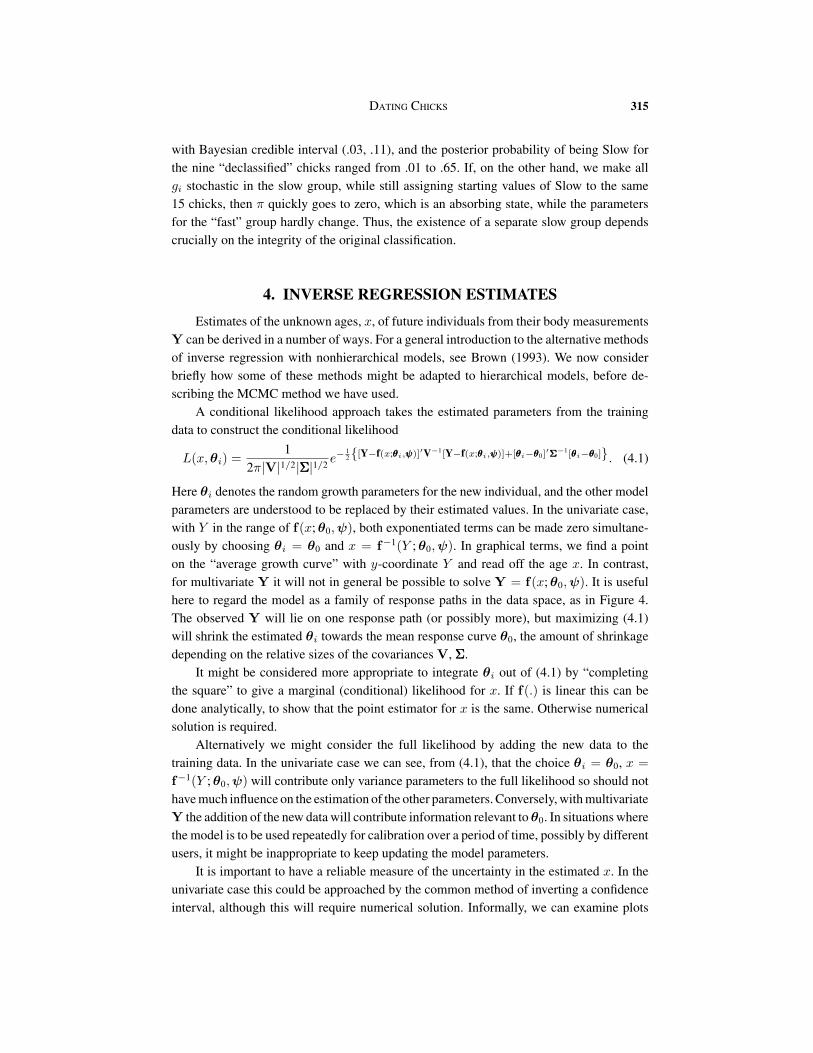
A conditional likelihood approach takes the estimated parameters from the trainingdata to construct the conditional likelihood

L(x,θi) =1

2π|V|1/2|ΣΣΣ|1/2 e−12{[Y−f(x;θθθi,ψψψ)]′V−1[Y−f(x;θθθi,ψψψ)]+[θθθi−θθθ0]′ΣΣΣ−1[θθθi−θθθ0]}. (4.1)

Here θi denotes the random growth parameters for the new individual, and the other modelparameters are understood to be replaced by their estimated values. In the univariate case,with Y in the range of f(x;θ0,ψ), both exponentiated terms can be made zero simultane-ously by choosing θi = θ0 and x = f−1(Y ;θ0,ψ). In graphical terms, we find a pointon the “average growth curve” with y-coordinate Y and read off the age x. In contrast,for multivariate Y it will not in general be possible to solve Y = f(x;θ0,ψ). It is usefulhere to regard the model as a family of response paths in the data space, as in Figure 4.The observed Y will lie on one response path (or possibly more), but maximizing (4.1)will shrink the estimated θi towards the mean response curve θ0, the amount of shrinkagedepending on the relative sizes of the covariances V, ΣΣΣ.

It might be considered more appropriate to integrate θi out of (4.1) by “completingthe square” to give a marginal (conditional) likelihood for x. If f(.) is linear this can bedone analytically, to show that the point estimator for x is the same. Otherwise numericalsolution is required.

Alternatively we might consider the full likelihood by adding the new data to thetraining data. In the univariate case we can see, from (4.1), that the choice θi = θ0, x =f−1(Y ;θ0,ψ) will contribute only variance parameters to the full likelihood so should nothavemuch influence on the estimation of the other parameters. Conversely,withmultivariateY the addition of the new data will contribute information relevant to θ0. In situations wherethe model is to be used repeatedly for calibration over a period of time, possibly by differentusers, it might be inappropriate to keep updating the model parameters.

It is important to have a reliable measure of the uncertainty in the estimated x. In theunivariate case this could be approached by the common method of inverting a confidenceinterval, although this will require numerical solution. Informally, we can examine plots


of the data to gain an impression of achievable accuracy. Suppose we have observed Wing= 100 mm in Figure 2, or Weight = 60 g in Figure 3. By drawing a horizontal line atthe observed value and reading off possible values of x, it is clear that calibration usinga univariate measurement will be very imprecise. An alternative approach to estimatingprecision would be a delta-method approximation for the variance of f(x;θ0,ψ). Again,for multivariate Y the difficulties are compounded.

Many of the above difficulties can be avoided by operating within the Bayesian frame-work we have adopted. The new data are added to the training data but with age x stochastic,so that in each iteration of the MCMC chain it is resampled from its full conditional dis-tribution p(x | Data, Model parameters). The intractability of the distributional form isovercome by using adaptive rejection sampling or Metropolis-Hastings steps within theMCMC sampler. The outputted values of x can then be regarded, after convergence, as asample from the posterior distribution p(x | Data), from which inferences can be made.A prior distribution for x must be specified. In the absence of any prior information, wehave used a uniform distribution on (0, 50). In our sample all surviving chicks had fledgedby 40 days. To illustrate the performance of the method we have chosen six hypotheticalpairs of measurements for tern chicks at various points in the data space (Figure 4), eachpair representing simultaneous measurement of wingspan and weight for a different un-known chick, and compared the posterior distributions for Wing only, Weight, and Wing +Weight. The results are summarized in Table 4 and Figure 5. It can be seen that the use oftwo measurements greatly increases the precision of the estimates, and that point estimatesusing a single measurement are often quite different. Regarding the situation graphically,we can see from Figures 2 and 3 that a single measurement gives no information about thegrowth parameters, so the posterior distributions for these, and hence for x, are very wide,especially because the individual variation around the growth curves is small compared tothe variation between curves. Considering Figure 4, in contrast, we find that bivariate infor-mation gives a point on a particular growth curve or curves, so is quite informative aboutthe new individual’s growth parameters. If Weight only is used, the posterior distributionsare very skewed because of the vertical asymptote, and here the prior constraint becomesactive.

Bivariate information can also be used for discrimination between groups. Again con-sidering Figure 4, there are regions of the data space where the slow growers should pre-dominate. If we accept that there are two groups, but that the group membership of the newchicks is unobserved, the gi nodes for these chicks can be made stochastic and resampled.This gives a posterior probability of being in each group, depending on the measurementsfor the chick and the overall group proportions. The posterior means of the probability ofbeing Slow for our hypothetical chicks were .038, .012, .113, .007, .114, .006. Thus, eventhe chicks intended, by the choice of wing length and weight, to be Slow (numbers 3 and5) were not classified as Slow. This result tends to shed further doubt on the existence of aseparate group.

We have found that there are many regions of the data space where reasonably preciseage determination can be achieved, but others where the precision is very poor. Points in the

DATING CHICKS 317

Figure 4. Simulated response paths from fitted model. The unbroken line is the mean response path θθθi = θθθ0. Theplotted points are the six hypothetical chicks used for age determination.

data space will lie not on one but on a whole family of possible response paths (see Figure4). In some areas these will tend to similar parameters and hence give similar estimates ofage. In other regions “braiding” occurs, when paths with quite different growth parametersintermesh. In such situations precise age determination will not be possible. Figure 6 showsthe posterior distributions of the growth parameters for one such region. Here the length ofthe MCMC chain was increased to 15,000 to ensure an accurate picture of the shapes of theposterior distributions. Bimodality in the weight asymptote parameter Ci is clear, and alsoprobably in the wing length growth rate Bi. The resulting poor precision in the age estimatefor Chick 3 is seen in Table 4 and Figure 5.

Table 4. Results of MCMC Estimation of Age of Unknown Chicks From BUGS1.4. Three methods areconsidered, using Wing length only, Weight only and both Wing length and Weight. Values aremean (2.5%, 97.5%) of samples of 8000 from the posterior distribution of the age (in days),after discarding an initial 4,000 values.

Wing WingGroup length (mm) Weight (g) length only Weight only Both

Fast 23 30 5.88 ( 1.91, 9.92) 6.57 ( 2.70, 17.64) 4.44 ( 3.52, 5.35)Fast 33 43 7.71 ( 3.66, 11.92) 10.32 ( 5.18, 27.21) 6.05 ( 5.23, 6.92)Slow 60 41 15.92 ( 8.90, 26.75) 20.59 ( 6.75, 47.53) 12.00 ( 8.62, 17.16)Fast 68 65 13.44 ( 8.99, 18.53) 23.57 ( 9.58, 47.95) 12.66 (11.29, 14.54)Slow 105 56 26.52 (18.92, 40.96) 29.45 (11.50, 48.88) 17.04 (15.01, 19.35)Fast 108 78 20.06 (14.96, 26.84) 30.12 (13.50, 48.89) 20.63 (19.71, 21.55)


Figure 5. BUGS1.4 output of estimated posterior distributions of the ages of six hypothetical tern chicks, basedon measurements of wing length and weight.

5. DISCUSSION

We have presented and analyzed a complex multivariate hierarchical growth modelwhich can be used to estimate the ages of new individuals. The methodology can easilyextend to situations where there are different groups within the population, and can becarried out with widely available software. It does, however, require careful modeling ofthe univariate data in order to select suitable parameterizations of appropriate growth curvemodels. This preliminary analysis might be considered to compromise to a certain extentany subsequent inference done with the full Bayesian model, but the difficulty of buildingsuch a complex model without careful examination of the data seems to us formidable.

It is a common practice when fitting such growth models to assume that the errorsincrease with age or body size. The methodology could be adapted by including a variancefunction, by transforming both sides of the growth equations, or by using Gamma in placeof normal errors. We chose not to do so here as there was no compelling evidence of het-eroscedasticity. It might also be useful to transform some of the random growth parameters

Figure 6. BUGS1.4 output of estimated posterior distributions of the growth parameters αi, βi, Ci, Bi of ahypothetical tern chick with wing length 60mm and weight 41g. The bimodality, seen particularly forCi, suggests“braiding” of the response paths at this point.

DATING CHICKS 319

to improve their normality. The posterior distributions of our Bi parameters sometimesseemed long-tailed, implying that log(Bi) might be a better candidate for normality. Wemight also want to allow for autocorrelation in the error structure, perhaps using a vectorautoregressive model. We have done this successfully for the univariate analyses, but themultivariate case presents practical difficulties and is a subject for future research.

The braiding of multivariate response paths as an explanation for the varying accu-racy of calibration or discrimination is a topic which requires further exploration. Futureresearch is aimed at characterizing the degree of braiding mathematically, so that the re-gions of the data space in which precise age determination is achievable can be mappedout quickly, without having to re-estimate the full model over a grid of points. We note toothat estimating simultaneously large numbers of hypothetical, rather than actual, chicks willdistort the model parameters because, in our methodology, they are added to the existingdata. A conditional approach, in which the parameters estimated from the training data aresubsequently held constant, might have some advantages.

Finally, we note that in our illustrative example the effects of predation and fledgingon data collection have been ignored. There are further interesting questions here, such aspredicting the age of fledging and the relationship between growth rate and predation, whichare of practical importance in the future management of black-fronted tern populations(Keedwell 2002).

ACKNOWLEDGMENTSWe thank two anonymous referees for careful reading of the manuscript and some useful suggestions and

references.

[Received September 2004. Revised April 2005.]

REFERENCES

Brown, P. J. (1993), Measurement, Regression and Calibration, Oxford: Oxford University Press.

Clarke, G. P. Y. (1992), “Inverse Estimates from a Multiresponse Model,” Biometrics, 48, 1081–1094.

Davidian, M., and Giltinan, D. M. (1995), Nonlinear Models for Repeated Measurement Data, London: Chapmanand Hall.

Diggle,A., Liang, K.-Y., and Zeger, S. L. (1994), Analysis of Longitudinal Data, Oxford: Clarendon Press.

Gilks, W. R., Richardson, S., and Spiegelhalter, D. J. (eds.) (1996), Markov Chain Monte Carlo in Practice,London: Chapman and Hall.

Goldstein, H. (1995), Multilevel Statistical Models, New York: Halsted Press.

Jaffrézic, F., and Pletcher, S. D. (2000), “Statistical Models for Estimating the Genetic Basis of RepeatedMeasuresand Other Function-Valued Traits,” Genetics, 156, 913–922.

Jones, G., and Rocke, D. M. (2001), “Analyte Identification in Multivariate Calibration,” Biometrics, 57, 571–576.

Keedwell, J. R. (2002), “Black-fronted Terns and Banded Dotterels: Causes of Mortality and Comparisons ofSurvival,” Unpublished PhD Thesis, Dept. of Ecology, Massey University, NZ.


Klaassen, M. (1994), “Growth and Energetics of Tern Chicks from Temperate and Polar Environments,” The Auk,111, 525–544.

Kirkpatrick, M., and Meyer, K. (2004), “Direct Estimation of Genetic Principal Components: Simplified Analysisof Complex Phenotypes,” Genetics, 168, 2295–2306.

Ladd, W., and Lindstrom, M. (2000), “Self Modeling for Two-Dimensional Response Curves,” Biometrics, 56,89–97.

Laird, N. M., and Ware, J. H. (1982), “Random Effects Models for Longitudinal Data,” Biometrics, 38, 963–974.

Lindstrom, M. J., and Bates, D. M. (1990), “Nonlinear Mixed Effects Models for Repeated Measures Data,”Biometrics, 46, 673–687.

Menzefricke, U. (1999), “Bayesian Prediction in Growth-Curve Models with Correlated Errors,” Test, 8, 75–93.

Palmer,M. J., Phillips, B. F., and Smith, G. T. (1991), “Application of NonlinearModels with RandomCoefficientsto Growth Data,” Biometrics, 47, 623–635.

Pinheiro, J. C., and Bates, D. M. (1995), “Approximations to the Log-likelihood Function in the Nonlinear Mixed-effects Model,” Journal of Computational and Graphical Statistics, 4, 12–35.

(2000), Mixed-Effects Models in S and S-Plus, New York: Springer-Verlag.

Pritchard, J. K., Stephens, M., and Donnelly, P. (2000), “Inference of Population Structure Using MultilocusGenotype Data,” Genetics, 155, 945–959.

Rickfels, R. E. (1973) “Petterns ofGrowth inBirds. II GrowthRate andMode ofDevelopment,” Ibis, 115, 177–201.

Robert, C. P. (1996) “Mixtures of Distributions: Inference and Estimation,” in Markov Chain Monte Carlo inPractice, eds. W. R. Gilks, S. Richardson, and D. J. Spiegelhalter, London: Chapman and Hall, pp. 441–464.

Seber, G. A. F., and Wild, C. J. (1989), Nonlinear Regression, New York: Wiley.

Spiegelhalter, D. J., Thomas, A., Best, N. G., and Gilks, W. R. (1994), “BUGS: Bayesian inference Using GibbsSampling, Version 0.30, Cambridge: Medical Research Council Biostatistics Unit.

Wolfinger, R. D. (1992), “Fitting Nonlinear Mixed Models with the New NLMIXED Procedure,” in Proceedingsof the Twenty-Fourth Annual SAS Users Group International Conference, pp. 1666–1675.

Wood, J. T. (1982), “Estimating the Age of an Animal: an Application ofMultivariate Calibration,” in Proceedingsof the 11th International Biometric Conference, pp. 117–122.

Dating chicks: Calibration and discrimination in a nonlinear multivariate hierarchical growth model

Documents

Transcript of Dating chicks: Calibration and discrimination in a nonlinear multivariate hierarchical growth model