Datex-Ohmeda S/5 Collect User's Reference Manualclin.au.dk/fileadmin/ S/5 Collect User's Reference...
103
Datex-Ohmeda S/5 Collect User's Reference Manual All specifications are subject to change without notice. Document No. 8005016 March, 2003 Datex-Ohmeda Division, Instrumentarium Corporation P.O. Box 900 FIN-00031 Datex-Ohmeda Tel. +358 10 39411 Fax +358 9 146 3310 www.datex-ohmeda.com © Instrumentarium Corp. All rights reserved.
-
Upload
trinhthuan -
Category
Documents
-
view
260 -
download
4
Transcript of Datex-Ohmeda S/5 Collect User's Reference Manualclin.au.dk/fileadmin/ S/5 Collect User's Reference...

Datex-Ohmeda S/5 Collect
User's Reference Manual
All specifications are subject to change without notice.
Document No. 8005016
March, 2003
Datex-Ohmeda Division, Instrumentarium Corporation
P.O. Box 900 FIN-00031 Datex-Ohmeda
Tel. +358 10 39411 Fax +358 9 146 3310
www.datex-ohmeda.com
© Instrumentarium Corp. All rights reserved.

Intended purpose (Indications for use)
The Datex-OhmedaTM S/5 Collect is intended to be used as a research tool for collectingdata from specified Datex-Ohmeda products. The Datex-Ohmeda S/5 Collect does notaffect the intended use of these other products.
Responsibility of the manufacturer
Datex-Ohmeda Division, Instrumentarium Corporation shall in no event be liable for anydirect, indirect, incidental, special, or consequential damages caused by this product.
Trademarks
Datex®, Ohmeda®, and other trademarks S/5, AS/3, and CS/3 are property ofInstrumentarium Corp. or its subsidiaries. All other product and company names areproperty of their respective owners.

Table of contents
i
Table of contents
1 Introduction 1–1Overview .........................................................................................................................1–1About this manual............................................................................................................1–2
Typeface conventions .................................................................................................1–2Hardware and software requirements................................................................................1–3
PC and interfacing ......................................................................................................1–3Compatible Datex-Ohmeda devices ............................................................................1–3
2 Safety precautions 2–1Notes on usage................................................................................................................2–1
3 Installation and startup 3–1Installing S/5 Collect .......................................................................................................3–1Startup and registration ...................................................................................................3–4Loading PHY files .............................................................................................................3–7Exiting the S/5 Collect .....................................................................................................3–7
4 Using S/5 Collect online 4–1Starting the online mode ..................................................................................................4–1
Online main window ...................................................................................................4–3Command buttons......................................................................................................4–4Resizing the main window ...........................................................................................4–4
Online waveforms ............................................................................................................4–5Selecting the displayed waveforms..............................................................................4–6Changing the waveform sampling interval ....................................................................4–6Changing the period of waveform display.....................................................................4–8
Online trends...................................................................................................................4–9Selecting the displayed trends ................................................................................. 4–10Auto-selection of displayed trends ........................................................................... 4–10Checking the latest numerical parameter value......................................................... 4–10Changing the trend sampling interval........................................................................ 4–11Changing the trend scale ......................................................................................... 4–11Clearing the trends .................................................................................................. 4–12
Freezing the online trends and waveforms ...................................................................... 4–12Displaying alarms ......................................................................................................... 4–12Displaying events.......................................................................................................... 4–13Saving data in .drc files ................................................................................................. 4–13Saving data in ASCII files............................................................................................... 4–14Entering and modifying notes ........................................................................................ 4–15

Datex-Ohmeda S/5 Collect
ii
Taking snapshots...........................................................................................................4–17Graphical presentation of trend and waveform snapshot data ....................................4–17Working with graphical snapshots .............................................................................4–21Numeric presentation of trend and waveform snapshot data ......................................4–23Exporting snapshot data to ASCII and Excel ...............................................................4–25
Using plug-ins ...............................................................................................................4–27Printing the current window ............................................................................................4–28Exiting the online mode..................................................................................................4–28
5 Using the S/5 Collect offline 5–1Starting the offline mode..................................................................................................5–1
Offline main window ...................................................................................................5–3Times displayed in the offline mode ............................................................................5–4
Replaying the data in offline mode ...................................................................................5–5Offline waveforms ............................................................................................................5–6
Selecting the displayed waveforms .............................................................................5–7Changing the waveform sampling interval....................................................................5–7Changing the period of waveform display.....................................................................5–7Clearing the waveforms ..............................................................................................5–7
Offline trends...................................................................................................................5–8Selecting the displayed trends ....................................................................................5–9Checking the latest numerical parameter value............................................................5–9Clearing the trends .....................................................................................................5–9Auto-selection of displayed trends ..............................................................................5–9Changing the trend sampling interval ........................................................................5–10Changing the trend scale ..........................................................................................5–10
Showing data as XY graphs.............................................................................................5–11Moving to a specific time in the offline graphs .................................................................5–14Stopping an action at a desired time ..............................................................................5–16Searching for markers....................................................................................................5–17Loading PHY files ...........................................................................................................5–17Saving data in PHY files..................................................................................................5–20Saving data in .drc files..................................................................................................5–20Saving data in ASCII files ...............................................................................................5–21
Saving selected data in an ASCII file..........................................................................5–21Saving all data in an ASCII file...................................................................................5–22
Viewing ASCII files .........................................................................................................5–22Opening a new .drc file...................................................................................................5–22Printing .........................................................................................................................5–22Taking snapshots...........................................................................................................5–22Notes............................................................................................................................5–23Using plug-ins ...............................................................................................................5–23Exiting the offline mode..................................................................................................5–23

Table of contents
iii
6 Help and troubleshooting 6–1Getting help.....................................................................................................................6–1
Getting context-sensitive help .....................................................................................6–1Displaying the manual ................................................................................................6–1Showing registration information.................................................................................6–2Displaying Datex-Ohmeda web site .............................................................................6–2Showing program information .....................................................................................6–2
Error situations ................................................................................................................6–2RS232 Communication buffer indicator bar.................................................................6–2Error messages ..........................................................................................................6–3Unexpected errors ......................................................................................................6–3
7 Editing the database configuration 7–1Parameters......................................................................................................................7–2Waveforms ......................................................................................................................7–2Time format for ASCII files ................................................................................................7–3Defining the digit field color behavior ................................................................................7–3
APPENDIX A: Using LabVIEW palettes A–1Plot Legend palette..........................................................................................................A–1Scale legend palette ........................................................................................................A–3Graph palette ..................................................................................................................A–5Cursor legend palette.......................................................................................................A–6
APPENDIX B: File formats B-1Configuration files............................................................................................................ B-1
Params.txt.................................................................................................................. B-1Waves.txt ................................................................................................................... B-6
ASCII output files ............................................................................................................. B-7Alarms.asc................................................................................................................. B-7Waves.asc ............................................................................................................... B-11Trends.asc ............................................................................................................... B-12
APPENDIX C: Plug-ins C-1

Introduction
1–1
1 Introduction
Overview
The Datex-Ohmeda S/5 Collect (later on also S/5 Collect) is a 32-bit LabVIEWapplication designed for collecting measurement data from various Datex-Ohmeda monitoring products to a PC for analysis, for example, in MicrosoftExcel.
S/5 Collect features:
— Collects trend, waveform and alarm data directly from a monitor througha PC serial interface cable, or from a monitor in the network through theDatex-Ohmeda S/5 Central, and visualizes data online and offline forresearch studies.
— Allows data collection from minutes to days.
— Both online and offline data can be saved for analysis in externalapplications, such as Excel.
— In online mode, the collected data can be saved in .drc files (DatexRecord Interface format) for further analysis in offline mode.
— Saving in ASCII format available in both modes.
— In offline mode, allows converting physiological data files archived bythe Datex-Ohmeda S/5 Central into .drc format, and back.
— You can make notes and add markers during the data collection for easyanalysis.
— Saves all configured settings, making it easy to manipulate the casesbelonging to a research study.
— Expandable with user-designed plug-ins for LabVIEW, C++ or as DLL.For general LabVIEW interface guidelines, see appropriate LabVIEWmanuals at www.ni.com.
— S/5 Collect runs under Microsoft Windows NT 4.0 or later,Windows 95/98, Windows 2000 or Windows XP.
Please read the section "Safety precautions" before using the product.

Datex-Ohmeda S/5 Collect
1–2
About this manual
This manual provides instructions for installing, registering and using the Datex-Ohmeda S/5 Collect.
The manual can be found in .pdf format on the product CD-ROM in thedirectory \Documents. This directory also contains a readme.txt file.
Typeface conventions
To help you find and interpret information easily, the manual uses consistenttext formats for certain text types:
— Command buttons are written in the following way: Cancel.
— Keyboard key names are written in the following way: Esc.
— Menu commands and names of dialog box parts (text boxes, list boxes,checkboxes) are written in bold italic typeface: Location.
— Menu access is described from top to bottom. For example, the selectionof the menu command Waves in the Snapshot menu would be shown asSnapshot - Waves.
— File names, file paths and commands are written in the following way:comm.exe.
— Messages displayed on the screen are written inside single quotes:‘Learning’.
— When referring to different sections in this manual or to other manuals,section names and manual names are enclosed in double quotes:See section “Introduction."Please refer to “Datex-Ohmeda S/5 Critical Care Monitor User’sReference Manual: Introduction."
— Cautions are displayed in the following way:
CAUTION Use only specified Datex-Ohmeda interface cables.
— Warnings are displayed in the following way:
WARNING When you connect other equipment to the monitor, always makesure that the whole combination complies with the internationalsafety standard IEC 60601-1-1 for medical electrical systemsand with the requirements of local authorities.

Introduction
1–3
Hardware and software requirements
PC and interfacing
• IBM compatible 486 or Pentium PC with a minimum of 48 MB ofmemory.
• At least 20 MB free disk space.
• Microsoft Windows NT 4.0 or later, Windows 95/98, Windows2000 or Windows XP.Use Windows NT or Windows 2000 when using network communicationto S/5 Centrals.
• Screen settings: default small font size.
• For serial communication PC serial interface cable, order code 881167.
• For network communication, a normal network cable or a cross-overcable (depending on how the Collect PC will be connected to thenetwork).
Compatible Datex-Ohmeda devices
The S/5 Collect is compatible with the following Datex-Ohmeda devices:
— AS/3, CS/3 and S/5 monitors
— Light monitor
— Cardiocap 5— In case the Collect PC will be connected to the network, Central software
S-CNET02, version 2.2 or higher, is required.
NOTE: AS/3 and Light monitor software released before 1998 are not able tosend more than one waveform at a time.
NOTE: AS/3 software released before 1995 does not work with S/5 Collect.

Safety precautions
2–1
2 Safety precautions
WARNING When you connect other equipment to the monitor, always makesure that the whole combination complies with the internationalsafety standard IEC 60601-1-1 for medical electrical systemsand with the requirements of local authorities.
Connecting the power supply cord of the PC to the wall socketmay cause the leakage current in the system to exceed the limitspecified for medical equipment. The PC shall be supplied froman additional transformer providing at least basic isolation(isolating or separating transformer).
The RS232 cable connects the PC to the monitor, and therefore indirectly to thepatient.
If you are not sure whether the safety of the system is as required, pleasecontact your local technical service personnel.
CAUTION Use only specified Datex-Ohmeda interface cables.
CAUTION Prevent accidental disconnection of all cables connected to the S/5Collect PC.
Notes on usage
• We recommend you use the PC with battery power.
• COM1 is used as a default port in the application settings for serialcommunication. We recommend you use this port.
Installation and startup
3–1
3 Installation and startup
The S/5 Collect is shipped on a CD-ROM. The installation program copies all thefiles that make up the application package in a directory of your choice.
NOTE: If you have ordered software license L-COLLECT 4, the CD-ROM containsfour program licenses. You can get up to 4 four passwords, and use theapplication on 4 PCs.
Installing S/5 Collect
NOTE: Before installing, close other Windows programs.
1. Insert the S/5 Collect CD-ROM in the CD-ROM drive.
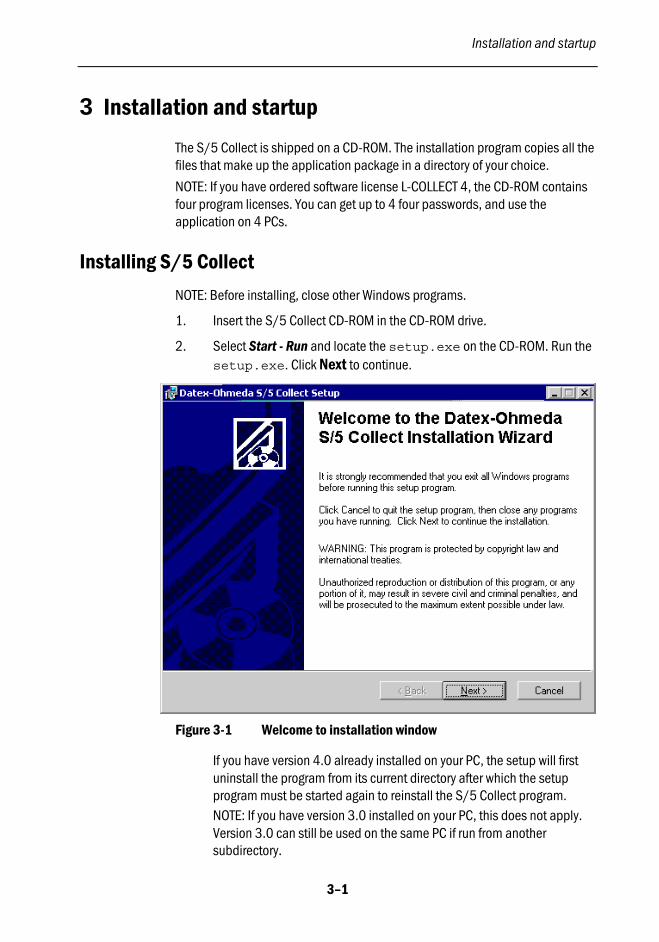
2. Select Start - Run and locate the setup.exe on the CD-ROM. Run thesetup.exe. Click Next to continue.
Figure 3-1 Welcome to installation window
If you have version 4.0 already installed on your PC, the setup will firstuninstall the program from its current directory after which the setupprogram must be started again to reinstall the S/5 Collect program.NOTE: If you have version 3.0 installed on your PC, this does not apply.Version 3.0 can still be used on the same PC if run from anothersubdirectory.

Datex-Ohmeda S/5 Collect
3–2
Figure 3-2 Uninstall window
3. If necessary, change the directory using Browse. Click Next to continue.
Figure 3-3 Setup window
Installation and startup
3–3
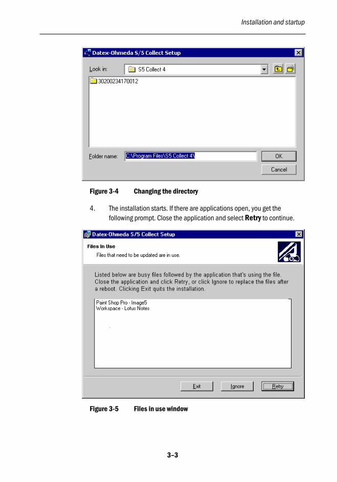
Figure 3-4 Changing the directory
4. The installation starts. If there are applications open, you get thefollowing prompt. Close the application and select Retry to continue.
Figure 3-5 Files in use window

Datex-Ohmeda S/5 Collect
3–4
5. Click Finish to complete the installation. You are prompted to restartyour computer. You can click No to continue to continue withoutrestarting.
Figure 3-6 Successful installation
The S/5 Collect entry is added in the Start menu. The installationprogram automatically installs also the LabVIEW runtime engine.
You can also access this manual in .pdf format and the readme filethrough the Start menu.
Startup and registration
1. Select Start - Programs - S5 Collect - S5 Collect. The startup window isdisplayed.

Installation and startup
3–5
Figure 3-7 Startup window
NOTE: In the startup window, you can define the path for storing the trendand wave configuration files. This enables the use of severalconfigurations for several research projects on one PC. Each newconfiguration starts with the default configuration files.
Also the paths for the latest saved ASCII file (.asc) and Datex RecordInterface file (.drc) are shown.
2. The Register button is displayed in the startup window if you have notyet registered the application.In online mode, to be able to save data in ASCII format, you need to senda registration and get a password. In offline mode, unregisteredapplications can save only 4 lines of trend data or 10 seconds ofwaveform data to ASCII files. In both modes, saving snapshots as .bmp,.jpeg and .png files is not supported if you are not registered.
Go to registering by clicking Register.
If you already have registered, continue to step 6.

Datex-Ohmeda S/5 Collect
3–6
Figure 3-8 Register dialog box
3. Get a password by sending an email or fax including the displayed PC IDand all the other information requested in the Register dialog box.
NOTE: You can use the S/5 Collect 4 on up to four PCs. To do this,register each PC separately by sending the information requested in theRegister dialog for each PC. The password is connected to the PC ID, andcannot be used on another PC. You can first register one PC, and at alater date (but within a period of 3 years) register the other PCs.
NOTE: Do not delete or change names of subdirectories in theinstallation directory of S/5 Collect. If the S/5 Collect directory and itssubdirectories are, for some reason, deleted from the hard disk, thesoftware must be registered again.
4. After receiving a password, enter it in the Password box. If the passwordis correct, the window will disappear automatically.
NOTE: If you do not have a password, you may evaluate the application,but every now and then a reminder to register will be displayed.
5. The license window is displayed. Select the I agree with all termscheckbox and click Continue.NOTE: If you do not select the I agree with all terms checkbox, theapplication will not accept your registration.
6. From the startup window, select Online or Offline.
When the program is started, the settings in the configuration file S5Collect.ini are read. This file is always saved when the program exits.
Installation and startup
3–7
Loading PHY files
You can access data that has been stored by the S/5 Central, and data on aPCMCIA card that has been used in the M-MEM module. For further informationsee "Loading PHY files" on page 5–17.
Exiting the S/5 Collect
In the main window, select File - Exit (Ctrl+Q). The S/5 Collect startup window isdisplayed. Click Exit to exit the program.

Using S/5 Collect online
4–1
4 Using S/5 Collect online
Starting the online mode1. Connect the S/5 Collect PC to the monitor through serial communication
port or to the network through Datex-Ohmeda S/5 Central.
If you use serial communication, do as follows:
• Connect the serial cable between the monitor and the PC. Themonitor should not be on while connecting the serial cable to themonitor.
• In the startup window, select Serial port and the name of the port(COM1 - COM6). COM1 is used as a default.
NOTE: Make sure that the serial cable is properly connected. If it is notproperly connected, or a wrong COM port is selected the message'Communication Timeout' will be displayed.
If you connect to a monitor through a Central, do as follows:
• If the Central is connected to the TCP/IP network, connect theCollect PC to the TCP/IP network with a normal network cable.If the Central is not connected to the TCP/IP network, connect theCollect PC to the TCP/IP network board of the Central with across-over cable.
• Specify the IP Address (192.168.1.56) and the Subnet Mask(255.255.255.0) of the Collect PC:— In Windows NT environment, right-click the Network
Neighborhood icon, select Properties, go to the Protocolstab and click the Properties button to specify the IPAddress and the Subnet Mask.
— In Windows 2000 environment, select Start - Settings-Network and Dial-up Connections and double-click theLocal Area Connection icon. Then click the Propertiesbutton, select Internet Protocol (TCP/IP) and click theProperties button to specify the IP Address and theSubnet Mask.
• For each additional Collect PC in the system, add 1 to the lastnumber of the IP address, so the second PC will be192.168.1.57, the third 192.168.1.58 and thefourth192.168.1.59. The total amount of the S/5 Collect PCsconnected in the system may not exceed 4.
Datex-Ohmeda S/5 Collect
4–2
• After specifying the IP Address and the Subnet Mask, restart theCollect PC if prompted.
• Verify that the Collect PC is connected to the Central by pingingthe Central from the DOS prompt by entering command Pingand the Computer Name of the Central.
— In Windows NT environment, select Start - Programs -Command Prompt to access the DOS prompt.
— In Windows 2000 environment, select Start - Programs -Accessories - Command Prompt to access the DOSprompt.
• In the Collect startup window, select Network Server and enterthe Computer Name of the Central to connect to. If you have morethan one Central in your system, separate the Computer Nameswith a space or a semicolon (;).
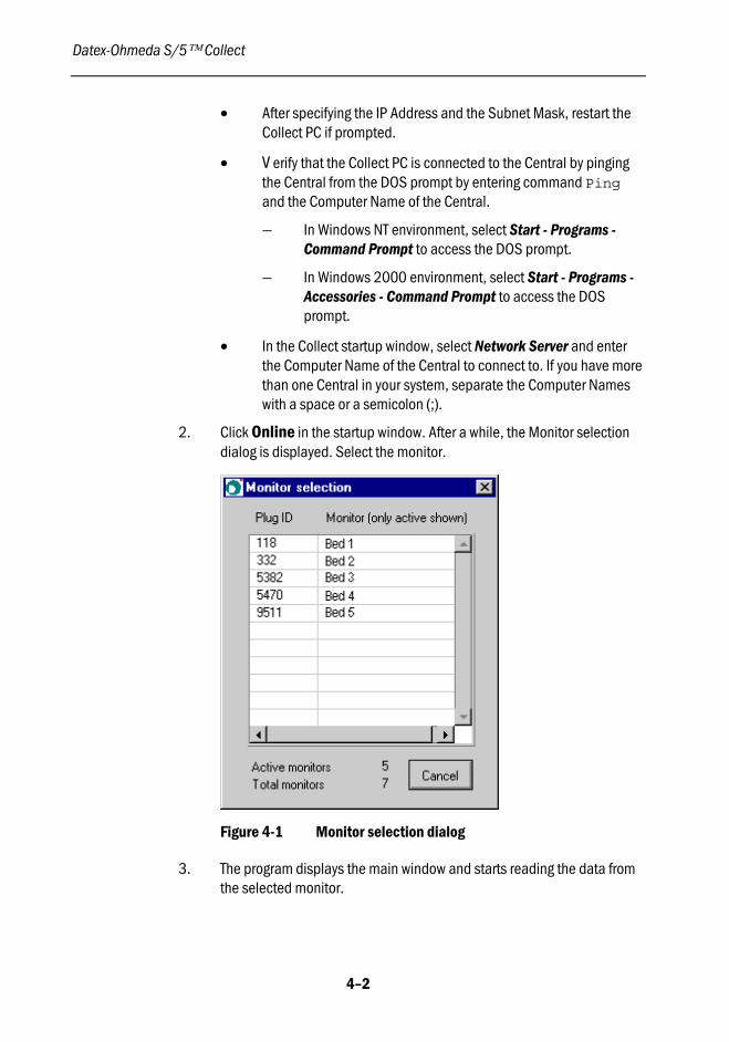
2. Click Online in the startup window. After a while, the Monitor selectiondialog is displayed. Select the monitor.
Figure 4-1 Monitor selection dialog
3. The program displays the main window and starts reading the data fromthe selected monitor.

Using S/5 Collect online
4–3
Online main window
Figure 4-2 Online main window parts
(1) Tab pages for selecting of trends and waves
(2) Command buttons
(3) Message area
(4) Available free disk space
(5) Path and name of the latest .drc or ASCII file saved
(6) Data rate in kB.
(7) A communication buffer indicator is displayed for serial communication.See "RS232 Communication buffer indicator bar," page 6–2.
(8) Current time. The time is updated every second.If you are using a network connection, the monitor id is displayed (fromthe network plug connected to the monitor, if available).
(9) Use the graph palette to scroll the display area of the graph and to zoomin and out of sections of the graph. The graph palette is available onlywhen graphs are frozen. See "Appendix A: Graph palette" for details.

Datex-Ohmeda S/5 Collect
4–4
Command buttons
Freeze stops updating the waveform and trend graphs.
DCR saves all alarm, trend and waveform data shown to a Datex RecordInterface format file (.drc) starting from the moment you press this button. Fordetails, see "Saving data in .drc files" on page 4–13.
ASCII saves alarm, trend and waveform data to separate ASCII files. The buttonis available only if DRC saving has been activated. For details, see "Saving datain ASCII files" on page 4–14.
Stop stops the current recording to a file.
Resizing the main window
You can resize the main window by selecting Window - Resize (Ctrl+S). Thismay be useful when you use, for example, Office applications on the same PCwhile collecting data.
Figure 4-3 Resized main window

Using S/5 Collect online
4–5
Online waveforms
In the main window, select the Waves page.
Figure 4-4 Online Waves page
(1) Waveforms available for selection(2) A maximum of 4 waveform boxes(3) The waveform selected to be displayed in the first waveform box. The unit
used is displayed under the selection box.(4) Use the graph palette to scroll the display area of the graph and to zoom
in and out of sections of the graph. The graph palette is available onlywhen graphs are frozen. See "Appendix A: Graph palette" for details.
(5) Waveform end time(6) Red waveform cursor. The waveform at the waveform cursor is 3 seconds
delayed from the actual waveform shown on the monitor screen.(7) Scroll bar and scroll box. By moving the scroll box you can move to the
desired part of the waveform.(8) Waveform start time
Datex-Ohmeda S/5 Collect
4–6
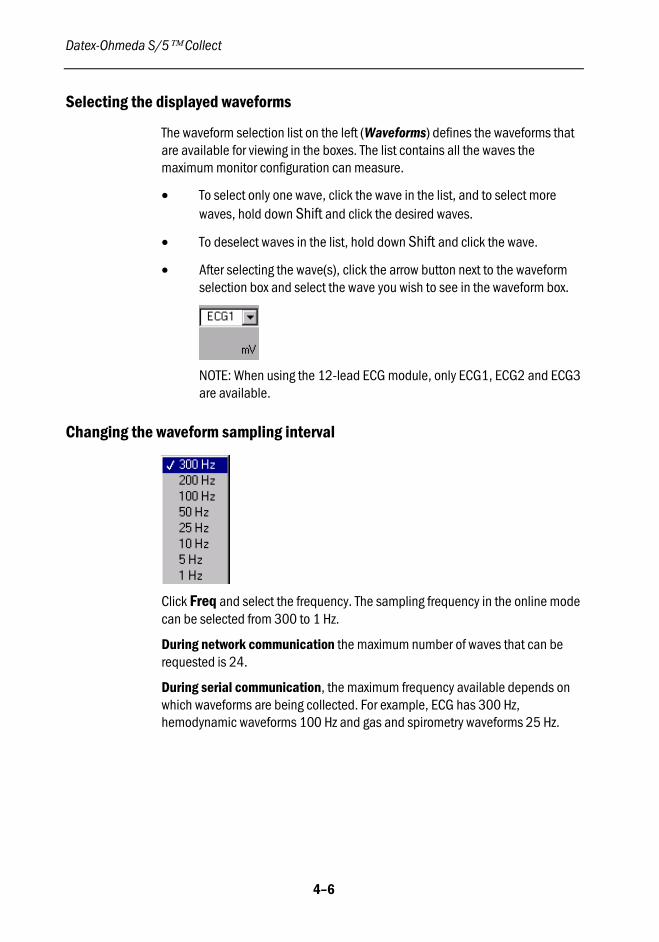
Selecting the displayed waveforms
The waveform selection list on the left (Waveforms) defines the waveforms thatare available for viewing in the boxes. The list contains all the waves themaximum monitor configuration can measure.
• To select only one wave, click the wave in the list, and to select morewaves, hold down Shift and click the desired waves.
• To deselect waves in the list, hold down Shift and click the wave.
• After selecting the wave(s), click the arrow button next to the waveformselection box and select the wave you wish to see in the waveform box.
NOTE: When using the 12-lead ECG module, only ECG1, ECG2 and ECG3are available.
Changing the waveform sampling interval
Click Freq and select the frequency. The sampling frequency in the online modecan be selected from 300 to 1 Hz.
During network communication the maximum number of waves that can berequested is 24.
During serial communication, the maximum frequency available depends onwhich waveforms are being collected. For example, ECG has 300 Hz,hemodynamic waveforms 100 Hz and gas and spirometry waveforms 25 Hz.

Using S/5 Collect online
4–7
If too many waves are selected, a prompt to reduce the amount of waveforms isdisplayed. The limit is a total of 600 samples per second; for example
2 * 300 Hz or
1 * 300 Hz + 3 * 100 Hz or
6 * 100 Hz or
2 * 100 Hz + 6 * 25 Hz or
8 * 25 Hz.
If you are collecting data from a longer period of time to an ASCII file, select alow frequency to reduce the file size.
NOTE: With certain monitor software versions, there may be a risk that thewaveform transfer is interrupted after selecting the 1 sec as the trend samplinginterval. In such case, you will also be prompted to select less waveforms.
Data file size
The table on page B-6 in "Appendix B" shows the frequency for each wave. Thevalue must be multiplied by 2 to get the number of bytes/second. The overheadeach second is 40 bytes. Trend data takes about 1500 bytes per request.
An example of asking parameters each hour for a total period of 2 days (all trendparameters are saved in the .drc file regardless of your selection):
(2 x 24) x 1500= 72 kB.
An example of collecting 2 waveforms per hour and trend data each 5 seconds:
3600 seconds 2 x InvBP waves + trend each 5 seconds =
3600 x 2 x (100 x 2 + 40) + 3600/5x1500 =
864 kB + 144 kB= 1008 kB
It is not possible to predict the exact file size of the ASCII files. The number ofcharacters in the values may make a big difference in the file size, for example, ifthe invasive pressure is 3.00 mmHg or 120.00 mmHg there are 4 or 6characters written in the file.
The online data collecting shows the file sizes while saving the data and the datarate in kB/min. From these values, you can estimate the hard disk occupationand when the saving can be made.
NOTE: The frequency selection does not affect the data transfer rate, which isalways the maximum. The data is stored in .drc files for each wave at itsindividual rate. The data is displayed and saved in ASCII files at the chosenfrequency.
Datex-Ohmeda S/5 Collect
4–8
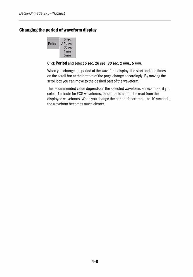
Changing the period of waveform display
Click Period and select 5 sec, 10 sec, 30 sec, 1 min., 5 min.
When you change the period of the waveform display, the start and end timeson the scroll bar at the bottom of the page change accordingly. By moving thescroll box you can move to the desired part of the waveform.
The recommended value depends on the selected waveform. For example, if youselect 1 minute for ECG waveforms, the artifacts cannot be read from thedisplayed waveforms. When you change the period, for example, to 10 seconds,the waveform becomes much clearer.

Using S/5 Collect online
4–9
Online trends
In the main window, select the Trends page.
Figure 4-5 Trends page in online mode
(1) Trends available for selection
(2) A maximum of 4 trend boxes
(3) The trend selected to be displayed in the first trend box. The latestnumerical parameter value and the unit are also displayed.
(4) Use the graph palette to scroll the display area of the graph and to zoomin and out of sections of the graph. The graph palette is available onlywhen graphs are frozen. See "Appendix A: Graph palette" for details.
(5) Trend times
The online trend data is real-time. If the PC is very slow and a lot of waves arebeing asked, trend data may also be buffered. This is indicated in thecommunication buffer indicator in the upper right corner.

Datex-Ohmeda S/5 Collect
4–10
Selecting the displayed trends
The Parameters selection list defines the parameters that are available forviewing. The list contains all parameters that the maximum monitorconfiguration can measure.
• To select only one parameter, click it.
• To select more parameters, hold down Shift and click the parameters.
• To deselect parameters in the selection list, hold down Shift and click aparameter that you wish to deselect.
• After selecting the parameters from the list, click the arrow button next tothe trend box and select the parameter you wish to see in the trend box.
Auto-selection of displayed trends
Clicking Auto Select will select and display all data with a positive valuegreater than 1 times the resolution as defined by the divider for the parametersin the configuration window.
Checking the latest numerical parameter value
The latest read numerical parameter value is shown to the right of the trend boxunder the trend selection box in a digit field. The latest read values are alsodisplayed next to the parameters in the Parameters list.

Using S/5 Collect online
4–11
Changing the trend sampling interval
Click Interval and select 1 sec, 5 sec, 10 sec, 30 sec, 1 min, 5 min, 10 min,30 min or 1 hour.
NOTE: 1 sec and 5 sec are not available during network connection.
When you want to see quick changes in the trends, select a short interval, forexample, 5 seconds. When you want to see the overall direction of the trends,select a longer interval, for example, 1 minute. If you are collecting data from along period of time, for example several hours, and have selected a shortinterval, the .drc file becomes quite large.
NOTE: With certain monitor software versions, there may be a risk that afterselecting the 1 sec trend interval, the waveform transfer is interrupted. In suchcase, you will be prompted to select less waveforms.
Changing the trend scale
Click Scale and select the desired trend time scale from values 1 min, 5 min,10 min, 20 min, 30 min, 1 hour, 2 hours, 4 hours, 6 hours, 8 hours, 12 hours,24 hours and Auto. The trend boxes start showing trends using the selectedscale. The start and end times under the trend panel change accordingly.
If you select Auto, the time scale is autoscaling all the time: the start time is thestart of the collection period, or the moment the graph was cleared last, and theend time is the time of the last package received.

Datex-Ohmeda S/5 Collect
4–12
Clearing the trends
Clicking the Clear button clears the displayed graphs and deletes the history ofeach graph.
Freezing the online trends and waveforms
If you want to stop updating both the trends and the waveforms simultaneously,press the Freeze button. Press it again to continue updating the display.
Displaying alarms
Select File - Alarms (Ctrl+A) to display all parameter alarms from the monitor.By default, the alarms are not displayed.
Figure 4-6 Alarms displayed in the online mode
NOTE: If this selection is off, the alarms are not saved in .drc and ASCII files.

Using S/5 Collect online
4–13
Displaying events
Select File -Events (available only with network communication) to display allevents from the monitor.
Events include, for example, changes in demographic data, values entered inthe calculation view, setting changes of interfaced devices, or changes in recordkeeping menus. By default, the events are not displayed.
Figure 4-7 Events displayed in the online mode.
The event is preceded by an event code and its time of occurrence. The last 100events are shown in the list.
All events will be automatically added to the notes belonging to the saved .drcfile after the online window has been closed.
Saving data in .drc files
• To start recording data in a .drc file, click the DRC button. All trend
parameters will be saved regardless of the selection. Only the selectedwaveforms will be saved (at a maximum frequency).
• To include alarm data in the .drc file, remember to first display thealarms by selecting File - Alarms (Ctrl+A). By default the alarms are notdisplayed nor saved.

Datex-Ohmeda S/5 Collect
4–14
• To include event data in the .drc file, remember to first display theevents by selecting File -Events (only available with networkcommunication).By default the events are not displayed nor saved.
• When you have clicked the DRC button, the application starts saving thedata. You will be prompted for the filename. You can see the amount ofsaved data under the DRC button.
• Click the Stop button when you have saved the desired amount of data.
Saving data in ASCII files
NOTE: This function is not available for unregistered users.NOTE: The ASCII button is available only, if DRC saving has been started.
• To start saving data in ASCII files, click ASCII. Only the selected trendsand waveforms will be saved.
• To save alarm data in an ASCII file, remember to have the File - Alarms(Ctrl+A) selection on. By default this is off.
• You will be prompted for the name of the trends file, waves file andalarms file separately. By default, file names trends.asc,waves.asc and alarms.asc are used. The waveforms will be savedat the chosen frequency.
• You can see the total size of all saved ASCII files under the ASCII button.
• When you have saved a desired amount of data, click the ASCII buttonagain. The output file formats are shown in "Appendix B: File formats".
NOTE: The decimal symbol saved in the ASCII file follows the Windows settings(Start - Settings - Control Panel - Regional Settings). Programs like MicrosoftExcel also follow this setting. When transferring the ASCII files between differentcomputers, make sure that the decimal symbol has been set the same on allcomputers.
NOTE: If you click Stop, both DRC saving and ASCII saving are stopped.

Using S/5 Collect online
4–15
Entering and modifying notes
You can enter and modify case notes by selecting Edit - Notes (Ctrl+N) in themain window. You can select notes from a predefined list, or enter notes of yourown. Here you can, for example, enter drug administrations and their effects onthe patient. The information entered in notes is first saved in a temporary .txtfile and copied to a .txt with the same root as the .drc file when the saving iscompleted. The notes can be viewed and re-edited in the offline mode.
The notes are not copied when saving only to an ASCII file.
Figure 4-8 Notes dialog box
• To select a predefined note from the list at the bottom and add it in yournotes, click the list of predefined notes, select the desired note and thenselect Edit – Add Note (F2) or click Add Note. The note is added in thelist of notes together with a timestamp.
• In the Notes window, to enter a note that is not predefined, first insert atimestamp by selecting Edit – Add Time (F1) or clicking Add Time. If youalso wish to add a date, select Edit – Add Date + Time. After this, enterthe note manually.

Datex-Ohmeda S/5 Collect
4–16
• You can generate a marker automatically by pressing the TakeSnapshot button on the patient monitor. At the next reading of theparameter data to the notes, a line is automatically added in the Casenotes with the time and the marker number.
• You can remove the contents of the Case notes by selecting File - New.
• The predefined notes are stored in notes.lst, which can be editedusing a text editor. You can add the current case notes in the selectionlist by selecting File - Store Notes - Add Case Notes to Selection List.You can replace the contents of the selection list with the current casenotes by selecting File - Store Notes - Replace Selection List with CaseNotes. All data and time stamps will be automatically removed beforethe line is made a predefined note.
• To print the Case notes shown in the Notes window, select File - Print(Ctrl+P).
• You can open a saved notes.txt file by selecting File - Open(Ctrl+O).
• You can export the note entries directly to an Excel worksheet byselecting File - Export to Excel (Ctrl+E).
Figure 4-9 File menu

Using S/5 Collect online
4–17
Taking snapshots
A snapshot contains all data in the memory (max. 30000 samples). A maximumof four parameters or waveforms can be displayed at a time. The snapshots areshown for the parameters that have been selected to be displayed in the mainwindow.
To display snapshots in the online mode, select Snapshot - Trend (Ctrl+T) orWave (Ctrl+W).
Graphical presentation of trend and waveform snapshot data
All page - snapshots off all selected waveforms or trends
Select Snapshot - Trends (Ctrl+T) or Wave (Ctrl+W) and All to show snapshotsfor all four parameters or waveforms selected to be displayed in the mainwindow. The X axis shows the time and the Y axis the parameter values.
Figure 4-10 Waveform snapshots - All snapshots page in online mode

Datex-Ohmeda S/5 Collect
4–18
Figure 4-11 Trend snapshots - All snapshots page in online mode
Overlaid page - overlaid snapshots of waveforms or trends
Select Snapshot - Trend (Ctrl+T) or Wave (Ctrl+W) and Overlaid to display asnapshot for 4 overlaid trends or waveforms at a time. You can select anddeselect each parameter from the checkboxes on the left. The X axis shows thetime and the Y axis the parameter values.
The Overlaid page is useful, for example, when you are comparing two trends orwaveforms.

Using S/5 Collect online
4–19
Figure 4-12 Waveform snapshots - Overlaid snapshots page in online mode
Figure 4-13 Trend snapshots - Overlaid snapshots page in online mode

Datex-Ohmeda S/5 Collect
4–20
One page - a snapshot of one waveform or trend
Select Snapshot - Trend (Ctrl+T) or Wave (Ctrl+W) and One to show asnapshot for one trend or waveform at a time. You can select the parameterfrom the parameter list. The X axis shows the time and the Y axis shows theparameter values.
Figure 4-14 Waveform snapshots - One snapshot page in online mode
Using S/5 Collect online
4–21
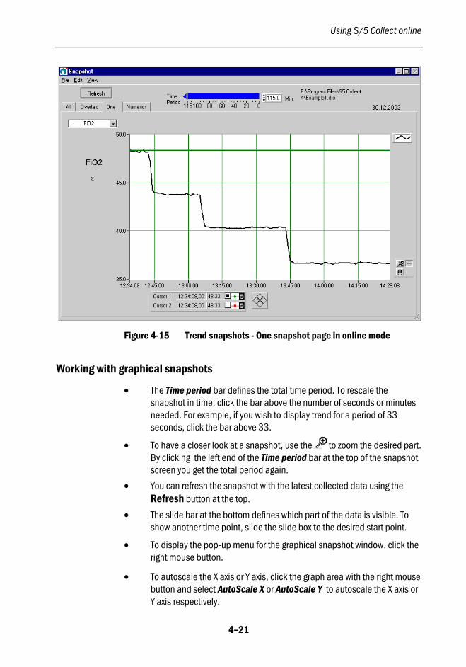
Figure 4-15 Trend snapshots - One snapshot page in online mode
Working with graphical snapshots
• The Time period bar defines the total time period. To rescale thesnapshot in time, click the bar above the number of seconds or minutesneeded. For example, if you wish to display trend for a period of 33seconds, click the bar above 33.
• To have a closer look at a snapshot, use the to zoom the desired part.By clicking the left end of the Time period bar at the top of the snapshotscreen you get the total period again.
• You can refresh the snapshot with the latest collected data using theRefresh button at the top.
• The slide bar at the bottom defines which part of the data is visible. Toshow another time point, slide the slide box to the desired start point.
• To display the pop-up menu for the graphical snapshot window, click theright mouse button.
• To autoscale the X axis or Y axis, click the graph area with the right mousebutton and select AutoScale X or AutoScale Y to autoscale the X axis orY axis respectively.

Datex-Ohmeda S/5 Collect
4–22
• You can clear the chart by selecting Clear Chart from the pop-up menu.
• To display or hide the X scale and Y scale for all of the graphssimultaneously, select Visible Items - X Scale or Y scale from the pop-up menu.
• To display a numeric data box under each the graph, select Visible Items- Digital Display from the pop-up menu. The value is the last value in theright part of the graph.
• To display or hide the scrollbar, select Visible Items - Scrollbar from thepop-up menu.
• There are several palettes available for working with the graphs. To showthem, select Visible Items form the pop-up menu and select the desiredpalette. For details about these palettes, see "Appendix A: UsingLabVIEW palettes."
• To print the currently shown snapshot page on paper on your defaultprinter, select File - Print (Ctrl+P).
• To hide the Time period bar and tab page names, select View - GraphOnly.
• To save the snapshot page in a picture file, select File - Save Graph Asand select .bmp (Ctrl+B), .png (Ctrl+J) or .jpeg (Ctrl+G). The picturefile contains same data as the paper printout. The .bmp files are big insize, .jpeg files are smaller, but may cause loss of some pixelinformation. The .png files are the smallest containing all text and lines.They can be read by most Microsoft Office applications.

Using S/5 Collect online
4–23
Numeric presentation of trend and waveform snapshot data
Select Snapshot - Trend (Ctrl+T) or Wave (Ctrl+W) and Numerics to show anumeric presentation of the data shown currently in all four trends or waveformsin the selected time period.
Figure 4-16 Waveform snapshots - Numerics page in online mode
• The Time period bar defines the total time period. To rescale thesnapshot in time, click the bar above the number of seconds or minutesneeded. For example, if you wish to display trend for a period of 33seconds, click the bar above 33.
• Click Refresh to update with the latest data collected.
• The table contains the total time period defined by the Time period barand the four parameters or waveforms selected in the main windowtogether with their values.
• The values next to the table are average, standard deviation and medianvalues of the displayed parameters.

Datex-Ohmeda S/5 Collect
4–24
• The Number of samples in average and Number of samples in medianfield can be used to filter the data in the table and all graphs in thesnapshot. Increasing Number of samples in average will apply a slidingwindow average, where the Number of samples in average is the sameas the number of samples in the window. This filter smoothens the effectof the artifacts. Increasing Number of samples in median will sort eachwindow by Number of samples in median, and pick up the middle valueof the sorted data. This filter can be used to completely rule out artifactsin the data.
• To show the currently selected table cells, click the right mouse buttonand select Show Selection from the pop-up menu.
• To hide the Time period bar, select View - Graph Only.
• To print the currently shown snapshot page on paper, select File - Print(Ctrl+P).
• To save the snapshot page in a picture file, select File - Save Graph Asand select .bmp (Ctrl+B), .png (Ctrl+J) or .jpeg (Ctrl+G). The picturefile contains same data as the paper printout. The .bmp files are big insize, .jpeg files are smaller, but may cause loss of some pixelinformation. The .png files are the smallest containing all text and lines.They can be read by most Microsoft Office applications.

Using S/5 Collect online
4–25
Exporting snapshot data to ASCII and Excel
You can save the data in the displayed snapshot to an ASCII file by selectingFile - Export Table - To ASCII (Ctrl+S).
You can save the data in the displayed snapshot to an Excel worksheet byselecting File - Export Table - To Excel (Ctrl+E). This may take a while.
Figure 4-17 Status window displayed during data transfer to Excel
Tips for using the data in Excel
• Re-edit the graph in Excel by removing or adding curves, and edit thetitles and axises before printing.
• Set the Window size in Excel to Selection to view the complete graph.You can do this by selecting View - Zoom - Fit selection.
• If the Time column includes a Date, Excel may not interpret the fieldscorrectly. In such a case, select the column and use Edit - Replace andreplace ":" with ":".
• When placing a curve on the right axis, remember to edit the order of unittexts on the Y-axis.

Datex-Ohmeda S/5 Collect
4–26
• Select graph in Excel and click the Chart Wizard icon to select, forexample, a chart type with markers or smoothing data.
• After reformatting a graph once, you can save the graph format and usethe same format again for the next graph. To do this, select Chart -Graph Type in Excel. Go to the Custom Types page and select the User-defined option button. Then click the Add button and give a name and adescription to your chart. You can set your chart to be used as the defaultchart by clicking the Set as default chart button.
Figure 4-18 Making a user-defined chart to be used as a default charttype
Using S/5 Collect online
4–27
Using plug-ins
A plug-in is a virtual LabVIEW instrument that can be modified using LabVIEW6.1. Plug-ins can be used for customizing the format of showing the collecteddata on the screen, or for performing additional calculations with the dataonline or offline.
A plug-in can run on any PC when called by the S/5 Collect without having theLabVIEW editor itself installed on the PC. The S/5 Collect uses the NI LabVIEWRunTime Engine 6.1 to run the plug-ins.
NOTE: The S/5 Collect needs to be registered to be able to run plug-ins.
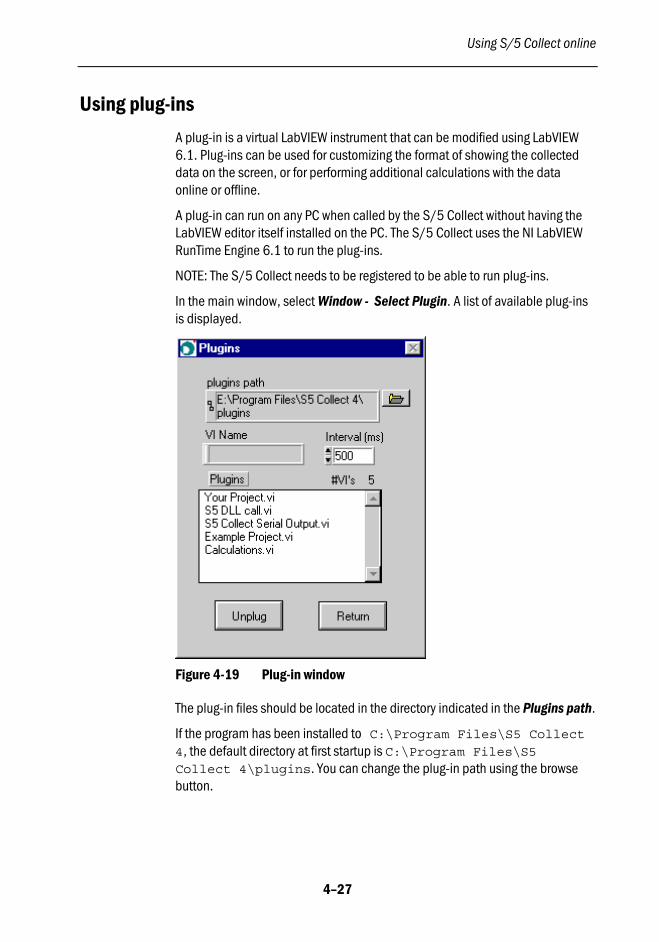
In the main window, select Window - Select Plugin. A list of available plug-insis displayed.
Figure 4-19 Plug-in window
The plug-in files should be located in the directory indicated in the Plugins path.
If the program has been installed to C:\Program Files\S5 Collect
4, the default directory at first startup is C:\Program Files\S5Collect 4\plugins. You can change the plug-in path using the browsebutton.

Datex-Ohmeda S/5 Collect
4–28
One plug-in (S5 DLL Call.vi) calls a number of functions in a .dll file(Dynamic Link Library). The sources of these functions are also located in thedefault plug-ins directory, and may be recompiled using, for example, Virtual Cto include special functions or algorithms. The results can be stored to anadditional output file for later review.
When the plug-in has been selected, the virtual LabVIEW instrument will beopened and called at regular intervals passing new data to the plug-in.
The calling interval can be changed in the online mode, see Figure 4-17 above.
The plug-in window may be reopened by selecting Window –"Plugin Name” .
See "Appendix C: Plug-ins" for information how to program plug-ins.
Printing the current window
You can print a paper copy of the current S/5 Collect window on your defaultprinter by selecting File- Print (Ctrl+P).
Exiting the online mode
In the main window, select File - Exit (Ctrl+Q) or press Esc. The S/5 Collectstartup window is displayed. Now you can exit the program, start serialcommunication or go to offline mode.

Using the S/5 Collect offline
5–1
5 Using the S/5 Collect offline
Starting the offline mode
To be able to use the S/5 Collect offline, you need to have .drc files saved inyour system.
NOTE: If you do not have any .drc files yet, and want to see how they look like,you can open one of the example .drc files, which the installation program hasinstalled in the S/5 Collect program directory. The example .drc files can alsobe found on the product CD-ROM in the directory \Patient Data.
1. Click Offline in the startup window. A window for selecting the .drc fileis displayed.
2. Select the desired .drc file and click Open.

Datex-Ohmeda S/5 Collect
5–2
The program starts replaying the first data record. After a few trend datapoints the following prompt is displayed:
Figure 5-1 Select to start playing or saving data
• To save all data in the .drc into an ASCII file without replayingthe file on the screen, select Save All to ASCII.
Trends will be saved with the trend interval that was set whilesaving to a .drc file in online mode.Waves will be saved at the previously selected frequency.
• To start replaying the data, select Start Play.
To stop the replaying, click or press F3.
• To cancel and return to the startup window, select Cancel.

Using the S/5 Collect offline
5–3
Offline main window
Figure 5-2 Example of the main window in offline mode
(1) Command buttons for replaying data, saving, taking snapshots andopening new files.
(2) Four tab pages: Trends, Waves, Trends XY and Waves XY.
(3) Name of the opened .drc file.
(4) The amount of data to read
(5) Date and time on the monitor screen, relative time, total time in the file.(See "Times displayed in the offline mode" below for details.)
(6) Use the graph palette to scroll the display area of the graph and to zoomin and out of sections of the graph. The graph palette is available onlywhen data reading has stopped. See "Appendix A: Graph palette" fordetails.

Datex-Ohmeda S/5 Collect
5–4
Times displayed in the offline mode
Figure 5-3 Times displayed in the offline mode
(1) Date and time on the monitor screen.
(2) The time relative to the start of the filebeing read.
(3) The total amount of time in the file
Figure 5-4 Example of the time bar at the bottom of the Trends page
On the Trends page, the rightmost time is the time of the last data package read.The leftmost time depends on the Scale setting. If the Scale is, for example, 10min, and the time of the last data package is 13:07:36, the leftmost time is12:57:36.
If the Scale setting is Auto, the leftmost time is the time of the first package inthe memory, or if you clicked Clear, the time of the first package after clickingClear.
Figure 5-5 Example of the time bar at the bottom of the Waves page
On the Waves page, the rightmost time under the waveform boxes is theleftmost time plus the Period setting. The red waveform cursor shows themoment of the last package received.
Using the S/5 Collect offline
5–5
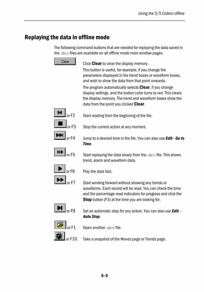
Replaying the data in offline mode
The following command buttons that are needed for replaying the data saved inthe .drc files are available on all offline mode main window pages.
Click Clear to clear the display memory.This button is useful, for example, if you change theparameters displayed in the trend boxes or waveform boxes,and wish to show the data from that point onwards.
The program automatically selects Clear, if you changedisplay settings, and the button color turns to red. This clearsthe display memory. The trend and waveform boxes show thedata from the point you clicked Clear.
or F2 Start reading from the beginning of the file.
or F3 Stop the current action at any moment.
or F4 Jump to a desired time in the file. You can also use Edit - Go toTime.
or F5 Start replaying the data slowly from the .drc file. This showstrend, alarm and waveform data.
or F6 Play the data fast.
or F7 Start winding forward without showing any trends orwaveforms. Each record will be read. You can check the timeand the percentage read indicators for progress and click theStop button (F3) at the time you are looking for.
or F9 Set an automatic stop for any action. You can also use Edit -Auto Stop.
or F1 Open another .drc file.
or F10 Take a snapshot of the Waves page or Trends page.

Datex-Ohmeda S/5 Collect
5–6
Offline waveforms
In the main window, select the Waves page.
Figure 5-6 Waves page - offline mode
(1) The Waveforms selection list defines the waveforms that are availablefor displaying in the waveform boxes.
(2) A maximum of 4 boxes for waveforms. The X axis indicates the time andthe Y axis indicates the values.
(3) You can change the waveform displayed in a particular box from thewaveform selection box.
(4) The red waveform cursor shows the moment of the last package read.
(5) Use the graph palette to scroll the display area of the graph and to zoomin and out of sections of the graph. The graph palette is available onlywhen data reading has stopped. See "Appendix A: Graph palette" fordetails.
(6) The number indicates the number of waveform records read from the file.
(7) You can move to the desired part of the waveform by moving the scrollbox.

Using the S/5 Collect offline
5–7
Selecting the displayed waveforms
• To select only one waveform, click the item in the list. To select morewaves, hold down Shift and click the desired waveforms.
• To deselect waveforms in the selection list, hold down Shift and click thewaveforms that you wish to deselect.
• After selecting the wave(s), click the arrow button next to the waveformselection box and select the wave you wish to see in the waveform box.
Changing the waveform sampling interval
Click Freq and select the frequency. The sampling frequency in the offline modecan be selected from 300 to 1 Hz. This effects the frequency shown in the offlinewindow and the frequency of samples stored to ASCII files.
Changing the period of waveform display
Click Period and select 5 sec, 10 sec, 30 sec, 1 min., 5 min.
When you change the period of the waveform display, the start time and the endtime values change accordingly on the scroll bar at the bottom. By moving thescroll box you can move to the desired part of the waveform.
The recommended period value depends on the selected waveform. Forexample, if you select 1 minute for ECG waveforms, the artifacts cannot be readfrom the displayed waveforms. When you change the period, for example, to 10seconds, the waveform becomes much clearer.
Clearing the waveforms
Click Clear to clear the displayed graphs and the display memory.
Datex-Ohmeda S/5 Collect
5–8
Offline trends
In the offline main window, select the Trends page.
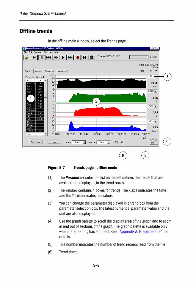
Figure 5-7 Trends page - offline mode
(1) The Parameters selection list on the left defines the trends that areavailable for displaying in the trend boxes.
(2) The window contains 4 boxes for trends. The X axis indicates the timeand the Y axis indicates the values.
(3) You can change the parameter displayed in a trend box from theparameter selection box. The latest numerical parameter value and theunit are also displayed.
(4) Use the graph palette to scroll the display area of the graph and to zoomin and out of sections of the graph. The graph palette is available onlywhen data reading has stopped. See "Appendix A: Graph palette" fordetails.
(5) This number indicates the number of trend records read from the file
(6) Trend times

Using the S/5 Collect offline
5–9
Selecting the displayed trends
1. To select only one parameter, click it. To select more parameters, holddown Shift and click the desired parameters.
2. To deselect parameters in the selection list, hold down Shift and clickthe parameter.
3. Click the arrow to the right of the parameter selection box and select the
parameter you wish to see in the trend box.
Checking the latest numerical parameter value
The latest read numerical parameter values are shown to the right of the trendbox. They are also displayed next to the Parameters selection list.
Clearing the trends
Pressing the Clear button clears the graphs and the display memory.
Auto-selection of displayed trends
Pressing Auto Select will select and display all data with a significant positivevalue after the next data has been read.

Datex-Ohmeda S/5 Collect
5–10
Changing the trend sampling interval
Click Interval and select 1 sec, 5 sec, 10 sec, 30 sec, 1 min, 5 min, 10 min,30 min or 1 hour.NOTE: 1 sec and 5 sec not available during network connection.
When you want to see quick changes in the trends, select a short interval, forexample 5 seconds. When you want to see the overall direction of the trends,select a longer interval, for example 1 minute.
Changing the trend scale
Click Scale and select the desired trend time scale from values 1 min, 5 min,10 min, 20 min, 30 min, 1 hour, 2 hours, 4 hours, 6 hours, 8 hours, 12 hours,24 hours and Auto. The trend boxes start showing trends using the selectedscale. The start and end times under the trend panel change accordingly.If you select Auto, the time scale is autoscaling all the time: the start time is thestart of the collection period, or the moment the graph was cleared last, and theend time is the time of the last package received.

Using the S/5 Collect offline
5–11
Showing data as XY graphs
You can show trend and waveform data also in an XY graph. To do this, selectthe Trends XY or Waves XY page in the main window.
For trend parameters, XY graph is an easy way to find out a correlation betweendifferent parameters. For waveforms, the XY graphs make it possible to show, forexample, spirometry loops.
Figure 5-8 Trends XY page

Datex-Ohmeda S/5 Collect
5–12
Figure 5-9 Waves XY page
You can change the displayed parameters from the parameterboxes on the left.
Change the size to have more or less history on the graph on theWaves XY page.
You can clear the graphs from the page and the display memorywith the Clear button.
You can use the cursor movement tool to move the cursor.
Use the graph palette to scroll the display area of the graph andto zoom in and out of sections of the graph. See "Appendix A:Graph palette" for details.

Using the S/5 Collect offline
5–13
Use the cursor legend palette for putting the cursor on the graph.
Figure 5-10 Cursor legend palette
(1) Cursor name
(2) Position on X axis
(3) Position on Y axis
(4) Button indicating the active cursor
(5) Cursor locking control
(6) Cursor style control
For details about the cursor legend palette, see "Appendix A: Cursor legendpalette."
Datex-Ohmeda S/5 Collect
5–14
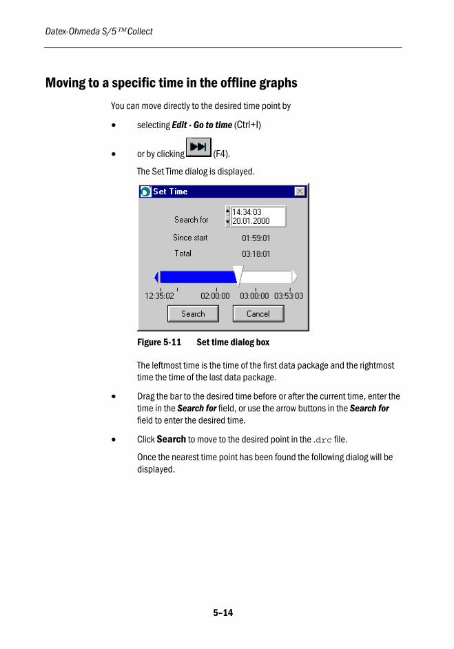
Moving to a specific time in the offline graphs
You can move directly to the desired time point by
• selecting Edit - Go to time (Ctrl+I)
• or by clicking (F4).
The Set Time dialog is displayed.
Figure 5-11 Set time dialog box
The leftmost time is the time of the first data package and the rightmosttime the time of the last data package.
• Drag the bar to the desired time before or after the current time, enter thetime in the Search for field, or use the arrow buttons in the Search forfield to enter the desired time.
• Click Search to move to the desired point in the .drc file.
Once the nearest time point has been found the following dialog will bedisplayed.

Using the S/5 Collect offline
5–15
Figure 5-12 Found. What next? dialog box
• Click Set Auto Stop Time to go directly to the dialog for setting the autostop time (see below). After leaving that dialog you will return to theFound. What next? dialog again.
• Click Start Play to start playing again at high speed. The program startsshowing graphs from the selected time onwards.
• Click Cancel to stop at the current position.
• Click Save to ASCII to save all data from the current position to theauto stop time, or if auto stop time has not been set, to the end of thefile.

Datex-Ohmeda S/5 Collect
5–16
Stopping an action at a desired time
1. To automatically stop an action at a desired time, click (F9) orselect Edit - Auto Stop (Ctrl+A). This can be used to stop any actions, forexample, playing, winding and saving.
2. Enter the desired time by entering the time in the Auto stop at box or byusing the slide bar.
3. Click Auto Stop. The auto stop time information will be shown in theupper right corner of the window. Selecting Cancel will close thiswindow and also cancel a previously set auto stop time.
4. Once the desired time is reached, the following message is displayed.Click OK.
Using the S/5 Collect offline
5–17
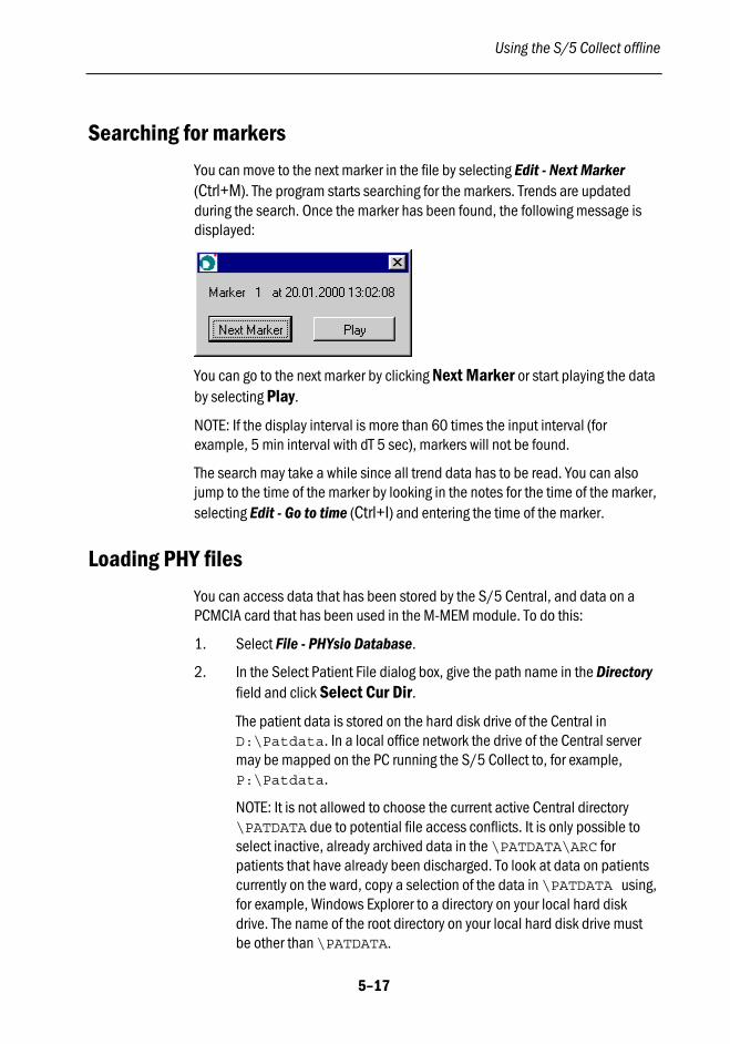
Searching for markers
You can move to the next marker in the file by selecting Edit - Next Marker(Ctrl+M). The program starts searching for the markers. Trends are updatedduring the search. Once the marker has been found, the following message isdisplayed:
You can go to the next marker by clicking Next Marker or start playing the databy selecting Play.
NOTE: If the display interval is more than 60 times the input interval (forexample, 5 min interval with dT 5 sec), markers will not be found.
The search may take a while since all trend data has to be read. You can alsojump to the time of the marker by looking in the notes for the time of the marker,selecting Edit - Go to time (Ctrl+I) and entering the time of the marker.
Loading PHY files
You can access data that has been stored by the S/5 Central, and data on aPCMCIA card that has been used in the M-MEM module. To do this:
1. Select File - PHYsio Database.
2. In the Select Patient File dialog box, give the path name in the Directoryfield and click Select Cur Dir.
The patient data is stored on the hard disk drive of the Central inD:\Patdata. In a local office network the drive of the Central servermay be mapped on the PC running the S/5 Collect to, for example,P:\Patdata.
NOTE: It is not allowed to choose the current active Central directory\PATDATA due to potential file access conflicts. It is only possible toselect inactive, already archived data in the \PATDATA\ARC forpatients that have already been discharged. To look at data on patientscurrently on the ward, copy a selection of the data in \PATDATA using,for example, Windows Explorer to a directory on your local hard diskdrive. The name of the root directory on your local hard disk drive mustbe other than \PATDATA.
Datex-Ohmeda S/5 Collect
5–18
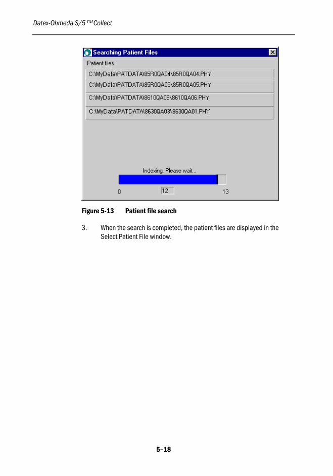
Figure 5-13 Patient file search
3. When the search is completed, the patient files are displayed in theSelect Patient File window.

Using the S/5 Collect offline
5–19
Figure 5-14 Select Patient File window showing the found files
The number of the patient files is indicated in the lower left corner of thewindow. You can sort the files by name, size, monitor ID, time, length, filename or path.
4. To convert a file to .drc format, select it and click Convert. Enter thepath in the Save as dialog box. The file is saved and opened in the offlinemode. You can select to play it or save it in ASCII format.Events stored in the patient data directory are also converted and will becopied to the notes.
You can also find examples of data that has been stored by Central on theCD-ROM in the directory \Patient Data\Central.
Datex-Ohmeda S/5 Collect
5–20
Saving data in PHY files
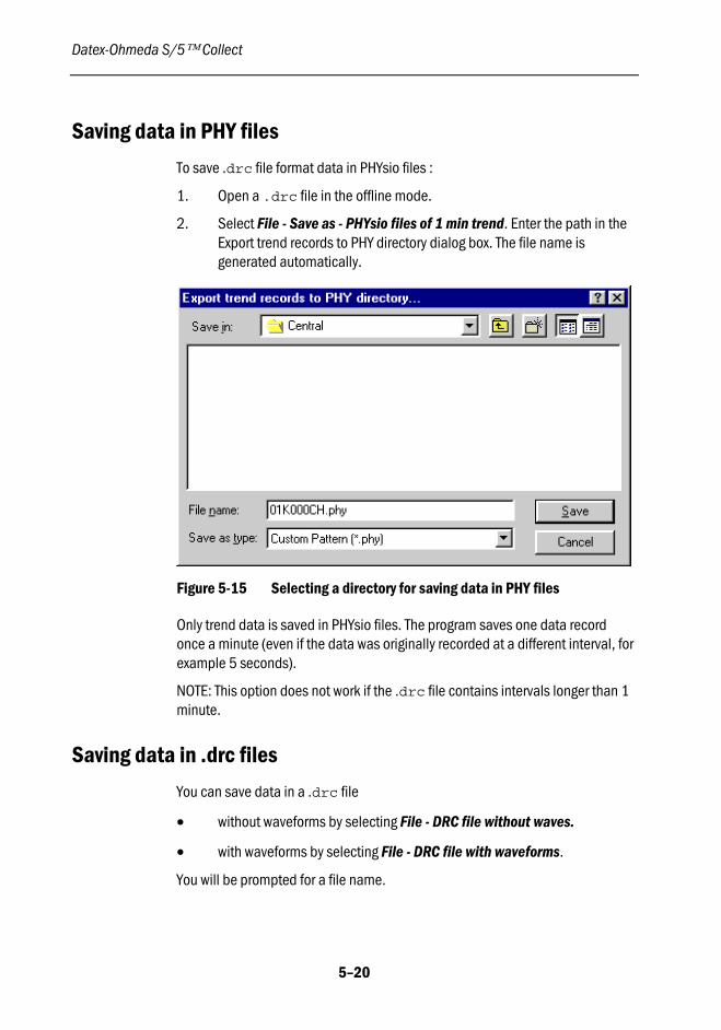
To save .drc file format data in PHYsio files :
1. Open a .drc file in the offline mode.
2. Select File - Save as - PHYsio files of 1 min trend. Enter the path in theExport trend records to PHY directory dialog box. The file name isgenerated automatically.
Figure 5-15 Selecting a directory for saving data in PHY files
Only trend data is saved in PHYsio files. The program saves one data recordonce a minute (even if the data was originally recorded at a different interval, forexample 5 seconds).
NOTE: This option does not work if the .drc file contains intervals longer than 1minute.
Saving data in .drc files
You can save data in a .drc file
• without waveforms by selecting File - DRC file without waves.
• with waveforms by selecting File - DRC file with waveforms.
You will be prompted for a file name.

Using the S/5 Collect offline
5–21
Saving data in ASCII files
Saving selected data in an ASCII file
When the desired file position is displayed, click or press F8 to startsaving the trend, waveform and alarm data in ASCII files.
• Only the selected trend and waveform parameters are saved.
• To save both trends and waveforms, click the save button while theWaves page is displayed.
• If you do not need to save waveforms in ASCII and/or want to reduce thesaving time and save only trends, click the save button while the Trendspage is displayed.
• To further reduce the saving time, select Window - Resize to hide thegraph area during saving.
• If alarm data was saved in the .drc file, it is displayed and saved toASCII.
• Data will be saved at the selected trend interval and waveformfrequency. To decrease the ASCII file size, increase the trend interval orreduce the waveform frequency.
• The selected trend scale and the period of waveform display no not haveany effect on saving, but are for displaying purposes only.
• You will be prompted for the name of the trends file, waves file andalarms file separately. By default, file names trends.asc,waves.asc and alarms.asc are used.
• To stop saving at the desired point, click or press F3.
In the ASCII files, the columns are separated by tabs. The output formats areshown in "Appendix B: File formats".
NOTE: The decimal symbol saved in the ASCII file follows the Windows settings(Start - Settings - Control Panel - Regional Settings). Programs like MicrosoftExcel also follow this setting. When transferring the ASCII files between differentPCs, make sure that the decimal symbol has been set the same on all PCs.
NOTE: Unregistered applications can save only 4 lines of trend data or 10seconds of waveform data in ASCII files.
Datex-Ohmeda S/5 Collect
5–22
Saving all data in an ASCII file
You can save all data in the .drc file in ASCII format by selecting File - Save All.You will be prompted for the file name.
NOTE: Saving all data is also possible without replaying the file on the screen.When you have started the program and selected Offline from the startupwindow, select Save All to ASCII. See page 5–2 for details.
Viewing ASCII files
Select File - View ASCII file to open a file that has been stored before as anASCII file. This selection open a *.asc or *.txt file with the default editor orviewer configured in the Windows operating system (for example Notepad).
Opening a new .drc file
At any moment, you can start working with another .drc file. To do this:
• select File - Open (Ctrl+O)
or
• click (F1).
Locate the new file and open it. The program closes the previous file and startsreading the new one.
Printing
You can print the currently displayed data on your default printer by selectingFile - Print Screen (Ctrl+ P).
Taking snapshots
You can take the snapshots
• by selecting Snapshots - Trends (Ctrl+T) or Waves (Ctrl+W)
or
• by clicking (F10).
The functionality of the snapshot pages is basically the same as in the onlinemode. See section "Taking snapshots" on page 4–17 for details.

Using the S/5 Collect offline
5–23
Notes
You can view and edit case notes by selecting Edit - Notes (Ctrl+N) in the mainoffline window. The functionality of the note editor is basically the same as in theonline mode. See section "Entering and modifying notes" on page 4–15 fordetails.
Using plug-ins
You can use the plug-ins in the same way as in the online mode. Forinstructions, see section "Using plug-ins" on page 4–27 and "Appendix C:Plug-ins."
Exiting the offline mode
In the main window, select File - Exit (Ctrl+Q) or press Esc. The S/5 Collectstartup window is displayed. Now you can exit the program, start serialcommunication or go to online mode.

Help and troubleshooting
6–1
6 Help and troubleshooting
Getting help
Figure 6-1 Help menu
Getting context-sensitive help
Selecting Help - Help displays context-sensitive help for different parts of theS/5 Collect window. The help text is displayed in a separate help panel, and thetext changes according to the cursor position.
If there is a key combination or function key connected to the function, it isindicated in the help panels. Below is an example of a help panel. In thisexample, the cursor is currently pointing the Waveforms list on the Waves page.
Figure 6-2 Example of a Context Help window
Displaying the manual
To display this manual in .pdf format, select Help - Manual. The manual canalso be found in on the product CD-ROM in the directory \Documents.
Datex-Ohmeda S/5 Collect
6–2
Showing registration information
If you have registered the application and entered your password and selectHelp - Register, the Register window with the text 'This is a registered version' isdisplayed. The password field is protected.
If you have not registered your application, a prompt for registering theapplication and entering the password is displayed.
Displaying Datex-Ohmeda web site
To go to the Datex-Ohmeda web site, select Help - Visit Web Page.
Showing program information
Selecting Help - About shows the program version and the program generationdate.
Error situations
The S/5 Collect program may be interrupted by other applications, and can runin the background. If other applications use a lot of CPU time, there is a risk thatcommunication buffers get overloaded. This may also be the case if the programis run on a slow PC (< 200 MHz Pentium).
RS232 Communication buffer indicator bar
In the upper right corner an indicator bar displays the status of the RS232communication buffers.
• The presence of a green bar indicates data has been received from themonitor but some data is being buffered. If the green bar disappears, allbuffered data has been processed.
• The size of the yellow bar indicates how much data has been read by thesoftware but not displayed on the screen yet. The data has not been fullyprocessed, usually due to too heavy CPU load. If more than 10 kB isbuffered, an overload message is displayed.
• The size of the red bar indicates how much data has been received butnot read yet at all (maximum buffer size is 30kB).

Help and troubleshooting
6–3
Error messages
If there is a communication failure between the PC and the connected Datex-Ohmeda monitor, a corresponding error message is displayed on the top.
If for some reason the data is not received intact from the connected Datex-Ohmeda monitor, a corresponding error message is displayed on the top.The error message disappears automatically when the communication restartsnormally.
Possible error messages:
Message Cause and solution
'Communication Timeout' No data received for 5 seconds. Check thecable (order number 881167). Check themonitor and make sure no other PCapplications reserve the communication port.
'Package Length Error' Package size does not correspond to headerinformation. Check that the cable is connectedproperly.
'CheckSum Error' Calculated checksum does not correspond tochecksum send with package.Check that the cable is connected properly.
Unexpected errors
If you get an unexpected error that you cannot solve yourself using thisdocumentation, please write down the error code, restart the program and tryagain. If the same error appears again, please contact the local Datex-Ohmedatechnical support and give the error code.

Editing the database configuration
7–1
7 Editing the database configuration
NOTE: The configuration does not usually need to be changed by the users. Ifyou need to add a new parameter or a waveform, please consult your Datex-Ohmeda representative.
The database configuration including the current selections is saved in theprogram directory in configuration files params.txt and waves.txt eachtime when you exit the program. See "Params.txt" and "Waves.txt" in"Appendix B" for the contents of these two files.
Select Edit - Configuration in the online or offline mode. The ConfigurationEditor is displayed.
Figure 7-1 Configuration Editor window

Datex-Ohmeda S/5 Collect
7–2
Parameters
Use the trend box or the selection box to displaythe desired parameters.
For parameters, the column, unit, description, group, position and dividersettings are given.
The value in the column indicates the label shown in parameter selection listsand ASCII files.
The description is only shown in the Configuration Editor window.
NOTE: You can change the column and description values. It may be thatadditional parameters or waveforms have been added to a monitor after therelease of this collection program. When adding new parameters, you can alsoadd data to other fields. When adding new parameters, please consult yourDatex-Ohmeda representative.
NOTE: Special caution should be taken with the group and position settings.
The monitor sends the parameter data in packages of several parameters. Agroup means the numerical code of the package of parameters the parameterbelongs to. A position refers to the parameter's position in a specific group.
The divider setting depends on the unit in use. The divider modifies the datastring given by the monitor into physiological values.
Waveforms
Use the waveform box or the selection box todisplay the desired waveforms.
For waveforms, the column, unit, description, divider, frequency, delay and filtersettings are given.
NOTE: Do not change any values in the existing fields. You may add newwaveforms in the configuration. When adding new waveforms, please consultyour Datex-Ohmeda representative.
The value in the column indicates the label shown in waveform selection listsand ASCII files.
The description is only shown in the Configuration Editor window.
The divider setting depends on the unit in use.
The frequency is defined by the monitor.

Editing the database configuration
7–3
The delays are used for synchronizing data on the screen, in the XY graphs andin the saved ASCII files. The waveform delay for gas is set to 2 seconds; this isthe default for a 3-meter sampling line. If the waves are generated bymainstream CO2 (Light Monitor), the delay should be set to 0.
If a negative number is used for the filter, it will fasten the waveform. A positivenumber will slow down the waveform.
Time format for ASCII files
The Time column in ASCII files selection box defines how the time in the timecolumn in the trend ASCII files is formatted. Absolute time in ASCII will make astring according to the Regional settings as defined in Windows Control Panel.With Relative to start the time is cumulative from the start of the time of saving.Time in unix format will use unix format in indicating the time.
Defining the digit field color behavior
The color of the digit fields on the main window Trend page indicates thestability of trend data. The color selection is affected by the value in the #Trendsamples in standard deviation calculation box. In this box, enter the numberof trend values to be included in standard deviation calculation. The numberindicates the number of samples.
Ranges for coloring the digit fields are the following:
0 to 2.5% Green
2.5 to 5% White
5 to 10% Yellow
10% or higher Red
You may use this feature to establish a steady state for selecting the moment tostart collecting data.

APPENDIX A: Using LabVIEW palettes
A–1
APPENDIX A: Using LabVIEW palettes
NOTE: The following is a modified version of the instructions given in theLabVIEW help pages. LabVIEW is a registered trademark of National InstrumentsCorporation. For more information about using LabVIEW, see LabVIEW manualsin www.ni.com.Click the right mouse button and select Visible Items.
Plot Legend palette
To display or hide the Plot Legend palette, click the right mouse button andselect Visible Items - Plot Legend. Right-click a wave in the palette to show thecommands available for formatting the plot on the screen.
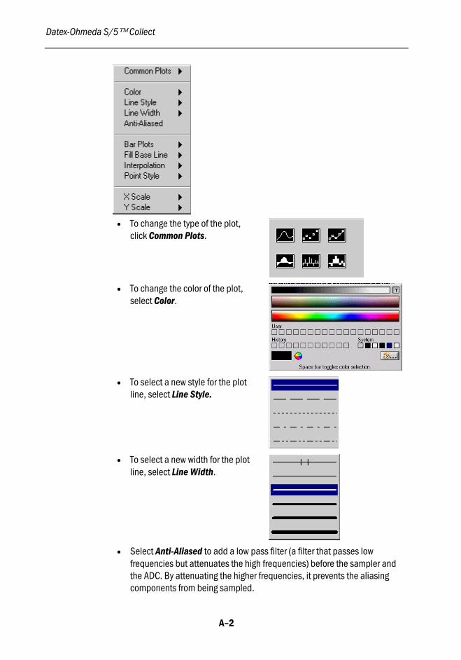
Datex-Ohmeda S/5 Collect
A–2
• To change the type of the plot,click Common Plots.
• To change the color of the plot,select Color.
• To select a new style for the plotline, select Line Style.
• To select a new width for the plotline, select Line Width.
• Select Anti-Aliased to add a low pass filter (a filter that passes lowfrequencies but attenuates the high frequencies) before the sampler andthe ADC. By attenuating the higher frequencies, it prevents the aliasingcomponents from being sampled.

APPENDIX A: Using LabVIEW palettes
A–3
• To show the data as a bar plot,select Bar Plots and the desiredbar plot style.
• To change the way the bars aredisplayed in reference to thebaseline, select Fill Base Line.
• To select the style for drawing thelines between samples, selectInterpolation.
Scale legend palette
To display or hide the Scale Legend palette, click the right mouse button andselect Visible Items - Scale Legend . With this palette, you can format the X andY scales of a graph. By using the palette, you can maintain run-time control overthe format of the X and Y scale markers respectively.
Scale Legend palette onAll snapshots page
Scale Legend palette on One snapshotspage
The first scale from the top of the palette on the All page is the X scale and thesecond is the Y scale of the first graph from the top, the third is the Y scale of thesecond graph from the top, etc.
If you want the graph to autoscale either of the scales continuously, click on thelock switch, to lock autoscaling on.
Lock switch
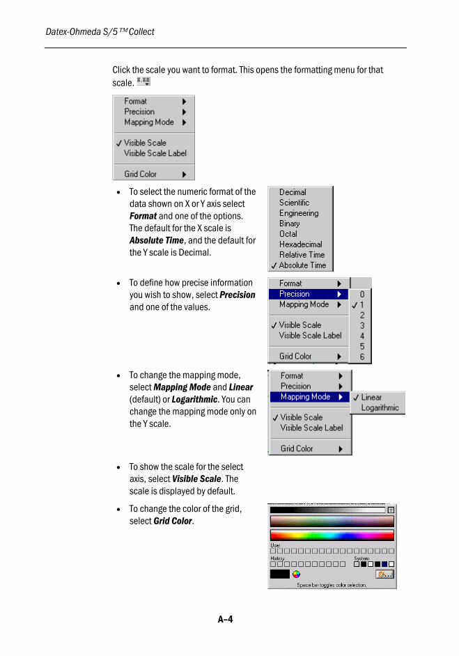
Datex-Ohmeda S/5 Collect
A–4
Click the scale you want to format. This opens the formatting menu for thatscale.
• To select the numeric format of thedata shown on X or Y axis selectFormat and one of the options.The default for the X scale isAbsolute Time, and the default forthe Y scale is Decimal.
• To define how precise informationyou wish to show, select Precisionand one of the values.
• To change the mapping mode,select Mapping Mode and Linear(default) or Logarithmic. You canchange the mapping mode only onthe Y scale.
• To show the scale for the selectaxis, select Visible Scale. Thescale is displayed by default.
• To change the color of the grid,select Grid Color.

APPENDIX A: Using LabVIEW palettes
A–5
Graph palette
To display or hide the Graph palette, click the right mouse button and selectVisible Items - Graph Palette. The Graph Palette has controls for panning(scrolling the display area of a graph) and for zooming in and out of sections ofthe graph.
Use the cursor movement tool to move the cursor on the graph.
Use the panning tool to pick up the plot and move it around on the screen.
The Zoom tool allows you to zoom in or out on the graph. If you click theZoom tool, you see a pop-up menu to choose methods of zooming.
Zoom by rectangle.
Zoom by rectangle, with zooming restricted to x data (the y scale remainsunchanged.
Zoom by rectangle, with zooming restricted to y data (the x scale remainsunchanged).
Undo last zoom. Resets the graph to its previous setting.
Zoom in about a point. If you hold down the mouse on a specific point, thegraph continuously zooms in until you release the mouse button.
Zoom out about a point. If you hold down the mouse on a specific point,the graph continuously zooms out until you release the mouse button.
NOTE: For the last two modes, zoom in and zoom out about a point, clickingShift zooms in the other direction.

Datex-Ohmeda S/5 Collect
A–6
Cursor legend palette
To display or hide the Cursor legend palette, right-click the mouse and selectVisible Items - Cursor Legend.
The Cursor palette used for putting cursors on the graph. You can label thecursor on the plot, and use a cursor as a marker. When you use a cursor as amarker, you lock the cursor to a data plot so the cursor follows the data.
Each cursor for a graph has the following parts.
The cursor label. You can change the name by entering a new namein the box.
X and Y coordinates.
A button that marks the plot for movement with the plot cursor pad.
A button that controls the look of the cursor. The following selections areavailable:
A lock control button that determines if the cursor is locked to a plot ormoved freely. The following selections are available:
Cursor movement tool.

Appendix B: File formats
B-1
APPENDIX B: File formats
Configuration files
The configuration files are located in the program directory. Each file may beedited with spreadsheet programs like Excel.
NOTE: Be very careful when adding or making changes in database definitionfiles. Before doing so, please consult your Datex-Ohmeda representative.
Params.txt
This file contains the parameter definitions.
Sel Gr Pos Div Name Unit Description2 0 3 1 HR /min Heart_Rate0 0 4 100 ST1 mm Lead1STLevel1 0 5 100 ST2 mm Lead2STLevel0 0 6 100 ST3 mm Lead3STLevel0 0 7 1 Imped. /min ImpedanceResp2 0 11 100 P1sys mmHg P1Systolic1 0 12 100 P1dia mmHg P1Diastolic1 0 13 100 P1mean mmHg P1Mean1 0 14 1 PR(P1) /min P1PulseRate1 0 18 100 P2sys mmHg P2Systolic1 0 19 100 P2dia mmHg P2Diastolic1 0 20 100 P2mean mmHg P2Mean1 0 21 1 PR(P2) /min P2PulseRate0 0 25 100 P3sys mmHg P3Systolic0 0 26 100 P3dia mmHg P3Diastolic0 0 27 100 P3mean mmHg P3Mean0 0 28 1 PR(P3) /min P3PulseRate1 0 32 100 P4sys mmHg P4Sys1 0 33 100 P4dia mmHg P4Diastolic1 0 34 100 P4mean mmHg P4Mean1 0 35 1 PR(P4) /min P4PulseRate0 0 39 100 NIBPsys mmHg NonInvBPSystolic0 0 40 100 NIBPdia mmHg NonInvBPDiastolic0 0 41 100 NIBPmean mmHg NonInvBPMean0 0 42 1 PR(NIBP) /min NonInvBPHeartRate0 0 46 100 T1 C Temperature11 0 50 100 T2 C Temperature20 0 54 100 T3 C Temperature30 0 58 100 T4 C Temperature4

Datex-Ohmeda S/5 Collect
B-2
Sel Gr Pos Div Name Unit Description0 0 62 100 SpO2 % SpO20 0 63 1 PR(SpO2) /min SpO2PulsRate0 0 64 100 SpO2_ir % InfraRedAmplitude0 0 65 100 SvO2p % SvO2(SpO2)2 0 69 100 EtCO2 % CO2EndTidal1 0 70 100 FiCO2 % CO2InspFraction1 0 71 1 RR(CO2) /min CO2RespRate1 0 72 10 Pamb mmHg AmbientPressure1 0 76 100 FeO2 % O2ExpFraction1 0 77 100 FiO2 % O2InspFraction1 0 81 100 FeN2O % N2OExpFraction0 0 82 100 FiN2O % N2OInspFraction0 0 86 100 FeAA % AgentExpFraction0 0 87 100 FiAA % AgentInspFraction0 0 88 100 MAC - AgentMacSum1 0 92 1 RR(Spiro) /min SpiroRespRate1 0 93 100 Ppeak cmH2O Ppeak1 0 94 100 PEEP cmH2O PEEP1 0 95 100 Pplat cmH2O Pplat1 0 96 10 TVinsp ml TidalVolInsp2 0 97 10 TVexp ml TidalVolExp1 0 98 100 Compl ml/cmH2O Compliance1 0 99 100 MVexp L/min MinuteVolExp1 0 103 1000 C.O. L/min CardiacOutput1 0 104 100 Tblood C BloodTemperature0 0 105 100 RVEF % RightVentrEjactFraction1 0 106 100 PCWP mmHg PulmWedgePress0 0 110 10 T1% % NMT10 0 111 10 TOF% % TrainOfFourPerc0 0 112 1 PTC - PTC1 0 113 1 HR(ECG) /min ECGhr1 0 114 1 HRmax /min HeartRateMax1 0 115 1 HRmin /min HeartRateMin0 0 119 100 SvO2 % SvO20 0 123 100 P5sys mmHg P5Systolic0 0 124 100 P5dia mmHg P5Diastolic0 0 125 100 P5mean mmHg P5Mean0 0 126 1 PR(P5) /min P5PulseRate0 0 130 100 P6sys mmHg P6Systolic0 0 131 100 P6dia mmHg P6Diastolic0 0 132 100 P6mean mmHg P6Mean0 0 133 1 PR(P6) /min P6PulseRate0 0 135 1 Marker 0x00FF Marker

Appendix B: File formats
B-3
Sel Gr Pos Div Name Unit Description1 1 3 1 HR(aECG) /min ArrhHeartRate0 1 4 1 RRt(aECG) mmHg ArrhRRTime0 1 5 1 PVC - PVC0 1 6 1 aStatus - ArrhStatus0 1 25 100 ST(I) mm ST(I)1 1 26 100 ST(II) mm ST(II)0 1 27 100 ST(III) mm ST(III)0 1 28 100 ST(AVL) mm ST(AVL)0 1 29 100 ST(AVR) mm ST(AVR)0 1 30 100 ST(V1) mm ST(V1)0 1 31 100 ST(V2) mm ST(V2)0 1 32 100 ST(V3) mm ST(V3)0 1 33 100 ST(V4) mm ST(V4)0 1 34 100 ST(V5) mm ST(V5)0 1 35 100 ST(V6) mm ST(V6)1 2 3 1 NMT(Count) - NMTcount1 2 4 1 NMT(R1) - NMTTrainResponse11 2 5 1 NMT(R2) - NMTt21 2 6 1 NMT(R3) - MMTt31 2 7 1 NMT(R4) - NMTt40 2 15 10 FEMG uV FrontalEMG0 2 16 10 Ampl1 uV Ampl10 2 17 10 SEF1 Hz Sef10 2 18 10 MF1 Hz MF10 2 19 1 Delta1 % Delta%10 2 20 1 Theta1 % Theta%10 2 21 1 Alpha1 % Alpha%10 2 22 1 Beta1 % Beta%10 2 23 1 BSR1 % BSR10 2 24 10 Ampl2 uV Ampl20 2 25 10 SEF2 Hz Sef20 2 26 10 MF2 Hz MF20 2 27 1 Delta2 % Delta%20 2 28 1 Theta2 % Theta%20 2 29 1 Alpha2 % Alpha%20 2 30 1 Beta2 % Beta%20 2 31 1 BSR2 % BSR20 2 32 10 Ampl3 uV Ampl30 2 33 10 SEF3 Hz Sef30 2 34 10 MF3 Hz MF30 2 35 1 Delta3 % Delta%30 2 36 1 Theta3 % Theta%30 2 37 1 Alpha3 % Alpha%3

Datex-Ohmeda S/5 Collect
B-4
Sel Gr Pos Div Name Unit Description0 2 38 1 Beta3 % Beta%30 2 39 1 BSR3 % BSR30 2 40 10 Ampl4 uV Ampl40 2 41 10 SEF4 Hz Sef40 2 42 10 MF4 Hz MF40 2 43 1 Delta4 % Delta%40 2 44 1 Theta4 % Theta%40 2 45 1 Alpha4 % Alpha%40 2 46 1 Beta4 % Beta%40 2 47 1 BSR4 % BSR40 2 51 1 BIS - BIS0 2 52 1 BisSQI % BisSignalQualityIndex0 2 53 1 BisEMG dB BisEMG0 2 54 1 BisSR - BisSuppRatio1 2 59 1 SE - StateEntropy1 2 60 1 RE - ResponseEntropy1 2 61 1 BSR - BSR1 3 3 10 VO2 ml/min O2consumption1 3 4 10 VCO2 ml/min CO2producution1 3 5 1 EE kcal/day EnergyExpenditure1 3 6 1000 RQ - RespQuotient1 3 10 100 PEEPi cmH2O IntrinsicPEEP1 3 11 100 Pmean cmH2O Pmean0 3 12 100 Raw cmH2O/L/s AirwayResistance1 3 13 100 MVinsp L/min MinuteVolInsp1 3 14 100 PEEPe cmH2O ExtrinsicPEEP1 3 15 100 MVspont L/min SpontMinVol0 3 16 100 I:E - RatioInspExpTime0 3 17 100 Tinsp sec InspTime1 3 18 100 Texp sec ExpTime1 3 19 100 StCompl ml/cmH2O StaticCompliance0 3 20 100 StPplat cmH2O StaticPplat0 3 21 100 StPEEPe cmH2O StaticPEEPe0 3 22 100 StPEEPi cmH2O StaticPEEPi0 3 33 100 FeBal % BalanceGasFe0 3 34 100 FiBal % BalanceGasFi0 3 38 100 PgCO2 kPa TonometryCO20 3 39 100 EtPgCO2 kPa EndTidalCO20 3 40 100 PaCO2 mmHg ArterialCO20 3 41 1 Delay sec Delay0 3 42 100 pHi pH pHi1 3 43 1 pHiDelay sec pHiDelay0 3 44 10 Pamb mmHg AmbientPressure

Appendix B: File formats
B-5
Sel Gr Pos Div Name Unit Description1 3 45 1 CPMA - CPMA1 3 49 100 MACage - AgentMACageSum0 0 1 1 Free1 - Free10 0 1 1 Free2 - Free20 0 1 1 Free3 - Free30 0 1 1 Free4 - Free40 0 1 1 Free5 - Free5

Datex-Ohmeda S/5 Collect
B-6
Waves.txt
This file contains the waveform definitions.Sel Freq. Delay Divider Filter Column Unit Description2 100 0 1 1 None - None0 300 0 100 0 ECG1 mV ECG1stLead0 300 0 100 0 ECG2 mV ECG2ndLead0 300 0 100 0 ECG3 mV ECG3rdLead0 100 0 100 0 P1 mmHg InvasiveP10 100 0 100 0 P2 mmHg InvasiveP20 100 0 100 0 P3 mmHg InvasiveP30 100 0 100 0 P4 mmHg InvasiveP40 100 0 100 0 Pleth % Plethysmogram0 25 2000 100 0 CO2 % CO20 25 2000 100 0 O2 % O20 25 2000 100 0 N2O % N2O0 25 2000 100 0 AA % AnesteticAgent0 25 500 10 0 Paw cmH2O AirwayPressure0 25 500 10 0 Flow L/min Flow0 25 0 100 0 Resp Ohm ImpedanceResp0 100 0 100 0 P5 mmHg InvasiveP50 100 0 100 0 P6 mmHg InvasiveP60 100 0 10 0 EEG1 uV EEG10 100 0 10 0 EEG2 uV EEG20 100 0 10 0 EEG3 uV EEG30 100 0 10 0 EEG4 uV EEG40 3000 0 1 0 RES0 - Res00 25 500 1 0 Vol ml Volume0 25 0 10 0 Ptono cmH2O TonometerPressure0 25 0 10 0 PawVent cmH2O PawVent0 25 0 10 0 FlowVent L/min FlowVent0 25 0 1 0 VolVent ml VolVent0 100 0 100 0 NIBPcuff mmHg NonInvCuffPress0 25 500 1 0 SpiroStatus - SpiroLoopInsp0 100 0 10 0 EP uV EvokePotential0 400 0 1 0 PlethC - PlethComposite0 100 0 10 0 Ent100 uV Entropy100Hz0 400 0 40 0 Ent400 uV Entropy400Hz0 100 0 1 0 RES1 - Res10 100 0 1 0 RES2 - Res20 100 0 1 0 RES3 - Res30 100 0 1 0 RES4 - Res40 100 0 1 0 ???? - Unknown

Appendix B: File formats
B-7
ASCII output files
Alarms.asc10:04:19 ID Prio Sound Type Priority Box1 Box2 Box3 Box4 Box510:04:56 300 1 0 Status
AlarmWhite alarm Apnea
10:05:14 300 0 0 StatusAlarm
Alarm is notactive
10:05:16 303 1 0 StatusAlarm
White alarm SpO2probe off
10:05:30 303 0 0 StatusAlarm
Alarm is notactive
10:05:46 303 1 0 StatusAlarm
White alarm SpO2probe off
10:05:50 303 0 0 StatusAlarm
Alarm is notactive
10:06:00 28 2 0 StatusAlarm
Yellow alarm Tachy
10:06:04 28 0 0 StatusAlarm
Alarm is notactive
Brady
10:06:04 27 2 0 StatusAlarm
Yellow alarm Brady
10:06:08 27 0 0 StatusAlarm
Alarm is notactive
10:06:48 524 1 0 HighLimitAlarm
White alarm EtCO2 high
10:06:54 524 0 0 HighLimitAlarm
Alarm is notactive
10:07:18 524 1 0 LowLimitAlarm
White alarm EtCO2 low
10:07:28 524 0 0 LowLimitAlarm
Alarm is notactive
10:07:58 28 2 1 StatusAlarm
Yellow alarm Tachy Resp high
10:07:58 523 1 1 HighLimitAlarm
White alarm Tachy Resp high
10:08:10 524 1 1 HighLimitAlarm
White alarm Tachy Resp high EtCO2 high
10:08:14 522 2 1 HighLimitAlarm
Yellow alarm Tachy SpO2 high Resp high EtCO2high

Datex-Ohmeda S/5 Collect
B-8
10:08:38 523 2 1 HighLimitAlarm
Yellow alarm Tachy SpO2 high Resp high EtCO2high
10:08:48 524 2 1 HighLimitAlarm
Yellow alarm Tachy SpO2 high Resp high EtCO2high
10:09:06 28 3 1 StatusAlarm
Red alarm Tachy SpO2 high Resp high EtCO2high
10:09:16 522 3 1 HighLimitAlarm
Red alarm Tachy SpO2 high Resp high EtCO2high
10:09:22 534 2 1 LowLimitAlarm
Yellow alarm Tachy SpO2 high Resp high EtCO2high
MVexp low
10:10:00 28 0 0 StatusAlarm
Alarm is notactive
FiO2 low
10:10:00 522 0 0 HighLimitAlarm
Alarm is notactive
FiO2 low
10:10:00 523 0 0 HighLimitAlarm
Alarm is notactive
FiO2 low
10:10:00 524 0 0 HighLimitAlarm
Alarm is notactive
FiO2 low
10:10:00 534 0 0 LowLimitAlarm
Alarm is notactive
FiO2 low
10:10:00 527 2 0 LowLimitAlarm
Yellow alarm FiO2 low
10:10:10 527 0 0 LowLimitAlarm
Alarm is notactive

Appendix B: File formats
B-9
Below is a list of alarm IDs and the corresponding alarms. This list may be useful for you when youare reading the alarms.asc file.
ID Alarm ID Alarm
1 Asystole 308 NIBP air leakage
2 Ventricular fibrillation 309 NIBP cuff occlusion
3 Rapid ventricular tachycardia 310 EtN2O >= 82
4 Ventricular tachycardia 311 EtAA > 3 MAC
5 Extreme bradycardia 312 No QRS detected
6 Extreme tachycardia 313 No Art pulse
7 PVC run >3 314 Transducer off
8 PVC triplet 315 Check resp cable
9 PVC couplet 316 Air leak
10 R-on-T PVC 317 Flow disconnection
11 Idioventricular rhythm 318 No P1 transducer
12 Ventricular bigeminy 319 No P2 transducer
13 Ventricular trigeminy 320 No P3 transducer
14 Frequent PVCs 321 No P4 transducer
15 Multifocal PVCs 322 No P5 transducer
16 Supraventricular tachycardia 323 No P6 transducer
17 Frequent SVCs 324 NMT alarm
18 Missing beat 325 SvO2 cable off
19 Unclassified arrhythmia 326 SvO2 poor signal
20 Noisy ECG 327 SvO2 temp error
21 Problem QRS 328 Leads off
22 Low amplitude 329 Batt low 1
23 Salvo 330 Batt low 2
24 Pacer non-functional 331 Network down 1
25 Pacer non-capture 332 Network down 2
26 New QRS 333 Network down 3
27 Bradycardia 334 Network down 4
28 Tachycardia 335 All source monitors disconnected
29 Long R-to-R interval 336 Source monitor 1 disconnected
30 R-to-R interval 337 Source monitor 2 disconnected
31 PVCs/min 338 Source monitor 3 disconnected
300 Apnea 339 Source monitor 4 disconnected
301 Apnea disconnection 340 Source monitor 5 disconnected
302 Occlusion 341 No CO2 sensor
303 SpO2 probe off 342 CO2 sensor failure
304 SpO2 check probe 343 Unspecified CO2 sensor
305 No SpO2 probe 344 CO2 adapter blocked
306 No SpO2 pulse 345 Faulty probe
307 NIBP cuff loose 346 Check NIBP
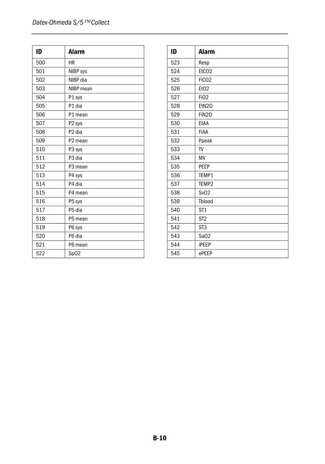
Datex-Ohmeda S/5 Collect
B-10
ID Alarm ID Alarm
500 HR 523 Resp
501 NIBP sys 524 EtCO2
502 NIBP dia 525 FiCO2
503 NIBP mean 526 EtO2
504 P1 sys 527 FiO2
505 P1 dia 528 EtN2O
506 P1 mean 529 FiN2O
507 P2 sys 530 EtAA
508 P2 dia 531 FiAA
509 P2 mean 532 Ppeak
510 P3 sys 533 TV
511 P3 dia 534 MV
512 P3 mean 535 PEEP
513 P4 sys 536 TEMP1
514 P4 dia 537 TEMP2
515 P4 mean 538 SvO2
516 P5 sys 539 Tblood
517 P5 dia 540 ST1
518 P5 mean 541 ST2
519 P6 sys 542 ST3
520 P6 dia 543 SaO2
521 P6 mean 544 iPEEP
522 SpO2 545 ePEEP

Appendix B: File formats
B-11
Waves.asc
26.01.2000 13:04:14 300 Hz 948891854ECG1 P1 Paw Flow-0,62 67,57 4,80 1,70-0,63 67,57 4,80 1,70-0,63 67,57 4,80 1,70-0,64 67,11 4,80 1,70-0,65 67,11 4,80 1,70-0,66 67,11 4,80 1,70-0,66 66,78 4,80 1,70-0,67 66,78 4,80 1,70-0,68 66,78 4,80 1,70-0,68 66,55 4,80 1,70-0,64 66,55 4,80 1,70-0,60 66,55 4,80 1,70-0,60 66,44 4,70 1,90-0,67 66,44 4,70 1,90-0,86 66,44 4,70 1,90-1,15 66,33 4,70 1,90-1,44 66,33 4,70 1,90-1,62 66,33 4,70 1,90-1,49 66,22 4,70 1,90-0,93 66,22 4,70 1,900,04 66,22 4,70 1,901,19 66,10 4,70 1,902,22 66,10 4,70 1,902,85 66,10 4,70 1,902,87 65,76 4,80 0,902,26 65,76 4,80 0,901,13 65,76 4,80 0,90-0,23 65,43 4,80 0,90-1,53 65,43 4,80 0,90-2,49 65,43 4,80 0,90-3,00 64,98 4,80 0,90-3,12 64,98 4,80 0,90

Datex-Ohmeda S/5 Collect
B-12
Trends.asc
NOTE: Values below -32000 have a special meaning:
-32764 The data exceeds lower valid limit.
-32767 There is no valid data.
-32766 Data is not updated
-32765 Data discontinuity (calibration ...).
-32764 Data exceeds lower valid limit.
-32763 Data exceeds upper valid limit.
-32762 Data is not calibrated.
-32699 Data discontinuity range end.
-32500 Data discontinuity range start.
11.12.2002 13:26:43 Trend 1039613203Time SpO2 SpO2hr CO2Et CO2rr0.00 99.00 59.00 5.06 15.008.00 99.00 55.00 5.24 15.009.00 99.00 55.00 5.24 15.0010.00 99.00 55.00 5.24 15.0011.00 99.00 55.00 5.24 15.0012.00 99.00 55.00 5.16 15.0013.00 99.00 55.00 5.16 15.0014.00 99.00 55.00 5.16 15.0015.00 99.00 56.00 5.16 15.0016.00 99.00 56.00 4.95 14.0017.00 99.00 56.00 4.95 14.0018.00 99.00 56.00 4.95 14.0019.00 99.00 56.00 4.95 14.0020.00 99.00 62.00 4.95 14.0021.00 99.00 62.00 4.95 14.0022.00 99.00 62.00 4.95 14.0023.00 99.00 62.00 4.95 14.0024.00 99.00 62.00 4.95 14.0025.00 99.00 67.00 4.95 14.0026.00 99.00 67.00 4.95 14.0027.00 99.00 67.00 4.95 14.0028.00 99.00 67.00 4.95 14.0029.00 99.00 67.00 4.95 14.00

Appendix B: File formats
B-13
30.00 99.00 62.00 4.95 14.0034.00 99.00 62.00 4.95 14.0035.00 99.00 58.00 4.95 14.0036.00 99.00 58.00 0.00 0.0037.00 99.00 58.00 0.00 0.0038.00 99.00 58.00 0.00 0.0039.00 99.00 58.00 0.00 0.0040.00 99.00 56.00 0.00 0.0041.00 99.00 56.00 0.00 0.0042.00 99.00 56.00 0.00 0.0043.00 99.00 56.00 0.00 0.0044.00 99.00 56.00 0.00 0.0045.00 99.00 54.00 0.00 0.0046.00 99.00 54.00 0.00 0.0047.00 99.00 54.00 0.00 0.0048.00 99.00 54.00 0.00 0.0049.00 99.00 54.00 0.00 0.0050.00 99.00 56.00 0.00 0.0051.00 -32767.00 -32767.00 1.11 -32767.0052.00 -32767.00 -32767.00 1.11 -32767.0053.00 -32767.00 -32767.00 1.11 -32767.0054.00 -32767.00 -32767.00 4.93 -32767.0060.00 -32767.00 -32766.00 4.54 13.0061.00 -32767.00 -32766.00 4.54 13.0062.00 -32767.00 -32766.00 4.54 13.0063.00 -32767.00 -32766.00 4.54 13.0064.00 -32767.00 -32766.00 4.54 13.0065.00 -32767.00 -32766.00 5.00 12.0066.00 -32767.00 -32766.00 5.00 12.0067.00 -32767.00 -32766.00 5.00 12.0068.00 -32767.00 -32766.00 5.00 12.0069.00 -32767.00 -32766.00 5.04 12.0070.00 -32767.00 -32766.00 5.04 12.0071.00 -32767.00 -32766.00 5.04 12.0072.00 -32767.00 -32766.00 5.04 12.0073.00 -32767.00 -32766.00 5.12 13.0074.00 -32767.00 -32766.00 5.12 13.0075.00 -32767.00 -32766.00 5.12 13.0076.00 99.00 71.00 5.12 13.0077.00 99.00 71.00 5.25 13.0078.00 99.00 71.00 5.25 13.0079.00 99.00 71.00 5.25 13.0080.00 99.50 68.00 5.25 13.0081.00 -32767.00 -32767.00 5.25 13.0082.00 -32767.00 -32767.00 4.93 13.00

Datex-Ohmeda S/5 Collect
B-14
86.00 -32767.00 -32766.00 5.39 13.0087.00 -32767.00 -32766.00 5.39 13.0088.00 -32767.00 -32766.00 5.39 13.0089.00 -32767.00 -32766.00 5.39 13.0090.00 -32767.00 -32767.00 5.34 13.0091.00 -32767.00 -32767.00 5.34 13.0092.00 -32767.00 -32767.00 5.34 13.0093.00 -32767.00 -32767.00 5.34 13.0094.00 -32767.00 -32767.00 5.36 14.0095.00 -32767.00 -32766.00 5.36 14.0096.00 -32767.00 -32766.00 5.36 14.0097.00 -32767.00 -32766.00 5.36 14.0098.00 -32767.00 -32766.00 5.28 14.00
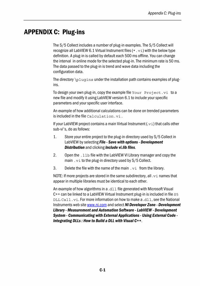
Appendix C: Plug-ins
C-1
APPENDIX C: Plug-ins
The S/5 Collect includes a number of plug-in examples. The S/5 Collect willrecognize all LabVIEW 6.1 Virtual Instrument files (*.vi) with the below typedefinition. A plug-in is called by default each 500 ms offline. You can changethe interval in online mode for the selected plug-in. The minimum rate is 50 ms.The data passed to the plug-in is trend and wave data including theconfiguration data.
The directory \plugins under the installation path contains examples of plug-ins.
To design your own plug-in, copy the example file Your Project.vi to anew file and modify it using LabVIEW version 6.1 to include your specificparameters and your specific user interface.
An example of how additional calculations can be done on trended parametersis included in the file Calculation.vi.
If your LabVIEW project contains a main Virtual Instrument (.vi) that calls othersub-vi's, do as follows:
1. Store your entire project to the plug-in directory used by S/5 Collect inLabVIEW by selecting File - Save with options - DevelopmentDistribution and clicking Include vi.lib files.
2. Open the .llb file with the LabVIEW VI Library manager and copy themain .vi to the plug-in directory used by S/5 Collect.
3. Delete the file with the name of the main .vi from the library.
NOTE: If more projects are stored in the same subdirectory, all .vi names thatappear in multiple libraries must be identical to each other.
An example of how algorithms in a .dll file generated with Microsoft VisualC++ can be linked to a LabVIEW Virtual Instrument plug-in is included in file S5DLL Call.vi. For more information on how to make a .dll, see the NationalInstruments web site www.ni.com and select NI Developer Zone - DevelopmentLibrary - Measurement and Automation Software - LabVIEW - DevelopmentSystem - Communicating with External Applications - Using External Code -Integrating DLLs : How to Build a DLL with Visual C++.

Datex-Ohmeda S/5 Collect
C-2
All C++ source files that are needed to regenerate a .dll file are copied in theplug-in directory.
When running the .vi under S/5 Collect it is possible to resize the online andoffline windows to make sufficient room to display the plug-in, while maintainingfull control over the icons and menus of the Online and Offline windows.

Appendix C: Plug-ins
C-3
Your Project.vi
Connector Pane
Front Panel

Datex-Ohmeda S/5 Collect
C-4
Controls and Indicators
Action Possible actions :0=Init : When opening the online or offline view or after selecting a new plug-inDuring init at opening of the online or offline windows only Parameters, Parameters Definitionsand Waveform Definitions are valid. All the other input parameters are equal to zero.1=Process : In the online window called each 500 ms (default) or at the interval indicated in thePlug-in selection window.In the offline window called each time a new package has been read from file. Note that duplicatedata may arrive in the plug-in. The Configuration data date-time stamp could be checked to see ifthe new package is the same as in the previous call. Alternatively the latest datex_hdr_rd could bechecked to see what the latest updated package has been before the plug-in call.During process all input variables contain valid data.2=Exit :When exiting the online or offline window the plug-in will be called with the Exit action. Thismay be used to save latest data and close the plug-in view.3=View :In the offline window called each 500 ms (default)or at the interval indicated in the Plug-in selection window. During view none of the other input variables contain valid data.Parameter Values A list of single precision values in the order indicated in the ConfigurationEditor.
Parameters A list of references to positions in the parameters list indicated in black in theselection list on the online and offline view.
Waveforms A list of references to positions in the waves list indicated in black in the selection listin the online and offline view.Waves Table
Two-dimensional array of single precision values with for each row a list of thenew samples of all selected waveforms from the last 2 seconds. The amount ofcolumns depends on the Frequency defined in the online or offline window.
Waveforms Definitions See section “Editing the database configuration.” Use this table toget all needed string constants for your plug-in.
Parameters Definitions See section “Editing the database configuration.” Use this tableto get all needed string constants for your plug-in.
Configuration Data Includes
- Information needed to set time stamps to the received trend and waveform data.
- The latest package number of the last trend and wave package.
- The time difference between the trend and wave packages (wave packages arebuffered for 3 seconds plus the maximum delay used in the Configuration window).

Appendix C: Plug-ins
C-5
Block Diagram

Datex-Ohmeda S/5 Collect
C-6

Index
Index-1
Index
A
Alarm IDs · B-11Alarms
displaying · 4–11saving in ASCII files · 4–13, 5–21saving in drc files · 4–12
Alarms.asc · B-9All page · 4–16ASCII button · 4–4, 4–13ASCII files · 4–7, 4–13, 5–2, 5–15, 5–21
decimal symbol · 4–13, 5–21output format · B-9saving data · 4–13, 5–2, 5–15, 5–21time format · 7–3total size · 4–13viewing · 5–22
ASCII output files · B-9Auto Stop · 5–16Auto Stop button · 5–5, 5–16Autoselection of trends · 4–9, 5–9
C
C++ · 1–1, 2Cancel button · 5–2, 5–15, 5–16Clear button · 4–11, 5–4, 5–5, 5–7, 5–9,
5–12Command buttons
offline mode · 5–5online mode · 4–4
Communication buffer · 4–3, 4–8overload · 6–2
Compatible Datex-Ohmeda devices · 1–3
Configuration · 7–1defining the digit field color behavior ·
7–3files · 1parameters · 7–2time format for ASCII files · 7–3waveforms · 7–2
Configuration Editor · 7–1Context-sensitive help · 6–1Convert button · 5–19Cursor legend palette · 5–13, A–6
D
Data file size · 4–7Database configuration · 7–1Datex-Ohmeda S/5 Central · 4–1, 5–17Datex-Ohmeda web site · 6–2Decimal symbol in ASCII files · 4–13, 5–21Digit field · 4–9, 5–9
defining the color behavior · 7–3Trends page · 4–9, 5–9
Displaying alarms · 4–11Displaying events · 4–12DLL · 1–1, 4–27, 2DRC button · 4–4, 4–12Drc files · 4–12, 5–1, 5–20
opening · 5–1opening a new · 5–22saving data · 4–12, 5–20selecting · 5–1
Dynamic Link Library · 4–27

Datex-Ohmeda S/5 Collect
Index-2
E
Error messages · 6–3Events
displaying · 4–12saving in drc files · 4–12
Exiting the program · 3–8Export trend records to PHY directory dialog ·
5–20
F
Found. What next? dialog · 5–15Freeze button · 4–4, 4–11
G
Go to time · 5–14Go to time button · 5–5Graph palette · A–5
H
Hardware requirements · 1–3Help menu · 6–1
I
Installation · 3–1IP address · 4–1
K
Key combinations · 6–1
L
LabVIEW · 4–26palettes · 4–21, 5–8, 5–13, A–1
LabVIEW editor · 4–26Loading PHY files · 5–17
M
Manualabout this manual · 1–2accessing through Start menu · 3–5displaying in pdf format · 6–1on CD-ROM · 1–2
Marker · 4–15searching · 5–17
Moving to a desired time · 5–14
N
NI LabVIEW RunTime Engine 6.1 · 4–26Notes · 4–14, 5–23
adding · 4–14adding markers · 4–15adding new to predefined · 4–15exporting to Excell · 4–15predefined · 4–14printing · 4–15removing contents · 4–15replacing the predefined · 4–15
Notes on usage · 2–1Numerical parameter values · 4–9, 5–9Numerics page · 4–22

Index
Index-3
O
Offline main window · 5–3Offline mode
command buttons · 5–5exiting · 5–23replaying data · 5–5starting · 5–1times displayed on screen · 5–4
One page · 4–19Online main window · 4–3
resizing · 4–4Online mode
command buttons · 4–4exiting · 4–27starting · 4–1
Open drc file button · 5–5Overlaid page · 4–17
P
Parametersconfiguration · 7–2
Params.txt · B-1Password · 3–7PCMCIA card · 5–17PHY files · 5–17
converting to drc format · 5–19saving drc data into PHY files · 5–20
Play data fast button · 5–5Play data slowly button · 5–5Plot Legend palette · A–1Plug-in · 4–26, 5–23, C-1
designing · C-1examples · C-1file location · 4–26
Predefined notes · 4–14
Printingcurrent snapshots · 4–21, 4–23current window · 4–27currently displayed data · 5–22notes · 4–15offline mode · 5–22
Program version · 6–2
R
Readme file · 1–2, 3–5Register button · 3–6Register window · 6–2Registration · 3–7, 4–13, 4–26, 5–21, 6–2Replaying data in offline mode · 5–5Resizing main window · 4–4RS232 communication buffer indicator bar ·
6–2
S
S/5 Collect · 1–1exiting · 3–8features · 1–1installing · 3–1offline mode · 5–1online mode · 4–1registering · 3–7showing version and generation date ·
6–2version 4.0 · 3–1
Safety precautions · 2–1Save All to ASCII button · 5–2, 5–22Save to ASCII button · 5–15Saving data in ASCII files · 4–13, 5–2,
5–15saving all data · 5–22saving selected data · 5–21
Saving data in drc files · 4–12, 5–20Saving data in PHY files · 5–20

Datex-Ohmeda S/5 Collect
Index-4
Scale Legend palette · A–3Searching for markers · 5–17Select Patient File dialog · 5–17, 5–18Set Auto Stop Time button · 5–15Set Time dialog · 5–14Snapshot button · 5–5Snapshots · 4–16, 5–22
All page · 4–16exporting to ASCII · 4–24exporting to Excel · 4–24Numerics page · 4–22One page · 4–19Overlaid page · 4–17printing currently displayed · 4–21, 4–23using snapshot data in Excel · 4–24working with graphical · 4–20working with numerical · 4–22
Software requirements · 1–3Start Play button · 5–2, 5–15Start reading from beginning button · 5–5Startup · 3–5
network communication · 4–1offline mode · 5–1online mode · 4–1serial communication · 4–1
Stop button · 4–4, 4–12, 4–13, 5–2, 5–5Stopping an action · 5–16
T
TCP/IP network board · 4–1Time format for ASCII files · 7–3Trends
autoselection · 4–9, 5–9clearing from screen · 4–11, 5–9configuration · 7–2freezing · 4–11
latest numerical parameter value · 4–9,5–9
sampling interval · 4–10, 5–10saving in ASCII files · 4–13, 5–2saving selected in ASCII files · 5–21selecting displayed · 4–9, 5–9showing data as XY graphs · 5–11trend scale · 4–10, 5–10
Trends page · 4–8, 5–8digit field · 4–9, 5–9
Trends XY page · 5–11Trends.asc · B-14Typeface conventions · 1–2
U
Unexpected errors · 6–3
W
Waveformsclearing · 5–7configuration · 7–2freezing · 4–11period of waveform display · 4–7, 5–7sampling interval · 4–6, 5–7saving in ASCII files · 4–13, 5–2saving selected in ASCII files · 5–21selecting displayed · 4–6, 5–7showing data as XY graphs · 5–11
Waves page · 4–5, 5–6Waves XY page · 5–11Waves.asc · B-13Waves.txt · B-7Wind forward button · 5–5Virtual Instrument · C-1Virtual LabVIEW instrument · 4–26