C:\Documents and Settings\dlfourn9\Desktop\TechMemo_TIA_DCIA_Final.doc 6/16/06

Date: May 20, 2006

To: Sarah Connick, Project Manager, Sustainable Conservation

From: Alexis Dufour, Terry Cooke

Subject: Brake Pad Partnership (BPP), Land Use Land Cover Analysis for Watershed Modeling URS Project 26814617

SUMMARY The Brake Pad Partnership (BPP) is conducting a series of interlinked environmental modeling studies to understand the transport and fate of copper from brake pad wear debris in the San Francisco Bay area. In support of the BPP’s watershed modeling effort, URS evaluated estimates of total impervious areas (TIA) and directly connected impervious area (DCIA) for use in the BPP’s watershed model, and based on BPP’s preference provided recommendations for calculating DCIA. Specifically, URS (1) compared the USGS 2001 National Land Cover Data (NLCD) TIA estimates with three local agency estimates of TIA in the San Francisco Bay area, (2) identified systematic difference between the NLCD-derived TIA and local agency estimates, and proposed a method to adjust the NLCD-derived TIA estimates to be consistent with the local agency estimates, (3) reviewed and assessed methods for calculating DCIA, (4) conducted a reality check of DCIA derived from three different methods, and (5) recommended a method for the BPP to use in calculating DCIA and the associated uncertainty values. URS found that the NLCD imperviousness layer estimates were systematically lower than local agency estimates for watersheds in the BPP study area. The difference is a constant shift of 1.5 percent for TIA between 0 and 10 percent, and of 9.6 percent for TIA greater than 10 percent. A literature review of DCIA estimation methods identified three empirical methods (Alley and Veenhuis 1983; Laenen 1983; Sutherland 1995) that could be appropriate for the BPP’s purposes. DCIA and the associated uncertainties were calculated and the results were compared to road areas and inverse parcel areas for the BPP-modeled watersheds. Empirical equations from Alley and Veenhuis (1983) and Sutherland (1995) produce similar DCIA estimates. For DCIA less than 5 percent, estimates match road surface areas. All three equations generate similar estimates between 10 and 15 percent DCIA. For DCIA greater than 10 percent, Alley and Veenhuis (1983) and Sutherland (1995) estimates are much greater than road areas, which then represent between 17 and 39 percent of the total DCIA. URS recommends the BPP use the method developed by Alley and Veenhuis (1983) to estimate DCIA as a first approximation for use in the calibration of BPP watershed model.

1.0 INTRODUCTION The Brake Pad Partnership is a multistakeholder effort to understand the impacts on the environment that may arise from brake pad wear debris generated in the use of passenger vehicles. Manufacturers, regulators, stormwater management agencies, and environmentalists are working together to understand the impacts that may arise from brake pad wear debris generated by passenger vehicles on the environment. BPP efforts are aimed at developing an approach for evaluating potential impacts of copper from brake pads affecting water quality in the South San Francisco Bay as an example. Brake pad manufacturers have committed to adding this evaluation approach to their existing practices for designing products that are safe for the environment while still meeting the performance requirements demanded of these important safety-related products. The BPP’s technical effort involves a set of interlinked laboratory, environmental monitoring, and environmental modeling studies to understand the transport and fate of copper from automobile brake pad wear debris in the environment. At the core of the BPP’s effort is three environmental modeling studies: (1) Air Deposition Modeling—to predict how much brake pad wear debris is released and deposited in the study watershed, (2) Watershed Modeling—to estimate how much copper from the deposited wear debris washes into the storm drainage system and eventually reaches the waters of the South San Francisco Bay, and (3) Bay Modeling—to determine whether and, if so, to what extent copper from brake pad wear debris affects short- and long-term concentrations of copper in the Bay. The BPP study area encompasses 23 watersheds (BPP-modeled watersheds) that drain to the San Francisco Bay (Figure 1).

Page 3 of 21

C:\Documents and Settings\dlfourn9\Desktop\TechMemo_TIA_DCIA_Final.doc 6/16/06

As described by the BPP (Sustainable Conservation 2005), several types of land use and land cover data are required to complete these modeling efforts. In the case of the watershed model (Carleton 2004), DCIA is a critical parameter. The BPP has determined that the best available data from which to derive DCIA for the purposes of the watershed modeling is the U.S. Geological Survey (USGS) 2001 NLCD (Sustainable Conservation 2005). The 2001 NLCD data are relatively up-to-date, include an imperviousness data layer, and are available for the entire study area. However, because the NLCD data are based on satellite imaging at a 30-meter resolution, the BPP is concerned that they may not account for local roads accurately, and some impervious area may be misclassified due to tree coverage (e.g., tree-lined roads). In addition, the NLCD imperviousness data layer was derived by USGS using a method that has not been verified for the San Francisco Bay area. Thus, the BPP asked URS to evaluate the 2001 NLCD data to identify the percent difference relative to local agencies’ estimates, determine whether that difference is random or systematic, and if the difference is systematic, determine how the BPP should correct for it in the watershed modeling. The BPP also asked URS to evaluate available methods for calculating DCIA and recommend the most appropriate method for the BPP to use in its watershed modeling work. DCIA estimates will be used as an initial value in the calibration of the watershed model.

2.0 ESTIMATES OF IMPERVIOUSNESS

2.1 APPROACH USGS produced imperviousness estimates using the 2001 NLCD imperviousness data layer. The data were produced using the method developed by Yang et al. (2002; MRLC 2001).1 Yang et al. tested this method in three geographic areas of varying spatial scales—Sioux Falls, South Dakota; Richmond, Virginia; and the Chesapeake Bay region. As shown in Table 1, the average error of predicted versus actual percent impervious surface ranged from 8.8 to 11.4 percent, with correlation coefficients from 0.82 to 0.91. No description of bias in error was given so it is unknown if this error was random or systematic. Given the differences in geography, vegetation, climate, and development patterns between the San Francisco Bay area and the test areas, the BPP wants to understand how the NLCD imperviousness data compare to several local agencies’ estimates of imperviousness that the BPP believes to be more accurate than the NLCD based on the degree of verification conducted using aerial photographs and site visits. URS did not review the imperviousness estimation and quality assurance methods used to determine these local estimates and followed the BPP recommendation of considering local estimates more accurate.

Table 1: Average Errors and Correlation Coefficients for the USGS Estimates of Imperviousness (Yang et al. 2002)

Area Scale Average error (percent) Correlation coefficient

Sioux Falls, South Dakota Local (~ 1,000 km2) 9.2 – 11.4 0.82 – 0.89

Richmond, Virginia Subregional (~ 10,000 km2) 8.8 – 10 0.88 – 0.91

Chesapeake Bay Regional (~ 100,000 km2) 8.8 – 10.2 0.87 – 0.90

The BPP provided URS with studies of imperviousness conducted in watersheds in three Bay Area counties—Santa Clara, San Mateo, and Alameda. In each of these studies, watershed imperviousness estimates were developed using land use data and coefficients of imperviousness per land use.2 The three sets of local agency estimates used include: • Fourteen South Bay Watersheds (EOA 2000a): Watershed impervious areas were estimated by multiplying 1995

Association of Bay Area Governments (ABAG 1996) land use areas by imperviousness coefficients within 14 watershed boundaries. Imperviousness coefficients were based on previous studies (Bredehorst 1981; EOA 1999). Some of the coefficients from both studies were evaluated by overlaying land use data on orthophotographs and digitizing impervious areas. Bredehorst (1981) found that the 95-percent confidence interval was less than +/- 8.5 percent, with average interval of +/- 3.7 percent. Impervious cover estimates per watershed were given without an uncertainty in the EOA reports.

1 Yang et al. developed an approach to estimate subpixel percent impervious surfaces at 30-meter resolution using a regression tree model with Landsat 7ETM+ data and two types of high-spatial resolution imagery (1-meter). The method employed to map percent imperviousness for NLCD 2001 consists of three key steps: deriving reference data of imperviousness from the high spatial resolution images, calibrating density prediction models using reference data and Landsat spectral bands, and extrapolating the developed models spatially to map per-pixel imperviousness. 2 A coefficient of imperviousness represents the estimated fraction of a land use that is covered by impervious surfaces.

Page 4 of 21

C:\Documents and Settings\dlfourn9\Desktop\TechMemo_TIA_DCIA_Final.doc 6/16/06

• Seventeen San Mateo County Watersheds (San Mateo Countywide Stormwater Pollution Prevention Program [STOPPP] 2002): Watershed impervious areas were estimated by multiplying ABAG land use areas by imperviousness coefficients within 17 watershed boundaries. The impervious coefficients were developed using data from previous studies (Bredehorst 1981; EOA 1997, 1998, 1999, 2000b) and data collected in the STOPPP study. For selected land uses, imperviousness coefficients were developed by digitizing impervious or pervious surfaces using high-resolution (i.e., 0.5 or 1-foot pixel resolution) orthorectified aerial photographs from 1995 or 1997. Bredehorst (1981) found that the 95-percent confidence interval was less than +/- 8.5 percent, with average interval of +/- 3.7 percent. Impervious cover estimates per watershed were given without an uncertainty in the EOA reports.

• Castro Valley Creek Watershed in Alameda County (ACPWA 1998): A detailed land use geographic information system (GIS) dataset was developed for water quality modeling (Khan 1996). The dataset was checked against high-resolution aerial photographs and field inspections. Imperviousness coefficients were assigned per land use type and were tested by calibration of the U.S. Environmental Protection Agency’s stormwater management hydrologic model. The actual estimate of impervious area was not readily available, but URS recalculated it using the same imperviousness coefficients per land use. Impervious cover estimates per watershed were given without an uncertainty in ACPWA report.

URS compared NLCD to local imperviousness estimates. Estimates were produced using different methods and possible source of differences between values are: • NLCD method is based spectral data (30-m resolution) combined with spatial imagery (1-m resolution). Canopy

coverage and impervious features smaller than the 30-m resolution can lead to misestimating imperviousness. • Local agency method used groundtruthed imperviousness coefficient and local land use data (100-m resolution). This

method assumes that imperviousness coefficient associated with a given land use does not vary among the different watersheds. The land use data has a coarse resolution but was well groundtruthed and is coded to a high specificity of land use.

2.2 METHOD URS estimated impervious areas using 2001 NLCD imperviousness layer in ArcGIS for the watersheds used in the local agencies’ studies (EOA 2000a; STOPPP 2002; ACPWA 1998). Impervious area per watershed was calculated by counting the number of pixels having the same percent imperviousness and multiplying them by the pixel area (i.e., 30 m2) to obtain the total area having the same percent imperviousness. This procedure was repeated for all percent imperviousness values and all the areas were added to obtain the TIA within a watershed. This procedure can be expressed by the following equation:

).m 30 , (i.e. area pixelunit theis

and , nessimperviouspercent with pixels ofnumber theis 10%), (e.g. nessimperviouspercent pixel theis

Area), Impervious as text in the referred (also Area Impervious Total theis Where

100

2

100

1

a

iNiTIA

aNiTIA

i

ii ××= ∑

=

Most of the watersheds in the local agencies’ reports are subwatersheds of the BPP-modeled watersheds. In these cases, the local agency watersheds were aggregated to obtain watersheds that match the corresponding BPP-modeled watershed. Comparisons were made both between the local agencies’ watersheds and between the aggregated watersheds. Local estimates were considered true values based on BPP’s recommendation.

2.3 RESULTS URS’ comparison of the 2001 NLCD imperviousness data with data developed by local agencies shows that NLCD estimates are systematically lower than local estimates. In watersheds having more than 10 percent impervious area, local agency estimates are approximately 9.6 percent greater than the NLCD estimates. In watersheds having less than 10 percent impervious area, local agency estimates are approximately 1.5 percent greater than the NLCD estimates. Comparisons of percent imperviousness estimates for the local agencies’ watersheds for which estimates are available are presented in Tables 2 and 3 and on Figure 2. None of the differences are positive showing a consistent bias of NLCD

Page 5 of 21

C:\Documents and Settings\dlfourn9\Desktop\TechMemo_TIA_DCIA_Final.doc 6/16/06

underestimating imperviousness. Comparison statistics show a systematic bias with the average difference in percent imperviousness being 12 percent (Table 3). In the Castro Valley Creek watershed, the difference between the local agency and NLCD estimates is small. While the reason for this difference is not clear, the Castro Valley Creek study included an additional step not included in the Santa Clara and San Mateo studies. In the Castro Valley Creek study the coefficients of imperviousness were tested by the calibration of a hydrologic model. This type of calibration was not conducted in the other watersheds. Regression analyses show strong trends in the data. Regressions between NLCD and local agencies’ estimates for percent imperviousness have R2 of 0.88 (Figure 2a). The slope of the regression line is greater than one indicating that NLCD estimates are lower than the local agencies’ estimates. The data points for watersheds having percent imperviousness values lower than 10 percent are somewhat separated from the main scatter of points. A separate regression for these watersheds shows a strong correlation (R2 of 0.95) and a small-unexplained error (root mean square error [RMSE] of 0.68 percent imperviousness). This regression equation has a slope of 1 and an intercept of 1.5 percent imperviousness indicating a small constant difference. The difference in percent imperviousness estimates is not correlated with watershed area and is randomly distributed around a negative mean indicating again that NLCD estimates are lower than the local agencies’ estimates. URS conducted the same comparison analysis for watersheds aggregated from the local agencies’ watersheds to match the BPP-modeled watersheds. The BPP-modeled watersheds range in size from 10.9 to 642.1 square miles, with more than half being larger than 100 square miles. This comparison was performed to develop a correction method to the systematic difference. Comparisons of impervious area and percent imperviousness estimates for the BPP-modeled watersheds for which local agencies’ estimates are available are presented in Tables 4 and 5 and on Figure 2. None of the differences are positive showing a consistent bias of NLCD underestimating total imperviousness relative to local values (Table 4). Comparison statistics show a systematic bias with the average difference in percent imperviousness being 11 percent (Table 5). Regression analyses show strong trends in the data. Regression between NLCD and local agencies’ estimates for percent imperviousness in the BPP-modeled watersheds has a R2 of 0.84 (Figure 3a). The slope of the regression line is greater than one, indicating that NLCD estimates are lower than the local agencies’ estimates. The difference between the local agencies’ and the NLCD estimates appear to be randomly distributed around a negative mean (Figure 3b). The regression equation has a slope of 1 and an intercept of 9.6 percent imperviousness, reflecting a systematic shift (Figure 3a).

Table 2: Comparison of 2001 NLCD and Local Agency Imperviousness Estimates for Watersheds in Alameda, South Bay, and Santa Clara Counties

2001 NLCD Local Agency

Watershed

URS Area (sq. mi.)

Local Agency

Area (sq. mi.)

Estimated Percent

Imperviousness (percent) Uncertainty 1

Estimated Percent

Imperviousness (percent)

∆ Estimated Percent

Imperviousness (NLCD - Local

Agency) (percent)

Castro Valley Creek 4.6 4.6 53 6 53 0 Arroyo de en Medio 1.0 1 1 0 4 -3 Sanchez Creek 1.0 1 20 2 35 -15 Mills Creek 1.2 1.2 38 4 58 -20 Belmont Creek 3.0 3 30 3 42 -12 Cordilleras Creek 3.3 3.3 20 2 35 -15 Pulgas Creek 3.5 3.5 39 4 54 -15 Denniston Creek 3.7 3.7 1 0 2 -1 Dean/Montara/San Vicente Creeks 3.9 3.9 4 1 7 -3 San Bruno Creek 3.9 3.9 44 5 51 -7

Page 6 of 21

C:\Documents and Settings\dlfourn9\Desktop\TechMemo_TIA_DCIA_Final.doc 6/16/06

Table 2: Comparison of 2001 NLCD and Local Agency Imperviousness Estimates for Watersheds in Alameda, South Bay, and Santa Clara Counties

2001 NLCD Local Agency

Watershed

URS Area (sq. mi.)

Local Agency

Area (sq. mi.)

Estimated Percent

Imperviousness (percent) Uncertainty 1

Estimated Percent

Imperviousness (percent)

∆ Estimated Percent

Imperviousness (NLCD - Local

Agency) (percent)

Frenchmans Creek 4.3 4.3 1 0 2 -1 San Mateo Creek (below Crystal Springs dam) 4.5 4.5 26 3 38 -12 Laurel Creek 4.6 4.6 40 5 53 -13 Redwood Creek 9.8 9.8 36 4 55 -19 Colma Creek 16.1 16.1 43 5 50 -7 Pilarcitos Creek 28.7 28.7 2 0 4 -2 San Francisquito Creek 42.8 42.8 7 1 21 -14 Adobe 11.3 11.3 20 2 45 -24 Arroyo la Laguna 74.4 74.4 29 3 35 -6 Baylands 32.1 32.8 19 2 25 -6 Calabazas 20.9 20.9 46 5 70 -24 Coyote 320.5 320.5 9 1 11 -2 Guadalupe 170.2 170.2 25 3 37 -12 Lower Penitencia 28.6 28.6 34 4 43 -9 Matadero/Barron 17.0 16.9 28 3 60 -32 Permanente 17.3 17.3 22 2 44 -22 San Francisquito 42.8 42.8 7 1 21 -14 San Tomas 44.8 44.8 35 4 60 -25 Stevens 29.2 29.2 17 2 29 -11 Sunnyvale East 7.1 7.1 61 7 82 -22 Sunnyvale West 7.6 7.6 56 6 72 -16 Legend Castro Valley (ACCWP) San Mateo (STOPPP) South Bay (SCVURPPP)

Notes: 1 Uncertainty was estimated at 11.4 percent based on Yang et al. (2002).

Table 3: Comparison Statistics of 2001 NLCD and Local Agency Imperviousness Estimates for Watersheds in Alameda, San Mateo, and Santa Clara Counties

Difference in Estimated Percent Imperviousness (NLCD - Local Agency)

(percent) Average -12

Minimum -32 Maximum 0

Page 7 of 21

C:\Documents and Settings\dlfourn9\Desktop\TechMemo_TIA_DCIA_Final.doc 6/16/06

Figure 2: Comparison of 2001 NLCD and Local Agency Impervious Area and Percent Imperviousness Estimates for Watersheds in Alameda, San Mateo, and Santa Clara Counties a) Correlation plot for percent imperviousness estimates b) Difference in percent imperviousness as a function of the watershed area

a)

b)

Difference in Percent Imperviousness Estimates(2001 NLCD - Local Agency)

-35

-30

-25

-20

-15

-10

-5

0

0 50 100 150 200 250 300 350

Watershed Area (sq.mi.)

Diff

. Per

cent

Imp.

(%)

Percent Imperviousness EstimatesCorrelation Plot

y = 1.201x + 7.0431R2 = 0.8779

RMSE=7.539

y = 1.0971x + 1.5494R2 = 0.9545

RMSE = 0.6800

102030405060708090

100

0 10 20 30 40 50 60 70 80 90 100

2001 NLCD Percent Imperviousness (%)

Loca

l Age

ncy

Perc

ent

Impe

rvio

usne

ss

(%)

Page 8 of 21

C:\Documents and Settings\dlfourn9\Desktop\TechMemo_TIA_DCIA_Final.doc 6/16/06

Table 4: Comparison of Percent Imperviousness Estimates Between 2001 NLCD Imperviousness Layer and Local Agency Estimates for Watersheds with Areas Comparable to Brake Pad Partnership Modeled Watersheds

2001 NLCD Local Agency

Watershed

Area (sq. mi.)

Estimated Percent

Imperviousness(percent) Uncertainty 1

Estimated Percent Imperviousness

(percent)

∆ Estimated Percent

Imperviousness (NLCD – Local

Agency) Colma Creek 16.1 43 5 50 -7 San Francisquito Creek 42.8 7 1 21 -14 San Francisquito 42.8 7 1 21 -14 Arroyo la Laguna 74.4 29 3 35 -6 Peninsula Central - subset (San Bruno, Mills, Sanchez, San Mateo - Below Crystal Springs Dam, Laurel, Belmont, Pulgas, Cordilleras, Redwood)

34.8 34 4 49 -15

Guadalupe 170.2 25 3 37 -12 Santa Clara Valley West - subset (Matadero/Barron, Permanente, Calabazas, Sunnyvale East, Sunnyvale West, Adobe, Stevens, Baylands, San Tomas)

187.9 30 3 49 -19

Coyote Creek - subset (Coyote, Lower Penitencia) 349.1 11 1 14 -3

Legend San Mateo (STOPPP) South Bay (SCVURPPP) Notes: 1 Uncertainty was estimated at 11.4 percent based on Yang et al. (2002).

Table 5: Comparison Statistics of Imperviousness Estimates Between 2001 NLCD and Local Agency Estimates for Watersheds With Areas Comparable to Brake Pad Partnership Modeled Watersheds

Difference in Estimated Percent Imperviousness (NLCD - Local Agency)

(percent) Average -11

Minimum -19 Maximum -3

Page 9 of 21

C:\Documents and Settings\dlfourn9\Desktop\TechMemo_TIA_DCIA_Final.doc 6/16/06

Figure 3: Comparison of 2001 NLCD and Local Agency Percent Imperviousness Estimates for Watersheds Comparable in Size to BPP-Modeled Watersheds in Alameda, San Mateo, and Santa Clara Counties a) Correlation plot for percent imperviousness estimates b) Difference in percent imperviousness as a function of the watershed area

a)

b)

Difference in Percent Imperviousness Estimates(2001 NLCD - Local Agency)

-25

-20

-15

-10

-5

0

0 50 100 150 200 250 300 350 400

Watershed Area (sq.mi.)

Diff

. Per

cent

Imp.

(%)

Percent Imperviousness EstimatesCorrelation Plot

y = 1.0428x + 9.5745R2 = 0.8404

RMSE = 5.338

0

20

40

60

80

100

0 20 40 60 80 100

2001 NLCD Impervious Area (%)

Loca

l Age

ncy

Perc

ent I

mpe

rvio

usne

ss

(%)

Page 10 of 21

C:\Documents and Settings\dlfourn9\Desktop\TechMemo_TIA_DCIA_Final.doc 6/16/06

2.4 CONCLUSION The NLCD imperviousness layer consistently underestimates percent imperviousness relative to local agency values for watersheds in the BPP study area. The difference is a constant shift of 1.5 percent for imperviousness between 0 and 10 percent and of 9.6 percent for imperviousness greater than 10 percent.

2.5 RECOMMENDATION Given the systematic difference found in the NLCD estimates of percent imperviousness relative to the local agencies’ estimates and based on BPP’s confidence on the accuracy of local values, URS proposes to adjust the NLCD imperviousness data to be consistent with the local agency estimates. The adjusted NLCD estimates will be used in the calibration of its watershed model. URS recommends a method for calculating the uncertainty associated with the corrected values. When using the above recommendations, it is important to keep in mind that: • Comparison analyses were conducted only for watersheds in the southern half of the study area. More rural watersheds

in the northern San Francisco Bay area, such as Napa and Sonoma, are not represented in the analysis. • The correction factors for watersheds having less than 10 percent imperviousness are based on data for subwatersheds

of the BPP-modeled watersheds, which are smaller than the BPP-modeled watersheds. • Uncertainties in the imperviousness estimates from the local agencies’ studies were not available and it is not known

how they compare to the uncertainty reported for the NLCD estimates (Yang et al. 2002). For watersheds having imperviousness greater than 10 percent, URS recommends use of the regression equation shown on Figure 3a to adjust the NLCD estimate. For watersheds having imperviousness less than 10 percent, URS recommends use of the regression equation shown on Figure 2a to adjust the NLCD estimate. URS calculated the corrected percent imperviousness values for the BPP-modeled watersheds, and the associated uncertainty. These values are presented in Table 6. URS used the following equations to calculate the adjusted NLCD percent imperviousness values for the BPP-modeled watersheds:

ness.imperviouspercent adjusted theis

and estimate, nessimperviouspercent NLCD theis Where

5745.90428.1

%,10 forand ,5494.10971.1

%,10%0For

*

*

*

NLCD

NLCD

NLCDNLCD

NLCD

NLCDNLCD

NLCD

TIA

TIA

TIATIA

TIATIATIA

TIA

+×=

>+×=

≤≤

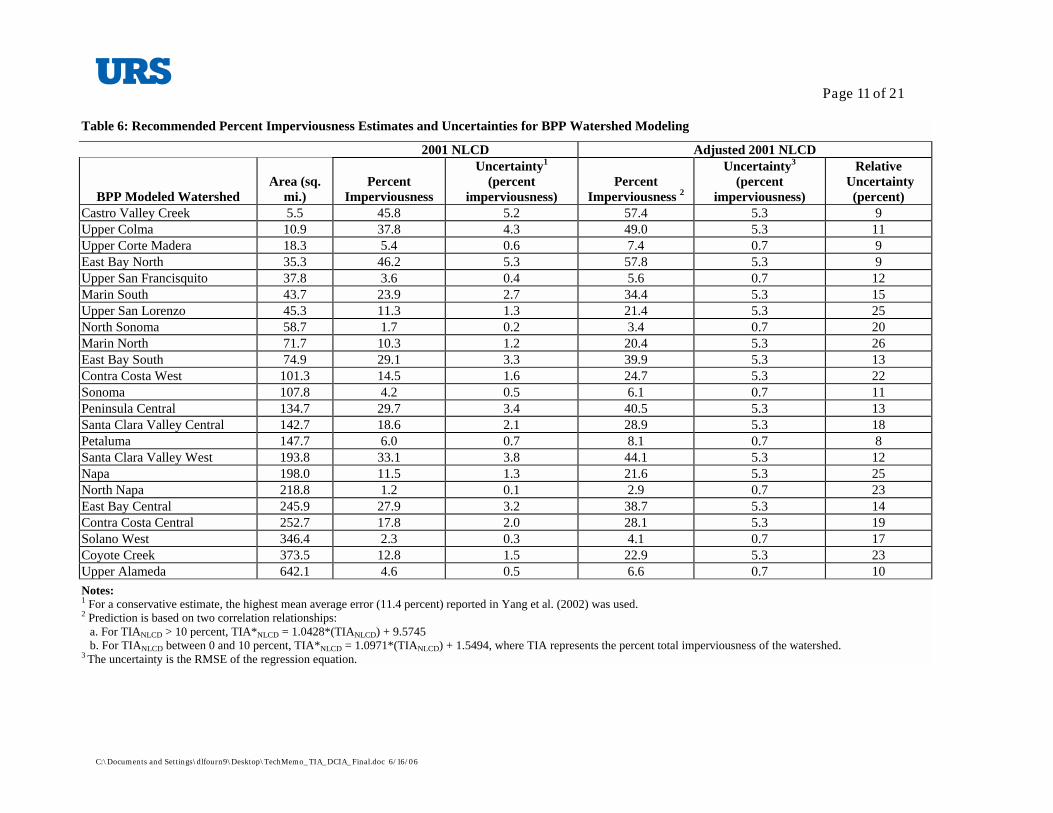
The uncertainties associated with the adjusted NLCD estimates are the unexplained error of the regressions, which is quantified by the RMSE. The unexplained error is 0.7 percentage point for imperviousness between 0 and 10 percent (Figure 2a) and 5.3 percentage point for imperviousness greater than 10 percent (Figure 3a). Among the BPP-modeled watersheds, imperviousness ranges between 3.4 percent in the North Sonoma watershed to 57.8 percent in the East Bay North watershed. Relative uncertainties vary between 8 percent in the Petaluma watershed and 26 percent in the Marin North watershed. The mean, median, and standard deviation of the relative uncertainties are 16, 14, and 6 percent, respectively.

Page 11 of 21

C:\Documents and Settings\dlfourn9\Desktop\TechMemo_TIA_DCIA_Final.doc 6/16/06

Table 6: Recommended Percent Imperviousness Estimates and Uncertainties for BPP Watershed Modeling

2001 NLCD Adjusted 2001 NLCD

BPP Modeled Watershed Area (sq.

mi.) Percent

Imperviousness

Uncertainty1 (percent

imperviousness) Percent

Imperviousness 2

Uncertainty3 (percent

imperviousness)

Relative Uncertainty

(percent) Castro Valley Creek 5.5 45.8 5.2 57.4 5.3 9 Upper Colma 10.9 37.8 4.3 49.0 5.3 11 Upper Corte Madera 18.3 5.4 0.6 7.4 0.7 9 East Bay North 35.3 46.2 5.3 57.8 5.3 9 Upper San Francisquito 37.8 3.6 0.4 5.6 0.7 12 Marin South 43.7 23.9 2.7 34.4 5.3 15 Upper San Lorenzo 45.3 11.3 1.3 21.4 5.3 25 North Sonoma 58.7 1.7 0.2 3.4 0.7 20 Marin North 71.7 10.3 1.2 20.4 5.3 26 East Bay South 74.9 29.1 3.3 39.9 5.3 13 Contra Costa West 101.3 14.5 1.6 24.7 5.3 22 Sonoma 107.8 4.2 0.5 6.1 0.7 11 Peninsula Central 134.7 29.7 3.4 40.5 5.3 13 Santa Clara Valley Central 142.7 18.6 2.1 28.9 5.3 18 Petaluma 147.7 6.0 0.7 8.1 0.7 8 Santa Clara Valley West 193.8 33.1 3.8 44.1 5.3 12 Napa 198.0 11.5 1.3 21.6 5.3 25 North Napa 218.8 1.2 0.1 2.9 0.7 23 East Bay Central 245.9 27.9 3.2 38.7 5.3 14 Contra Costa Central 252.7 17.8 2.0 28.1 5.3 19 Solano West 346.4 2.3 0.3 4.1 0.7 17 Coyote Creek 373.5 12.8 1.5 22.9 5.3 23 Upper Alameda 642.1 4.6 0.5 6.6 0.7 10 Notes: 1 For a conservative estimate, the highest mean average error (11.4 percent) reported in Yang et al. (2002) was used. 2 Prediction is based on two correlation relationships:

a. For TIANLCD > 10 percent, TIA*NLCD = 1.0428*(TIANLCD) + 9.5745 b. For TIANLCD between 0 and 10 percent, TIA*NLCD = 1.0971*(TIANLCD) + 1.5494, where TIA represents the percent total imperviousness of the watershed.

3 The uncertainty is the RMSE of the regression equation.

Page 12 of 21

C:\Documents and Settings\dlfourn9\Desktop\TechMemo_TIA_DCIA_Final.doc 6/16/06

3.0 ESTIMATION OF DIRECTLY CONNECTED IMPERVIOUS AREAS DCIA, also referred to as effective impervious area, is an important parameter for stormwater runoff modeling in urban watersheds because it directly affects the volume and quality of runoff discharged to receiving waters (Schueler 1994). DCIA is the portion of the TIA generating stormwater runoff that discharges directly into a stormwater collection system or a receiving water body without flowing over any pervious surfaces. Direct measurement of DCIA is an expensive and time-consuming process, involving extensive field observations to evaluate and catalog the hydraulic connection between impervious areas and the stormwater collection system. Few accurate measurements of DCIA have been performed. Methods for estimating DCIA typically rely on land use and land cover data, and GIS analysis. In support of the BPP’s watershed modeling effort, URS (1) conducted a literature review to identify available methods for estimating DCIA, (2) identified the methods most appropriate for the BPP’s purposes, (3) applied these methods to the BPP-modeled watersheds using the corrected NLCD data on TIA, (4) performed a reality check on the resultant DCIA estimates using road surface area and inverse parcel area estimates, and (5) recommended a method to the BPP for estimating DCIA.

3.1 LITERATURE REVIEW Estimating DCIA is a complicated task since many factors affect the extent to which impervious areas are directly connected to stormwater systems and receiving waters, including, for example, land use and building practices at the time an area was developed. Through the literature review, URS identified three basic approaches to estimating DCIA: (1) developing coefficients for each land use, (2) comparing rainfall and runoff volumes, and (3) deriving empirical relationships between DCIA and TIA. Methods Using Land Use Coefficients A study of DCIA in the Rouge River Watershed in Michigan developed coefficients by land use based on digital land use data and aerial photographs (RPO 1994). The land use data consist of polygons coded by land use. Percent imperviousness was estimated using a 1”=200’ enlargement of aerial photographs for two sample areas within each subwatershed. In each subwatershed sample area, three small sample areas were selected for each of the 10 land use categories; a total of 300 sample areas were examined on aerial photographs and in the field. Pervious and impervious areas in the aerial photographs were measured for features such as buildings, roads, parking areas, driveways, sidewalks, bikepaths, and water bodies, including swimming pools. Paved, dirt, and gravel roads, parking areas, and driveways were all considered impervious. The percent DCIA of a given land use category within a subwatershed was estimated based on field evaluation of the sample areas. Using the collected data, average percent impervious area and average percent DCIA for each land use category within a subwatershed was calculated. Statistics of DCIA percentages per land use found in subwatersheds are presented in Table 7.

Table 7. Statistics of DCIA Estimates Per Land Use for the Rouge River Watershed in Michigan (RPO 1994)

DCIA (percent)

Land Use Average Standard Deviation Min Max

Forest/Rural Open 3.8 5.0 0.0 16.1 Urban Open 8.1 5.7 0.0 18.9 Agricultural/Pasture 2.1 2.0 0.0 5.3 Low Density Residential 11.5 10.7 0.0 30.2 Medium Density Residential 27.7 15.6 0.0 52.3 High Density Residential 39.7 19.0 0.0 67.4 Commercial 47.1 15.9 11.3 66.8 Industrial 67.6 27.9 2.2 92.0 Highway 37.0 30.6 0.0 90.9 Water/Wetlands 46.2 27.1 0.0 100.0

Page 13 of 21

C:\Documents and Settings\dlfourn9\Desktop\TechMemo_TIA_DCIA_Final.doc 6/16/06

The imperviousness of transportation-related land uses in urban areas is often assumed to be 100 percent directly connected to stormwater collection system. Buchan (1999) suggested that a good estimate of DCIA can be calculated using high-accuracy road area data. The City of Olympia, Washington (1994) conducted an extensive analysis of 11 residential and commercial sites to understand imperviousness contribution per land use and found that approximately 63 to 70 percent of TIA is related to transportation, including roads, driveways, and parking lots. DCIA estimates based on road data can be improved by combining them with lower-accuracy land use data. In a study of a residential area in Boulder, Colorado (Lee and Heaney 2003), in which paved streets with curbs were considered DCIA and streets without curbs were not, researchers found that 64 percent of the TIA is comprised of transportation-related impervious surfaces, including streets, sidewalks, and driveways. A more detailed analysis using GIS and field investigation, found that 68.9 percent of streets, 28.3 percent of driveways, 68.2 percent of sidewalks, and only 2.9 percent of building rooftops were DCIA, representing 13 percent of the entire study area and 36 percent of the TIA. They also found that transportation-related DCIA represents 97.2 percent of total DCIA. The street pavement is the largest portion of DCIA with 68 percent of the whole DCIA. They concluded that condition of the street boundary (i.e., with or without curb) can be an important determinant of urban DCIA. Based on these findings, DCIA in urban areas could be fairly well estimated using road right-of-way area including sidewalks and shoulders. This area can be derived from parcel data assuming that it is well represented by the “inverse parcel” area. The “inverse” parcel area is the area not defined as a parcel. Using detailed GIS datasets, Hoffman and Crawford (2001) developed impervious cover maps for single-family residential and commercial areas of Portland, Oregon. They estimated that 86 percent of single-family residential impervious areas and 100 percent of other impervious areas (i.e., streets, commercial buildings, and parking lots) are directly connected surfaces. Lee and Heaney (2003) estimated the DCIA for a high-density residential area of Miami was 44.1 percent, assuming that parking lots and paved streets were DCIA and building rooftops and other miscellaneous impervious surfaces were not. Methods Using Rainfall and Runoff Measurements Another approach to estimating DCIA is to look at detailed rainfall-runoff data to predict runoff from pervious and impervious surfaces. Boyd et al. (1993, 1994) assumed that for small storms only impervious surfaces would contribute to runoff, but that for large storms, both pervious and impervious surfaces would contribute to runoff. DCIA was estimated by plotting rainfall depth versus runoff depth. This type of analysis requires detailed rainfall-runoff data. Sutherland (1995) reports using a rainfall-runoff model, for which DCIA is a parameter, in a gauged watershed. By fixing reasonable estimates of other model parameters, he was able to calibrate the model by varying DCIA to meet runoff peaks and volumes. He recommends repeating the calibration for several storm events, and averaging storm DCIA values to obtain a final DCIA estimate. This method could be extended to continuous simulation modeling instead of event modeling, suggesting that some tuning to DCIA parameters should be done during BPP watershed modeling calibration. Methods Using Empirical Relationships Alley and Veenhuis (1983) developed the following equation for the highly urban portion of Denver, Colorado. The relationship was developed through mapping of street surface areas and field inspection of other impervious areas in 14 drainage basins to determine if they were directly connected. Note that this empirically derived estimate is not a function of land-use and is therefore not necessarily valid for other locations where mixes of land-use and building codes may differ from the Denver basins due to develop the relationship.

41.115.0 TIADCIA = The R-square coefficient was 0.98 and the standard error of estimate was 7.5%. The USGS (Laenen 1983) developed the following equation for watersheds in the metropolitan areas of Portland and Salem, Oregon. This relationship was developed using a combination of field verification of directly connected impervious areas, and detailed rainfall-runoff modeling (using 5-minute rainfall and stream gage data) for four basins within the Willamette Valley. It should be noted that the authors did not find a good fit using the above empirical equation for some basins in Portland and Vancouver, Oregon, due to differing soil types, and unpredictable use of dry wells for roof drain connections.

TIADCIA 43.06.3 +=

Page 14 of 21

C:\Documents and Settings\dlfourn9\Desktop\TechMemo_TIA_DCIA_Final.doc 6/16/06

Laenen found that the coefficient R-square for the linear regression equation was of 0.84 and the standard error of estimate 27 percent. The author cites volcanic rock outcrops as an explanation of the non-zero intercept for the Willamette Valley. Based on the USGS modeling, mapping of imperviousness, and field observations described above (Laenen 1983), Sutherland (1995) developed five equations for estimating DCIA for watersheds having different conditions:

%1)(1.0 5.1

≥=

TIATIADCIA

Average basins: “Local drainage collector systems for the urban areas are predominantly storm sewered with curb and gutters stormwater, no infiltration areas and rooftops in the single-family residential areas are disconnected.”

%1)(4.0 2.1

≥=

TIATIADCIA

Highly connected basins: Same conditions as for Average basins with residential rooftops directly connected to stormwater collection systems.

TIADCIA = Totally connected basins: All urban areas are directly connected to stormwater collection systems.

%1)(04.0 7.1

≥=

TIATIADCIA

Somewhat disconnected: Approximately 50 percent of urban areas are disconnected form stormwater collection systems.

%1)(01.0 6.2

≥=

TIATIADCIA

Extremely disconnected: Small percentage of urban areas are directly connected or 70 percent or more of basin area drains to dry wells and other infiltration areas.

Sutherland recommends on-site investigation of the basins to select the appropriate DCIA equation. The strength of these equations according to Sutherland is their consistency in providing reasonable estimates of DCIA over the entire range of TIA. Discussion The BPP has already determined that the USGS 2001 NLCD data, which includes a percentage impervious data layer, is the best available land use and land cover data for use in the BPP’s watershed modeling effort (Sustainable Conservation 2005). Given the nature of this data, it is most appropriate for the BPP to use one of the estimation methods based on empirical relationships to estimate DCIA. The following provides a comparison and assessment of the DCIA estimates produced using these three methods.

3.2 METHOD Using the three empirical methods identified through the literature review—Alley and Veenhuis (1983), Laenen (1983), and Sutherland (1995)—URS calculated DCIA and the associated uncertainty from the adjusted 2001 NLCD TIA estimates for each of the 23 BPP-modeled watersheds. As a “reality check,” URS compared the results with inverse parcel data and road surface area estimates (URS, 2006). Alley and Veenhuis (1983) and Laenen (1983) each provide a single equation for estimating DCIA. Sutherland (1995) developed five equations corresponding to different basin conditions. URS determined that Sutherland’s “average conditions” were the most analogous to those in the San Francisco Bay area, and used that equation. URS calculated uncertainties in DCIA estimates based on those for the TIA estimates. This approach does not consider the regression error generated with the empirical equations or the uncertainty associated with the application of equations developed for other parts of the country having different land use patterns, development histories, and building codes. The DCIA results from the Rouge River Program (Table 7) show great variability in DCIA per land use and, therefore, a significant uncertainty associated with the regression equation. Unfortunately, the uncertainties associated with the application of the methods in another region cannot be derived easily or reliably and, thus, are not included in the uncertainty estimates calculated here.

Page 15 of 21

C:\Documents and Settings\dlfourn9\Desktop\TechMemo_TIA_DCIA_Final.doc 6/16/06

TIA uncertainties were propagated using the propagation of error equation, the first term in the Taylor series approximation for the propagation of uncertainty, which can be used when variables are not correlated. Uncertainties were calculated according to the following equation:

( )

( )

. equations empiricalfor y uncertaint theis

6, Table from estimateTIA NLCD adjustedon y uncertaint theis

of derivativefirst theis

equations, empiricalDCIA three theof equation represents )(Where

3

1

2

i

fdTIA

TIAdfiTIAf

dTIATIAdf

i

i

i

DCIA

TIA

ii

i

i

iTIAiDCIA

σ

σ

σσ ∑=

×=

For comparison purposes, the resulting DCIA estimates were plotted with road surface area and available inverse parcel area. Road surface area was calculated for all 23 BPP-modeled watersheds developed from local data (URS 2006) (Table 8) and ESRI’s U.S. Streets layer (ESRI 2004).

Table 8. URS Road Width Estimates for ESRI Road Categories

BPP-Modeled Watershed

BPP-Modeled WatershedArea

(sq mi)

Road Surface Area

(sq mi)

Road Surface Area

Uncertainty(sq mi)

Castro Valley Creek 5.5 0.7 0.2 8.9 - 14.8Upper Colma 10.9 1.3 0.2 9.8 - 14.3Upper Corte Madera 18.3 1.1 0.2 4.4 - 7.2East Bay North 35.3 5.5 1.1 12.3 - 18.8Upper San Francisquito 37.8 1.0 0.2 2.1 - 3.3Marin South 43.7 3.2 0.7 5.8 - 8.8Upper San Lorenzo 45.3 1.8 0.4 3.1 - 4.7North Sonoma 58.7 1.5 0.3 1.9 - 3.1Marin North 71.7 3.2 0.7 3.5 - 5.4East Bay South 74.9 4.4 1.0 4.6 - 7.2Contra Costa West 101.3 4.9 1.1 3.8 - 5.9Sonoma 107.8 2.6 0.6 1.9 - 3.0Peninsula Central 134.7 12.5 2.3 7.5 - 11.0Santa Clara Valley Central 142.7 17.5 3.7 9.7 - 14.9Petaluma 147.7 4.4 0.9 2.4 - 3.6Santa Clara Valley West 193.8 17.5 3.7 7.1 - 10.9Napa 198 7.3 1.4 3.0 - 4.4North Napa 218.8 3.3 0.5 1.3 - 1.8East Bay Central 245.9 19.0 4.2 6.0 - 9.4Contra Costa Central 252.7 15.3 3.3 4.8 - 7.3Solano West 346.4 7.2 1.4 1.7 - 2.5Coyote Creek 373.5 12.6 2.7 2.7 - 4.1Upper Alameda 642.1 13.0 2.9 1.6 - 2.5

Percentage of Watershed Area

Covered by Roads (%)

Inverse parcel area is the area that is not a part of a real estate parcel. It includes public roads, sidewalks, and rights-of-way, and does not include residential driveways, rooftops, or commercial buildings and parking lots. URS collected parcel data

Page 16 of 21

C:\Documents and Settings\dlfourn9\Desktop\TechMemo_TIA_DCIA_Final.doc 6/16/06

for Contra Costa and Sonoma counties and analyzed it using ArcGIS to derive inverse parcel area. Inverse parcel area data for Santa Clara County were provided by EOA, Inc. Inverse parcel areas were calculated for the seven BPP-modeled watersheds that are fully enclosed in Santa Clara, Sonoma, and Contra Costa counties.

3.3 RESULTS DCIA estimates are presented in Table 9 and on Figure 4 along with road surface areas and inverse parcel areas. For those watersheds having DCIA estimates of less than 5 percent, the estimated DCIA with Alley and Veenhuis (1983) and Sutherland (1995) matched closely with the total road surface area and inverse parcel area estimates. The closeness of the estimates with the road surface area and inverse parcel area estimates matches well with the understanding that in watersheds having low imperviousness, road area represents almost all of the DCIA. Watersheds having DCIA estimates of less than 1 percent include North Napa, North Sonoma, Solano West and Upper Alameda. Estimates obtained using Laenen (1983) equation produced estimates consistently higher than the two other equations (i.e. about 4 percentage points) and do not seem to be realistic estimates. The three equations produce similar estimates for watersheds having between 10 and 20 percent DCIA. For these watersheds, road surface area accounts for approximately 30 to 40 percent of the DCIA, and inverse parcel area accounts for 40 to 50 percent of the total estimated DCIA. Eight watersheds (of 23) have DCIA values between 10 and 20 percent. For DCIA values greater than 20 percent, the Alley and Veenhuis (1983) and Sutherland (1995) equations generate similar estimates, while the Laenen (1983) equation produces lower values. Road area accounts for 20 to 35 percent of total DCIA using Alley and Veenhuis (1983) and Sutherland (1995) equations. Road area accounts for a greater proportion (between 30 to 55 percent) of DCIA using Laenen (1983). Watersheds having DCIA estimates of greater than 30 percent include Santa Clara Valley West, Castro Valley Creek, Upper Colma, and East Bay North. For watersheds having estimated DCIA values greater than 10 percent, a general trend of all three estimation methods indicates that road surface area accounts for a smaller percentage of the total estimated DCIA, reflecting that more heavily developed areas tend to have greater amounts of nonroad DCIA (e.g., buildings, parking lots, and other paved surfaces). For the watersheds having estimated DCIA values greater than 15 percent, the Alley and Veenhuis (1983) and Sutherland (1995) estimation methods indicate that road surface area accounts for as little as 22 percent (i.e. East Bay South) of the estimated DCIA to as much as 79 percent (i.e. Santa Clara Valley Central). Without the value from Santa Clara Valley Central, road area contribution to DCIA is centered around 33 percent with a 6 percent standard deviation. The Laenen (1983) estimation method, which produces lower estimates of DCIA for these watersheds, shows that road surface area may account for as little as 25 percent of the estimated DCIA and as much as 76 percent (i.e. Santa Clara Valley Central). For Laenen (1983) relationship, road area contribution averages 39 percent with a standard deviation of 8 percent without Santa Clara Valley Central. Uncertainties for estimates obtained with Alley and Veenhuis (1983) and Laenen (1983) relationships are generally greater than for Sutherland (1995) estimates because they account for the uncertainty in the method. The method uncertainty was not available for Sutherland (1995) relationship. DCIA values obtained with Alley and Veenhuis (1983) and Laenen (1983) relationships have uncertainties between 14 and 38 percent with an average and standard deviation of 26 percent and 6 percent, respectively.

Page 17 of 21

C:\Documents and Settings\dlfourn9\Desktop\TechMemo_TIA_DCIA_Final.doc 6/16/06

Table 9: Calculation of DCIA Estimates and Uncertainties Using Three Empirical Equations and Comparison With Road Surface Area and Inverse Parcel Area for BPP-Modeled Watersheds

Adjusted NLCD Alley & Veenhuis (1983) Laenen (1983) Sutherland (1995)

BPP-Modeled Watershed

Area (sq. mi.)

TIA (percent of watershed)

TIA Relative

Uncertainty(percent

TIA)

DCIA = 0.15(TIA)1.41

(percent of watershed)

DCIA Relative

Uncertainty(percent DCIA)

DCIA = 3.6 + 0.43(TIA)(percent of watershed)

DCIA Relative

Uncertainty (percent DCIA)

Average Basin

DCIA = 0.1(TIA)1.5

TIA > 1 %(percent of watershed)

DCIA Relative

Uncertainty(percent DCIA)

Road Surface

Area (percent of watershed)

Inverse Parcel Area(percent of watershed)

Castro Valley Creek 5.5 57.4 9 45.3 15 28.3 28 43.5 14 2.9 Upper Colma 10.9 49.0 11 36.3 17 24.7 29 34.3 16 2.2 Upper Corte Madera 18.3 7.4 9 2.5 15 6.8 27 2.0 14 1.4 East Bay North 35.3 57.8 9 45.7 15 28.4 28 43.9 14 3.2 Upper San Francisquito 37.8 5.6 12 1.7 19 6.0 27 1.3 18 0.6 Marin South 43.7 34.4 15 22.1 23 18.4 30 20.2 23 1.5 Upper San Lorenzo 45.3 21.4 25 11.3 36 12.8 32 9.9 37 0.8 North Sonoma 58.7 3.4 20 0.9 29 5.1 28 0.6 30 0.6 1.4 Marin North 71.7 20.4 26 10.5 38 12.4 33 9.2 39 0.9 East Bay South 74.9 39.9 13 27.1 20 20.7 29 25.2 20 1.3 Contra Costa West 101.3 24.7 22 13.8 31 14.2 31 12.2 32 1.1 7.5 Sonoma 107.8 6.1 11 1.9 17 6.2 27 1.5 17 0.5 3.8 Peninsula Central 134.7 40.5 13 27.8 20 21.0 29 25.8 20 1.7 Santa Clara Valley Central 142.7 28.9 18 17.2 27 16.0 31 15.6 28 2.6 8.7

Petaluma 147.7 8.1 8 2.9 14 7.1 27 2.3 13 0.6 Santa Clara Valley West 193.8 44.1 12 31.2 19 22.5 29 29.2 18 1.9 12.8 Napa 198.0 21.6 25 11.4 36 12.9 32 10.0 37 0.7 North Napa 218.8 2.9 23 0.7 34 4.9 28 0.5 35 0.2 East Bay Central 245.9 38.7 14 25.9 21 20.2 29 24.0 21 1.7 Contra Costa Central 252.7 28.1 19 16.5 28 15.7 31 14.9 28 1.3 8.2 Solano West 346.4 4.1 17 1.1 24 5.4 28 0.8 25 0.4 Coyote Creek 373.5 22.9 23 12.4 34 13.5 32 11.0 35 0.7 4.8 Upper Alameda 642.1 6.6 10 2.2 16 6.4 27 1.7 15 0.4

Page 18 of 21

C:\Documents and Settings\dlfourn9\Desktop\TechMemo_TIA_DCIA_Final.doc 6/16/06

Figure 4: Comparison of Three DCIA Estimates with Road Surface Areas and Inverse Parcel Areas for the BPP-Modeled Watersheds

0

5

10

15

20

25

30

35

40

45

50

55

60

North N

apa

North S

onom

aSola

no W

est

Upper

San Fran

cisqu

itoSon

oma

Upper

Alamed

a

Upper

Corte M

adera

Petalum

aMari

n Nort

h

Upper

San Lo

renzo

Napa

Coyote

Cree

k

Contra

Cos

ta W

est

Contra

Cos

ta Cen

tral

Santa

Clara V

alley

Cen

tral

Marin S

outh

East B

ay C

entra

lEas

t Bay

Sou

th

Penins

ula C

entra

l

Santa

Clara V

alley

Wes

tUpp

er Colm

a

Castro

Vall

ey C

reek

East B

ay N

orth

BPP Modeled Watershed

Perc

enta

ge o

f Wat

ersh

ed

Alley and Veenhuis, 1983 Laenen, 1983 Sutherland, 1995 Road Surface Area Inverse Parcel Area

Page 19 of 21

C:\Documents and Settings\dlfourn9\Desktop\TechMemo_TIA_DCIA_Final.doc 6/16/06

3.4 CONCLUSIONS Empirical equations from Alley and Veenhuis (1983) and Sutherland (1995) produce similar DCIA estimates. For DCIA less than 5 percent, estimates match road surface areas. All three equations generate similar estimates between 10 and 15 percent DCIA. For DCIA greater than 10 percent, Alley and Veenhuis (1983) and Sutherland (1995) estimates are much greater than road areas, which then represent between 21 and 58 percent of the total DCIA. By comparison, Lee and Heaney (2003) found that road surface area accounted for 68 percent of the total DCIA in a residential area of Boulder, Colorado. The average uncertainty is approximately 26 percent with a standard deviation of 6 percent. It was broadly assumed that these equations could be extrapolated to the San Francisco Bay area.

3.5 RECOMMENDATIONS URS recommends using the empirical equation from Alley and Veenhuis (1983) to estimate DCIA for BPP-modeled watersheds, and propagate through the uncertainty estimates associated with the TIA estimates. Although empirical estimation methods have inherent weaknesses as discussed above in the literature review section, and no empirical estimation method is available specifically for the San Francisco Bay area, this type of approach is most appropriate to the data the BPP has decided to use (Sustainable Conservation 2005). In addition, the reality checks conducted here indicate that the methods have generated DCIA estimates within a reasonable range and with enough accuracy for an initial value in the calibration of BPP watershed model. The Alley and Veenhuis (1983) and Sutherland (1995) methods produce similar results for the full range of TIA with which the BPP is working. The Laenen (1983) method generates high DCIA values for watersheds having less than 10 percent TIA and, thus, is not recommended for use by the BPP. In choosing between the Alley and Veenhuis (1983) and Sutherland (1995) approaches, URS recommends using the Alley and Veenhuis (1983) approach because it has been published in a peer-reviewed scientific journal.

Table 10: Recommended DCIA Estimates and Uncertainties for BPP-Modeled Watersheds

Adjusted NLCD Alley and Veenhuis (1983)

BPP-Modeled Watershed Area

(sq. mi.)

TIA (percent of watershed)

TIA Relative Uncertainty

(percent)

DCIA = 0.15(TIA)1.41

(percent of watershed)

DCIA Relative Uncertainty

(percent)

Road Surface Area(percent of watershed)

Road Surface Area

(percent of DCIA)

Castro Valley Creek 5.5 57.4 9 45.3 15 2.9 26 Upper Colma 10.9 49.0 11 36.3 17 2.2 33 Upper Corte Madera 18.3 7.4 9 2.5 15 1.4 228 East Bay North 35.3 57.8 9 45.7 15 3.2 34 Upper San Francisquito 37.8 5.6 12 1.7 19 0.6 162 Marin South 43.7 34.4 15 22.1 23 1.5 33 Upper San Lorenzo 45.3 21.4 25 11.3 36 0.8 35 North Sonoma 58.7 3.4 20 0.9 29 0.6 291 Marin North 71.7 20.4 26 10.5 38 0.9 43 East Bay South 74.9 39.9 13 27.1 20 1.3 22 Contra Costa West 101.3 24.7 22 13.8 31 1.1 35 Sonoma 107.8 6.1 11 1.9 17 0.5 126 Peninsula Central 134.7 40.5 13 27.8 20 1.7 33 Santa Clara Valley Central 142.7 28.9 18 17.2 27 2.6 71 Petaluma 147.7 8.1 8 2.9 14 0.6 103 Santa Clara Valley West 193.8 44.1 12 31.2 19 1.9 29 Napa 198.0 21.6 25 11.4 36 0.7 32 North Napa 218.8 2.9 23 0.7 34 0.2 224 East Bay Central 245.9 38.7 14 25.9 21 1.7 30 Contra Costa Central 252.7 28.1 19 16.5 28 1.3 37 Solano West 346.4 4.1 17 1.1 24 0.4 189 Coyote Creek 373.5 22.9 23 12.4 34 0.7 27 Upper Alameda 642.1 6.6 10 2.2 16 0.4 94

Page 20 of 21

C:\Documents and Settings\dlfourn9\Desktop\TechMemo_TIA_DCIA_Final.doc 6/16/06

REFERENCES Alameda County Public Works Agency (ACPWA). 1998. Land use classification of Castro Valley,

cvlanduse.shp. Water Resources Division.

Alley, W.M., and J.E. Veenhuis. 1983. Effective impervious area in urban runoff modeling. J.Hydraul.Eng. 109(2): 313-319.

Association of Bay Area Governments (ABAG). 1996. Existing Land Use in 1995: Data for Bay Association of Bay Governments, Area Counties, and Cities. Publication Number P96007EQK.

Bredehorst, E. 1981. Benefit Assessment Runoff Factor Study. Unpublished study for the Los Angeles Flood Control District, Los Angeles, CA.

Boyd, M.J., M.C. Bulfill, and R.M. Knee. 1993. Pervious and impervious runoff in urban catchments. Hydrol. Sci. J. 38(6): 463-478.

Boyd, M.J., M.C. Bulfill, and R.M. Knee. 1994. Predicting pervious and impervious storm runoff from urban drainage basins. Hydrol. Sci. J. 39(4): 321-332.

Buchan, L. 1999. Technical Memorandum: Indicator #24, Growth and Development (Imperviousness). Interim Work Product. Santa Clara Valley Urban Runoff Pollution Prevention Program.

Carleton, J.N. 2004. Watershed modeling for the environmental fate and transport of copper from vehicle brake pad wear debris work plan. Accessed online at http://www.suscon.org/brakepad/pdfs/FinalWatershedModelingWorkPlanCarleton(11-19-04).pdf

City of Olympia. 1994. Impervious Surface Reduction Study. Draft Final Report. Public Works Department, Olympia, WA.

EOA Inc. 1997. Pilot Study Evaluating Watershed Management Tools for the Lower San Mateo Creek Watershed. Prepared for the San Mateo Countywide Stormwater Pollution Prevention Program. Oakland, CA.

EOA Inc. 1998. Imperviousness as a Watershed Management Tool for San Mateo County Watersheds. Prepared for the San Mateo Countywide Stormwater Pollution Prevention Program. Oakland, CA.

EOA Inc. 1999. Imperviousness Estimates for Five Watersheds in San Mateo County. Prepared for the San Mateo Countywide Stormwater Pollution Prevention Program. Oakland, CA.

EOA Inc. 2000a. Chapter 4 Land Use in Unabridged Watershed Characteristics Report. Prepared for Santa Clara Valley Urban Runoff Pollution Prevention Program (SCVURPPP).

EOA Inc., 2000b. Characterization of Imperviousness and Creek Channel Modifications for Six Watersheds in San Mateo County. Prepared for the San Mateo Countywide Stormwater Pollution Prevention Program. Oakland, CA.

ESRI. 2004. ESRI® Data & Maps 2004 - An ESRI White Paper. Accessed online at http://www.esri.com/library/whitepapers/pdfs/datamaps2004.pdf.

Hoffman, J., and D. Crawford. 2001. Using comprehensive mapping and database management to improve urban sewer systems. In Models and Applications to Urban Water Systems. W. James, ed., pp. 445-464.CHI Publications, Guelph, Ont., Canada.

Khan, O., Shawley, G., Chen, C.L., and Chen, C.W. 1996. Castro Valley Water Quality Modeling, Calibration and Verification. ACFCWCD.

Page 21 of 21

C:\Documents and Settings\dlfourn9\Desktop\TechMemo_TIA_DCIA_Final.doc 6/16/06

Laenen, A. 1983. Storm runoff as related to urbanization based on data collected in Salem and Portland and generalized for the Willamette Valley, Oregon. USGS Water Resources Investigations Open File Report 83-4143.

Lee, J.G., and J.P. Heaney. 2003. Estimation of urban imperviousness and its impacts on storm water systems. Journal of Water Resources Planning and Management 129 (5): 419-426. ASCE.

Multi-Resolution Land Characteristics Consortium (MRLC). 2001. National Land Cover Database 2001 (NLCD 2001). Accessed online at http://www.mrlc.gov/mrlc2k_nlcd.asp.

San Mateo Countywide Stormwater Pollution Prevention Program (STOPPP). 2002. Characterization of imperviousness and creek channel modifications for seventeen watersheds in San Mateo County.

Schueler, T.R., 1994. The importance of imperviousness. Watershed Protection Techniques 1(3): 100-111.

Sustainable Conservation. 2005. Memorandum: The use of land cover and land use data as data inputs and its impact on BPP technical studies. Written by Sarah Connick & Connie Liao. February 1. Accessed online at http://www.suscon.org/brakepad/pdfs/LandUseDataforModelsandEstimatesMemoFinal(02-01-06).pdf

Sutherland, R. 1995. Methodology for estimating the effective impervious area of urban watersheds. Technical Notes 58, Watershed Protection Techniques2 (1). Center for Watershed Protection

URS Corporation. 2006. BPP Land Use and Land Cover Analysis for Air Modeling. Memorandum to Sarah Connick, Sustainable Conservation, from Alexis Dufour, Fan Lau, and Terry Cooke, April 2006

Wayne County Rouge Program Office (RPO). 1994. Determination of Impervious Area and Directly Connected Impervious Area.

Yang, L, C. Huang, C. Homer, B. Wylie, and M. Coan. 2002. An approach for mapping large-area impervious surfaces: Synergistic use of Landsat 7 ETM+ and high spatial resolution imagery. Canadian Journal of Remote Sensing 29 (2): 230-240. Accessed online at http://landcover.usgs.gov/pdf/imppaperfinalwithall.pdf.