Databases 2 Storage optimization: functional dependencies, normal forms, data ware houses.
110
Databases 2 Storage optimization: functional dependencies, normal forms, data ware houses
-
Upload
shawn-black -
Category
Documents
-
view
241 -
download
4
Transcript of Databases 2 Storage optimization: functional dependencies, normal forms, data ware houses.
Databases 2
Storage optimization: functional dependencies, normal forms, data
ware houses
Functional Dependencies
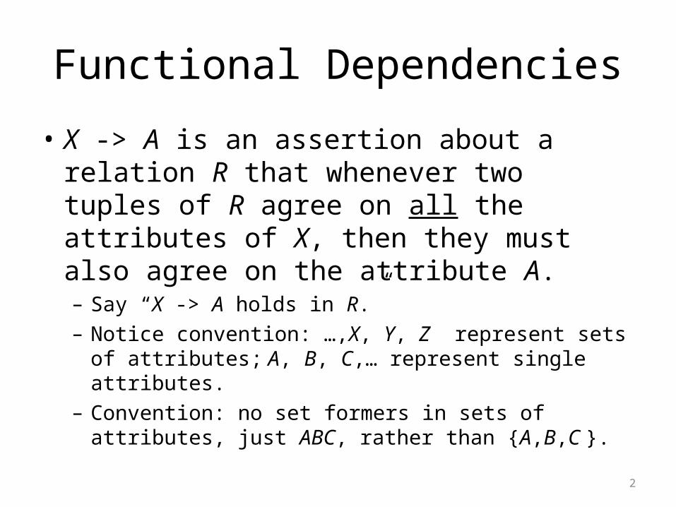
• X -> A is an assertion about a relation R that whenever two tuples of R agree on all the attributes of X, then they must also agree on the attribute A.– Say “X -> A holds in R.”– Notice convention: …,X, Y, Z represent sets of attributes;
A, B, C,… represent single attributes.– Convention: no set formers in sets of attributes, just ABC,
rather than {A,B,C }.
2
Example
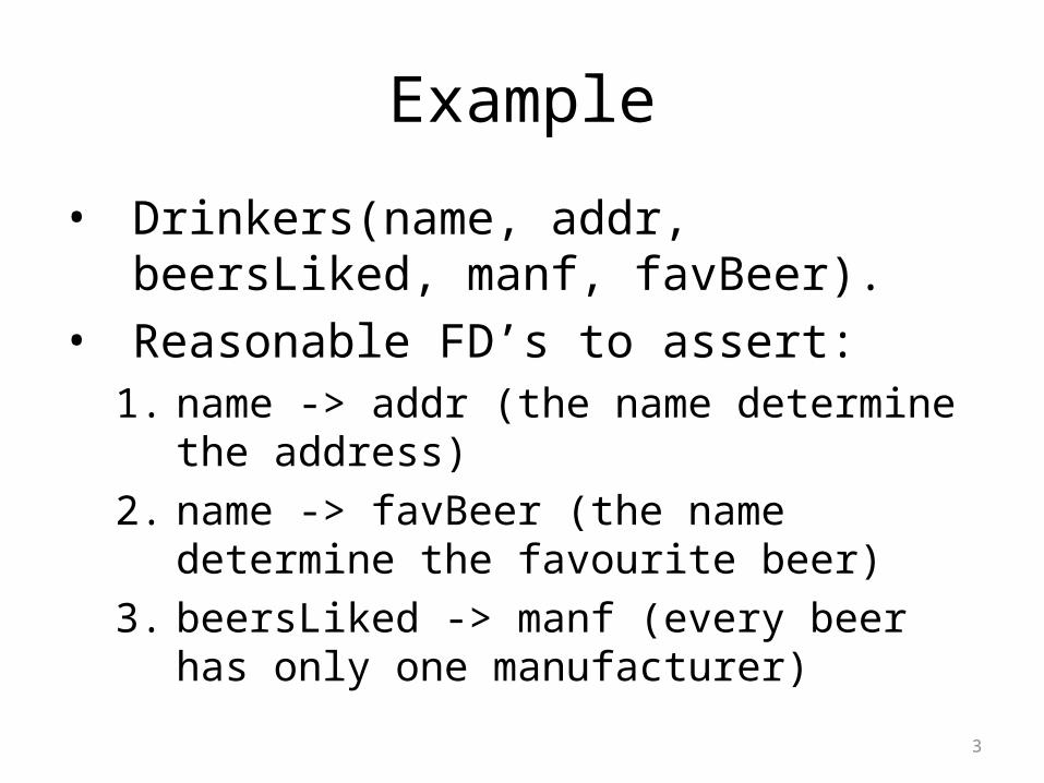
• Drinkers(name, addr, beersLiked, manf, favBeer).
• Reasonable FD’s to assert:1. name -> addr (the name determine the address)2. name -> favBeer (the name determine the
favourite beer)3. beersLiked -> manf (every beer has only one
manufacturer)
3
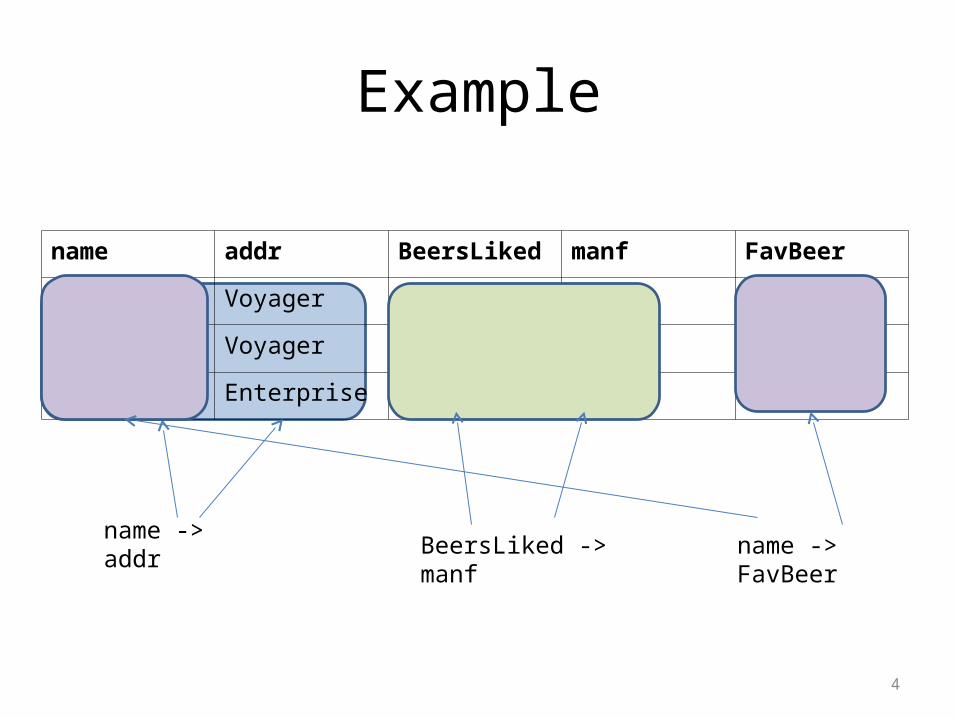
Example
4
name addr BeersLiked manf FavBeer
Janeway Voyager Bud A.B. WickedAle
Janeway Voyager WickedAle Pete’s WickedAle
Spock Enterprise Bud A.B. Bud
name -> addrname -> FavBeerBeersLiked -> manf

FD’s With Multiple Attributes
• No need for FD’s with more than one attribute on right.– But sometimes convenient to combine FD’s as a
shorthand.– Example: name -> addr and name -> favBeer
become name -> addr favBeer• More than one attribute on left may be
essential.– Example: bar beer -> price
5
Keys of Relations
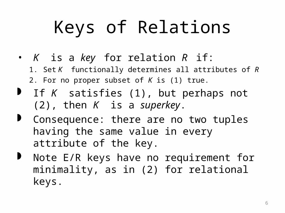
• K is a key for relation R if:1. Set K functionally determines all attributes of R2. For no proper subset of K is (1) true.
If K satisfies (1), but perhaps not (2), then K is a superkey.
Consequence: there are no two tuples having the same value in every attribute of the key.
Note E/R keys have no requirement for minimality, as in (2) for relational keys.
6
Example
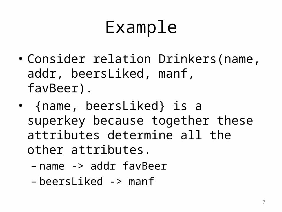
• Consider relation Drinkers(name, addr, beersLiked, manf, favBeer).
• {name, beersLiked} is a superkey because together these attributes determine all the other attributes.– name -> addr favBeer– beersLiked -> manf
7
Example
8
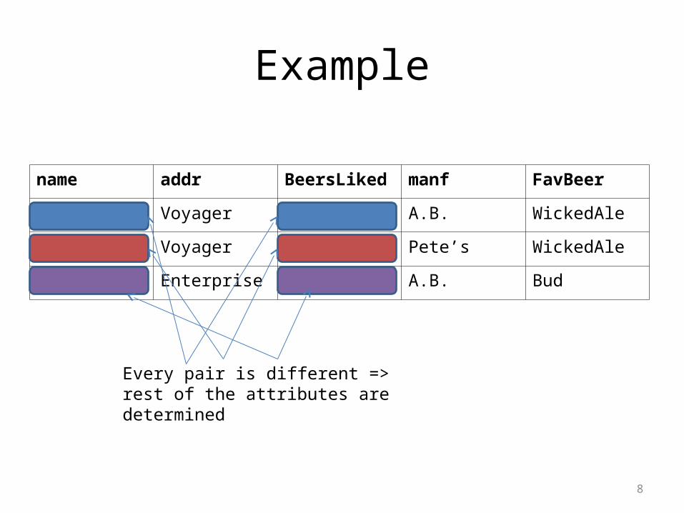
name addr BeersLiked manf FavBeer
Janeway Voyager Bud A.B. WickedAle
Janeway Voyager WickedAle Pete’s WickedAle
Spock Enterprise Bud A.B. Bud
Every pair is different => rest of the attributes are determined
Example, Cont.
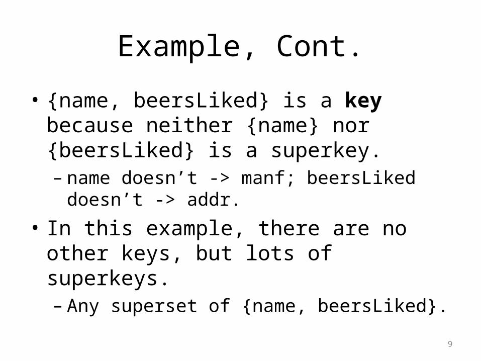
• {name, beersLiked} is a key because neither {name} nor {beersLiked} is a superkey.– name doesn’t -> manf; beersLiked doesn’t -> addr.
• In this example, there are no other keys, but lots of superkeys.– Any superset of {name, beersLiked}.
9
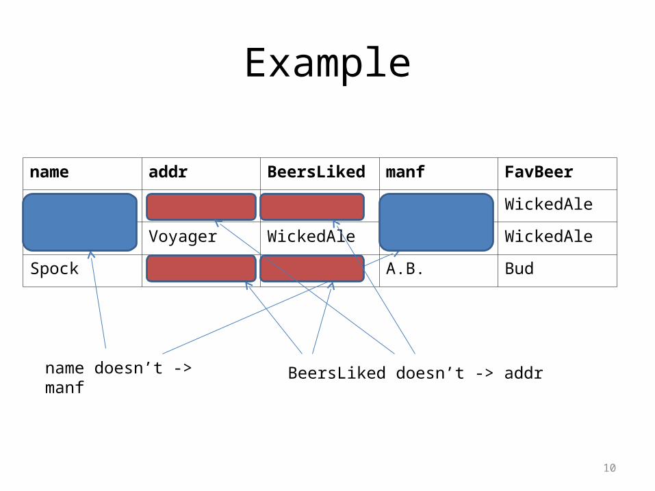
Example
10
name addr BeersLiked manf FavBeer
Janeway Voyager Bud A.B. WickedAle
Janeway Voyager WickedAle Pete’s WickedAle
Spock Enterprise Bud A.B. Bud
name doesn’t -> manf BeersLiked doesn’t -> addr
E/R and Relational Keys
• Keys in E/R are properties of entities• Keys in relations are properties of tuples.• Usually, one tuple corresponds to one entity,
so the ideas are the same.• But --- in poor relational designs, one entity
can become several tuples, so E/R keys and Relational keys are different.
11

Example
12
name addr BeersLiked manf FavBeer
Janeway Voyager Bud A.B. WickedAle
Janeway Voyager WickedAle Pete’s WickedAle
Spock Enterprise Bud A.B. Bud
name addr
Janeway Voyager
Spock Enterprise
beer manf
Bud A.B.
WickedAle Pete’s
Beers Drinkers
name, Beersliked relational key
In E/R name is a key for Drinkers, and beersLiked is a key for Beers
Where Do Keys Come From?
1. We could simply assert a key K. Then the only FD’s are K -> A for all atributes A, and K turns out to be the only key obtainable from the FD’s.
2. We could assert FD’s and deduce the keys by systematic exploration.
E/R gives us FD’s from entity-set keys and many-one relationships.
13
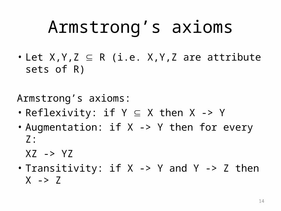
Armstrong’s axioms
• Let X,Y,Z R (i.e. X,Y,Z are attribute sets of R)
Armstrong’s axioms:• Reflexivity: if Y X then X -> Y• Augmentation: if X -> Y then for every Z:
XZ -> YZ• Transitivity: if X -> Y and Y -> Z then X -> Z
14
FD’s From “Physics”
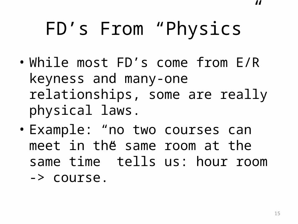
• While most FD’s come from E/R keyness and many-one relationships, some are really physical laws.
• Example: “no two courses can meet in the same room at the same time” tells us: hour room -> course.
15
Inferring FD’s: Motivation
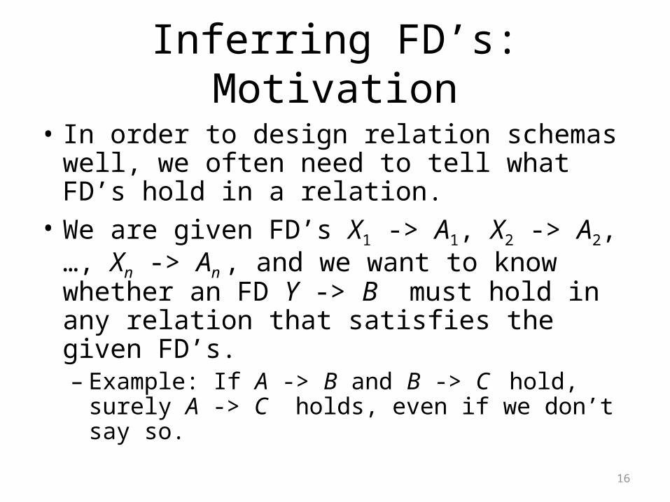
• In order to design relation schemas well, we often need to tell what FD’s hold in a relation.
• We are given FD’s X1 -> A1, X2 -> A2,…, Xn -> An , and we want to know whether an FD Y -> B must hold in any relation that satisfies the given FD’s.– Example: If A -> B and B -> C hold, surely A -> C
holds, even if we don’t say so.
16
Inference Test
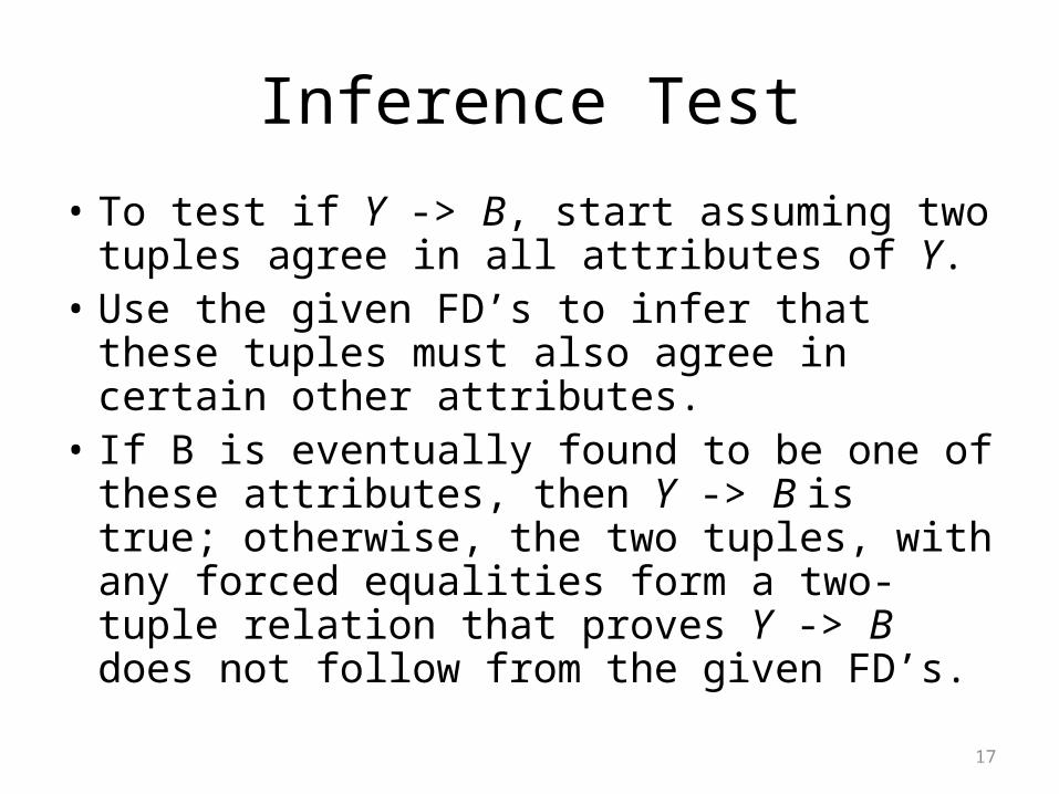
• To test if Y -> B, start assuming two tuples agree in all attributes of Y.
• Use the given FD’s to infer that these tuples must also agree in certain other attributes.
• If B is eventually found to be one of these attributes, then Y -> B is true; otherwise, the two tuples, with any forced equalities form a two-tuple relation that proves Y -> B does not follow from the given FD’s.
17
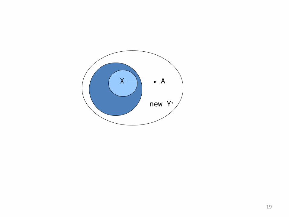
Closure Test
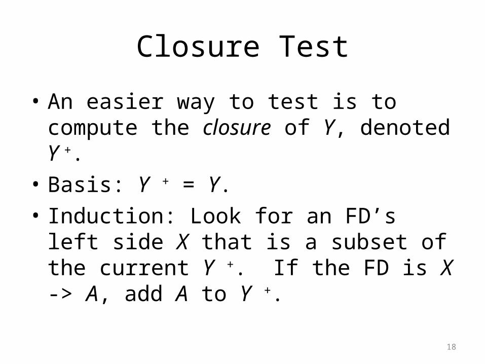
• An easier way to test is to compute the closure of Y, denoted Y +.
• Basis: Y + = Y.• Induction: Look for an FD’s left side X that is a
subset of the current Y +. If the FD is X -> A, add A to Y +.
18
19
Y+
new Y+
X A
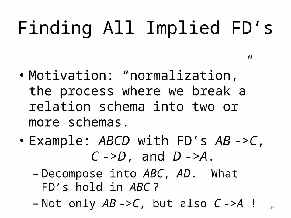
Finding All Implied FD’s
• Motivation: “normalization,” the process where we break a relation schema into two or more schemas.
• Example: ABCD with FD’s AB ->C, C ->D, and D ->A.– Decompose into ABC, AD. What FD’s hold in
ABC ?– Not only AB ->C, but also C ->A !
20
Basic Idea
• To know what FD’s hold in a projection, we start with given FD’s and find all FD’s that follow from given ones.
• Then, restrict to those FD’s that involve only attributes of the projected schema.
21
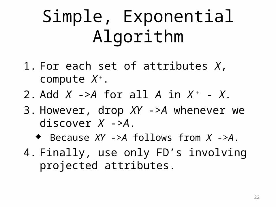
Simple, Exponential Algorithm
1. For each set of attributes X, compute X +.2. Add X ->A for all A in X + - X.3. However, drop XY ->A whenever we
discover X ->A. Because XY ->A follows from X ->A.
4. Finally, use only FD’s involving projected attributes.
22

A Few Tricks
• Never need to compute the closure of the empty set or of the set of all attributes:– ∅ += ∅– R + =R
• If we find X + = all attributes, don’t bother computing the closure of any supersets of X:– X + = R and X Y => Y + = R
23
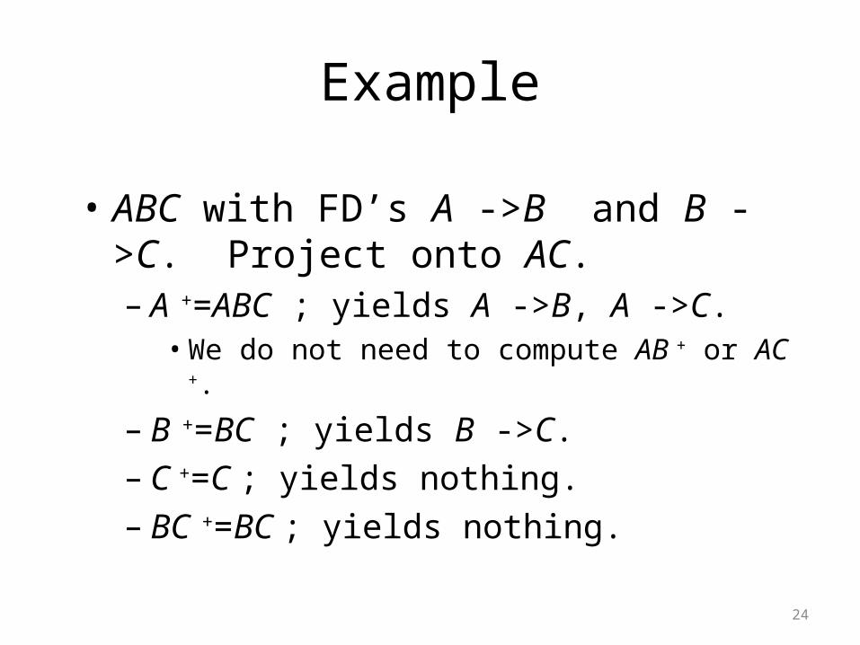
Example
• ABC with FD’s A ->B and B ->C. Project onto AC.– A +=ABC ; yields A ->B, A ->C.
• We do not need to compute AB + or AC +.
– B +=BC ; yields B ->C.– C +=C ; yields nothing.– BC +=BC ; yields nothing.
24
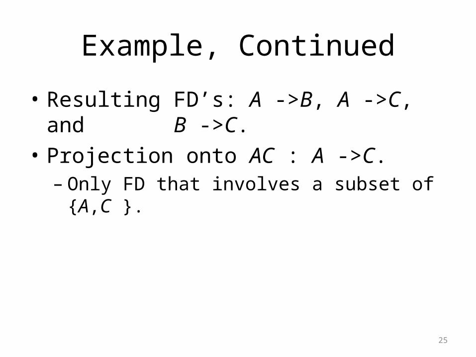
Example, Continued
• Resulting FD’s: A ->B, A ->C, and B ->C.• Projection onto AC : A ->C.
– Only FD that involves a subset of {A,C }.
25
A Geometric View of FD’s
• Imagine the set of all instances of a particular relation.
• That is, all finite sets of tuples that have the proper number of components.
• Each instance is a point in this space.
26
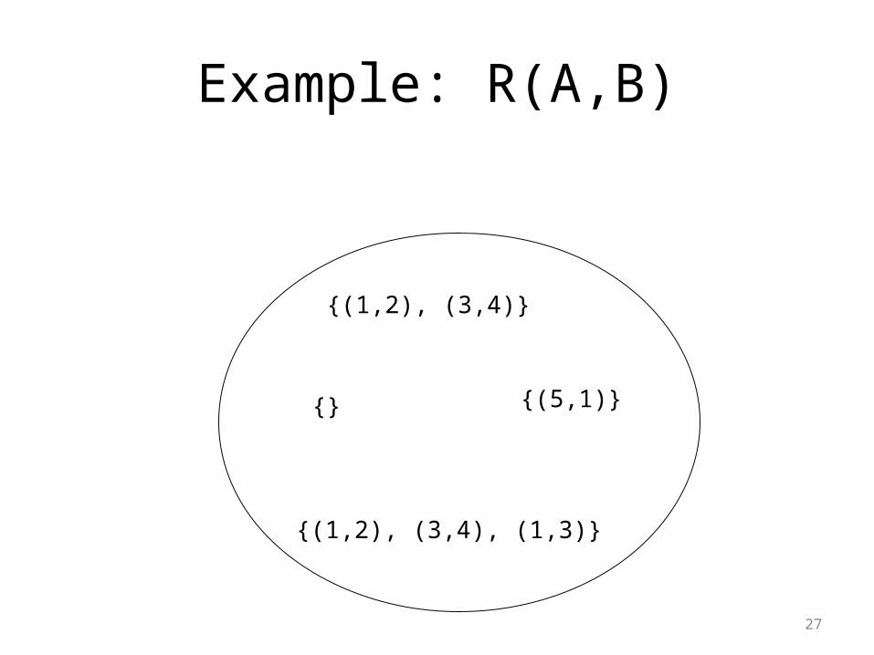
Example: R(A,B)
27
{(1,2), (3,4)}
{}
{(1,2), (3,4), (1,3)}
{(5,1)}
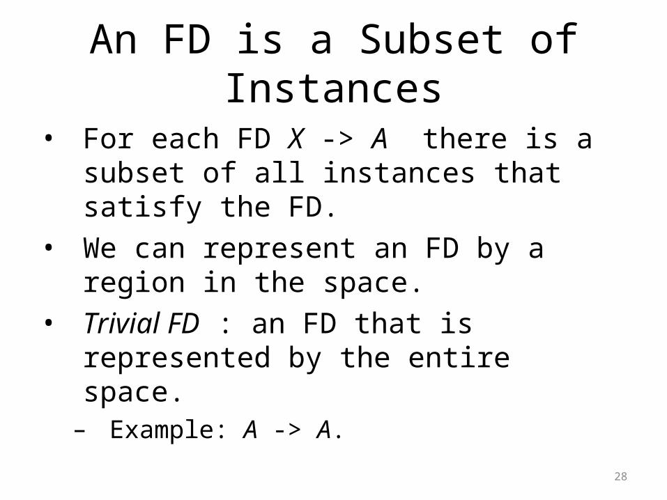
An FD is a Subset of Instances
• For each FD X -> A there is a subset of all instances that satisfy the FD.
• We can represent an FD by a region in the space.
• Trivial FD : an FD that is represented by the entire space.
– Example: A -> A.
28
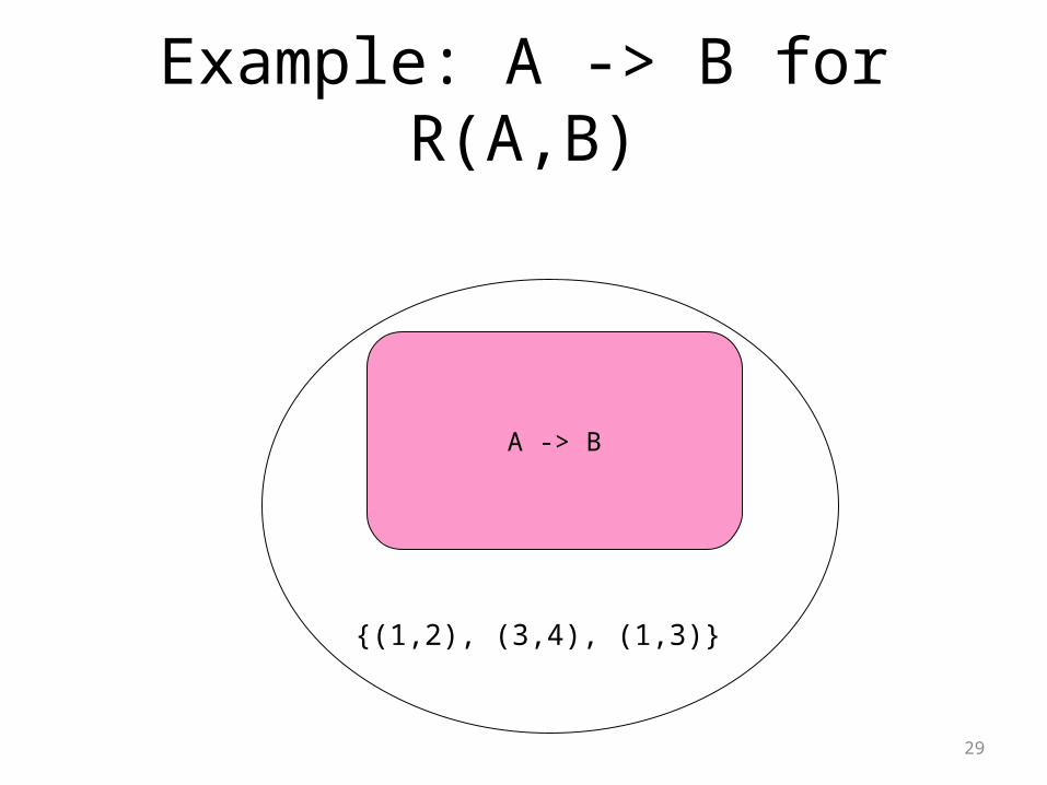
Example: A -> B for R(A,B)
29
{(1,2), (3,4)}
{}
{(1,2), (3,4), (1,3)}
{(5,1)}A -> B
Representing Sets of FD’s
• If each FD is a set of relation instances, then a collection of FD’s corresponds to the intersection of those sets.– Intersection = all instances that satisfy all of the
FD’s.
30

Example
31
A->B
B->C
CD->A
Instances satisfyingA->B, B->C, andCD->A
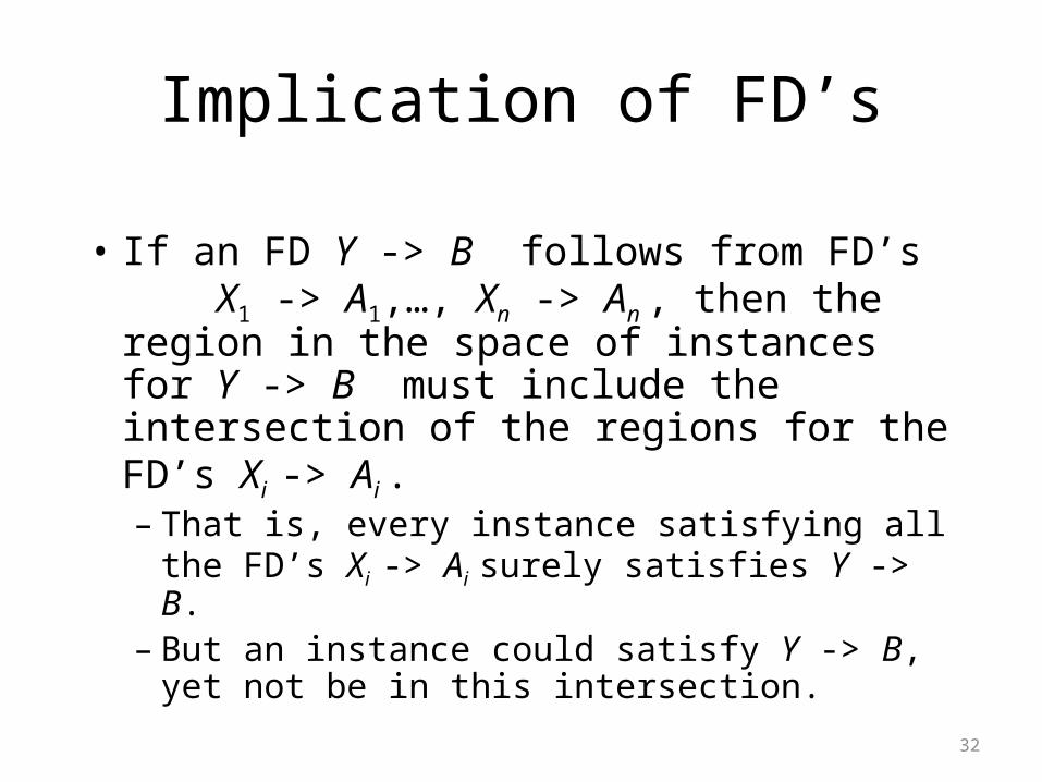
Implication of FD’s
• If an FD Y -> B follows from FD’s X1 -> A1,…, Xn -> An , then the region in the space of instances for Y -> B must include the intersection of the regions for the FD’s Xi -> Ai .– That is, every instance satisfying all the FD’s Xi -
> Ai surely satisfies Y -> B.– But an instance could satisfy Y -> B, yet not be
in this intersection.32

Example
33
A->B B->CA->C
34
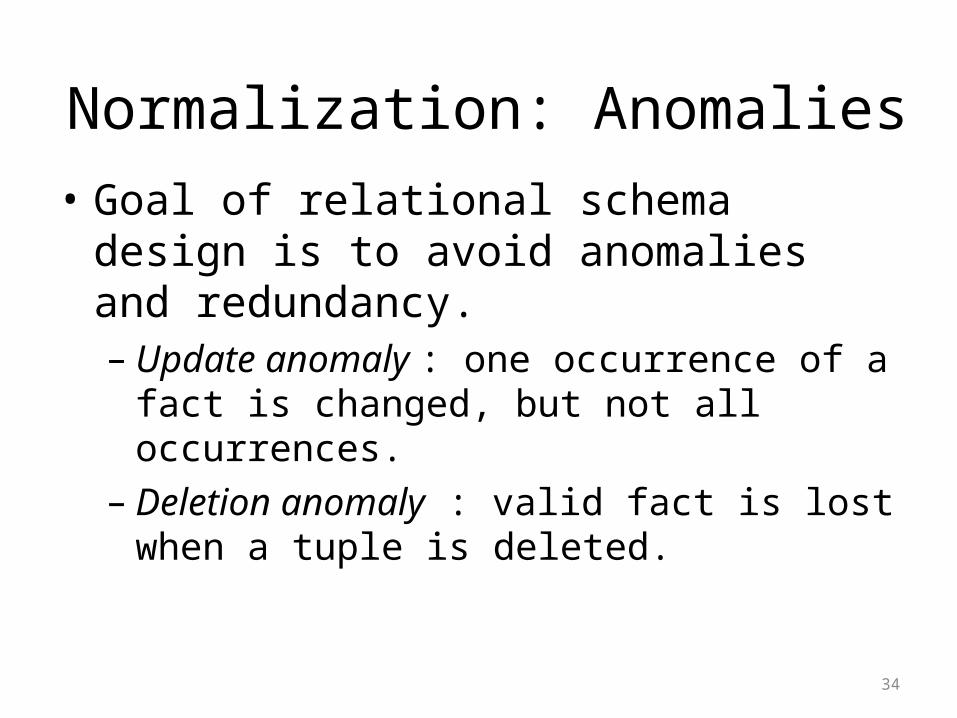
Normalization: Anomalies• Goal of relational schema design is to avoid
anomalies and redundancy.– Update anomaly : one occurrence of a fact is
changed, but not all occurrences.– Deletion anomaly : valid fact is lost when a tuple is
deleted.
35
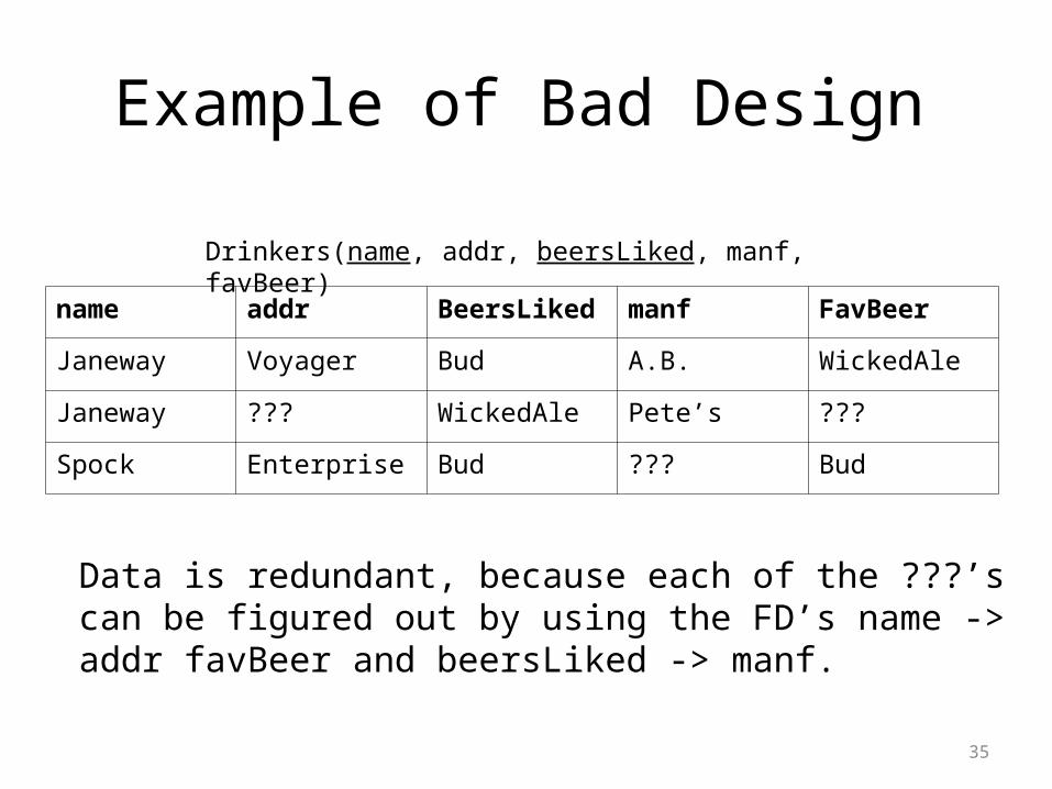
Example of Bad Design
Data is redundant, because each of the ???’s can be figured out by using the FD’s name -> addr favBeer and beersLiked -> manf.
name addr BeersLiked manf FavBeer
Janeway Voyager Bud A.B. WickedAle
Janeway ??? WickedAle Pete’s ???
Spock Enterprise Bud ??? Bud
Drinkers(name, addr, beersLiked, manf, favBeer)
36
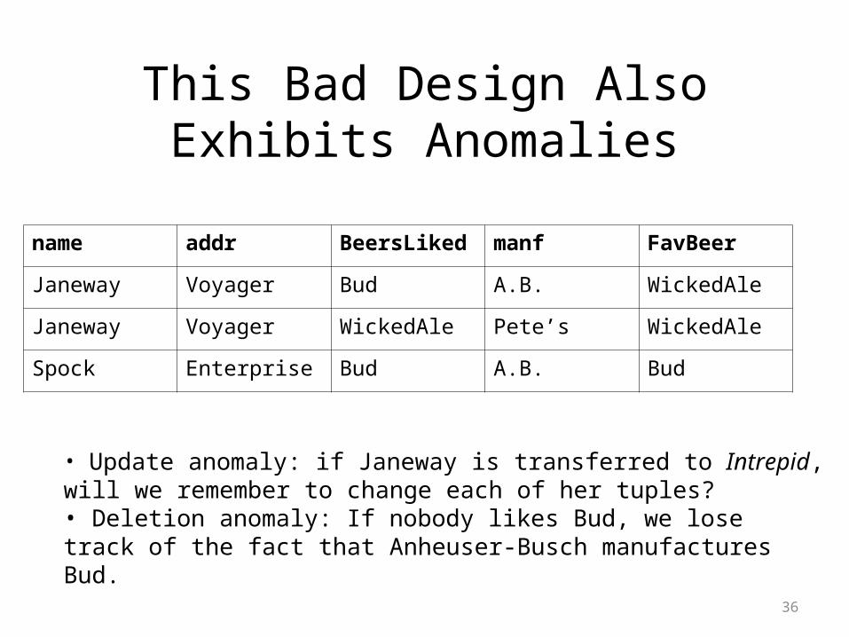
This Bad Design AlsoExhibits Anomalies
• Update anomaly: if Janeway is transferred to Intrepid, will we remember to change each of her tuples?• Deletion anomaly: If nobody likes Bud, we lose track of the fact that Anheuser-Busch manufactures Bud.
name addr BeersLiked manf FavBeer
Janeway Voyager Bud A.B. WickedAle
Janeway Voyager WickedAle Pete’s WickedAle
Spock Enterprise Bud A.B. Bud

37
Boyce-Codd Normal Form
• We say a relation R is in BCNF : if whenever X ->A is a nontrivial FD that holds in R, X is a superkey.– Remember: nontrivial means A is not a member
of set X.– Remember, a superkey is any superset of a key
(not necessarily a proper superset).
38
Example
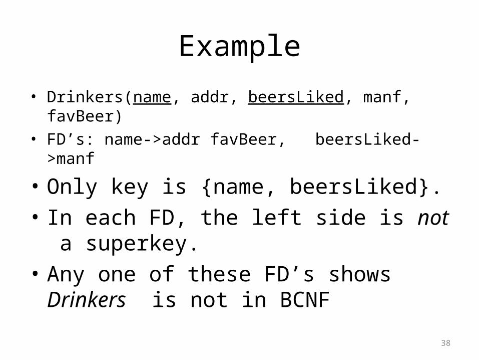
• Drinkers(name, addr, beersLiked, manf, favBeer)• FD’s: name->addr favBeer, beersLiked->manf
• Only key is {name, beersLiked}.• In each FD, the left side is not a superkey.• Any one of these FD’s shows Drinkers is not in
BCNF
39
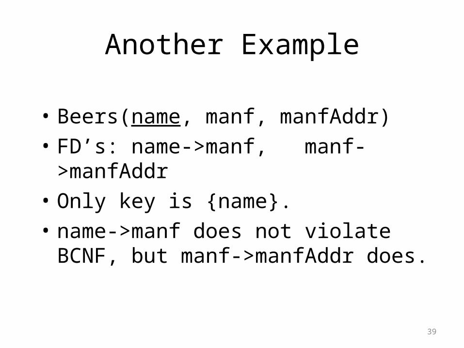
Another Example
• Beers(name, manf, manfAddr)• FD’s: name->manf, manf->manfAddr• Only key is {name}.• name->manf does not violate BCNF, but
manf->manfAddr does.
40
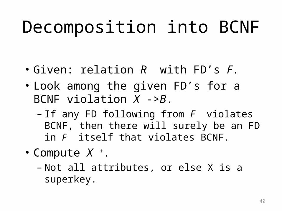
Decomposition into BCNF
• Given: relation R with FD’s F.• Look among the given FD’s for a BCNF
violation X ->B.– If any FD following from F violates BCNF, then
there will surely be an FD in F itself that violates BCNF.
• Compute X +.– Not all attributes, or else X is a superkey.
41
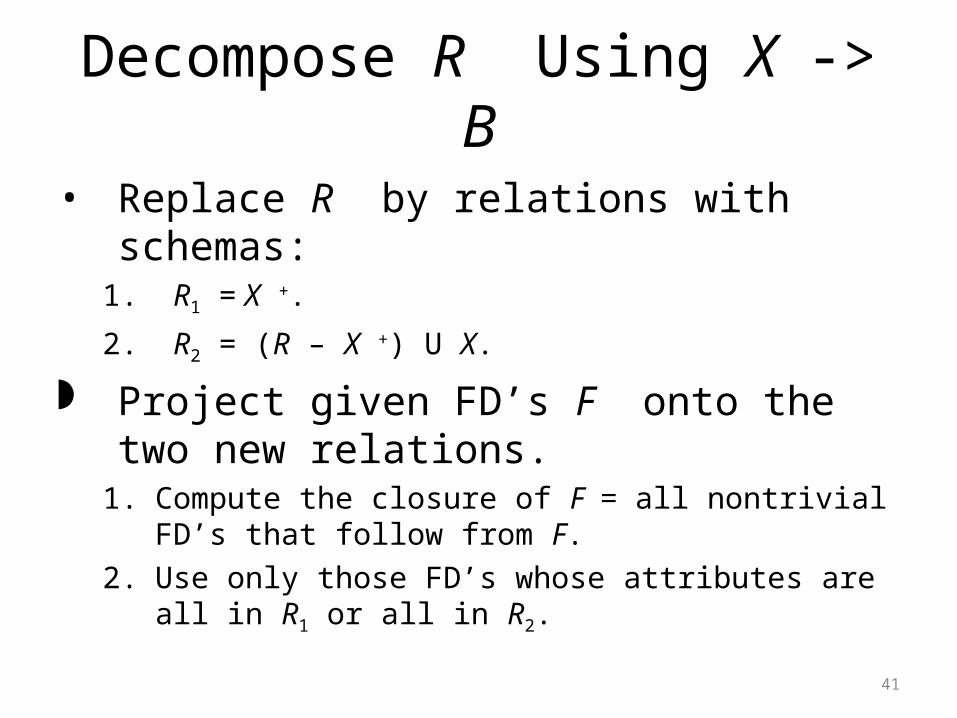
Decompose R Using X -> B
• Replace R by relations with schemas:1. R1 = X +.
2. R2 = (R – X +) U X.
Project given FD’s F onto the two new relations.
1. Compute the closure of F = all nontrivial FD’s that follow from F.
2. Use only those FD’s whose attributes are all in R1 or all in R2.
42
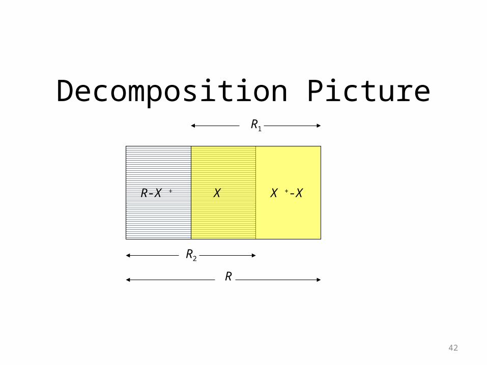
Decomposition Picture
R-X + X X +-X
R2
R1
R
43
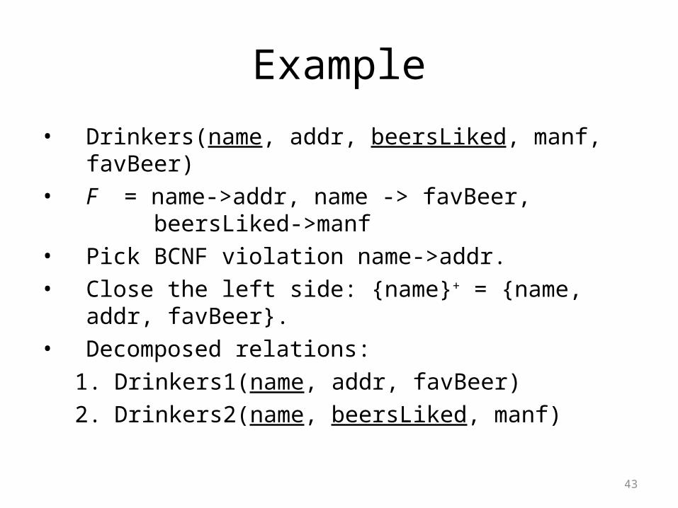
Example
• Drinkers(name, addr, beersLiked, manf, favBeer)• F = name->addr, name -> favBeer, beersLiked->manf• Pick BCNF violation name->addr.• Close the left side: {name}+ = {name, addr, favBeer}.• Decomposed relations:
1. Drinkers1(name, addr, favBeer)2. Drinkers2(name, beersLiked, manf)

44
Example, Continued
• We are not done; we need to check Drinkers1 and Drinkers2 for BCNF.
• Projecting FD’s is complex in general, easy here.
• For Drinkers1(name, addr, favBeer), relevant FD’s are name->addr and name->favBeer.– Thus, name is the only key and Drinkers1 is in BCNF.
45
Example, Continued
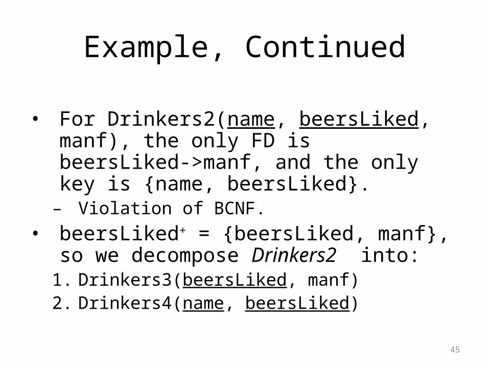
• For Drinkers2(name, beersLiked, manf), the only FD is beersLiked->manf, and the only key is {name, beersLiked}.
– Violation of BCNF.• beersLiked+ = {beersLiked, manf}, so we
decompose Drinkers2 into:1. Drinkers3(beersLiked, manf)2. Drinkers4(name, beersLiked)
46
Example, Concluded
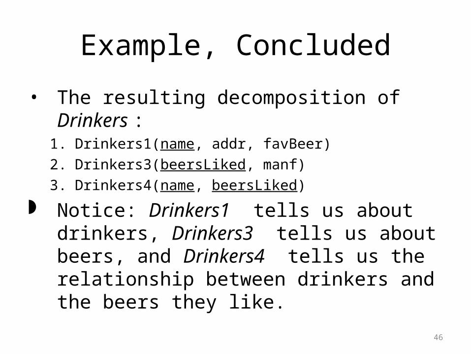
• The resulting decomposition of Drinkers :1. Drinkers1(name, addr, favBeer)2. Drinkers3(beersLiked, manf)3. Drinkers4(name, beersLiked)
Notice: Drinkers1 tells us about drinkers, Drinkers3 tells us about beers, and Drinkers4 tells us the relationship between drinkers and the beers they like.
47
Third Normal Form - Motivation
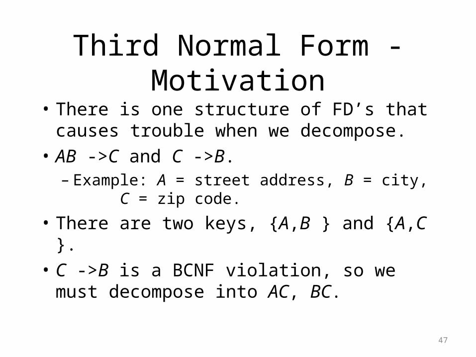
• There is one structure of FD’s that causes trouble when we decompose.
• AB ->C and C ->B.– Example: A = street address, B = city, C = zip
code.
• There are two keys, {A,B } and {A,C }.• C ->B is a BCNF violation, so we must
decompose into AC, BC.
48
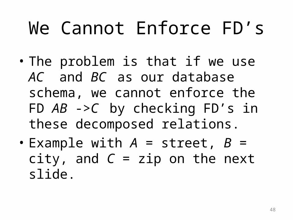
We Cannot Enforce FD’s
• The problem is that if we use AC and BC as our database schema, we cannot enforce the FD AB ->C by checking FD’s in these decomposed relations.
• Example with A = street, B = city, and C = zip on the next slide.

49
An Unenforceable FD street zip
545 Tech Sq. 02138545 Tech Sq. 02139
city zip
Cambridge 02138Cambridge 02139
Join tuples with equal zip codes.
street city zip
545 Tech Sq. Cambridge 02138545 Tech Sq. Cambridge 02139
Although no FD’s were violated in the decomposed relations,FD street city -> zip is violated by the database as a whole.
50
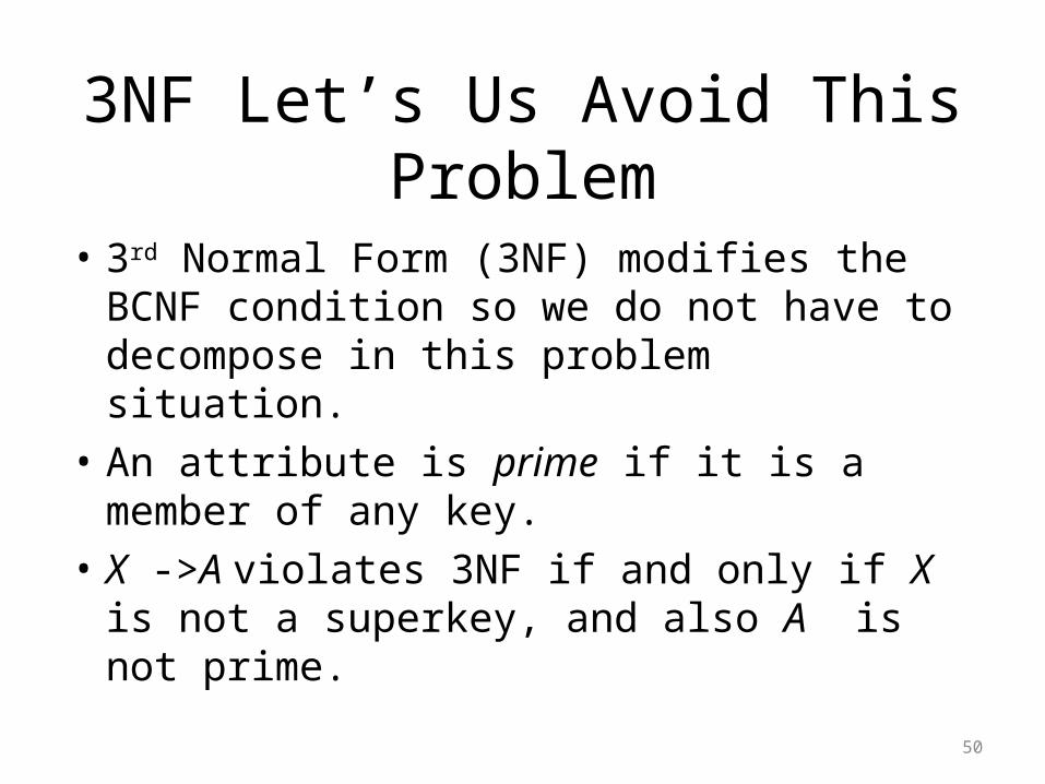
3NF Let’s Us Avoid This Problem
• 3rd Normal Form (3NF) modifies the BCNF condition so we do not have to decompose in this problem situation.
• An attribute is prime if it is a member of any key.
• X ->A violates 3NF if and only if X is not a superkey, and also A is not prime.
51
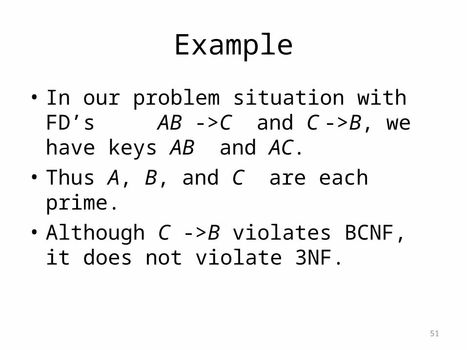
Example
• In our problem situation with FD’s AB ->C and C ->B, we have keys AB and AC.
• Thus A, B, and C are each prime.• Although C ->B violates BCNF, it does not
violate 3NF.
52
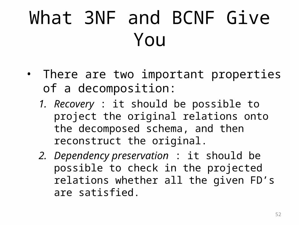
What 3NF and BCNF Give You
• There are two important properties of a decomposition:
1. Recovery : it should be possible to project the original relations onto the decomposed schema, and then reconstruct the original.
2. Dependency preservation : it should be possible to check in the projected relations whether all the given FD’s are satisfied.
53
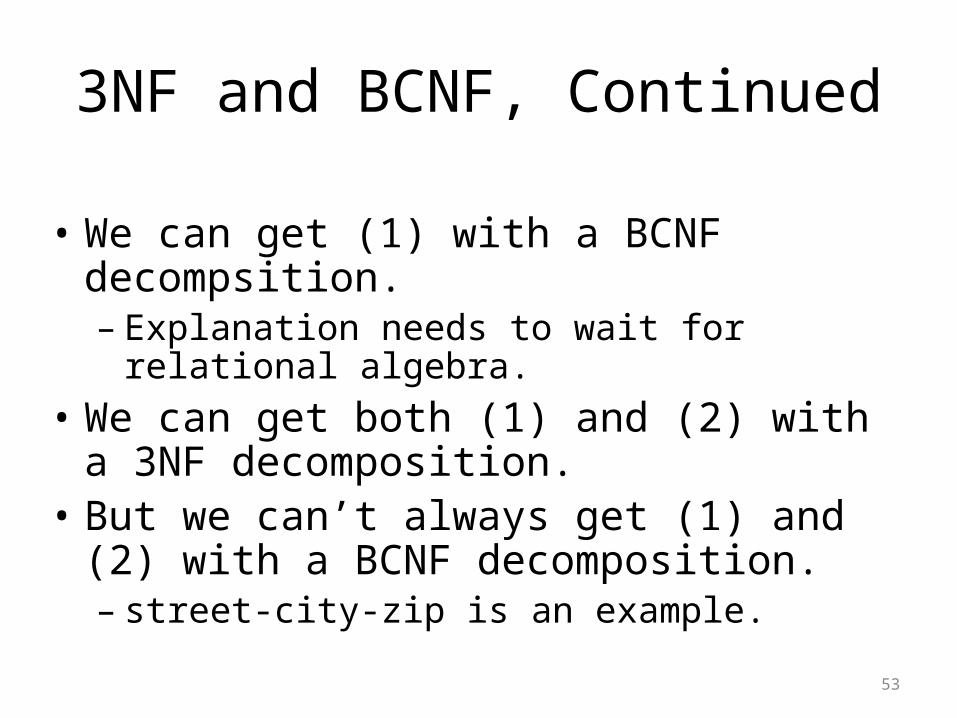
3NF and BCNF, Continued
• We can get (1) with a BCNF decompsition.– Explanation needs to wait for relational algebra.
• We can get both (1) and (2) with a 3NF decomposition.
• But we can’t always get (1) and (2) with a BCNF decomposition.– street-city-zip is an example.
54
A New Form of Redundancy
• Multivalued dependencies (MVD’s) express a condition among tuples of a relation that exists when the relation is trying to represent more than one many-many relationship.
• Then certain attributes become independent of one another, and their values must appear in all combinations.
55
Example
Drinkers(name, addr, phones, beersLiked)• A drinker’s phones are independent of the beers
they like.• Thus, each of a drinker’s phones appears with
each of the beers they like in all combinations.• This repetition is unlike redundancy due to FD’s,
of which name->addr is the only one.
56
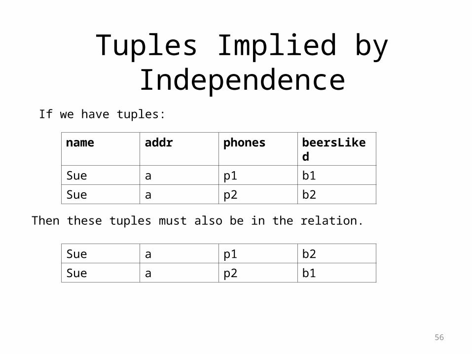
Tuples Implied by Independence
If we have tuples:
Then these tuples must also be in the relation.
name addr phones beersLiked
Sue a p1 b1
Sue a p2 b2
Sue a p1 b2
Sue a p2 b1
57
Definition of MVD
• A multivalued dependency (MVD) X ->->Y is an assertion that if two tuples of a relation agree on all the attributes of X, then their components in the set of attributes Y may be swapped, and the result will be two tuples that are also in the relation.
58
Example
• The name-addr-phones-beersLiked example illustrated the MVD
name->->phones and the MVD
name ->-> beersLiked.
59
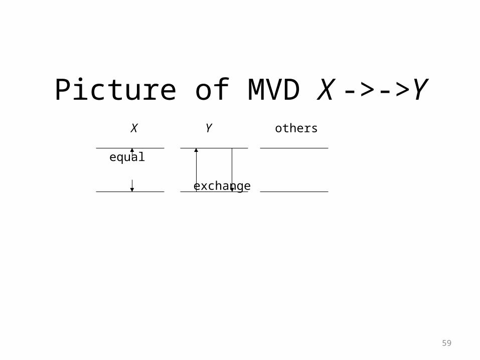
Picture of MVD X ->->Y X Y others
equal
exchange
60
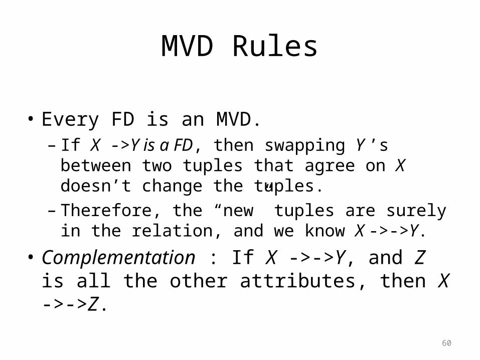
MVD Rules
• Every FD is an MVD.– If X ->Y is a FD, then swapping Y ’s between two
tuples that agree on X doesn’t change the tuples.– Therefore, the “new” tuples are surely in the
relation, and we know X ->->Y.
• Complementation : If X ->->Y, and Z is all the other attributes, then X ->->Z.

61
Splitting Doesn’t Hold
• Like FD’s, we cannot generally split the left side of an MVD.
• But unlike FD’s, we cannot split the right side either --- sometimes you have to leave several attributes on the right side.

62
Example
• Consider a drinkers relation:Drinkers(name, areaCode, phone, beersLiked,
manf)• A drinker can have several phones, with the
number divided between areaCode and phone (last 7 digits).
• A drinker can like several beers, each with its own manufacturer.
63
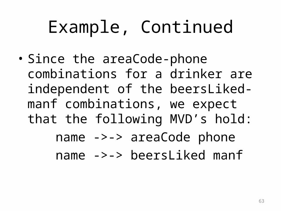
Example, Continued
• Since the areaCode-phone combinations for a drinker are independent of the beersLiked-manf combinations, we expect that the following MVD’s hold:
name ->-> areaCode phonename ->-> beersLiked manf
64
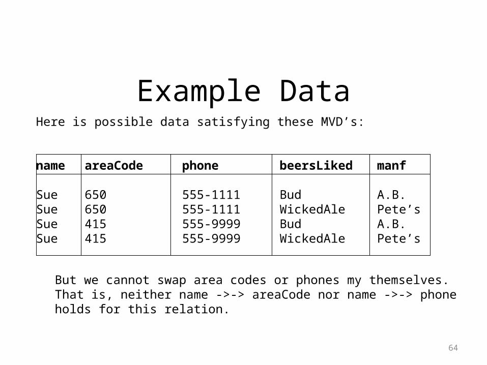
Example DataHere is possible data satisfying these MVD’s:
name areaCode phone beersLiked manf
Sue 650 555-1111 Bud A.B.Sue 650 555-1111 WickedAle Pete’sSue 415 555-9999 Bud A.B.Sue 415 555-9999 WickedAle Pete’s
But we cannot swap area codes or phones my themselves.That is, neither name ->-> areaCode nor name ->-> phoneholds for this relation.
65
Fourth Normal Form
• The redundancy that comes from MVD’s is not removable by putting the database schema in BCNF.
• There is a stronger normal form, called 4NF, that (intuitively) treats MVD’s as FD’s when it comes to decomposition, but not when determining keys of the relation.

66
4NF Definition
• A relation R is in 4NF if whenever X ->->Y is a nontrivial MVD, then X is a superkey.
– “Nontrivial means that:1. Y is not a subset of X, and2. X and Y are not, together, all the attributes.
– Note that the definition of “superkey” still depends on FD’s only.
67
BCNF Versus 4NF
• Remember that every FD X ->Y is also an MVD, X ->->Y.
• Thus, if R is in 4NF, it is certainly in BCNF.– Because any BCNF violation is a 4NF violation.
• But R could be in BCNF and not 4NF, because MVD’s are “invisible” to BCNF.
68
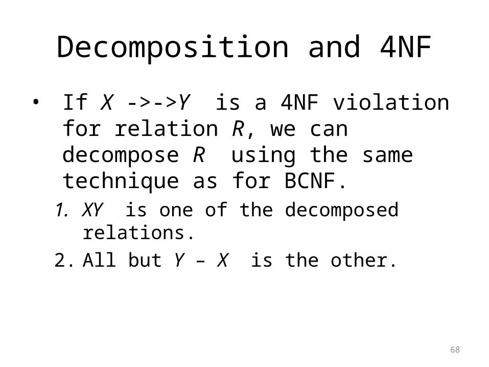
Decomposition and 4NF
• If X ->->Y is a 4NF violation for relation R, we can decompose R using the same technique as for BCNF.
1. XY is one of the decomposed relations.2. All but Y – X is the other.
69
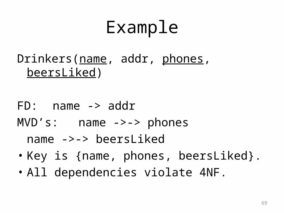
Example
Drinkers(name, addr, phones, beersLiked)
FD: name -> addrMVD’s: name ->-> phones
name ->-> beersLiked• Key is {name, phones, beersLiked}.• All dependencies violate 4NF.
70
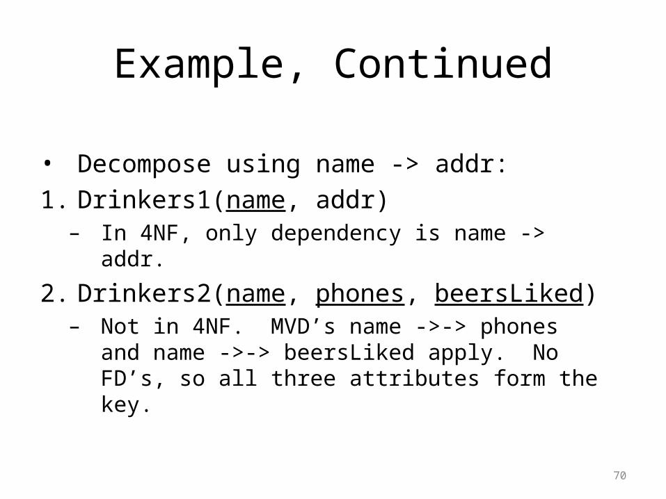
Example, Continued
• Decompose using name -> addr:1. Drinkers1(name, addr)
– In 4NF, only dependency is name -> addr.
2. Drinkers2(name, phones, beersLiked)– Not in 4NF. MVD’s name ->-> phones and
name ->-> beersLiked apply. No FD’s, so all three attributes form the key.
71
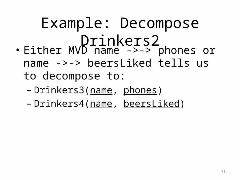
Example: Decompose Drinkers2• Either MVD name ->-> phones or name ->->
beersLiked tells us to decompose to:– Drinkers3(name, phones)– Drinkers4(name, beersLiked)

On-Line Application Processing
• Warehousing• Data Cubes• Data Mining
72
73
Overview
• Traditional database systems are tuned to many, small, simple queries.
• Some new applications use fewer, more time-consuming, complex queries.
• New architectures have been developed to handle complex “analytic” queries efficiently.
74
The Data Warehouse
• The most common form of data integration.– Copy sources into a single DB (warehouse) and try
to keep it up-to-date.– Usual method: periodic reconstruction of the
warehouse, perhaps overnight.– Frequently essential for analytic queries.
75
OLTP
• Most database operations involve On-Line Transaction Processing (OTLP).– Short, simple, frequent queries and/or
modifications, each involving a small number of tuples.
– Examples: • Answering queries from a Web interface• Sales at cash registers • Selling airline tickets
76
OLAP
• Of increasing importance are On-Line Analytical Processing (OLAP) queries.– Few, but complex queries --- may run for hours.– Queries do not depend on having an absolutely
up-to-date database.
• Sometimes called Data Mining.

77
OLAP Examples
1. Amazon analyzes purchases by its customers to come up with an individual screen with products of likely interest to the customer.
2. Analysts at Wal-Mart look for items with increasing sales in some region.
78
Common Architecture
• Databases at store branches handle OLTP.• Local store databases copied to a central
warehouse overnight.• Analysts use the warehouse for OLAP.
79
Star Schemas
• A star schema is a common organization for data at a warehouse. It consists of:
1. Fact table : a very large accumulation of facts such as sales. Often “insert-only.”
2. Dimension tables : smaller, generally static information about the entities involved in the facts.
80
Example: Star Schema
• Suppose we want to record in a warehouse information about every beer sale: the bar, the brand of beer, the drinker who bought the beer, the day, the time, and the price charged.
• The fact table is a relation:Sales(bar, beer, drinker, day, time, price)
81
Example, Continued
• The dimension tables include information about the bar, beer, and drinker “dimensions”:
Bars(bar, addr, license)Beers(beer, manf)Drinkers(drinker, addr, phone)
82
Dimensions and Dependent Attributes
• Two classes of fact-table attributes:1. Dimension attributes : the key of a dimension
table.2. Dependent attributes : a value determined by
the dimension attributes of the tuple.
83
Example: Dependent Attribute
• price is the dependent attribute of our example Sales relation.
• It is determined by the combination of dimension attributes: bar, beer, drinker, and the time (combination of day and time attributes).
84
Approaches to Building Warehouses
1. ROLAP = “relational OLAP”: Tune a relational DBMS to support star schemas.
2. MOLAP = “multidimensional OLAP”: Use a specialized DBMS with a model such as the “data cube.”
85
ROLAP Techniques
1. Bitmap indexes : For each key value of a dimension table (e.g., each beer for relation Beers) create a bit-vector telling which tuples of the fact table have that value.
2. Materialized views : Store the answers to several useful queries (views) in the warehouse itself.
86
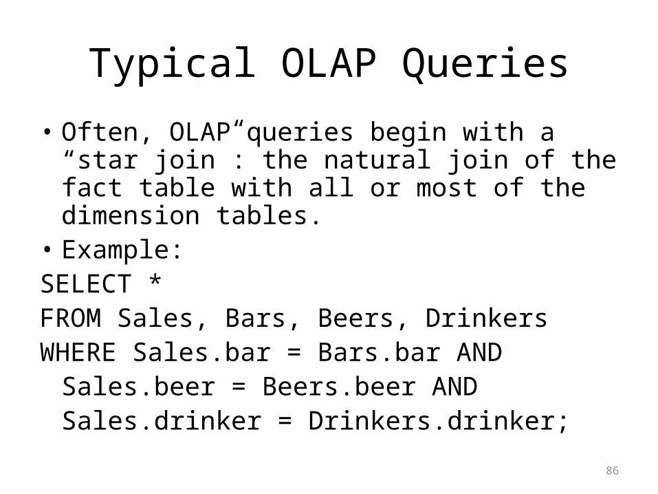
Typical OLAP Queries
• Often, OLAP queries begin with a “star join”: the natural join of the fact table with all or most of the dimension tables.
• Example:SELECT *FROM Sales, Bars, Beers, DrinkersWHERE Sales.bar = Bars.bar ANDSales.beer = Beers.beer ANDSales.drinker = Drinkers.drinker;
87
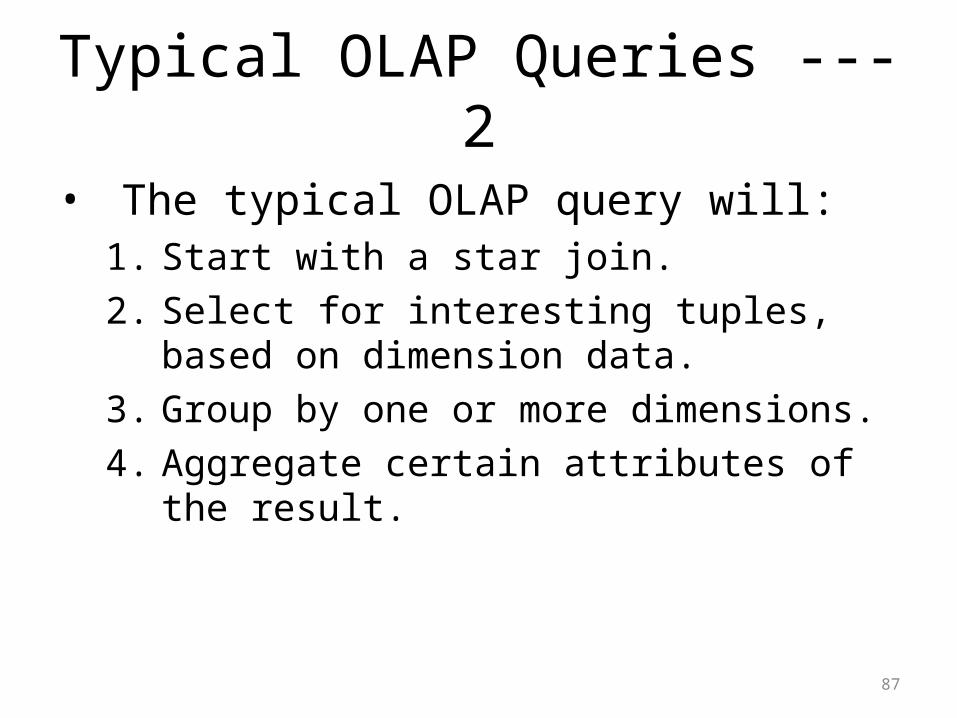
Typical OLAP Queries --- 2
• The typical OLAP query will:1. Start with a star join.2. Select for interesting tuples, based on dimension
data.3. Group by one or more dimensions.4. Aggregate certain attributes of the result.
88
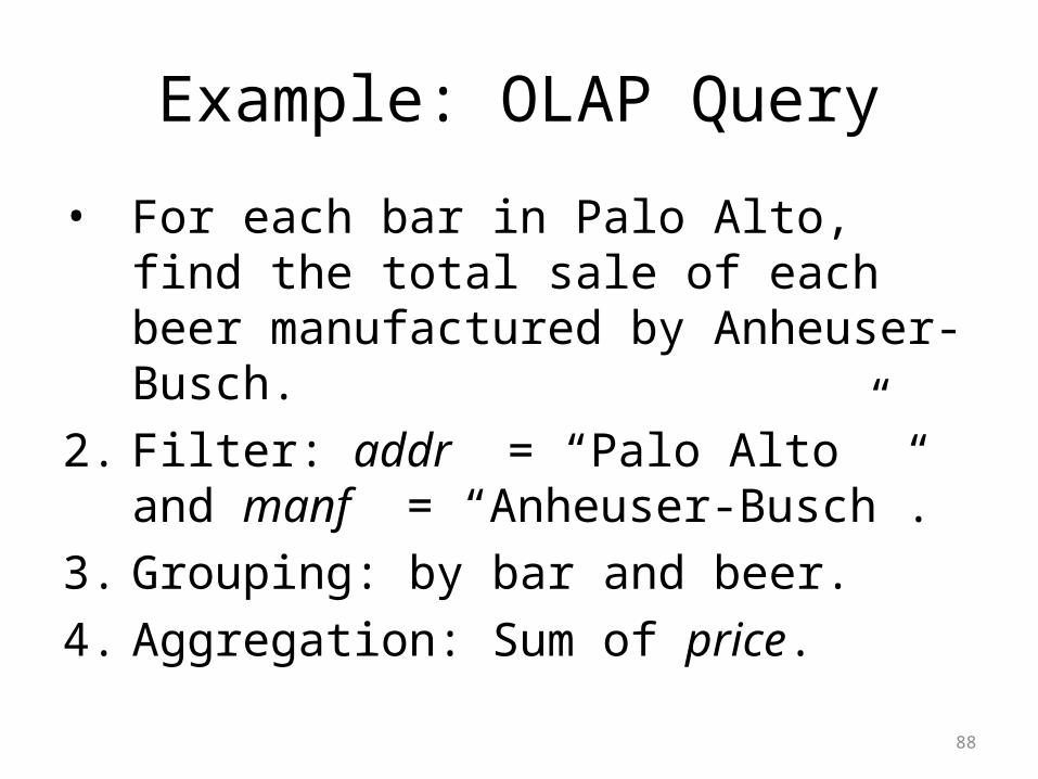
Example: OLAP Query
• For each bar in Palo Alto, find the total sale of each beer manufactured by Anheuser-Busch.
2. Filter: addr = “Palo Alto” and manf = “Anheuser-Busch”.
3. Grouping: by bar and beer.4. Aggregation: Sum of price.

89
Example: In SQL
SELECT bar, beer, SUM(price)
FROM Sales NATURAL JOIN Bars
NATURAL JOIN Beers
WHERE addr = ’Palo Alto’ AND
manf = ’Anheuser-Busch’
GROUP BY bar, beer;
90
Using Materialized Views
• A direct execution of this query from Sales and the dimension tables could take too long.
• If we create a materialized view that contains enough information, we may be able to answer our query much faster.
91
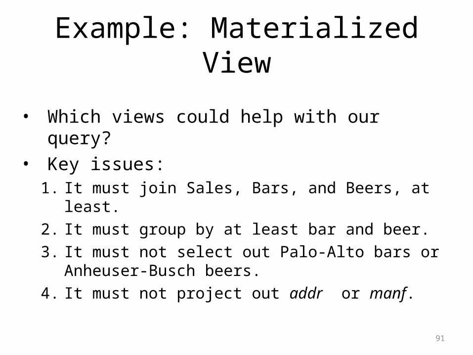
Example: Materialized View
• Which views could help with our query?• Key issues:
1. It must join Sales, Bars, and Beers, at least.2. It must group by at least bar and beer.3. It must not select out Palo-Alto bars or Anheuser-
Busch beers.4. It must not project out addr or manf.
92
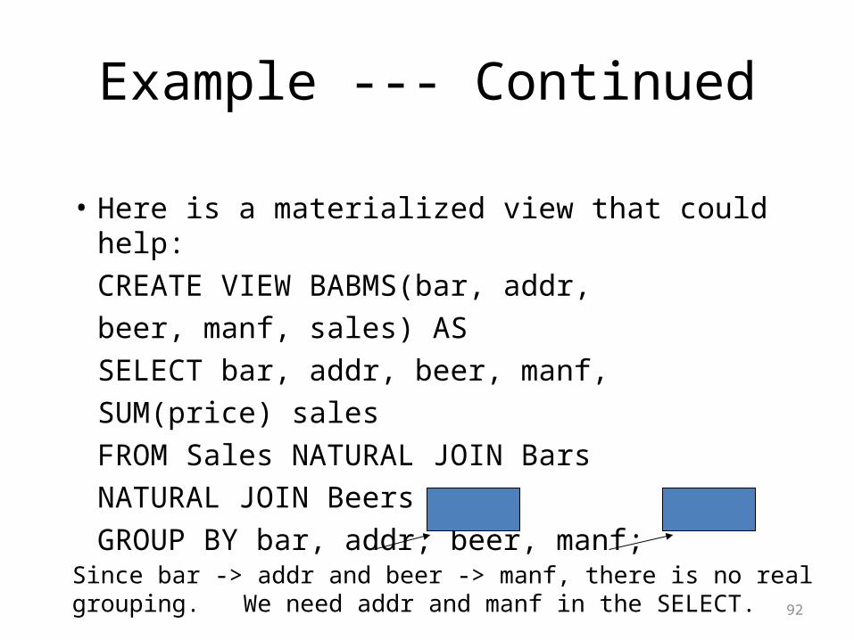
Example --- Continued
• Here is a materialized view that could help:CREATE VIEW BABMS(bar, addr,
beer, manf, sales) AS
SELECT bar, addr, beer, manf,
SUM(price) sales
FROM Sales NATURAL JOIN Bars
NATURAL JOIN Beers
GROUP BY bar, addr, beer, manf; Since bar -> addr and beer -> manf, there is no realgrouping. We need addr and manf in the SELECT.
93
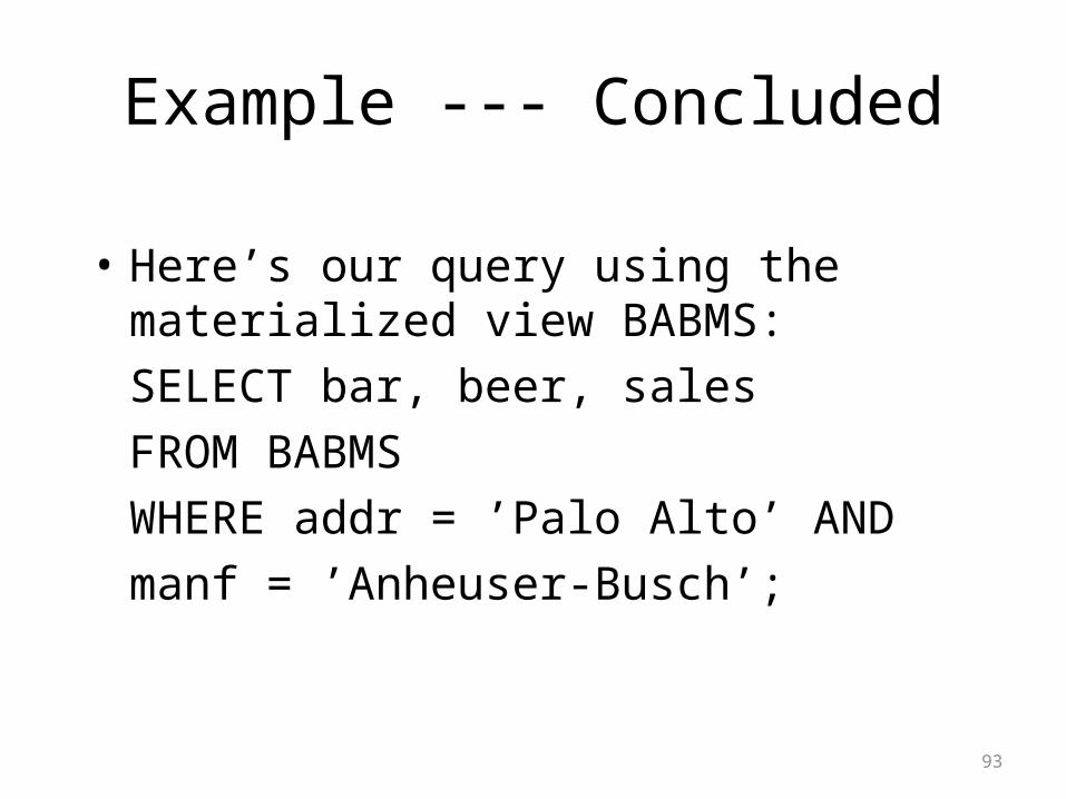
Example --- Concluded
• Here’s our query using the materialized view BABMS:
SELECT bar, beer, sales
FROM BABMS
WHERE addr = ’Palo Alto’ AND
manf = ’Anheuser-Busch’;
94
MOLAP and Data Cubes
• Keys of dimension tables are the dimensions of a hypercube.– Example: for the Sales data, the four dimensions
are bars, beers, drinkers, and time.
• Dependent attributes (e.g., price) appear at the points of the cube.
95
Marginals
• The data cube also includes aggregation (typically SUM) along the margins of the cube.
• The marginals include aggregations over one dimension, two dimensions,…
96
Example: Marginals
• Our 4-dimensional Sales cube includes the sum of price over each bar, each beer, each drinker, and each time unit (perhaps days).
• It would also have the sum of price over all bar-beer pairs, all bar-drinker-day triples,…
97
Structure of the Cube
• Think of each dimension as having an additional value *.
• A point with one or more *’s in its coordinates aggregates over the dimensions with the *’s.
• Example: Sales(“Joe’s Bar”, “Bud”, *, *) holds the sum over all drinkers and all time of the Bud consumed at Joe’s.
98
Drill-Down
• Drill-down = “de-aggregate” = break an aggregate into its constituents.
• Example: having determined that Joe’s Bar sells very few Anheuser-Busch beers, break down his sales by particular A.-B. beer.
99
Roll-Up
• Roll-up = aggregate along one or more dimensions.
• Example: given a table of how much Bud each drinker consumes at each bar, roll it up into a table giving total amount of Bud consumed for each drinker.
100
Materialized Data-Cube Views
• Data cubes invite materialized views that are aggregations in one or more dimensions.
• Dimensions may not be completely aggregated --- an option is to group by an attribute of the dimension table.
101
Example
• A materialized view for our Sales data cube might:
1. Aggregate by drinker completely.2. Not aggregate at all by beer.3. Aggregate by time according to the week.4. Aggregate according to the city of the bar.
102
Data Mining
• Data mining is a popular term for queries that summarize big data sets in useful ways.
• Examples:1. Clustering all Web pages by topic.2. Finding characteristics of fraudulent credit-card
use.
103
Market-Basket Data
• An important form of mining from relational data involves market baskets = sets of “items” that are purchased together as a customer leaves a store.
• Summary of basket data is frequent itemsets = sets of items that often appear together in baskets.
104
Example: Market Baskets
• If people often buy hamburger and ketchup together, the store can:
1. Put hamburger and ketchup near each other and put potato chips between.
2. Run a sale on hamburger and raise the price of ketchup.
105
Finding Frequent Pairs
• The simplest case is when we only want to find “frequent pairs” of items.
• Assume data is in a relation Baskets(basket, item).
• The support threshold s is the minimum number of baskets in which a pair appears before we are interested.
106
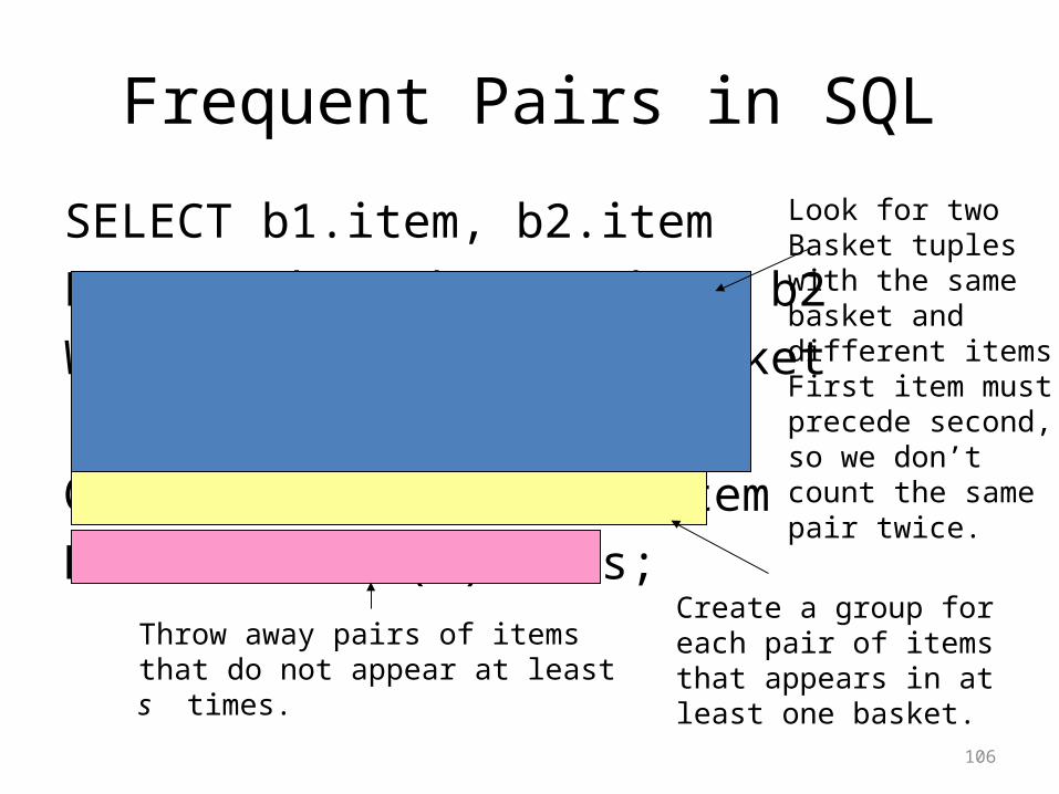
Frequent Pairs in SQL
SELECT b1.item, b2.item
FROM Baskets b1, Baskets b2
WHERE b1.basket = b2.basket
AND b1.item < b2.item
GROUP BY b1.item, b2.item
HAVING COUNT(*) >= s;
Look for twoBasket tupleswith the samebasket anddifferent items.First item mustprecede second,so we don’tcount the samepair twice.
Create a group foreach pair of itemsthat appears in atleast one basket.
Throw away pairs of itemsthat do not appear at leasts times.
107
A-Priori Trick --- 1
• Straightforward implementation involves a join of a huge Baskets relation with itself.
• The a-priori algorithm speeds the query by recognizing that a pair of items {i,j } cannot have support s unless both {i } and {j } do.

108
A-Priori Trick --- 2
• Use a materialized view to hold only information about frequent items.
INSERT INTO Baskets1(basket, item)
SELECT * FROM Baskets
WHERE item IN (
SELECT ITEM FROM Baskets
GROUP BY item
HAVING COUNT(*) >= s
);
Items thatappear in atleast s baskets.
109
A-Priori Algorithm
1. Materialize the view Baskets1.2. Run the obvious query, but on Baskets1
instead of Baskets.• Baskets1 is cheap, since it doesn’t involve
a join.• Baskets1 probably has many fewer tuples
than Baskets.– Running time shrinks with the square of the
number of tuples involved in the join.
110
Example: A-Priori
• Suppose:1. A supermarket sells 10,000 items.2. The average basket has 10 items.3. The support threshold is 1% of the baskets.
• At most 1/10 of the items can be frequent.• Probably, the minority of items in one basket
are frequent -> factor 4 speedup.