Database Theory - Lecture 11: Introduction to Datalog
48
DATABASE THEORY Lecture 11: Introduction to Datalog Markus Kr ¨ otzsch Knowledge-Based Systems TU Dresden, 12th June 2018
Transcript of Database Theory - Lecture 11: Introduction to Datalog
DATABASE THEORY
Lecture 11: Introduction to Datalog
Markus Krotzsch
Knowledge-Based Systems
TU Dresden, 12th June 2018

Announcement
All lecturesand the exerciseon 19 June 2018will be in room
APB 1004
Markus Krötzsch, 12th June 2018 Database Theory slide 2 of 34

Introduction to Datalog
Markus Krötzsch, 12th June 2018 Database Theory slide 3 of 34

Introduction to DatalogDatalog introduces recursion into database queries
• Use deterministic rules to derive new information from given facts
• Inspired by logic programming (Prolog)
• However, no function symbols and no negation
• Studied in AI (knowledge representation) and in databases (query language)
Example 11.1: Transitive closure C of a binary relation r
C(x, y)← r(x, y)
C(x, z)← C(x, y) ∧ r(y, z)
Intuition:
• some facts of the form r(x, y) are given as input, and the rules derive newconclusions C(x, y)
• variables range over all possible values (implicit universal quantifier)
Markus Krötzsch, 12th June 2018 Database Theory slide 4 of 34

Syntax of Datalog
Recall: A term is a constant or a variable. An atom is a formula of the form R(t1, . . . , tn)with R a predicate symbol (or relation) of arity n, and t1, . . . , tn terms.
Definition 11.2: A Datalog rule is an expression of the form:
H ← B1 ∧ . . . ∧ Bm
where H and B1, . . . , Bm are atoms. H is called the head or conclusion; B1 ∧ . . . ∧
Bm is called the body or premise. A rule with empty body (m = 0) is called a fact.A ground rule is one without variables (i.e., all terms are constants).
A set of Datalog rules is a Datalog program.
Markus Krötzsch, 12th June 2018 Database Theory slide 5 of 34

Datalog: Example
father(alice, bob)
mother(alice, carla)
mother(evan, carla)
father(carla, david)
Parent(x, y)← father(x, y)
Parent(x, y)← mother(x, y)
Ancestor(x, y)← Parent(x, y)
Ancestor(x, z)← Parent(x, y) ∧ Ancestor(y, z)
SameGeneration(x, x)
SameGeneration(x, y)← Parent(x, v) ∧ Parent(y, w) ∧ SameGeneration(v, w)
Markus Krötzsch, 12th June 2018 Database Theory slide 6 of 34

Datalog Semantics by Deduction
What does a Datalog program express?Usually we are interested in entailed ground atoms
What can be entailed? Informally:
• Restrict to set of constants that occur in program (finite){ universeU
• Variables can represent arbitrary constants from this set{ ground substitutions map variables to constants
• A rule can be applied if its body is satisfied for some ground substitution
Example 11.3: The rule Parent(x, y) ← mother(x, y) can be applied tomother(alice, carla) under substitution {x 7→ alice, y 7→ carla}.
• If a rule is applicable under some ground substitution, then the according instanceof the rule head is entailed.
Markus Krötzsch, 12th June 2018 Database Theory slide 7 of 34

Datalog Semantics by Deduction (2)
An inductive definition of what can be derived:
Definition 11.4: Consider a Datalog program P. The set of ground atoms thatcan be derived from P is the smallest set of atoms A for which there is a ruleH ← B1 ∧ . . . ∧ Bn and a ground substitution θ such that
• A = Hθ, and
• for each i ∈ {1, . . . , n}, Biθ can be derived from P.
Notes:
• n = 0 for ground facts, so they can always be derived (induction base)
• if variables in the head do not occur in the body, they can be any constant from theuniverse
Markus Krötzsch, 12th June 2018 Database Theory slide 8 of 34

Datalog Deductions as Proof Trees
We can think of deductions as tree structures:
Ancestor(alice, david)
Parent(alice, carla) Ancestor(carla, david)
Parent(carla, david)
father(carla, david)
mother(alice, carla)
(8){x 7→ alice, y 7→ carla, z 7→ david}
(6){x 7→ alice, y 7→ carla}
(7){x 7→ carla, y 7→ david}
(5){x 7→ carla, y 7→ david}
(2)
(4)
(1) father(alice, bob)
(2) mother(alice, carla)
(3) mother(evan, carla)
(4) father(carla, david)
(5) Parent(x, y)← father(x, y)
(6) Parent(x, y)← mother(x, y)
(7) Ancestor(x, y)← Parent(x, y)
(8) Ancestor(x, z)← Parent(x, y) ∧ Ancestor(y, z)
Markus Krötzsch, 12th June 2018 Database Theory slide 9 of 34

Datalog Semantics by Least Fixed Point
Instead of using substitutions, we can also ground programs:
Definition 11.5: The grounding ground(P) of a Datalog program P is the set of allground rules that can be obtained from rules in P by uniformly replacing variableswith constants from the universe.
Derivations are described by the immediate consequence operator TP that maps sets ofground facts I to sets of ground facts TP(I):
• TP(I) = {H | H ← B1 ∧ . . . ∧ Bn ∈ ground(P) and B1, . . . , Bn ∈ I}
• Least fixed point of TP: smallest set L such that TP(L) = L
• Bottom-up computation: T0P = ∅ and T i+1
P = TP(T iP)
• The least fixed point of TP is T∞P =⋃
i≥0 T iP (exercise)
Observation: Ground atom A is derived from P if and only if A ∈ T∞P
Markus Krötzsch, 12th June 2018 Database Theory slide 10 of 34

Datalog Semantics by Least Model
We can also read Datalog rules as universally quantified implications
Example 11.6: The rule
Ancestor(x, z)← Parent(x, y) ∧ Ancestor(y, z)
corresponds to the implication
∀x, y, z.Parent(x, y) ∧ Ancestor(y, z)→ Ancestor(x, z).
A set of FO implications may have many models{ consider least model over the domain defined by the universe
Theorem 11.7: A fact is entailed by the least model of a Datalog program if andonly if it can be derived from the Datalog program.
Markus Krötzsch, 12th June 2018 Database Theory slide 11 of 34

Datalog Semantics: Overview
There are three equivalent ways of defining Datalog semantics:
• Proof-theoretic: What can be proven deductively?
• Operational: What can be computed bottom up?
• Model-theoretic: What is true in the least model?
In each case, we restrict to the universe of given constants.{ similar to active domain semantics in databases
Markus Krötzsch, 12th June 2018 Database Theory slide 12 of 34
Datalog as a Query Language
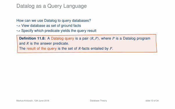
How can we use Datalog to query databases?{ View database as set of ground facts{ Specify which predicate yields the query result
Definition 11.8: A Datalog query is a pair 〈R, P〉, where P is a Datalog programand R is the answer predicate.The result of the query is the set of R-facts entailed by P.
Datalog queries distinguish “given” relations from “derived” ones:
• predicates that occur in a head of P areintensional database (IDB) predicates
• predicates that only occur in bodies areextensional database (EDB) predicates
Requirement: database relations used as EDB predicates only
Markus Krötzsch, 12th June 2018 Database Theory slide 13 of 34

Datalog as a Query Language
How can we use Datalog to query databases?{ View database as set of ground facts{ Specify which predicate yields the query result
Definition 11.8: A Datalog query is a pair 〈R, P〉, where P is a Datalog programand R is the answer predicate.The result of the query is the set of R-facts entailed by P.
Datalog queries distinguish “given” relations from “derived” ones:
• predicates that occur in a head of P areintensional database (IDB) predicates
• predicates that only occur in bodies areextensional database (EDB) predicates
Requirement: database relations used as EDB predicates only
Markus Krötzsch, 12th June 2018 Database Theory slide 13 of 34

Datalog as a Generalisation of CQs
A conjunctive query ∃y1, . . . , ym.A1 ∧ . . . ∧ A` with answer variables x1, . . . , xn can beexpressed as a Datalog query 〈Ans, P〉 where P has the single rule:
Ans(x1, . . . , xn)← A1 ∧ . . . ∧ A`
Unions of CQs can also be expressed (how?)
Intuition: Datalog generalises UCQs by adding recursion.
Markus Krötzsch, 12th June 2018 Database Theory slide 14 of 34

Datalog and UCQs
We can make the relationship of Datalog and UCQs more precise:
Definition 11.9: For a Datalog program P:
• An IDB predicate R depends on an IDB predicate S if P contains a rule withR in the head and S in the body.
• P is non-recursive if there is no cyclic dependency.
Theorem 11.10: UCQs have the same expressivity as non-recursive Datalog.
That is: a query mapping can be expressed by some UCQ if and only if it can beexpressed by a non-recursive Datalog program.
However, Datalog can be exponentially more succinct (shorter), as illustrated in anexercise.
Markus Krötzsch, 12th June 2018 Database Theory slide 15 of 34

ProofTheorem 11.10: UCQs have the same expressivity as non-recursive Datalog.
Proof: “Non-recursive Datalog can express UCQs”: Just discussed.
“UCQs can express non-recursive Datalog”
: Obtained by resolution:• Given rules ρ1 : R(s1, . . . , sn)← C1 ∧ . . . ∧ C` andρ2 : H ← B1 ∧ . . . ∧ R(t1, . . . , tn) ∧ . . . ∧ Bm
(w.l.o.g. having no variables in common with ρ1)• such that R(t1, . . . , tn) and R(s1, . . . , sn) unify with most general unifier σ,• the resolvent of ρ1 and ρ2 with respect to σ is
Hσ← B1σ ∧ . . . ∧ C1σ ∧ . . . ∧ C`σ ∧ . . . ∧ Bmσ.
Unfolding of R means to simultaneously resolve all occurrences of R in bodies of anyrule, in all possible ways. After adding all these resolvents, we can delete all rules thatcontain R in body or head (assuming that R is not the answer predicate).
Now given a non-recursive Datalog program, unfold each non-answer predicate (in anyorder). { program with only the answer predicate in heads (requires non-recursiveness).This is easy to express as UCQ (using equality to handle constants in heads). �
Markus Krötzsch, 12th June 2018 Database Theory slide 16 of 34

ProofTheorem 11.10: UCQs have the same expressivity as non-recursive Datalog.
Proof: “Non-recursive Datalog can express UCQs”: Just discussed.
“UCQs can express non-recursive Datalog”: Obtained by resolution:• Given rules ρ1 : R(s1, . . . , sn)← C1 ∧ . . . ∧ C` andρ2 : H ← B1 ∧ . . . ∧ R(t1, . . . , tn) ∧ . . . ∧ Bm
(w.l.o.g. having no variables in common with ρ1)• such that R(t1, . . . , tn) and R(s1, . . . , sn) unify with most general unifier σ,• the resolvent of ρ1 and ρ2 with respect to σ is
Hσ← B1σ ∧ . . . ∧ C1σ ∧ . . . ∧ C`σ ∧ . . . ∧ Bmσ.
Unfolding of R means to simultaneously resolve all occurrences of R in bodies of anyrule, in all possible ways. After adding all these resolvents, we can delete all rules thatcontain R in body or head (assuming that R is not the answer predicate).
Now given a non-recursive Datalog program, unfold each non-answer predicate (in anyorder). { program with only the answer predicate in heads (requires non-recursiveness).This is easy to express as UCQ (using equality to handle constants in heads). �Markus Krötzsch, 12th June 2018 Database Theory slide 16 of 34

Datalog and Domain Independence
Domain independence was considered useful for FO queries{ results should not change if domain changes
Several solutions:
• Active domain semantics: restrict to elements mentioned in database or query
• Domain-independent queries: restrict to query where domain does not matter
• Safe-range queries: decidable special case of domain independence
Our definition of Datalog uses the active domain (=Herbrand universe) to ensure domainindependence
Markus Krötzsch, 12th June 2018 Database Theory slide 17 of 34

Safe Datalog Queries
Similar to safe-range FO queries, there are also simple syntactic conditions that ensuredomain independence for Datalog:
Definition 11.11: A Datalog rule is safe if all variables in its head also occur in itsbody. A Datalog program/query is safe if all of its rules are.
Simple observations:
• safe Datalog queries are domain independent
• every Datalog query can be expressed as a safe Datalog query . . .
• . . . and un-safe queries are not much more succinct either (exercise)
Some texts require Datalog queries to be safe in generalbut in most contexts there is no real need for this
Markus Krötzsch, 12th June 2018 Database Theory slide 18 of 34

Complexity
Markus Krötzsch, 12th June 2018 Database Theory slide 19 of 34

Complexity of Datalog
How hard is answering Datalog queries?
Recall:
• Combined complexity: based on query and database
• Data complexity: based on database; query fixed
• Query complexity: based on query; database fixed
Plan:
• First show upper bounds (outline efficient algorithm)
• Then establish matching lower bounds (reduce hard problems)
Markus Krötzsch, 12th June 2018 Database Theory slide 20 of 34

A Simpler Problem: Ground Progams
Let’s start with Datalog without variables{ sets of ground rules a.k.a. propositional Horn logic program
Naive computation of T∞P :
How long does this take?
• At most |P| facts can be derived
• Algorithm terminates with i ≤ |P| + 1
• In each iteration, we check eachrule once (linear), and compare itsbody to T i
P (quadratic)
{ polynomial runtime
01 T0P := ∅
02 i := 0
03 repeat :
04 T i+1P := ∅
05 for H ← B1 ∧ . . . ∧ B` ∈ P :
06 if {B1, . . . , B`} ⊆ T iP :
07 T i+1P := T i+1
P ∪ {H}
08 i := i + 1
09 until T i−1P = T i
P
10 return T iP
Markus Krötzsch, 12th June 2018 Database Theory slide 21 of 34

Complexity of Propositional Horn Logic
Much better algorithms exist:
Theorem 11.12 (Dowling & Gallier, 1984): For a propositional Horn logic pro-gram P, the set T∞P can be computed in linear time.
Nevertheless, the problem is not trivial:
Theorem 11.13: For a propositional Horn logic program P and a proposition (orground atom) A, deciding if A ∈ T∞P is a P-complete problem.
Remark:all P problems can be reduced to propositional Horn logic entailmentyet not all problems in P (or even in NL) can be solved in linear time!
Markus Krötzsch, 12th June 2018 Database Theory slide 22 of 34

Datalog Complexity: Upper Bounds
A straightforward approach:
(1) Compute the grounding ground(P) of P w.r.t. the database I
(2) Compute T∞ground(P)
Complexity estimation:
• The number of constants N for grounding is linear in P and I
• A rule with m distinct variables has Nm ground instances• Step (1) creates at most |P| · NM ground rules, where M is the maximal number of
variables in any rule in P– ground(P) is polynomial in the size of I– ground(P) is exponential in P
• Step (2) can be executed in linear time in the size of ground(P)
Summing up: the algorithm runs in P data complexity and in ExpTime query andcombined complexity
Markus Krötzsch, 12th June 2018 Database Theory slide 23 of 34

Datalog Complexity
These upper bounds are tight:
Theorem 11.14: Datalog query answering is:
• ExpTime-complete for combined complexity
• ExpTime-complete for query complexity
• P-complete for data complexity
It remains to show the lower bounds.
Markus Krötzsch, 12th June 2018 Database Theory slide 24 of 34

P-Hardness of Data Complexity
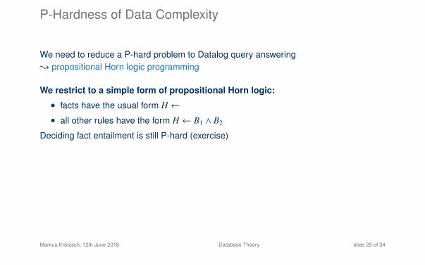
We need to reduce a P-hard problem to Datalog query answering{ propositional Horn logic programming
We restrict to a simple form of propositional Horn logic:
• facts have the usual form H ←
• all other rules have the form H ← B1 ∧ B2
Deciding fact entailment is still P-hard (exercise)
We can store such programs in a database:
• For each fact H ←, the database has a tuple Fact(H)
• For each rule H ← B1 ∧ B2,the database has a tuple Rule(H, B1, B2)
Markus Krötzsch, 12th June 2018 Database Theory slide 25 of 34
P-Hardness of Data Complexity
We need to reduce a P-hard problem to Datalog query answering{ propositional Horn logic programming
We restrict to a simple form of propositional Horn logic:
• facts have the usual form H ←
• all other rules have the form H ← B1 ∧ B2
Deciding fact entailment is still P-hard (exercise)
We can store such programs in a database:
• For each fact H ←, the database has a tuple Fact(H)
• For each rule H ← B1 ∧ B2,the database has a tuple Rule(H, B1, B2)
Markus Krötzsch, 12th June 2018 Database Theory slide 25 of 34

P-Hardness of Data Complexity (2)
The following Datalog program acts as an interpreter for propositional Horn logicprograms:
True(x)← Fact(x)
True(x)← Rule(x, y, z) ∧ True(y) ∧ True(z)
Easy observations:
• True(A) is derived if and only if A is a consequence of the original propositionalprogram
• The encoding of propositional programs as databases can be computed inlogarithmic space
• The Datalog program is the same for all propositional programs
{ Datalog query answering is P-hard for data complexity
Markus Krötzsch, 12th June 2018 Database Theory slide 26 of 34

ExpTime-Hardness of Query Complexity
A direct proof:Encode the computation of a deterministic Turing machine for up to exponentially manysteps
Recall that ExpTime =⋃
k≥1 Time(2nk)
• in our case, n = N is the number of database constants
• k is some constant
{ we need to simulate up to 2Nksteps (and tape cells)
Main ingredients of the encoding:
• stateq(X): the TM is in state q after X steps
• head(X, Y): the TM head is at tape position Y after X steps
• symbolσ(X, Y): the tape cell at position Y holds symbol σ after X steps
{ How to encode 2Nktime points X and tape positions Y?
Markus Krötzsch, 12th June 2018 Database Theory slide 27 of 34

Preparing for a Long Computation
We need to encode 2Nktime points and tape positions
{ use binary numbers with Nk digits
So X and Y in atoms like head(X, Y) are really lists of variables X = x1, . . . , xNk andY = y1, . . . , yNk , and the arity of head is 2 · Nk.
TODO: define predicates that capture the order of Nk-digit binary numbers
For each number i ∈ {1, . . . , Nk}, we use predicates:
• succi(X, Y): X + 1 = Y, where X and Y are i-digit numbers
• firsti(X): X is the i-digit encoding of 0
• lasti(X): X is the i-digit encoding of 2i − 1
Finally, we can define the actual order for i = Nk
• ≤i (X, Y): X ≤ Y, where X and Y are i-digit numbers
Markus Krötzsch, 12th June 2018 Database Theory slide 28 of 34

Defining a Long Chain
We can define succi(X, Y), firsti(X), and lasti(X) as follows:
succ1(0, 1) first1(0) last1(1)
succi+1(0, X, 0, Y)← succi(X, Y)
succi+1(1, X, 1, Y)← succi(X, Y)
succi+1(0, X, 1, Y)← lasti(X) ∧ firsti(Y)
for X = x1, . . . , xi
and Y = y1, . . . , yi
lists of i variablesfirsti+1(0, X)← firsti(X)
lasti+1(1, X)← lasti(X)
Now for M = Nk , we define ≤M(X, Y) as the reflexive, transitive closure of succM(X, Y):
≤M(X, X)←
≤M(X, Z)← ≤M(X, Y) ∧ succM(Y, Z)
Markus Krötzsch, 12th June 2018 Database Theory slide 29 of 34
Initialising the Computation
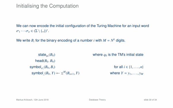
We can now encode the initial configuration of the Turing Machine for an input wordσ1 · · ·σn ∈ (Σ \ {�})∗.
We write Bi for the binary encoding of a number i with M = Nk digits.
stateq0 (B0) where q0 is the TM’s initial state
head(B0, B0)
symbolσi(B0, Bi) for all i ∈ {1, . . . , n}
symbol�(B0, Y)← ≤M(Bn+1, Y) where Y = y1, . . . , yM
Markus Krötzsch, 12th June 2018 Database Theory slide 30 of 34

TM Transition and Acceptance RulesFor each transition 〈q,σ, q′,σ′, d〉 ∈ ∆, we add rules:
symbolσ′ (X′, Y)← succM(X, X′) ∧ head(X, Y) ∧ symbolσ(X, Y) ∧ stateq(X)
stateq′ (X′)← succM(X, X′) ∧ head(X, Y) ∧ symbolσ(X, Y) ∧ stateq(X)
Similar rules are used for inferring the new head position (depending on d)
Further rules ensure the preservation of unaltered tape cells:
symbolσ(X′, Y)← succM(X, X′) ∧ symbolσ(X, Y) ∧
head(X, Z) ∧ succM(Z, Z′) ∧ ≤M(Z′, Y)
symbolσ(X′, Y)← succM(X, X′) ∧ symbolσ(X, Y) ∧
head(X, Z) ∧ succM(Z′, Z) ∧ ≤M(Y, Z′)
The TM accepts if it ever reaches the accepting state qacc:
accept()← stateqacc (X)
Markus Krötzsch, 12th June 2018 Database Theory slide 31 of 34

Hardness Results
Lemma 11.15: A deterministic TM accepts an input in Time(2nk) if and only if the
Datalog program defined above entails the fact accept().
We obtain ExpTime-hardness of Datalog query answering:
• The decision problem of any language in ExpTime can be solved by a deterministicTM in Time(2nk
) for some constant k
• In particular, there are ExpTime-hard languages L with suitable deterministic TMM and constant k
• For any input word w, we can reduce acceptance of w byM in Time(2nk) to
entailment of accept() by a Datalog program P(w,M, k)
• P(w,M, k) is polynomial in k and the size ofM and w(in fact, it can be constructed in logarithmic space)
Markus Krötzsch, 12th June 2018 Database Theory slide 32 of 34

ExpTime-Hardness: Notes
Some further remarks on our construction:
• The constructed program does not use EDB predicates{ database can be empty
• Therefore, hardness extends to query complexity
• Using a fixed (very small) database, we could have avoided the use of constants
• We used IDB predicates of unbounded arity{ they are essential for the claimed hardness
Markus Krötzsch, 12th June 2018 Database Theory slide 33 of 34

Summary and Outlook
Datalog can overcome some of the limitations of first-order queries
Non-recursive Datalog can express UCQs
Datalog is more complex than FO query answering:
• ExpTime-complete for query and combined complexity
• P-complete for data complexity
Open questions:
• Expressivity of Datalog
• Query containment for Datalog
• Implementation techniques for Datalog
Markus Krötzsch, 12th June 2018 Database Theory slide 34 of 34


![Datalog: Bag Semantics via Set Semantics - arXiv · Datalog±share these properties: for instance, guarded [8], sticky and weakly-sticky [11] Datalog ± only allow restricted forms](https://static.fdocuments.in/doc/165x107/5e7e36effe39a8678f12fd4f/datalog-bag-semantics-via-set-semantics-arxiv-datalogshare-these-properties.jpg)