Database System Concepts 5 th Ed. ©Silberschatz, Korth and Sudarshan Chapter 14: Query...

Database System Concepts 5th Ed.

©Silberschatz, Korth and Sudarshan

Chapter 14: Query OptimizationChapter 14: Query Optimization

©Silberschatz, Korth and Sudarshan14.2Database System Concepts - 5th Edition, Oct 5, 2006.

Query OptimizationQuery Optimization

Process of selecting the most efficient query evaluation plan (QEP) from among the many strategies usually possible for processing a given query, especially if the query is complex.

This is expected out of the system and not the users.

Three step process:

1. Generate expressions that are logically equivalent to given expression

2. Estimate the cost of each QEP

3. Annotating the resultant expressions in alternative ways to generate QEP

While (1) and (3) are interleaved in the optimizer, (2) is done in the background by collecting statistical information about relations (such as sizes, index depth, etc.) to make a good estimate of the cost of a QEP.


IntroductionIntroduction

Alternative ways of evaluating a given query

Equivalent expressions

Different algorithms for each operation


Introduction (Cont.)Introduction (Cont.)

Query: Find the names of all customers who have an account at some branch located in Brooklyn.customer_name(branch_city = “Brooklyn”

(branch (account depositor)))

Transformation using rule 7a. customer_name

((branch_city =“Brooklyn” (branch)) (account depositor))

Performing the selection as early as possible reduces the size of the relation to be joined.



An evaluation plan defines exactly what algorithm is used for each operation, and how the execution of the operations is coordinated.



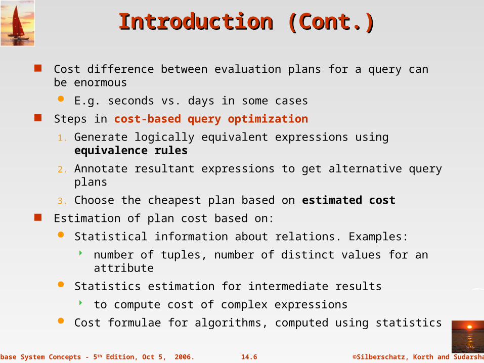
Cost difference between evaluation plans for a query can be enormous

E.g. seconds vs. days in some cases

Steps in cost-based query optimization

1. Generate logically equivalent expressions using equivalence rules

2. Annotate resultant expressions to get alternative query plans

3. Choose the cheapest plan based on estimated cost

Estimation of plan cost based on:

Statistical information about relations. Examples:

number of tuples, number of distinct values for an attribute

Statistics estimation for intermediate results

to compute cost of complex expressions

Cost formulae for algorithms, computed using statistics



Generating Equivalent ExpressionsGenerating Equivalent Expressions


Transformation of Relational ExpressionsTransformation of Relational Expressions

Two relational algebra expressions are said to be equivalent if the two expressions generate the same set of tuples on every legal database instance

Note: order of tuples is irrelevant

In SQL, inputs and outputs are multisets of tuples

Two expressions in the multiset version of the relational algebra are said to be equivalent if the two expressions generate the same multiset of tuples on every legal database instance.

An equivalence rule says that expressions of two forms are equivalent

Can replace expression of first form by second, or vice versa

Refer textbook for 12 rules (pgs 571 through 574)


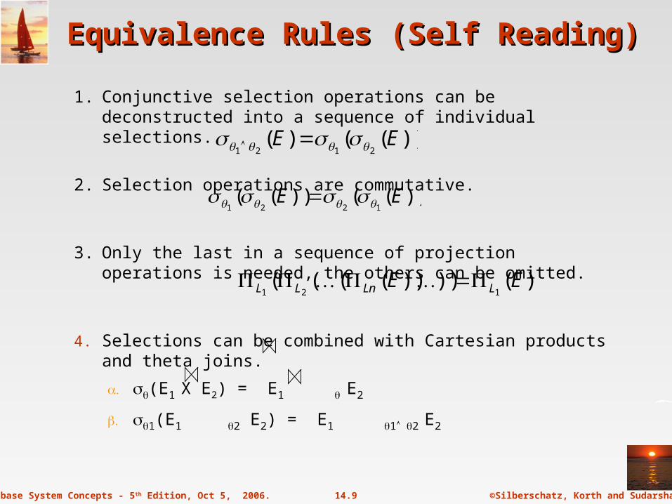
Equivalence Rules (Self Reading)Equivalence Rules (Self Reading)

1. Conjunctive selection operations can be deconstructed into a sequence of individual selections.

2. Selection operations are commutative.

3. Only the last in a sequence of projection operations is needed, the others can be omitted.

4. Selections can be combined with Cartesian products and theta joins.

a. (E1 X E2) = E1 E2

b. 1(E1 2 E2) = E1 1 2 E2

))(())((1221EE

))(()(2121EE

)())))((((121EE LLnLL


Equivalence Rules (Cont.)Equivalence Rules (Cont.)

5. Theta-join operations (and natural joins) are commutative.E1 E2 = E2 E1

6. (a) Natural join operations are associative:

(E1 E2) E3 = E1 (E2 E3)

(b) Theta joins are associative in the following manner:

(E1 1 E2) 2 3 E3 = E1 1 3 (E2 2 E3) where 2 involves attributes from only E2 and E3.


Pictorial Depiction of Equivalence RulesPictorial Depiction of Equivalence Rules



7. The selection operation distributes over the theta join operation under the following two conditions:(a) When all the attributes in 0 involve only the attributes of one of the expressions (E1) being joined.

0E1 E2) = (0(E1)) E2

(b) When 1 involves only the attributes of E1 and 2 involves only the attributes of E2.

1 E1 E2) = (1(E1)) ( (E2))



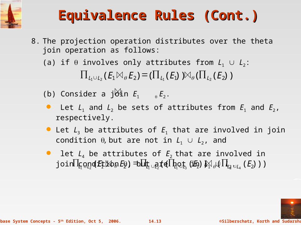
8. The projection operation distributes over the theta join operation as follows:

(a) if involves only attributes from L1 L2:

(b) Consider a join E1 E2.

Let L1 and L2 be sets of attributes from E1 and E2, respectively.

Let L3 be attributes of E1 that are involved in join condition , but are not in L1 L2, and

let L4 be attributes of E2 that are involved in join condition , but are not in L1 L2.

))(())(()( 2121 2121EEEE LLLL

)))(())((()( 2121 42312121EEEE LLLLLLLL



9. The set operations union and intersection are commutative E1 E2 = E2 E1 E1 E2 = E2 E1

(set difference is not commutative).

10. Set union and intersection are associative.

(E1 E2) E3 = E1 (E2 E3)

(E1 E2) E3 = E1 (E2 E3)

11. The selection operation distributes over , and –.

(E1 – E2) = (E1) – (E2)

and similarly for and in place of –

Also: (E1 – E2) = (E1) – E2

and similarly for in place of –, but not for

12. The projection operation distributes over union

L(E1 E2) = (L(E1)) (L(E2))


Join Ordering ExampleJoin Ordering Example

Good order is important for reducing the size of temporary results.

Natural Join is commutative.

For all relations r1, r2, and r3,

(r1 r2) r3 = r1 (r2 r3 )

(Join Associativity)

If r2 r3 is quite large and r1 r2 is small, we choose

(r1 r2) r3

so that we compute and store a smaller temporary relation.


Join Ordering Example (Cont.)Join Ordering Example (Cont.)

Consider the expression

customer_name ((branch_city = “Brooklyn” (branch)) (account depositor))

Could compute account depositor first, and join result with branch_city = “Brooklyn” (branch)

but account depositor is likely to be a large relation.

Only a small fraction of the bank’s customers are likely to have accounts in branches located in Brooklyn

it is better to compute

branch_city = “Brooklyn” (branch) account

first.


Choice of Evaluation PlansChoice of Evaluation Plans

Must consider the interaction of evaluation techniques when choosing evaluation plans

choosing the cheapest algorithm for each operation independently may not yield best overall algorithm. E.g.

merge-join may be costlier than hash-join, but may provide a sorted output which reduces the cost for an outer level aggregation.

nested-loop join may provide opportunity for pipelining

Practical query optimizers incorporate elements of the following two broad approaches:

1. Search all the plans and choose the best plan in a cost-based fashion.

2. Uses heuristics to choose a plan.


Left Deep Join TreesLeft Deep Join Trees

In left-deep join trees, the right-hand-side input for each join is a relation, not the result of an intermediate join.


Heuristic OptimizationHeuristic Optimization

Cost-based optimization is expensive

Systems may use heuristics to reduce the number of choices that must be made in a cost-based fashion.

Heuristic optimization transforms the query-tree by using a set of rules that typically (but not in all cases) improve execution performance:

Perform selection early (reduces the number of tuples)

Perform projection early (reduces the number of attributes)

Perform most restrictive selection and join operations (i.e. with smallest result size) before other similar operations.

Some systems use only heuristics, others combine heuristics with partial cost-based optimization.



Statistics for Cost EstimationStatistics for Cost Estimation(Self Reading)(Self Reading)


Statistical Information for Cost EstimationStatistical Information for Cost Estimation

nr: number of tuples in a relation r.

br: number of blocks containing tuples of r.

lr: size of a tuple of r.

fr: blocking factor of r — i.e., the number of tuples of r that fit into one block.

V(A, r): number of distinct values that appear in r for attribute A; same as the size of A(r).

If tuples of r are stored together physically in a file, then:

rfrn

rb


HistogramsHistograms

Histogram on attribute age of relation person

Equi-width histograms

Equi-depth histograms


Selection Size EstimationSelection Size Estimation

A=v(r)

nr / V(A,r) : number of records that will satisfy the selection

Equality condition on a key attribute: size estimate = 1

AV(r) (case of A V(r) is symmetric)

Let c denote the estimated number of tuples satisfying the condition.

If min(A,r) and max(A,r) are available in catalog

c = 0 if v < min(A,r)

c =

If histograms available, can refine above estimate

In absence of statistical information c is assumed to be nr / 2.

),min(),max(

),min(.

rArA

rAvnr


Size Estimation of Complex SelectionsSize Estimation of Complex Selections

The selectivity of a condition i is the probability that a tuple in the relation r

satisfies i .

If si is the number of satisfying tuples in r, the selectivity of i is given by si /nr.

Conjunction: 1 2. . . n (r). Assuming indepdence, estimate of

tuples in the result is:

Disjunction:1 2 . . . n (r). Estimated number of tuples:

Negation: (r). Estimated number of tuples:

nr – size((r))

nr

nr n

sssn

. . . 21

)1(...)1()1(1 21

r

n

rrr n

s

n

s

n

sn


Join Operation: Running ExampleJoin Operation: Running Example

Running example: depositor customer

Catalog information for join examples:

ncustomer = 10,000.

fcustomer = 25, which implies that

bcustomer =10000/25 = 400.

ndepositor = 5000.

fdepositor = 50, which implies that

bdepositor = 5000/50 = 100.

V(customer_name, depositor) = 2500, which implies that , on average, each customer has two accounts. Also assume that customer_name in depositor is a foreign key

on customer. V(customer_name, customer) = 10000 (primary key!)


Estimation of the Size of JoinsEstimation of the Size of Joins

The Cartesian product r x s contains nr .ns tuples; each tuple occupies sr + ss bytes.

If R S = , then r s is the same as r x s.

If R S is a key for R, then a tuple of s will join with at most one tuple from r

therefore, the number of tuples in r s is no greater than the number of tuples in s.

If R S in S is a foreign key in S referencing R, then the number of tuples in r s is exactly the same as the number of tuples in s.

The case for R S being a foreign key referencing S is symmetric.

In the example query depositor customer, customer_name in depositor is a foreign key of customer

hence, the result has exactly ndepositor tuples, which is 5000


Estimation of the Size of Joins (Cont.)Estimation of the Size of Joins (Cont.)

If R S = {A} is not a key for R or S.If we assume that every tuple t in R produces tuples in R S, the number of tuples in R S is estimated to be:

If the reverse is true, the estimate obtained will be:

The lower of these two estimates is probably the more accurate one.

Can improve on above if histograms are available

Use formula similar to above, for each cell of histograms on the two relations

),( sAVnn sr

),( rAVnn sr


Estimation of the Size of Joins (Cont.)Estimation of the Size of Joins (Cont.)

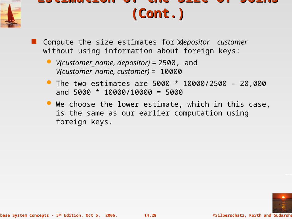
Compute the size estimates for depositor customer without using information about foreign keys:

V(customer_name, depositor) = 2500, andV(customer_name, customer) = 10000

The two estimates are 5000 * 10000/2500 - 20,000 and 5000 * 10000/10000 = 5000

We choose the lower estimate, which in this case, is the same as our earlier computation using foreign keys.


Size Estimation for Other OperationsSize Estimation for Other Operations

Projection: estimated size of A(r) = V(A,r)

Aggregation : estimated size of AgF(r) = V(A,r)

Set operations

For unions/intersections of selections on the same relation: rewrite and use size estimate for selections

E.g. 1 (r) 2 (r) can be rewritten as 1 2 (r)

For operations on different relations:

estimated size of r s = size of r + size of s.

estimated size of r s = minimum size of r and size of s.

estimated size of r – s = r.

All the three estimates may be quite inaccurate, but provide upper bounds on the sizes.


Size Estimation (Cont.)Size Estimation (Cont.)

Outer join:

Estimated size of r s = size of r s + size of r

Case of right outer join is symmetric

Estimated size of r s = size of r s + size of r + size of s


Estimation of Number of Distinct ValuesEstimation of Number of Distinct Values

Selections: (r)

If forces A to take a specified value: V(A, (r)) = 1.

e.g., A = 3

If forces A to take on one of a specified set of values: V(A, (r)) = number of specified values.

(e.g., (A = 1 V A = 3 V A = 4 )),

If the selection condition is of the form A op restimated V(A, (r)) = V(A.r) * s

where s is the selectivity of the selection.

In all the other cases: use approximate estimate of min(V(A,r), n (r) )

More accurate estimate can be got using probability theory, but this one works fine generally


Estimation of Distinct Values (Cont.)Estimation of Distinct Values (Cont.)

Joins: r s

If all attributes in A are from r estimated V(A, r s) = min (V(A,r), n r s)

If A contains attributes A1 from r and A2 from s, then estimated V(A,r s) =

min(V(A1,r)*V(A2 – A1,s), V(A1 – A2,r)*V(A2,s), nr s)

More accurate estimate can be got using probability theory, but this one works fine generally


Estimation of Distinct Values (Cont.)Estimation of Distinct Values (Cont.)

Estimation of distinct values are straightforward for projections.

They are the same in A (r) as in r.

The same holds for grouping attributes of aggregation.

For aggregated values

For min(A) and max(A), the number of distinct values can be estimated as min(V(A,r), V(G,r)) where G denotes grouping attributes

For other aggregates, assume all values are distinct, and use V(G,r)



Additional Optimization TechniquesAdditional Optimization Techniques (Self Reading) (Self Reading)

Nested Subqueries

Materialized Views


Optimizing Nested Subqueries**Optimizing Nested Subqueries**

Nested query example:select customer_namefrom borrowerwhere exists (select *

from depositor where depositor.customer_name =

borrower.customer_name)

SQL conceptually treats nested subqueries in the where clause as functions that take parameters and return a single value or set of values

Parameters are variables from outer level query that are used in the nested subquery; such variables are called correlation variables

Conceptually, nested subquery is executed once for each tuple in the cross-product generated by the outer level from clause

Such evaluation is called correlated evaluation

Note: other conditions in where clause may be used to compute a join (instead of a cross-product) before executing the nested subquery


Optimizing Nested Subqueries (Cont.)Optimizing Nested Subqueries (Cont.)

Correlated evaluation may be quite inefficient since

a large number of calls may be made to the nested query

there may be unnecessary random I/O as a result

SQL optimizers attempt to transform nested subqueries to joins where possible, enabling use of efficient join techniques

E.g.: earlier nested query can be rewritten as select customer_namefrom borrower, depositorwhere depositor.customer_name = borrower.customer_name

Note: the two queries generate different numbers of duplicates (why?)

Borrower can have duplicate customer-names

Can be modified to handle duplicates correctly as we will see

In general, it is not possible/straightforward to move the entire nested subquery from clause into the outer level query from clause

A temporary relation is created instead, and used in body of outer level query



In general, SQL queries of the form below can be rewritten as shown Rewrite: select …

from L1

where P1 and exists (select * from L2

where P2)

To: create table t1 as select distinct V from L2

where P21

select … from L1, t1 where P1 and P2

2

P21 contains predicates in P2 that do not involve any correlation

variables P2

2 reintroduces predicates involving correlation variables, with relations renamed appropriately

V contains all attributes used in predicates with correlation variables



In our example, the original nested query would be transformed to create table t1 as select distinct customer_name from depositor select customer_name from borrower, t1

where t1.customer_name = borrower.customer_name

The process of replacing a nested query by a query with a join (possibly with a temporary relation) is called decorrelation.

Decorrelation is more complicated when

the nested subquery uses aggregation, or

when the result of the nested subquery is used to test for equality, or

when the condition linking the nested subquery to the other query is not exists,

and so on.


Materialized Views**Materialized Views**

A materialized view is a view whose contents are computed and stored.

Consider the viewcreate view branch_total_loan(branch_name, total_loan) asselect branch_name, sum(amount)from loangroup by branch_name

Materializing the above view would be very useful if the total loan amount is required frequently

Saves the effort of finding multiple tuples and adding up their amounts


Materialized View MaintenanceMaterialized View Maintenance

The task of keeping a materialized view up-to-date with the underlying data is known as materialized view maintenance

Materialized views can be maintained by recomputation on every update

A better option is to use incremental view maintenance

Changes to database relations are used to compute changes to the materialized view, which is then updated

View maintenance can be done by

Manually defining triggers on insert, delete, and update of each relation in the view definition

Manually written code to update the view whenever database relations are updated

Periodic recomputation (e.g. nightly)

Above methods are directly supported by many database systems

Avoids manual effort/correctness issues


Incremental View MaintenanceIncremental View Maintenance

The changes (inserts and deletes) to a relation or expressions are referred to as its differential

Set of tuples inserted to and deleted from r are denoted ir and dr

To simplify our description, we only consider inserts and deletes

We replace updates to a tuple by deletion of the tuple followed by insertion of the update tuple

We describe how to compute the change to the result of each relational operation, given changes to its inputs

We then outline how to handle relational algebra expressions


Join OperationJoin Operation

Consider the materialized view v = r s and an update to r

Let rold and rnew denote the old and new states of relation r

Consider the case of an insert to r:

We can write rnew s as (rold ir) s

And rewrite the above to (rold s) (ir s)

But (rold s) is simply the old value of the materialized view, so the

incremental change to the view is just ir s

Thus, for inserts vnew = vold (ir s)

Similarly for deletes vnew = vold – (dr s)

A, 1B, 2

1, p2, r2, s

A, 1, pB, 2, rB, 2, s

C,2C, 2, rC, 2, s


Selection and Projection OperationsSelection and Projection Operations

Selection: Consider a view v = (r).

vnew = vold (ir)

vnew = vold - (dr) Projection is a more difficult operation

R = (A,B), and r(R) = { (a,2), (a,3)} A(r) has a single tuple (a). If we delete the tuple (a,2) from r, we should not delete the tuple (a)

from A(r), but if we then delete (a,3) as well, we should delete the tuple

For each tuple in a projection A(r) , we will keep a count of how many times it was derived On insert of a tuple to r, if the resultant tuple is already in A(r) we

increment its count, else we add a new tuple with count = 1 On delete of a tuple from r, we decrement the count of the

corresponding tuple in A(r)

if the count becomes 0, we delete the tuple from A(r)


Aggregation OperationsAggregation Operations

count : v = Agcount(B)(r).

When a set of tuples ir is inserted

For each tuple r in ir, if the corresponding group is already present in v,

we increment its count, else we add a new tuple with count = 1

When a set of tuples dr is deleted

for each tuple t in ir.we look for the group t.A in v, and subtract 1 from

the count for the group.

– If the count becomes 0, we delete from v the tuple for the group t.A

sum: v = Agsum (B)(r)

We maintain the sum in a manner similar to count, except we add/subtract the B value instead of adding/subtracting 1 for the count

Additionally we maintain the count in order to detect groups with no tuples. Such groups are deleted from v

Cannot simply test for sum = 0 (why?)

To handle the case of avg, we maintain the sum and count aggregate values separately, and divide at the end


Aggregate Operations (Cont.)Aggregate Operations (Cont.)

min, max: v = Agmin (B) (r).

Handling insertions on r is straightforward.

Maintaining the aggregate values min and max on deletions may be more expensive. We have to look at the other tuples of r that are in the same group to find the new minimum


Other OperationsOther Operations

Set intersection: v = r s

when a tuple is inserted in r we check if it is present in s, and if so we add it to v.

If the tuple is deleted from r, we delete it from the intersection if it is present.

Updates to s are symmetric

The other set operations, union and set difference are handled in a similar fashion.

Outer joins are handled in much the same way as joins but with some extra work

we leave details to you.


Handling ExpressionsHandling Expressions

To handle an entire expression, we derive expressions for computing the incremental change to the result of each sub-expressions, starting from the smallest sub-expressions.

E.g. consider E1 E2 where each of E1 and E2 may be a complex expression

Suppose the set of tuples to be inserted into E1 is given by D1

Computed earlier, since smaller sub-expressions are handled first

Then the set of tuples to be inserted into E1 E2 is given by D1 E2

This is just the usual way of maintaining joins


Query Optimization and Materialized ViewsQuery Optimization and Materialized Views

Rewriting queries to use materialized views:

A materialized view v = r s is available

A user submits a query r s t

We can rewrite the query as v t

Whether to do so depends on cost estimates for the two alternative

Replacing a use of a materialized view by the view definition:

A materialized view v = r s is available, but without any index on it

User submits a query A=10(v).

Suppose also that s has an index on the common attribute B, and r has an index on attribute A.

The best plan for this query may be to replace v by r s, which can lead to the query plan A=10(r) s

Query optimizer should be extended to consider all above alternatives and choose the best overall plan


Materialized View SelectionMaterialized View Selection

Materialized view selection: “What is the best set of views to materialize?”.

Index selection: “what is the best set of indices to create”

closely related, to materialized view selection but simpler

Materialized view selection and index selection based on typical system workload (queries and updates)

Typical goal: minimize time to execute workload , subject to constraints on space and time taken for some critical queries/updates

One of the steps in database tuning

more on tuning in later chapters

Commercial database systems provide tools (called “tuning assistants” or “wizards”) to help the database administrator choose what indices and materialized views to create



Extra Slides:Extra Slides:Additional Optimization TechniquesAdditional Optimization Techniques

(Self Reading) (Self Reading)

(see bibliographic notes)


Top-K QueriesTop-K Queries

Top-K queries

select * from r, swhere r.B = s.Border by r.A ascendinglimit 10

Alternative 1: Indexed nested loops join with r as outer

Alternative 2: estimate highest r.A value in result and add selection (and r.A <= H) to where clause

If < 10 results, retry with larger H


Optimization of UpdatesOptimization of Updates

Halloween problem

update R set A = 5 * A where A > 10

If index on A is used to find tuples satisfying A > 10, and tuples updated immediately, same tuple may be found (and updated) multiple times

Solution 1: Always defer updates

collect the updates (old and new values of tuples) and update relation and indices in second pass

Drawback: extra overhead even if e.g. update is only on R.B, not on attributes in selection condition

Solution 2: Defer only if required

Perform immediate update if update does not affect attributes in where clause, and deferred updates otherwise.


Parametric Query OptimizationParametric Query Optimization

Example select * from r natural join swhere r.a < $1

value of parameter $1 not known at compile time known only at run time

different plans may be optimal for different values of $1 Solution 1: optimize at run time, each time query is submitted

can be expensive Solution 2: Parametric Query Optimization:

optimizer generates a set of plans, optimal for different values of $1 Set of optimal plans usually small for 1 to 3 parameters Key issue: how to do find set of optimal plans efficiently

best one from this set is chosen at run time when $1 is known Solution 3: Query Plan Caching

If optimizer decides that same plan is likely to be optimal for all parameter values, it caches plan and reuses it, else reoptimize each time

Implemented in many database systems


Join MinimizationJoin Minimization

Join minimization

select r.A, r.B from r, swhere r.B = s.B

Check if join with s is redundant, drop it

E.g. join condition is on foreign key from r to s, no selection on s

Other sufficient conditions possibleselect r.A, s1.B from r, s as s1, s as s2

where r.B=s1.B and r.B = s2.B and s1.A < 20 and s2.A < 10

join with s2 is redundant and can be dropped (along with selection on s2)

Lots of research in this area since 70s/80s!


Multiquery OptimizationMultiquery Optimization

Example

Q1: select * from (r natural join t) natural join s

Q2: select * from (r natural join u) natural join s Both queries share common subexpression (r natural join s) May be useful to compute (r natural join s) once and use it in both queries

But this may be more expensive in some situations

– e.g. (r natural join s) may be expensive, plans as shown in queries may be cheaper

Multiquery optimization: find best overall plan for a set of queries, expoiting sharing of common subexpressions between queries where it is useful

Simple heuristic used in some database systems: optimize each query separately detect and exploiting common subexpressions in the individual optimal

query plans May not always give best plan, but is cheap to implement

Set of materialized views may share common subexpressions As a result, view maintenance plans may share subexpressions Multiquery optimization can be useful in such situations



End of ChapterEnd of Chapter

Database System Concepts 5 th Ed. ©Silberschatz, Korth and Sudarshan Chapter 14: Query...

Documents

Transcript of Database System Concepts 5 th Ed. ©Silberschatz, Korth and Sudarshan Chapter 14: Query...