Data Worth of the Hydraulic Conductivity Measurements: Slug Test and Pumping Test

Willy Zawadzki

B.Sc., University of British Columbia, 1994

A THESIS SUBMITTED IN PARTIAL FULFILLMENT OF T H E REQUIREMENTS

FOR T H E DEGREE OF MASTERS OF SCIENCE

IN

T H E F A C U L T Y OF G R A D U A T E STUDIES

DEPARTMENT OF E A R T H AND O C E A N SCIENCES

We accept this thesis as conforming to the required standard:

THE UNIVERSITY OF BRITISH COLUMBIA

June 1996

© Willy Zawadzki, 1996

In presenting this thesis in partial fulfilment of the requirements for an advanced

degree at the University of British Colurhbia, I agree that the Library shall make it

freely available for reference and study. I further agree that permission for extensive

copying of this thesis for scholarly purposes may be granted by the head of my

department or by his or her representatives. It is understood that copying or

publication of this thesis for financial gain shall not be allowed without my written

permission.

Department of 6tyr UH(j QflBQfl ^CJOMC^

The University of British Columbia Vancouver, Canada

Date QCT.il,

DE-6 (2/88)

A B S T R A C T

The high cost of groundwater remediation is directly related to hydrogeological uncertainty. Of several

parameters responsible for that uncertainty, hydraulic conductivity (K) is the most important, and at the

same time the most difficult to estimate. K can be measured in the lab or field using permeameter tests,

piezocone tests, slug tests and pumping tests. However, the hydraulic conductivities measured with these

tests are not directly comparable because they characterize different volumes of the subsurface. In practice,

one would like to know which method can be used to solve the engineering problem at hand most cost-

effectively. For example, is it cheaper from the risk-cost-benefit standpoint to take small-scale

measurements with slug tests, or larger-scale measurements using pumping tests? Which method will

provide greatest reduction in the uncertainty of the hydraulic conductivity field?

I focus on the value of the two most commonly used field techniques, the slug test and pumping test, and

address the problem using an empirical/numerical approach. First I examine the averaging properties of

the pumping test using sensitivity analysis. The pumping-test averaging volume has an elliptical shape,

and its size is proportional to the test duration and to the distance between the pumping well and the

observation well. The averaging exhibits characteristic zonation, with zones behind and in-between the

wells having the strongest impact on the pumping-test scale K. Additionally, the analysis shows the inter-

well zone influences the pumping-test K for tests of all duration. While the above mentioned properties of

a pumping-test averaging volume disintegrate with increasing heterogeneity, some characteristic features

can still be distinguished, even for strongly heterogeneous K fields.

Next I develop a data-worth methodology applicable to measurements taken at different scales. The

method relies upon the representation of larger-scale measured parameters as spatially-averaged smaller-

scale parameters. It combines a decision model, a hydraulic conductivity uncertainty model, and

groundwater flow model employed in a Monte Carlo mode. I apply the data-worth methodology to a

generic contamination scenario, where a decision maker is faced with contamination of a 2-D aquifer. The

results show that a single pumping-test measurement has higher worth than a single slug-test

ii

measurement, and that the worth of a pumping-test measurement increases with increasing distance

between the observation well and the pumping well. The worth of two slug-test measurements is

comparable with the worth of a small scale pumping-test measurement, however the large scale pumping-

test measurement still proves to be more valuable. The higher data-worth of pumping test suggests that, on

sites with configuration similar to the generic scenario, measurements with large averaging volume

provide greater reduction in risk, and have greater impact on the decision making process.

iii

T A B L E OF CONTENTS

A B S T R A C T ii

T A B L E O F C O N T E N T S . . . iv

L I S T O F T A B L E S ..vi

L I S T O F F I G U R E S vii

A C K N O W L E G M E N T S viii

1. I N T R O D U C T I O N 1

2. A V E R A G I N G V O L U M E S O F S L U G T E S T S A N D P U M P I N G T E S T S 4

2.1 I N T R O D U C T I O N 4

2.2 M E T H O D S F O R E S T I M A T I N G A V E R A G I N G V O L U M E S 5

2.3 S L U G T E S T . . . . 6

2.3.1 T E S T I N G P R O C E D U R E S A N D M E T H O D S FOR D A T A INTERPRETATION 6

2.3.2 S L U G T E S T A V E R A G I N G V O L U M E 9

2.4 P U M P I N G T E S T 10

2.4.1 T E S T I N G P R O C E D U R E A N D M E T H O D S FOR D A T A INTERPRETATION 11

2.4.2 EXISTING ESTIMATES OF PUMPING TEST A V E R A G I N G V O L U M E 13

2.4.3 P U M P I N G T E S T V O L U M E VIA SENsrnvrrY ANALYSIS 14

2.5 C O N C L U S I O N 24

3. M E T H O D O L O G Y F O R E S T A B L I S H I N G D A T A W O R T H 26

3.1 I N T R O D U C T I O N 26

3.2 D E C I S I O N A N A L Y S I S 26

3.3 G E N E R I C C O N T A M I N A T I O N S C E N A R I O 28

3.4 F O U R S T E P M E T H O D O L O G Y .29

3.4.1 U N C E R T A I N T Y M O D E L FOR H Y D R A U L I C CONDUCTIVITY (STEP 1) 30

iv

3.4.2 PRIOR ANALYSIS (STEP 2) 32

3.4.3 E X H A U S T I V E U P D A T I N G 35

3.4.4 PREPOSTERIOR ANALYSIS (STEP 3) I 37

3.4.5 D A T A W O R T H (STEP 4) 38

4. W O R T H O F S L U G T E S T A N D P U M P I N G T E S T 39

4.1 I N T R O D U C T I O N 39

4.2 D A T A W O R T H O F A S I N G L E S L U G T E S T V E R S U S A S I N G L E P U M P I N G T E S T 39

4.2.1 T H E E F F E C T OF " E X H A U S T I V E " U P D A T I N G ." ! 41

4.2.2 N U M E R I C A L RESULTS 43

4.3 D A T A W O R T H O F T W O S L U G T E S T S V E R S U S A S I N G L E P U M P I N G T E S T 45

4.4 M O D E L A S S U M P T I O N S A N D L I M I T A T I O N S 48

4.5 C O N C L U S I O N S 5 0

5. S U M M A R Y A N D C O N C L U S I O N 51

6. R E F E R E N C E S 54

7. A P P E N D I X I - N U M E R I C A L A P P R O X I M A T I O N O F T H E G R O U N D W A T E R F L O W

E Q U A T I O N 58

8. A P P E N D I X II - I N V E R S I O N O F P U M P I N G - T E S T S C A L E H Y D R A U L I C

C O N D U C T I V I T Y F R O M D R A W D O W N D A T A U S I N G M O D E L O F T H E I S 62

9. A P P E N D I X III - D E T A I L S O F D A T A W O R T H A N A L Y S I S F O R T H E B A S E

S I M U L A T I O N ( R U N 2) 64

v

L I S T O F T A B L E S

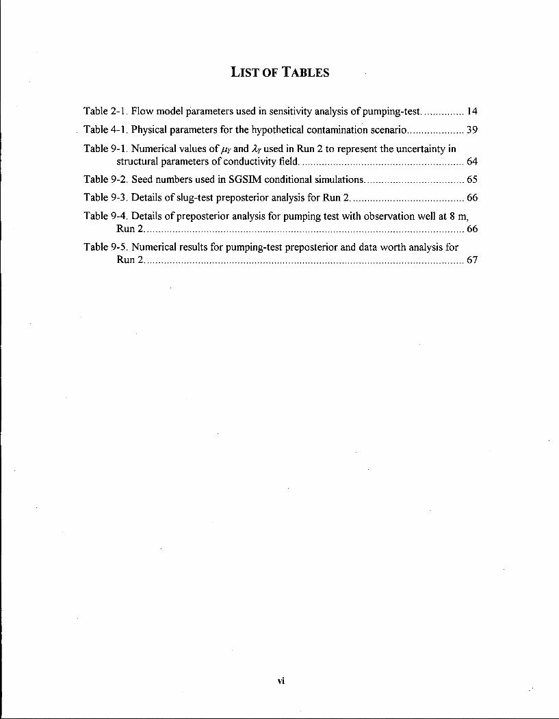
Table 2-1. Flow model parameters used in sensitivity analysis of pumping-test 14

Table 4-1. Physical parameters for the hypothetical contamination scenario 39

Table 9-1. Numerical values of and Xy used in Run 2 to represent the uncertainty in

structural parameters of conductivity field 64

Table 9-2. Seed numbers used in SGSIM conditional simulations 65

Table 9-3. Details of slug-test preposterior analysis for Run 2 66 Table 9-4. Details of preposterior analysis for pumping test with observation well at 8 m,

Run 2 66

Table 9-5. Numerical results for pumping-test preposterior and data worth analysis for Run 2 67

vi

L I S T O F F I G U R E S

Figure 1-1. Relative support volume of pumping test (A) and slug test (B). The dark shade indicates zones of strong influence, and light shade zones of weak influence 2

Figure 2-1. Setup of the numerical flow model used for estimation of pumping-test averaging volume. The pumping well is located in the center of a confined aquifer represented by square, 89x89 numerical grid with no-flow boundaries on all four sides. The sensitivity coefficients are calculated within 30x30 window centered around the pumping well 15

Figure 2-2. Maps of logarithm of sensitivity coefficients Ur calculated at dimensionless time t 0.35 (a), 0.70 (b), and 1.40 (c), for the "observation" well 12 gridblocks away from the pumping well 17

Figure 2-3. Hydraulic conductivity fields used for the calculations of the sensitivity coefficients Ur*. The white cross denotes the pumping well, and white dots show the location of the observation wells 19

Figure 2-4. Maps of logarithm of sensitivity coefficients Ur for homogeneous transmissivity field (a, b, c), and "organized" transmissivity field (d, e, f). Dimensionless pumping-test duration t = 1.40 20

Figure 2-5. Maps of logarithm of sensitivity coefficients Ur for heterogeneous transmissivity fields with exponential correlation structure, correlation length of 20 gridblocks, and o2 of 0.15 (a, b, c) and 0.75 (d, e, f). Dimensionless pumping-test duration t = 1.40 21

Figure 2-6. Idealized zonation of the pumping test averaging volume 22

Figure 3-1. Generic aquifer contamination problem 28

Figure 3-2. Flow chart for estimating data worth of slug test and pumping test 30

Figure 3-3. Decision tree used in prior (A) and preposterior (B) analysis 34

Figure 4-1. Maps of Y point variances and corresponding travel time histograms for the generic contamination scenario 42

Figure 4-2. Data worth of slug test and pumping test. Run 2 is a base simulation with stochastic parameters described in the text. Run 1 and Run 3 have mean of correlation length set to L/2 and L/8 respectively. Run 4 and Run 5 have variance set to 0.75 and 1.25, respectively 43

Figure 4-3. Preposterior section of the decision tree for two slug tests. 46

Figure 4-4. Data worth of one slug test, two slug tests, and pumping tests with the

observation well at the distance of 4, 6, and 8 m from the pumping well 47

Figure 7-1. Five blocks of the finite difference grid 58 Figure 8-1. Plot of the objective function F in T and S space 63

vn

A C K N O W L E D G M E N T S

I would like to express my gratitude to my supervisor Roger Beckie. Thanks to him my first brush with

advanced hydrogeology took place when I was still an undergrad, while taking his graduate course,.

Roger, through his guidance and encouragement, helped me to survive several long hours at the keyboard.

He always had time to answer my questions despite my bad habit of popping by his office without any

warning.

I am also glad that I had the opportunity to study under Leslie Smith. Leslie is, in my and several other

hydro-people opinion, the best instructor that we have ever had. His clear and insightful lectures

illustrated with several case studies helped me grasp even the most difficult concepts of groundwater flow

and transport. Additionally, I want to thank Alan Sinclair for introducing me to the field of mining

geostatistics, Greg Dipple for his comments and suggestion, and my office-mate Ned Clayton for his

discussions of data worth applications.

Finally I thank my wife Anna, who had to deal with me, the perpetual student, for long four years. I also

thank my parents, who gave me an example to follow through their academic achievements.

viii

1

1. Introduction Hydraulic conductivity can be measured in the lab or field using permeameter tests, piezocone tests, slug

tests and pumping tests. Unfortunately, the hydraulic conductivities measured by these different tests are

not directly comparable because they characterize the subsurface at different scales. It is important to

consider the scale of a measurement when evaluating its usefulness. From a practical point of view, one

would like to determine which measurement provides the information that is most useful and cost-

effective for the problem at hand. The objective of this thesis is to determine the worth of hydraulic

conductivity data measured at different scales from the perspective of a decision maker faced with a

practical problem.

A typical contamination problem is used to provide the context in which to evaluate the worth of hydraulic

conductivity data. Hydraulic conductivity is perhaps the most important parameter controlling

contaminant migration in groundwater (Harvey and Gorelick, 1995; Kupfersberger and Bloschl, 1995;

James and Gorelick, 1994). Regrettably, in most practical problems the hydraulic conductivity field is not

well characterized. Consequently, groundwater contamination problems are difficult to manage. From a

decision maker's perspective, the uncertainty in hydraulic conductivity translates into a risk that the

selected management alternatives will not be the most cost-effective.

Decision makers can reduce their risk of not choosing the most cost-effective alternatives if they first

collect additional data from the site before making their management decisions. I thus calculate the worth

of hydraulic conductivity data measured on different scales by comparing the reduction in the risk of

choosing the wrong alternative with the cost of collecting additional data.

The following investigation is restricted to the comparative worth of hydraulic conductivity measured by a

slug test and by a pumping test. These are perhaps the two most widely used field-based hydraulic

conductivity measurements.

The scale, or support volume, of a measurement is that volume of porous media which the measured value

characterizes. The support volumes can be illustrated by plots which show how the porous media at each

2

point around the sampling location influences the measured value. These influence plots can be

interpreted as spatial filters which show how a smaller-scale parameter is averaged to yield a larger-scale

parameter (Desbarats 1994; Beckie and Wang 1994). The support volume of the slug test has been

extensively studied (Wang, 1995; Beckie and Wang, 1994; Guyonnet et al., 1993), however the support

volume of a pumping test in a radially non-symmetric media is not well know. Consequently, in Section

2.4.3,1 conduct an in depth investigation of the averaging properties of pumping test.

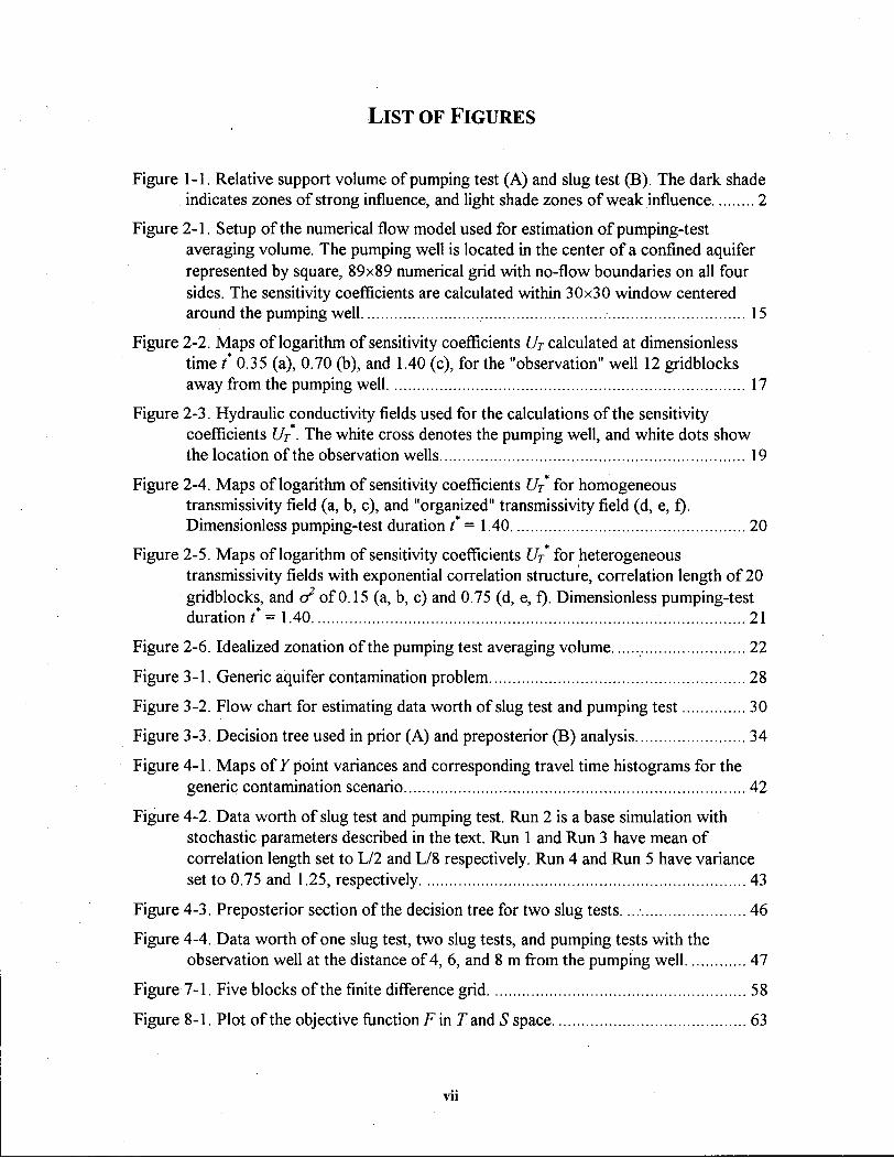
Figure 1-1 shows influence plots for hydraulic conductivity measured with a pumping test and a slug test

in a 2-d homogeneous confined aquifer. The darker areas indicate those zones of the aquifer that most

strongly influence the measured value. A slug test is a relatively small-scale measurement, which

characterizes a cylindrical volume of between 5 and 20 well radii around the piezometer. In contrast, the

support volume of a pumping test is much larger, on the order of the distance between the pumping well

and the observation piezometer.

observation well

pumping well

A. Pumping test B. Slug test

Figure 1-1. Relative support volume of pumping test (A) and slug test (B). The dark shade indicates zones of strong influence, and light shade zones of weak influence.

The notion that the smaller-scale slug test may have less value than a pumping test is reflected in the

sentiment of Osborn (1993) who states that "slug tests are much too heavily relied upon in site

characterization and contamination studies". If a site is heterogeneous, then a single, small-scale

measurement may not be representative of the overall site conditions. A measurement with a larger

3

support volume may, in contrast, better characterize the overall site conditions which control solute

migration. Recent field work suggests that small-scale slug tests generally provide estimates of hydraulic

conductivity that are lower than estimates from larger-scale pumping tests (Rovey and Cherkauer, 1995).

The use of smaller-scale conductivities could lead to erroneous travel time predictions. On the other hand,

the advantage of the slug test is that it is much less expensive than a pumping test. Pumping tests require

the installation of a pumping well, considerably longer monitoring than a slug test, and the potential need

to capture and treat contaminated well effluent. A suite of well-placed slug tests could, potentially, more

accurately resolve low and high permeability zones that are not resolved by a larger-scale measurement.

Chapter 2 presents an overview of common testing and data analysis techniques applicable to slug and

pumping test. A discussion of existing estimates of averaging volumes follows. The section ends with the

in depth investigation of a pumping test support volume using sensitivity analysis. Chapter 3 provides an

overview of the methodology developed to compare the data worth of slug and pumping tests. Here I

introduce the decision analysis framework, generic contamination scenario, and four step methodology

used in this thesis. The results of several numerical experiments are presented in Chapter 4. Finally in

Chapter 5 I summarize the major results and conclusions.

4

2. Averaging volumes of slug tests and pumping tests

2.1 Introduction

Before embarking on the data worth analysis, we need to investigate the averaging process inherent in

both slug and pumping tests, and its ramifications on the estimated hydraulic conductivities (K). A good

understanding of the slug/pumping test support or averaging volume is vital before application of any

geostatistical or updating method.

The averaging process is directly related to the scale over which a given measurement technique

integrates the hydraulic conductivity field. Rovey and Cherkauer (1995) investigated the hydraulic

conductivities estimated by slug tests, pumping tests, and those inverted from regional modeling studies.

They concluded that the magnitude of K increases with the scale of the measurement, and that this

relationship is similar to the scaling effect for dispersivity (Gelhar et al., 1992).

As noted by Beckie (1996) hydraulic conductivity can not be measured directly but must be inverted from

head observations using a measurement model. Therefore K estimates are dependent on the selected

measurement model, including its governing equation, boundary conditions, and domain size, and the

instrument used for hydraulic head observations.

Section 2.2 presents the three methods used to evaluate scale or the averaging volume of slug and

pumping test. Next, in Section 2.3 I discuss the field techniques and common measurement models

applicable to slug tests, and present the existing estimates of the slug test averaging volume. A summary

of pumping-test field techniques, popular measurement models, and existing estimates of the averaging

volume follows in Section 2.4. This section ends with a presentation of the numerical evaluation of

pumping test averaging volumes conducted as part of this thesis.

5

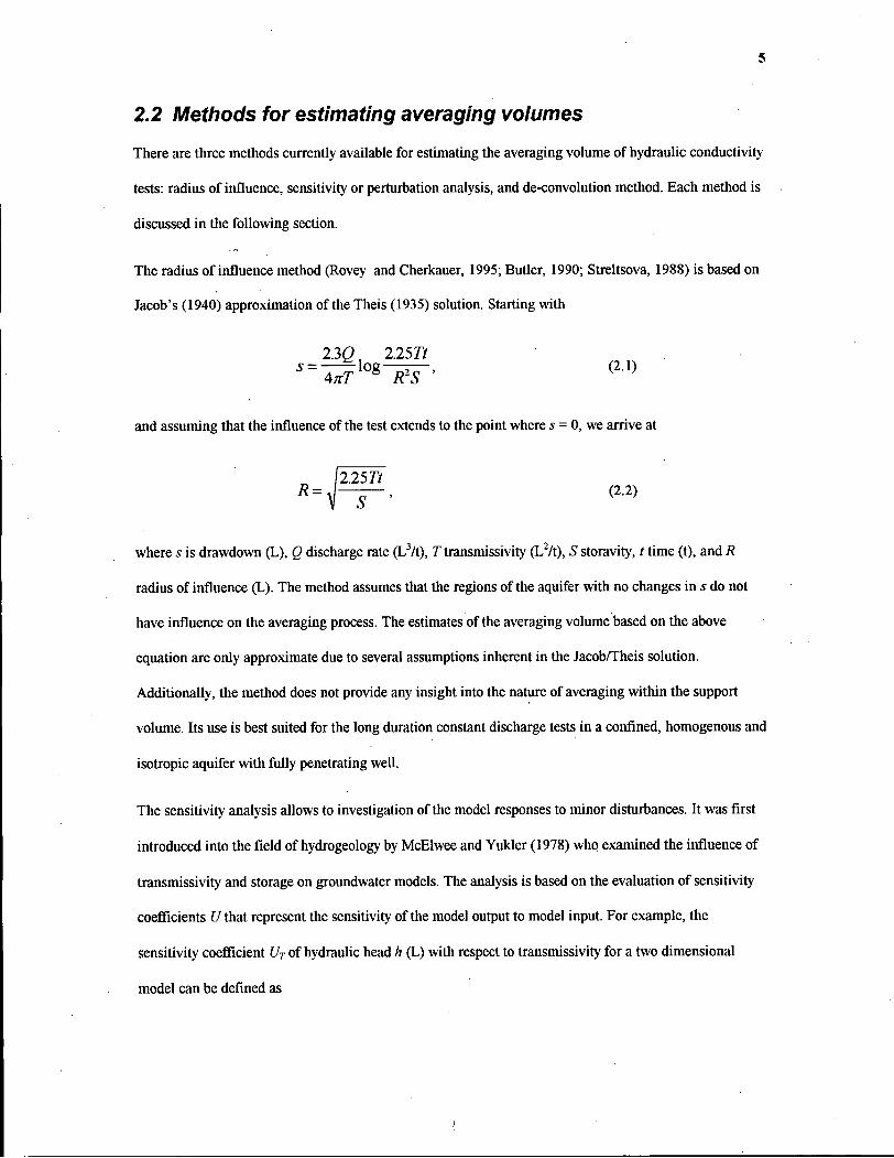
2.2 Methods for estimating averaging volumes

There are three methods currently available for estimating the averaging volume of hydraulic conductivity

tests: radius of influence, sensitivity or perturbation analysis, and de-convolution method. Each method is

discussed in the following section.

The radius of influence method (Rovey and Cherkauer, 1995; Butler, 1990; Streltsova, 1988) is based on

Jacob's (1940) approximation of the Theis (1935) solution. Starting with

23g 2.257/ ~4*T 8 R2S '

and assuming that the influence of the test extends to the point where s = 0, we arrive at

2.257/ R=y—=-, (2.2)

where s is drawdown (L), Q discharge rate (L3/f), T transmissivity (L2/t), S storavity, t time (t), and R

radius of influence (L). The method assumes that the regions of the aquifer with no changes in s do not

have influence on the averaging process. The estimates of the averaging volume based on the above

equation are only approximate due to several assumptions inherent in the Jacob/Theis solution.

Additionally, the method does not provide any insight into the nature of averaging within the support

volume. Its use is best suited for the long duration constant discharge tests in a confined, homogenous and

isotropic aquifer with fully penetrating well.

The sensitivity analysis allows to investigation of the model responses to minor disturbances. It was first

introduced into the field of hydrogeology by McElwee and Yukler (1978) who examined the influence of

transmissivity and storage on groundwater models. The analysis is based on the evaluation of sensitivity

coefficients U that represent the sensitivity of the model output to model input. For example, the

sensitivity coefficient UT of hydraulic head h (L) with respect to transmissivity for a two dimensional

model can be defined as

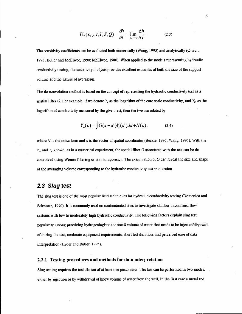
6

(2.3)

The sensitivity coefficients can be evaluated both numerically (Wang, 1995) and analytically (Oliver,

1993; Butler and McEhvee, 1990; McElwee, 1980). When applied to the models representing hydraulic

conductivity testing, the sensitivity analysis provides excellent estimates of both the size of the support

volume and the nature of averaging.

The de-convolution method is based on the concept of representing the hydraulic conductivity test as a

spatial filter G. For example, if we denote Yc as the logarithm of the core scale conductivity, and Ym as the

logarithm of conductivity measured by the given test, then die two are related by

where N is the noise term and x is the vector of spatial coordinates (Beckie, 1996; Wang, 1995). With the

Ym and Yc known, as in a numerical experiment, the spatial filter G associated with the test can be de­

convolved using Wiener filtering or similar approach. The examination of G can reveal the size and shape

of the averaging volume corresponding to the hydraulic conductivity test in question.

The slug test is one of the most popular field techniques for hydraulic conductivity testing (Domenico and

Schwartz, 1990). It is commonly used on contaminated sites to investigate shallow unconfined flow

systems with low to moderately high hydraulic conductivity. The following factors explain slug test

popularity among practicing hydrogeologists: the small volume of water that needs to be injected/disposed

of during the test, moderate equipment requirements, short test duration, and perceived ease of data

interpretation (Hyder and Butler, 1995).

2.3.1 Testing procedures and methods for data interpretation

Slug testing requires the installation of at least one piezometer. The test can be performed in two modes,

either by injection or by withdrawal of know volume of water from the well. In the first case a metal rod

(2.4)

2.3 Slug test

7

("slug") of known length and the diameter slightly smaller then the diameter of the piezometer is dropped

rapidly into the well. In the second case a bailer is submerged slowly in the well and then quickly lifted

from the piezometer. Sometimes the withdrawal test is termed "bail" test (CCME, 1994). Regardless of

the procedure, data collection involves measurements of hydraulic head versus time starting from the time

of injection/withdrawal. The measurements are taken either with an electric tape or with a pressure

transducer installed at the bottom of the well. The use of a pressure transducer is especially important in

highly conductive media, when the slug dissipation time is short.

Several methods are available for slug test data interpretation. Below, I briefly discuss the three most

popular techniques, namely Hvorslev (1951), Bouwer and Rice (1976), and Cooper et al. (1967). The

procedure developed by Hvorslev (1951) is among the most widely used (Domenico and Schwartz, 1990).

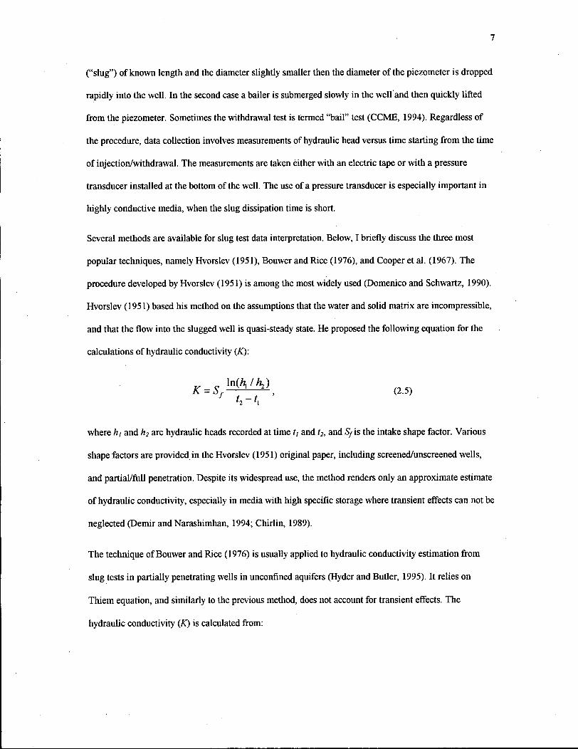
Hvorslev (1951) based his method on the assumptions that the water and solid matrix are incompressible,

and that the flow into the slugged well is quasi-steady state. He proposed the following equation for the

calculations of hydraulic conductivity (AT):

K = Sf ) \ , , (2.5)

where ht and h2 are hydraulic heads recorded at time tt and t2, and S/ is the intake shape factor. Various

shape factors are provided in the Hvorslev (1951) original paper, including screened/unscreened wells,

and partial/full penetration. Despite its widespread use, the method renders only an approximate estimate

of hydraulic conductivity, especially in media with high specific storage where transient effects can not be

neglected (Demir and Narashimhan, 1994; Chirlin, 1989).

The technique of Bouwer and Rice (1976) is usually applied to hydraulic conductivity estimation from

slug tests in partially penetrating wells in unconfmed aquifers (Hyder and Butler, 1995). It relies on

Thiem equation, and similarly to the previous method, does not account for transient effects. The

hydraulic conductivity (K) is calculated from:

8

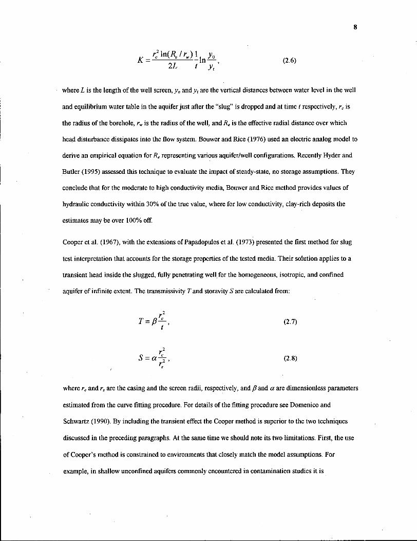
K = rc

2\n(Re/rw)\i y0

— — — - n — , 2L t

(2.6)

where L is the length of the well screen, ya and v, are the vertical distances between water level in the well

and equilibrium water table in the aquifer just after the "slug" is dropped and at time t respectively, rc is

the radius of the borehole, rw is the radius of the well, and Re is the effective radial distance over which

head disturbance dissipates into the flow system. Bouwer and Rice (1976) used an electric analog model to

derive an empirical equation for Re representing various aquifer/well configurations. Recently Hyder and

Butler (1995) assessed this technique to evaluate the impact of steady-state, no storage assumptions. They

conclude that for the moderate to high conductivity media, Bouwer and Rice method provides values of

hydraulic conductivity within 30% of the true value, where for low conductivity, clay-rich deposits the

estimates may be over 100% off.

Cooper et al. (1967), with the extensions of Papadopulos et al. (1973) presented the first method for slug

test interpretation that accounts for the storage properties of the tested media. Their solution applies to a

transient head inside the slugged, fully penetrating well for the homogeneous, isotropic, and confined

aquifer of infinite extent. The transmissivity T and storavity S are calculated from:

where rc and rs are the casing and the screen radii, respectively, and p and a are dimensionless parameters

estimated from the curve fitting procedure. For details of the fitting procedure see Domenico and

Schwartz (1990). By including the transient effect the Cooper method is superior to the two techniques

discussed in the preceding paragraphs. At the same time we should note its two limitations. First, the use

of Cooper's method is constrained to environments that closely match the model assumptions. For

example, in shallow unconfined aquifers commonly encountered in contamination studies it is

T (2.7)

S (2.8).

9

inapplicable. Secondly, the estimates of storavity obtained via Cooper method are not very reliable.

McElwee et al. (1995a, 1995b) used sensitivity analysis to show that the technique is much less sensitive

to S then to T. They stress that careful test design, including volume of water used and proper temporal

data collection, together with the application of the observation wells might improve the storavity

estimates.

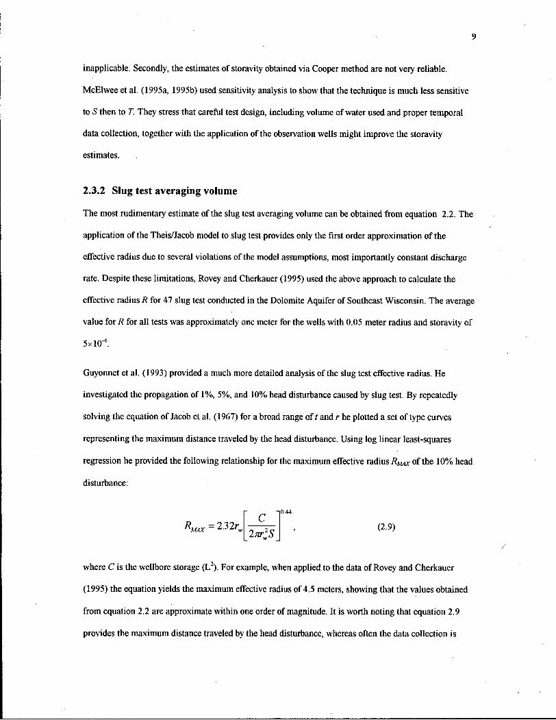
2.3.2 Slug test averaging volume

The most rudimentary estimate of the slug test averaging volume can be obtained from equation 2.2. The

application of the Theis/Jacob model to slug test provides only the first order approximation of the

effective radius due to several violations of the model assumptions, most importantly constant discharge

rate. Despite these limitations, Rovey and Cherkauer (1995) used the above approach to calculate the

effective radius R for 47 slug test conducted in the Dolomite Aquifer of Southeast Wisconsin. The average

value for R for all tests was approximately one meter for the wells with 0.05 meter radius and storavity of

5xl0-4.

Guyonnet et al. (1993) provided a much more detailed analysis of the slug test effective radius. He

investigated the propagation of 1%, 5%, and 10% head disturbance caused by slug test. By repeatedly

solving the equation of Jacob et al. (1967) for a broad range of t and r he plotted a set of type curves

representing the maximum distance traveled by the head disturbance. Using log linear least-squares

regression he provided the following relationship for the maximum effective radius RMAX of the 10% head

disturbance:

RM4X = 2.32rH

c n 0 4 4

2nrtS (2.9)

where C is the wellbore storage (L2). For example, when applied to the data of Rovey and Cherkauer

(1995) the equation yields the maximum effective radius of 4.5 meters, showing that the values obtained

from equation 2.2 are approximate within one order of magnitude. It is worth noting that equation 2.9

provides the maximum distance traveled by the head disturbance, whereas often the data collection is

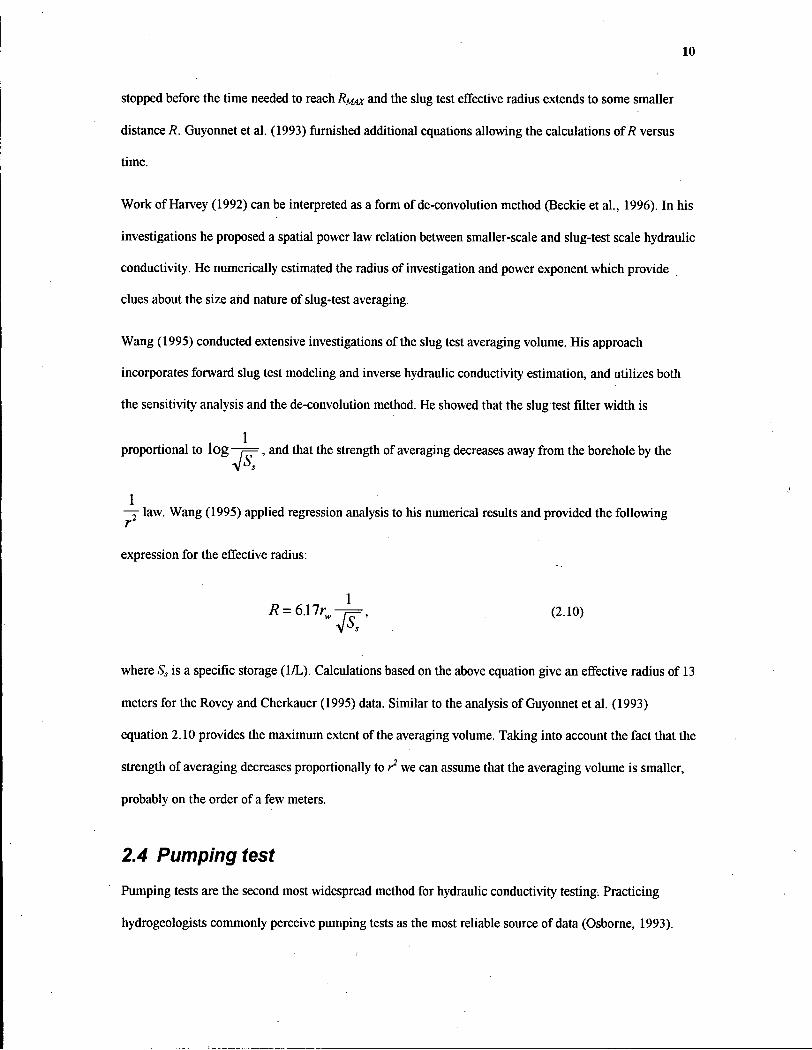
10

stopped before the time needed to reach R/MX and the slug test effective radius extends to some smaller

distance R. Guyonnet et al. (1993) furnished additional equations allowing the calculations of R versus

time.

Work of Harvey (1992) can be interpreted as a form of de-convolution method (Beckie et al., 1996). In his

investigations he proposed a spatial power law relation between smaller-scale and slug-test scale hydraulic

conductivity. He numerically estimated the radius of investigation and power exponent which provide

clues about the size and nature of slug-test averaging.

Wang (1995) conducted extensive investigations of the slug test averaging volume. His approach

incorporates forward slug test modeling and inverse hydraulic conductivity estimation, and utilizes both

the sensitivity analysis and the de-convolution method. He showed that the slug test filter width is

proportional to log ^ , and that the strength of averaging decreases away from the borehole by the

— law. Wang (1995) applied regression analysis to his numerical results and provided the following

expression for the effective radius:

where Ss is a specific storage (1/L). Calculations based on the above equation give an effective radius of 13

meters for the Rovey and Cherkauer (1995) data. Similar to the analysis of Guyonnet et al. (1993)

equation 2.10 provides the maximum extent of the averaging volume. Taking into account the fact that the

strength of averaging decreases proportionally to r2 we can assume that the averaging volume is smaller,

probably on the order of a few meters.

1

R = 6\lr 1

(2.10)

2.4 Pumping test

Pumping tests are the second most widespread method for hydraulic conductivity testing. Practicing

hydrogeologists commonly perceive pumping tests as the most reliable source of data (Osborne, 1993).

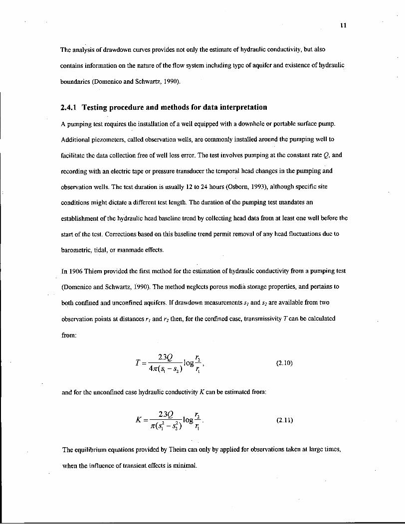
11

The analysis of drawdown curves provides not only the estimate of hydraulic conductivity, but also

contains information on the nature of the flow system including type of aquifer and existence of hydraulic

boundaries (Domenico and Schwartz, 1990).

2.4.1 Testing procedure and methods for data interpretation

A pumping test requires the installation of a well equipped with a downhole or portable surface pump.

Additional piezometers, called observation wells, are commonly installed around the pumping well to

facilitate the data collection free of well loss error. The test involves pumping at the constant rate Q, and

recording with an electric tape or pressure transducer the temporal head changes in the pumping and

observation wells. The test duration is usually 12 to 24 hours (Osborn, 1993), although specific site

conditions might dictate a different test length. The duration of the pumping test mandates an

establishment of the hydraulic head baseline trend by collecting head data from at least one well before the

start of the test. Corrections based on this baseline trend permit removal of any head fluctuations due to

barometric, tidal, or manmade effects.

In 1906 Thiem provided the first method for the estimation of hydraulic conductivity from a pumping test

(Domenico and Schwartz, 1990). The method neglects porous media storage properties, and pertains to

both confined and unconfined aquifers. If drawdown measurements 5/ and s2 are available from two

observation points at distances r, and r2 then, for the confined case, transmissivity T can be calculated

from:

r = , J o g - , ( i . i o )

and for the unconfined case hydraulic conductivity K can be estimated from:

K= 2 % l o g - ^ . (2.11)

The equilibrium equations provided by Theim can only by applied for observations taken at large times,

when the influence of transient effects is minimal.

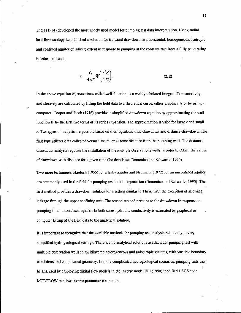
12

Theis (1934) developed the most widely used model for pumping test data interpretation. Using radial

heat flow analogy he published a solution for transient drawdown in a horizontal, homogeneous, isotropic

and confined aquifer of infinite extent in response to pumping at the constant rate from a fully penetrating

infinitesimal well:

s = -Q-W\ ' r S

TF. • ( 2 1 2 ) ATtJ

In the above equation W, sometimes called well function, is a widely tabulated integral. Transmissivity

and storavity are calculated by fitting the field data to a theoretical curve, either graphically or by using a

computer. Cooper and Jacob (1946) provided a simplified drawdown equation by approximating the well

function W by the first two terms of its series expansion. The approximation is valid for large t and small

r. Two types of analysis are possible based on their equation, time-drawdown and distance-drawdown. The

first type utilizes data collected versus time at, or at some distance from the pumping well. The distance-

drawdown analysis requires the installation of the multiple observations wells in order to obtain the values

of drawdown with distance for a given time (for details see Domenico and Schwartz, 1990).

Two more techniques, Hantush (1955) for a leaky aquifer and Neumann (1972) for an unconfined aquifer,

are commonly used in the field for pumping test data interpretation (Domenico and Schwartz, 1990). The

first method provides a drawdown solution for a setting similar to Theis, with the exception of allowing

leakage through the upper confining unit. The second method pertains to the drawdown in response to

pumping in an unconfined aquifer. In both cases hydraulic conductivity is estimated by graphical or

computer fitting of the field data to the analytical solution.

It is important to recognize that the available methods for pumping test analysis relate only to very

simplified hydrogeological settings. There are no analytical solutions available for pumping test with

multiple observation wells in multilayered heterogeneous and anisotropic systems, with variable boundary

conditions and complicated geometry. In more complicated hydrogeological scenarios, pumping tests can

be analyzed by employing digital flow models in the inverse mode. Hill (1990) modified USGS code

MODFLOW to allow inverse parameter estimation.

13

2.4.2 Existing estimates of pumping test averaging volume

Whereas the slug test involves observations of head dissipation over a short time period that depends on

the properties of tested aquifer, the pumping test requires pumping at a constant discharge rate for longer

periods. Therefore, unlike the slug-test averaging volume, the area of the pumping-test averaging volume

and the radius of influence depends on the test duration (Desbarats, 1992). The maximum extent of the

cone of depression at any given time can be approximated from equation 2.1. This approach was used by

Rovey and Cherkauer (1995) for their approximation of pumping-test scale.

Various researchers investigated the averaging inherent in a pumping test. Butler (1988) and Butler and

McElwee (1990) used sensitivity analysis combined with analytical solutions for a well embedded in a disc

of different transmissivity from the transmissivity of the surrounding area. Butler (1991a) provided a

semi-analytical solution for drawdown in a system with a linear strip of different transmissivity. Although

insightful, the above work suffers from the assumptions of radial symmetry and simple geometry, and does

not treat the relation between smaller scale (eg. slug-test scale) and pumping-test scale conductivity

directly. Butler (1991b) used a stochastic analysis of transmissivities estimated from pumping tests, but he

did not consider the averaging volume explicitly.

Desbarats (1992) examined the relation between the smaller-scale transmissivities and block-scale

transmissivity inverted with a single well pumping test. He expressed the pumping-test scale measurement

as the power weighted average of the smaller-scale quantities, and empirically estimated the weighting

exponent. His approach is somewhat limited due to the steady-state assumption employed in the analysis.

Beckie at al. (1996) pointed out that Desbarats' (1992) analysis can be interpreted as the de-convolution

method.

Oliver (1990) used a sensitivity analysis to determine the weighting function which represents the

relationship between single well pumping-test estimated transmissivity and smaller scale aquifer

transmissivities. He found that the averaging area and the radius of investigation increased with test

duration. Oliver extended his work in his 1993 paper, where, using the sensitivity approach he derived the

Frechet derivatives for the effect of two-dimensional variations in transmissivity on drawdown at the

14

observation well. His work showed that the effect of radially non-symmetric heterogeneities on drawdown

for the case of a pumping test with an observation well is much more complex then predicted by Butler

(1988).

In the next section I present numerical estimates of pumping test averaging volume using the sensitivity

analysis. The results are an extension of the work conducted by Oliver (1993).

2.4.3 Pumping test volume via sensitivity analysis

The main goal of the work presented in this section is to provide insight into the averaging process

inherent in the pumping test by extending the results of Oliver (1993). In his work he examined the

influence of small non-homogeneities on pumping-test induced drawdown at the observation well, but he

did not account for the measurement model nor did he consider heterogeneous AT fields. To fully

understand pumping-test averaging one has to include one of the measurement models, like Theis (1935)

or Cooper and Jacob (1942), and investigate the spatial relation between the small scale hydraulic

conductivity and pumping-test averaged hydraulic conductivity inverted with the measurement model

(Beckie, 1996). It is also important to consider the impact of heterogeneous AT fields, both spatially

correlated and "organized", on the shape and structure of the averaging volume.

The following analysis utilized a two dimensional transient finite difference flow simulator for a confined

aquifer (see Appendix I). All simulations were conducted on the 89x89 square grid with the pumping well

located in the center of the model, and no flow boundaries on all four sides (Figure 2-1). The duration of

the pumping was short enough to guarantee a negligible influence of the boundaries on drawdown. The

model parameters are summarized in Table 2-1.

Transmissivity T (m'Vs) 1.6x10"2

Storavity S 1.0x10"2

Pumping rate Q (mJ/s) 0.16 Test duration (hr) 21.78

Numerical gridblock x and y size (m) 25

Table 2-1. Flow model parameters used in sensitivity analysis of pumping-test.

15

Window used for sensitivity calculations —\

\

• ®

30 gridblocks

Rnnnriarips nf • " ^ ^ the flow model

89 gridblocks

• - pumping well ® - observation well

Figure 2-1. Setup of the numerical flow model used for estimation of pumping-test averaging volume. The pumping well is located in the center of a confined aquifer represented by square, 89x89 numerical grid with no-flow boundaries on all four sides. The sensitivity coefficients are calculated within 30x30 window centered around the pumping well.

First I verify the sensitivity analysis used in this thesis against the results of Oliver (1993). The sensitivity

coefficients of hydraulic head with respect to changes in transmissivity, as defined in equation 2.3, are

calculated in the 30x30 window centered around the pumping and "observation" wells (see Figure 2-1)

using the following procedure:

1. run the transient flow simulator with the non-perturbed transmissivity field, record base head

h'base at the "observation well" at each time step /,

2. go to gridblock ij and perturb the transmissivity Ty by a small value AT,

16

3. run the transient flow simulator with the well pumping at the rate Q, record head h'y at the

"observation" well at each time step t,

4. restore the value of transmissivity at gridblock ij,

5. repeat steps 2 to 4 for all gridblocks within the 30x30 window.

The sensitivity coefficients are calculated as:

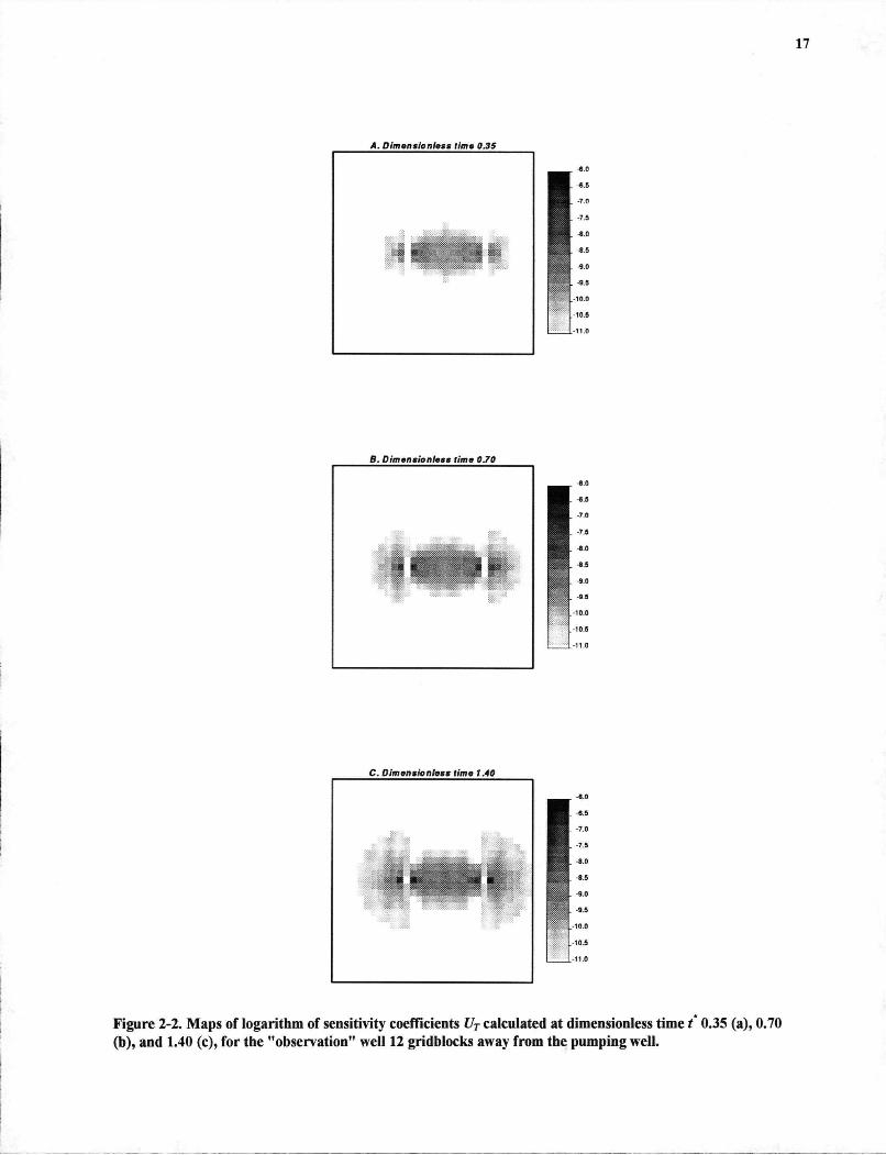
for each time step t and gridblock ij. The maps of sensitivity coefficients calculated for time steps 13 (r =

0.35), 15 (r* = 0.70), and 17 (r* = 1.40), for observation well 12 gridblocks away from the pumping well

are presented in Figure 2-2. t* denotes dimensionless time

f=-%. (2.14,

These results are in a full agreement with the ones presented by Oliver (1993, Figure lb).

However useful, the analysis of pumping-test volume based on the sensitivity coefficients defined in

equation 2.3 and calculated above does not account for the measurement model associated with the

analysis of pumping-test data. To include the measurement model in the analysis one has to examine the

spatial distribution of the sensitivity coefficients UT' of pumping-test averaged transmissivity I9*"' with

respect to smaller scale transmissivity T, defined as follows

U*(x,y\T,S,Q) = ^—=Y\m——. (2.15)

Beckie et al. (in press, 1996) demonstrated that the sensitivity coefficients UT* are directly related to the

measurement filter function G (equation 2.4).

17

A. Dimensionless time 0.35

-6.0

B. Dimensionless time 0.70

Figure 2-2. Maps of logarithm of sensitivity coefficients UT calculated at dimensionless time t 0.35 (a), 0.70 (b), and 1.40 (c), for the "observation" well 12 gridblocks away from the pumping well.

18

Numerically, the computations are similar to those outlined above in steps 1 to 5, with the addition of the

automatic curve fitting of the numerical time-drawdown curve to the measurement model time-drawdown

curve. Here I use Theis (1934) measurement model as the one that closely matches the experimental setup.

The details of automatic inversion of the pumping-test drawdown data using downhill simplex algorithm

(Press et al., 1989) are provided in Appendix II. The sensitivity coefficients UT" are calculated as:

rpptest rpptest

r T * base ii

U«= AT • < 2 1 6 )

where T*J£' is the transmissivity inverted from drawdown in the non-perturbed transmissivity field, and

TjJtest is the transmissivity inverted from drawdown computed for the field perturbed at gridblock ij.

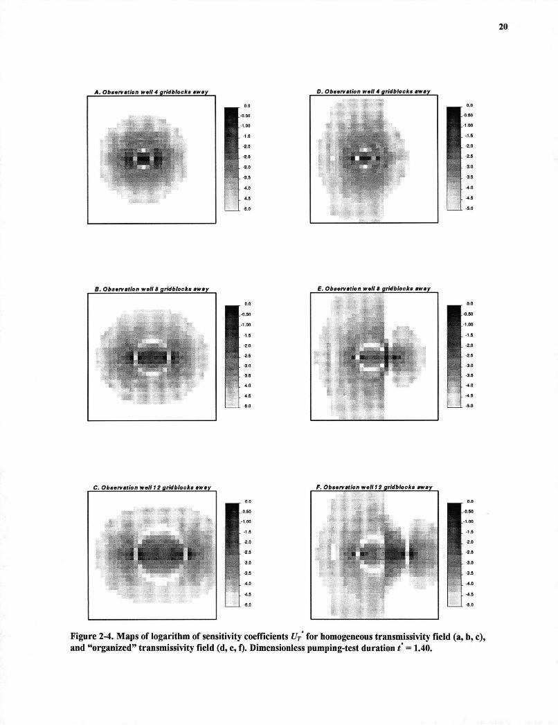
Sensitivity coefficients defined in equation 2.15 are calculated for several cases. In case one I plot the log

sensitivity coefficients for a homogeneous transmissivity field with the "observation" wells 4, 8, and 12

gridblocks away from the pumping well (Figure 2-4 a, b, c). Next I consider an "organized" transmissivity

field (Figure 2-3 a). Sensitivity coefficient maps (Figure 2-4 d, e, f) are calculated for a linear strip 9

gridblocks in width centered on the pumping wells, and embedded in the lower transmissivity matrix.

Finally I examine two heterogeneous transmissivity fields with exponential correlation structure,

correlation length A = 20 gridblocks, and a2 equal to 0.15 (Figure 2-3 b) and a2 = 0.75 respectively. Maps

of log sensitivity coefficients UT* for both transmissivity fields are shown in Figure 2-5.

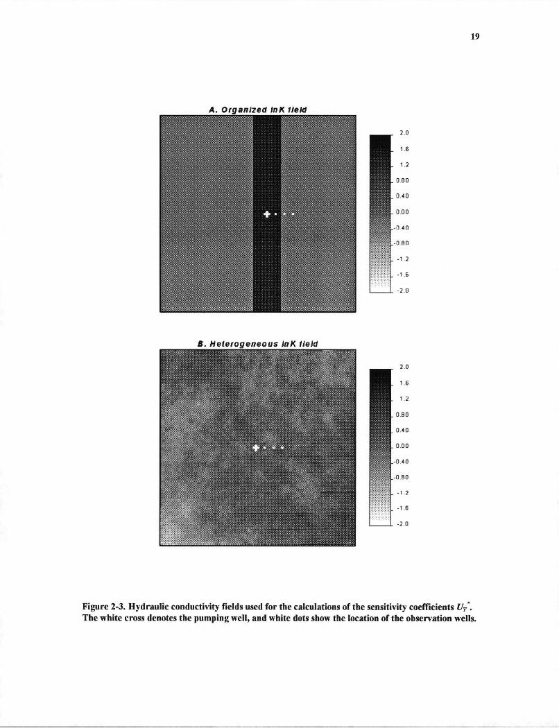
Figure 2-3. Hydraulic conductivity fields used for the calculations of the sensitivity coefficients Ur". The white cross denotes the pumping well, and white dots show the location of the observation wells.

A. Observation well 4 gridblock* mwty D. ObMerwlion wall 4 gridblocks twmy

Figure 2-4. Maps of logarithm of sensitivity coefficients UT' for homogeneous transmissivity field (a, b, and "organized" transmissivity field (d, e, f). Dimensionless pumping-test duration t = 1.40.

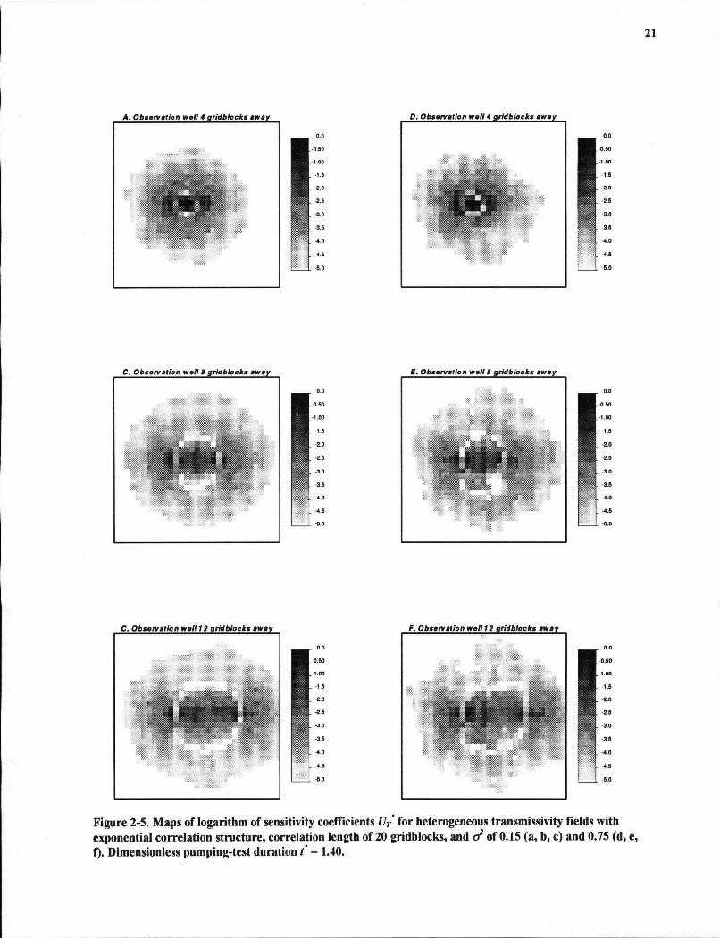
Figure 2-5. Maps of logarithm of sensitivity coefficients UT' for heterogeneous transmissivity fields with exponential correlation structure, correlation length of 20 gridblocks, and a2 of 0.15 (a, b, c) and 0.75 (d, e, f). Dimensionless pumping-test duration t = 1.40.

22

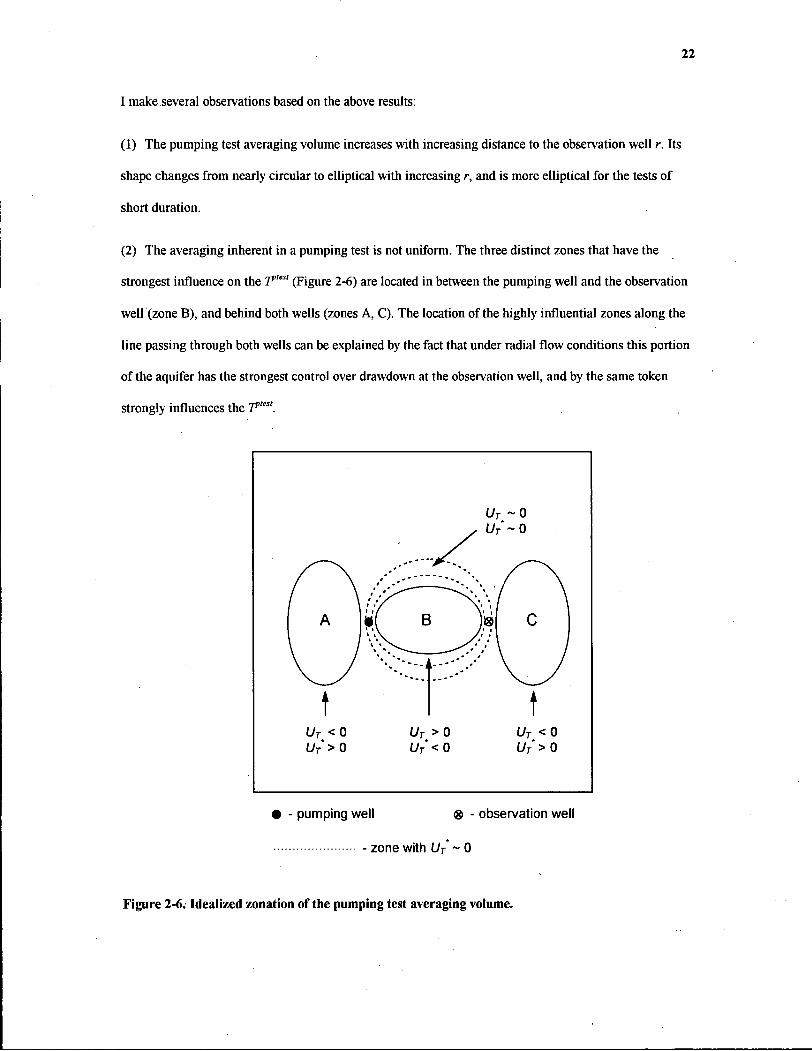
I make several observations based on the above results:

(1) The pumping test averaging volume increases with increasing distance to the observation well r. Its

shape changes from nearly circular to elliptical with increasing r, and is more elliptical for the tests of

short duration.

(2) The averaging inherent in a pumping test is not uniform. The three distinct zones that have the

strongest influence on the V"est (Figure 2-6) are located in between the pumping well and the observation

well (zone B), and behind both wells (zones A, C). The location of the highly influential zones along the

line passing through both wells can be explained by the fact that under radial flow conditions this portion

of the aquifer has the strongest control over drawdown at the observation well, and by the same token

strongly influences the 7**"*.

UT ~0 UT~0

UT < 0 UT> 0

UT > 0 UT'< 0

UT < 0 UT'> 0

• - pumping well ® - observation well

- zone with UT ~ 0

Figure 2-6. Idealized zonation of the pumping test averaging volume.

(3) Different zones around the pumping well and the "observation" well have different influence on Tpt"t.

The influence zonation is constant for both homogeneous and heterogeneous transmissivity fields

considered here.

• In zone A (Figure 2-6) UT has a negative sign showing that a small zone of higher T behind

the pumping well will result in higher head at the "observation" well. This can be explained

by the fact that in the section of the aquifer with lower, non-perturbed transmissivity the

gradient must increase in order to maintain a constant radial flux into the well. The change

in gradient has an immediate impact on the Tpte". The UT' is positive showing that the

existence of the zone of higher T behind the pumping well translates into smaller value of

transmissivity inverted from the smaller but steeper (in time) drawdown from the

"observation" well.

• In zone B (Figure 2-6) UT is positive and UT' negative. Higher conductivity zone in-between

the pumping and the "observation" wells results in weaker gradient around the "observation"

well, larger head drops, and in turn larger value of V"est after the inversion of time-

drawdown data.

• In zone C (Figure 2-6), behind the "observation" well, UT is negative and Uj positive.

Although the result is similar as for zone A, the physical explanation is slightly different.

Groundwater encounters a smaller resistance to flow in a zone of higher T behind the

"observation" well, and that causes a smaller gradient around the zone with perturbed T.

However, downgradient from the non-uniformity there is an increase in gradient to conserve

mass in the non-perturbed transmissivity field. This corresponds to smaller hydraulic head

drops at the "observation" well, and in turn is manifested in lower estimates of Tpte".

• Sections of the aquifer at the border of zone B, marked with hatched lines on Figure 2-6,

have no impact on transmissivity estimated from pumping-test despite their proximity to the

pumping and "observation" wells. Heterogeneity in these zones will not influence 7*""'.

24

(4) The averaging volume of the pumping test increases with the test duration as predicted by all

discussed methods. However, contrary to the results of Butler (1988), even at large times V"est depends on

the zone in-between the pumping and "observation" wells.

(5) For heterogeneous transmissivity fields, the shape of the pumping-test averaging volume disintegrates

(Figure 2-4 d, e, f, and Figure 2-5). This suggests that for heterogeneous aquifers it may be impossible to

define one unique averaging volume. The above observation has implications for the methods used to

incorporate pumping-test conductivity information, which I discuss in Section 3.4.3. However, some

characteristic features, like high sensitivity along the line joining the two wells and ABC zonation, are

still distinguishable even for the case with heterogeneity strength cr7 = 0.75.

The above analysis suffers from several simplifying assumptions, including two dimensional flow,

idealized confined aquifer, single observation well, and exclusive use of Theis measurement model for

drawdown inversion. Especially, in the case of non fully penetrating wells and/or unconfined aquifer with

strong vertical flow, the averaging volume might have much more complicated three-dimensional

structure. The structure would be further distorted in the case of simultaneous inversion of data from

multiple "observation" wells. However, despite the limitations, the above analysis is unique in its kind by

providing the first insight into the pumping test averaging for the non-radially symmetric case and a

single "observation" well.

2.5 Conclusion

The slug test is a small scale, inexpensive field technique used for hydraulic conductivity testing. The

averaging volume is circular with the effective radius proportional to the borehole radius and inversely

proportional to the Ss'°5.

Pumping-test estimated hydraulic conductivity is a larger scale, more costly measurement. The size of

averaging volume is proportional to the duration of the test and the distance between the pumping and

"observations" wells. The shape of the averaging volume changes from circular to elliptical with the

increasing distance between the "observation" and pumping well, and with decreasing test duration. The

25

zones that influence the transmissivity estimated from pumping tests are located behind the pumping and

"observation" wells, and in-between the boreholes.

In the next section I introduce the methodology that allows to compare the worth of hydraulic conductivity

measurements with respect to their scale.

26

3. Methodology for establishing data worth

3.1 Introduction

Having described the averaging properties of slug and pumping test I now develop a methodology that

allows to compare both tests. In Section 3.2 I provide a brief introduction to decision analysis that forms a

foundation of my analysis, and introduce the concept of data worth as applied to groundwater studies.

Section 3.3 contains a description of a generic contamination scenario that is used in slug and pumping

3.4. Here I discuss the uncertainty model of hydraulic conductivity, the "exhaustive" updating method,

and prior and preposterior analysis.

I take a decision maker's perspective and thus use decision analysis (Benjamin and Cornell, 1970) to

evaluate the relative worth of slug-test and pumping-test hydraulic conductivity data. Decision analysis

views an engineering problem as a sequence of decisions between alternatives with the objective of

maximizing the decision maker's expected utility. This utility is typically measured in monetary units. The

objective is formalized in an objective function

where O is the decision maker's utility, and B, C and R are the total benefit, cost, and probabilistic cost or

risk, associated with the chosen decision alternatives. The risk term reflects that an alternative may not

achieve the engineering goal and hence be classified as a failure. Risk is quantified here as

test data worth evaluation. The details of four step methodology employed in this thesis follow in Section

3.2 Decision analysis

® = B-C-R, (3.1)

(3.2)

where P/is the probability of failure and C/is the cost of failure.

27

In practice, one evaluates the expected value of the objective function, E(<t>) for every decision alternative,

where E is the expectation operator taken over every possible state of nature. One then selects the

alternative with the highest expected <S>:

Freeze and coworkers developed a decision analysis framework for groundwater problems (Freeze et al,

1990, 1992; Massmann et al, 1991; Sperling et al, 1992; James and Freeze 1993). In many groundwater

contamination problems, the benefits B are zero. The costs are those associated with the selected

remediation or preventative actions such as pumping wells or cut-off walls. A typical failure occurs when

a contaminant reaches a compliance boundary or exceeds a threshold concentration. When a failure

occurs, the responsible party will often be fined by the regulator and will be required to pay for remedial

measures.

Intuitively, one can better select the lowest-cost management alternative if more information about the

uncertain hydrogeological system is available. Therefore, data only have worth if they aid in the selection

of the proper course of action among alternatives (Freeze et al, 1992; James and Freeze, 1993; James and

Gorelick, 1994).

A data-worth calculation is performed before any data is collected. In the so-called prior analysis, one first

determines the alternative with the highest expected O given the current information. Next, in the

preposterior analysis, one hypothetically collects data and determines the highest expected <£> with sample

information. The worth of data is defined as the difference between the objective function calculated in the

preposterior and prior analysis. Data have worth if <5 after the hypothetical data collection is greater than

O before data collection.

The work in this thesis is most closely related to James and Gorelick (1994), who present a methodology

to determine the optimal number and location of water-quality samples from a polluted aquifer. In

contrast, I focus on hydraulic conductivity and the issue of the scale at which it is measured. I compare the

worth of hydraulic conductivity measured by a slug-test and pumping-test at a fixed sampling location.

28

3.3 Generic contamination scenario

I use the following hypothetical scenario to introduce my methodology. Although it is simplified, it

contains many elements of a typical field problem. The proposed methodology can be easily extended to

accommodate more complicated hydrogeological environments.

Consider a fully confined aquifer with flow essentially in two dimensions (Figure 3-1). There is negligible

vertical flow because of the aquifer's large aerial extent compared to its thickness. The horizontal flow is

in the southern direction. There is no flow across E and W boundaries. Advection is the dominant

transport mechanism with negligible influence of hydrodynamic dispersion and diffusion.

groundwater flow direction

I I I I C site of potential contamination }

• K ? ?

X K ? ?

• K ? ?

• K ? ?

compliance boundary

• existing piezometer

X location of proposed test

Figure 3-1. Generic aquifer contamination problem.

29

There is a potential for aquifer contamination across the whole northern boundary due to upstream

activities by the potential responsible party. Accordingly, the regulator has designated the southern

boundary of the property to be a compliance surface. If contamination is detected at the compliance

surface in a time less than a critical travel time tcrit, then the responsible party will be fined and forced to

remediate.

The potential responsible party faces a decision between two possible alternatives: action and no action.

The action option is costly but is here for simplicity assumed to reduce the chance of non-compliance to

zero. Action alternatives with uncertain outcomes can also be accommodated by the methodology. On the

other hand, if the hydraulic conductivity is sufficiently high, the no action alternative could lead to a fast

travel time and thus trigger the even more costiy fines and remedial measures.

I assume that slug-test data from three fully-penetrating piezometers are already available. Three

observation wells are typically installed in the initial stages of a site investigation to determine head

gradients. Together with the information on local geology, the wells provide for the current estimate of the

hydraulic conductivity field and the travel time. Taking another measurement of hydraulic conductivity

could reduce the potential responsible party's risk of selecting the wrong alternative.

3.4 Four step methodology

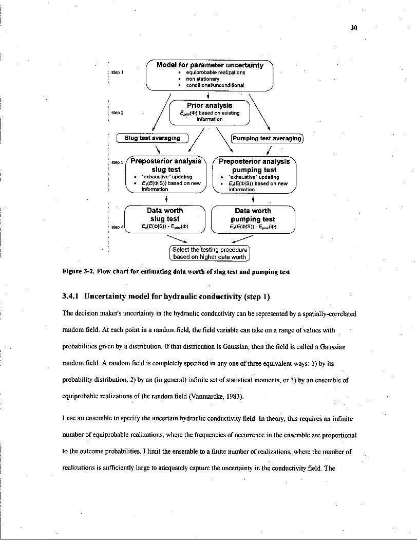
In Figure 3-21 summarize the four-step methodology used to determine the worth of an additional

hydraulic conductivity measurement. In step one I construct an uncertainty model for the hydraulic

conductivity field. The uncertainty model is then used in step two to carry out a prior analysis. Here I use

decision analysis to select the most economical alternative based on the current knowledge of the

hydraulic conductivity field. Next, in step three, I carry out a preposterior analysis for both a slug and

pumping test. Preposterior analysis allows us to evaluate the impact of sample information on the

management decision before the tests are actually performed. The analysis utilizes the concept of

exhaustive updating and accounts for the scales at which hydraulic conductivity is measured. Finally,

based on prior and preposterior analysis, I obtain a worth of sample and the more cost-effective sampling

method is selected. The following sections provide details on each step of our methodology.

30

step 1 Model for parameter uncertainty

• equiprobable realizations • non stationary • conditional/unconditional

-

step 2 Prior analysis

EpnA®) based on existing information

( Slug test averaging )

\ ^ step 3 ^Preposterior analysis'

slug test • "exhaustive" updating • £,(E(0|S)) based on new

information . | Data worth slug test

s t e p 4 l E,(E(<I>|S)) - Epl)0r(O)

(Pumping test averaging)

, Preposterior analysis

pumping test • "exhaustive" updating • £,(E(<D|S)) based on new

information

I . Data worth

pumping test E,(E(<D|S)) - Ep^O)

Select the testing procedure I based on higher data worth

Figure 3-2. Flow chart for estimating data worth of slug test and pumping test

3.4.1 Uncertainty model for hydraulic conductivity (step 1)

The decision maker's uncertainty in the hydraulic conductivity can be represented by a spatially-correlated

random field. At each point in a random field, the field variable can take on a range of values with

probabilities given by a distribution. If that distribution is Gaussian, then the field is called a Gaussian

random field. A random field is completely specified in any one of three equivalent ways: 1) by its

probability distribution, 2) by an (in general) infinite set of statistical moments, or 3) by an ensemble of

equiprobable realizations of the random field (Vanmarcke, 1983).

I use an ensemble to specify the uncertain hydraulic conductivity field. In theory, this requires an infinite

number of equiprobable realizations, where the frequencies of occurrence in the ensemble are proportional

to the outcome probabilities. I limit the ensemble to a finite number of realizations, where the number of

realizations is sufficiently large to adequately capture the uncertainty in the conductivity field. The

31

appropriate number of realizations is estimated by examining the rate at which ensemble-based statistics

change as the number of realizations increases.

Below I describe how I construct the ensemble of realizations that represent the uncertain hydraulic

conductivity field. In keeping with hydrogeological practice and experience, I cast the problem in terms of

7= In AT, the logarithm of hydraulic conductivity (Freeze, 1975).

First, on the basis of an exploratory data analysis I propose a model for the spatial structure of the

conductivity field. These models are called variograms in the geostatistics literature and covariances in

linear estimation theory (Kitanidis and Vomvoris, 1983). Usually there is insufficient data to warrant

more than a simple model of spatial structure. In the example to follow below, I assume that field data

support the use of an exponential model of spatial correlation.

Next, I use the data to identify the parameters for the model of spatial structure. The most common

parameters that appear in the models of spatial structure are the mean /ur, the variance ay2, and Ay, the

correlation length. In the absence of prior information, the maximum likelihood method initially proposed

by Kitanidis and Vomvoris (1983) can be used to estimate the structural parameters. Kitanidis and

coworkers show that this approach is not affected by the biases which plague many parameter

identification procedures (Kitanidis and Vomvoris 1983; Hoeksema and Kitanidis 1984; Kitanidis and

Lane 1985).

With limited field data, the structural parameters are difficult to estimate and thus uncertain. Kitanidis

and Lane (1985) show that the correlation length can be particularly difficult to estimate when the

separation distance between data points is small compared to the correlation length of the log-conductivity

field. Russo and Jury (1987) obtain similar results. On the other hand, if the data points are spaced at the

distances greater than the correlation length the estimates of the spatial statistics are marred by aliasing

errors (Beckie, 1996). I thus estimate the mean and variance of the spatial-structure parameters jjy and Ar,

and assume that they have a Gaussian distribution. I can thereby account for the uncertain structural

parameters when I generate realizations for the ensemble.

32

Lastly, I generate conditional realizations for the ensemble according to the spatial structure given by the

structural model (e.g. variogram). To account for the uncertain parameters of the structural model, several

sets of realizations are simulated, each set with different structural parameters. The number of fields

within a set is selected to correspond to the probability of occurrence of the structural parameters as given

by the Gaussian distribution identified in the previous step. In this way, the ensemble itself accounts for

uncertainty in the structural parameters. This contrasts an approach where one accounts for uncertainty in

the parameters using a Bayesian distribution (Kitanidis 1986; Rubin and Dagan 1992).

I use algorithms published by Deutsch and Journel (1992) to generate realizations conditioned on the

measurement data. In this work, the hydraulic conductivity realizations are conditioned on log-

conductivity measurements only.

3.4.2 Prior analysis (step 2)

Before proceeding with the prior analysis, I must define all possible outcomes of the objective function <J>.

In the scenario which I present above, the objective function $ can take on three values after the

management decision has been made. If the no action alternative (A„a) is selected and a failure does not

occur, then <t>(Ana) will have a high value as a consequence of not spending on preventive action.

However, if no action is selected and the contaminant reaches the compliance surface before tcrit, then

large fines and cleanup costs will reduce <f>(A„a) to a low value. If the action alternative is selected (A a) the

objective function will take on an intermediate value ®(Aa) reflecting the cost of preventative action such

as a cutoff wall, grout curtain, or pump and treat system. If, in contrast to our example, the outcome of the

action alternative is uncertain then an additional risk term would further lower the value of ®(Aa).

The decision is made using the expected value of the objective function based upon existing information.

In the prior analysis of this example, the value of the objective function is uncertain for the no action

alternative ®(A„a) only, because the success or failure of this alternative is uncertain. Our methodology

closely follows that of Benjamin and Cornell (1972) and James (1992). The prior analysis is represented

33

in the upper section of the decision tree (Figure 3-3). I refer the reader to Benjamin and Cornell (1972) for

a detailed explanation of decision trees.

The two branches emerging from the decision node (the black square) of prior analysis decision tree in

Figure 4 represent the two alternatives available to the responsible party. The upper, action alternative

branch, labeled^,,, ends with the single value of the objective function ®(Aa), since the value of the

objective function is assumed to be known with certainty if this alternative is selected. The lower branch

of the prior analysis corresponds to the no action alternative (A„a). It ends with the chance node (black

circle) that reflects our uncertainty in the state of nature, namely the true travel time. The dotted lines

emerging from the chance node denote the multiple realizations of the log-conductivity field and

corresponding possible travel times.

To evaluate the expected value of the objective function for the no action alternative (A na) we must

calculate the travel time in each log-conductivity realization and determine if it is less than the critical

travel time tcrU. To do this, I first compute the total discharge Q through the realization using a 2-d steady-

state flow simulator. Next, I calculate the travel time as:

/ = nLA I Q, (3.3)

where n is porosity, L is distance between the source and the compliance surface, and .4 is the cross-

sectional area of the aquifer. Alternatively, the travel time can be calculated by utilizing an advection-

dispersion transport simulator. I assign the <&{Ana) value to each field based on the tcrit failure criterion.

The expected value of the objective function for the no action alternative, Em($>(Ana)), can thus be

calculated, where m indicates expectation taken over all log-conductivity realizations.

34

Figure 3-3. Decision tree used in prior (A) and preposterior (B) analysis.

The prior analysis ends by comparing the objective function assigned to the decision branches^ andAna.

I select the decision alternative that maximizes economic benefits of the responsible party and set the

corresponding objective function to Eprior(<!>). The decision is thus made in the light of all existing

information about the hydraulic conductivity.

Before we proceed to step three of our methodology I have to introduce the concept of exhaustive updating

which I use in the preposterior analysis. The exhaustive updating allows us to condition the log-hydraulic

conductivity fields on measurements with different support.

35

3.4.3 Exhaustive updating

I use an exhaustive updating approach to condition my ensemble of hydraulic conductivity fields on the

measurement data. The method is conceptually identical to the method used by James and Gorelick

(1994). I condition the ensemble by culling out those realizations that do not match the measurement data

to a specified tolerance. For example, when a slug-test measured conductivity of Kstug is measured at a

point x, then I exhaustively search through all members of the ensemble and remove those realizations for

which the hydraulic conductivity at point x is outside the range of K„iug - 6K< K(x) < Kslug + 5K, where

SK is the tolerance. The tolerance allows us to account for both the finite precision at which the hydraulic

conductivity is stored in the computer and for measurement errors. Conditioning on pumping-test

measurements is somewhat more involved.

To condition on a pumping-test measurement, I first numerically simulate a pumping-test in each

realization of the ensemble, and invert the resulting drawdown-time curve using a standard confined

aquifer Theis solution. The inversion is performed using downhill simplex method described by Press et

al. (1989). For details see Appendix II. I then cull out all realizations for which the numerically-

determined hydraulic conductivity does not match the measured conductivity within a specified tolerance.

The exhaustive, ensemble-based updating differs from approaches which rely upon a mean and variogram

or covariance function characterization of the ensemble (e.g. Delhomme 1979; Hachich and Vanmarcke

1983; Kitanidis and Vomvoris 1983; Dagan 1985; Kitanidis 1986; Graham and McLaughlin 1989;

Harvey and Gorelick 1995). Often the mean and covariance of the unconditioned ensemble can be

represented by simple functions. However, because the means and covariances of the updated ensemble

are non-stationary, they are more difficult to represent. As noted by Harvey and Gorelick (1995), a field

discretized into nb=nxxny gridblocks requires covariance matrices of size nbxnb. For example, a lOOx 100

gridblock field requires a 10000 x 10000 covariance matrix. Exhaustive updating does not use covariances,

and thus avoids this difficulty.

Another advantage of the exhaustive updating is its capability to fully incorporate all complexities of the

pumping-test averaging. The covariance or conditional simulation based methods provide only

36

approximate conditioning on the pumping-test measurement because they utilize an idealized

representation of the pumping-test averaging. This approach was used by Deutsch and Journel (1994) who

represented pumping-test measurements as the spatial power average in their simulated annealing

algorithm. However, as I show in Section 2.4.3, the shape and structure of the pumping-test averaging

volume strongly depends on the spatial distribution of the hydraulic conductivity, and will vary for Y

realizations generated with the same structural parameters. The exhaustive updating method, via forward

pumping-test simulations, has the capability to account for pumping test averaging unique to each

realization in the ensemble.

Both exhaustive updating and variogram and covariance-based updating approaches can be extended to

accommodate measurements, such as head or concentration, that are functionally related to the hydraulic

conductivity field. For example, to condition on head measurements, the head field would be numerically

simulated in each log-conductivity field realization, and then compared to the measured head. Those log-

conductivity field realizations for which the head fields did not match within a tolerance would be culled

out of the ensemble.

To update with measurements that are functionally related to the hydraulic conductivity field using

variogram and covariance-based methods requires that the covariogram or covariance between the

hydraulic conductivity field and measurement be known. Often these correlations are calculated using

linearizations of the governing flow and transport equations that are accurate to a low order in the

variance of the log-hydraulic conductivity (Kitanidis and Vomvoris 1983; Dagari 1985; Graham and

McLaughlin 1989). This linearization step has the potential to introduce errors that do not appear in the

exhaustive updating procedure.

Perhaps the greatest disadvantage of exhaustive updating is the need to generate large numbers of

realizations to produce stable statistics. The generation of log-conductivity realizations and simulation of

pumping tests in turn requires significant computational time. In a sense, there is a trade-off between the

computer-memory-intensive covariance matrix approaches and the cpu-intensive exhaustive methods.

Like any Monte-Carlo method, exhaustive updating is ideally suited for parallel processing.

37

3.4.4 Preposterior analysis (step 3)

The preposterior analysis allows us to evaluate the economic benefits of sampling before the data are

actually collected. I perform a preposterior analysis for both a slug and pumping test. The analysis is

virtually the same for both tests except for the conditioning step explained above. The procedure is

represented graphically in the lower part of the decision tree in Figure 3-3.

The essential idea of the preposterior analysis is to first calculate the expected value of the objective

function given that a sample outcome S has been observed, and then to average the objective function over

all possible sample outcomes. As assumed in the prior analysis, the objective function is known with

certainty if the action alternative is selected, and the expected value of no action alternative can be

calculated by averaging over all possible realizations of the log-conductivity field.

In contrast to the prior analysis, the expected value of the objective function for the no action alternative is

now calculated with the ensemble conditioned on the observed data. This is illustrated in the decision tree

of Figure 4. The n possible sample outcomes are indicated with the branches labeled S, to S„ which

originate from a chance node. Each of these branches ends with a decision node representing the action or

no action alternative.

For each sample outcome S, to S„, we must calculate the expected value of the objective function for the

no action alternative. For example, this expectation is indicated at the decision node connected to branch

S1; in Figure 3-3. Note however that at this decision point the ensemble is conditioned on the outcome S1;,

such that only those m' fields consistent with the observed Si remain in the ensemble. Thus we calculate

the expected value of the objective function Em{<b(A„a\Si)) using the m' realizations, where \S] indicates

conditioning on sample outcome Sj. As in the prior analysis, we select that alternative that maximizes the

economic benefits given a sample outcome 5 ;:

(3.4)

This value is assigned to the decision node ending the branch Si.

38

The above procedure is repeated n times for each possible sample outcome. In some cases, hydraulic

conductivity testing will increase the chance of failure and the action alternative will be selected. In

others, the risk will decrease and the no action options will be chosen. Overall, each of the E(<t>\Sj)

assigned to the decision nodes will reflect how the responsible party would act if the sample outcome were

known.

The preposterior analysis ends by incorporating the uncertainty in the possible sample outcome S. The

expected expected value of the objective function is calculated as:

Es(E(^\S)) = fJP(Si)E(0\Si), (3.5) 1=1

where P(Sj) is probability of collecting a sample with the outcome 5„ and subscript S indicates expectation

taken over all possible sample outcomes. I perform the above calculation for the slug test and pumping

test. Consequently, both the slug test and pumping test are assigned a value ES(E(<&\ S)).

3.4.5 Data worth (step 4)

In the final step of my methodology, I calculate the data worth of a pumping test and slug test performed

at the predefined location. The data worth represents the economic gain due to prospective sampling. It is

calculated as:

Worth = Es(EmS))-Eprior<<S>). (3.6)

If the worth of data is negative, then the data should not be collected. If the worth is positive, then the data

with the highest worth minus the cost of sampling should be collected.

In the following Chapter I present a numerical example. It demonstrates the application of my

methodology to the generic scenario introduced above.

39

4. Worth of slug test and pumping test

4.1 Introduction

In this chapter I apply the four step methodology developed in Chapter 2 to a generic contamination

scenario. The main goal of the analysis is to quantify the impact of the averaging process on the worth of

the hydraulic conductivity measurements. In Section 4.2 I evaluate the data worth of a single slug test

compared with a single pumping test. Section 4.3 contains the comparison of two slug test measurements

with one pumping test. A discussion of model limitations and assumptions follows in Section 4.4. Finally,

in Section 4.5 I present the conclusions emerging from the numerical experiments.

4.2 Data worth of a single slug test versus a single pumping test

I assume the following physical parameters (Table 4-1) for the hypothetical contamination scenario

introduced on Figure 2-1.

Aquifer thickness (m) 10 hydraulic conductivity - piezol (m/s) 1.4x10"5

aquifer length/width L (m) 130 hydraulic conductivity - piezo2 (m/s) 9.6 x10'6

porosity n 0.35 hydraulic conductivity - piezo3 (m/s) 2.1x10-B

storage coefficient S 1x10-3 gradient i 3.9 x10"3

Table 4-1. Physical parameters for the hypothetical contamination scenario.

A uniform 65 x 65 block grid is superimposed on the site where the gridblock dimensions are set to

2mx2m. This gridblock size corresponds to the averaging volume of a slug test with the effective radius of

about lm, in agreement with the assumptions of Rovey and Cherkauer (1995) and numerical analysis of

Wang (1995) and Guyonnet et al. (1993). Therefore, the slug test scaling effects are implicit in my model,

whereas the pumping-test averaging will be considered explicitly. The duration of the proposed pumping

test is six hours with a pumping rate of 0.001 m3/s. Under these conditions, the influence of the

boundaries on the simulated cone of depression is negligible.

The structural parameters of the log-conductivity field are estimated from the existing slug-test data and

from local geology. The estimates of the parameters are: mean log-conductivity iuY= -9.62, the variance of

the log conductivity ay2= 1.00, and correlation length AY = Z-/4, where L is the field length on a side.

40

These parameters are only estimates and are uncertain. I assume that both the mean pY and the correlation

length AY have Gaussian distributions with coefficients of variation of 0.05 and 0.2 respectively. The large

coefficient of variation for Ay reflects the difficulty in estimating this parameter from field observations.

To simplify my presentation, I assume that the variance of the log-conductivity field ay2 is known with

certainty.

My ensemble consists of 500 realizations of the log-conductivity field. The spatial structure is modeled

with an exponential covariance function

C(x) = <j2r exp(-\x\/Xr), (4.1)

where x is the separation distance (Deutsch and Journel 1992). I generate the realizations using the

sequential Gaussian algorithm from Deutsch and Journel (1992). The ensemble consists of 25 sets of 20

realizations, where each set of realizations is generated with a different combination of the structural

parameters ur and Ay. All realizations are conditioned on the three existing slug-test measurements.

Each log-conductivity field serves as an input to the flow simulator. First I calculate a steady state flow

field under the constant head boundaries at S and N parts of the site. The resulting head distribution is

used to estimate the contaminant travel time, and serves as an input to the transient pumping-test

simulation. The transient simulation provides the time-drawdown curve for each of the hypothetical

observation wells. The curves are inverted using Theis (1934) solution. Then the numerical values for

travel time, conductivity at the test location (slug test conductivity), and pumping-test conductivities are

recorded, and the above steps are repeated for all fields constituting the ensemble.

After the decision is made, the objective function can take on one of three possible values. If the action

alternative (Aa) is selected, <$>(Aa) is known with certainty and is here set to $500,000. If the no action

alternative (A„a) is selected and a failure occurs, ®(Ana) is set to $-200,000. If no failure occurs Q>(A„a) is

set to $800,000. The selected values are similar to ones used by James (1992) and provide a good estimate

of O for an average contaminated site. However the sensitivity analysis shows that the relative data worth

of slug and pumping tests is independent of the assigned cost, therefore my calculations are valid for any

41

values of <£>. The critical time W is set to 4 years. I perform five simulation runs. Run 2 is a base-case

simulation with the structural parameters listed above. I investigate the role of correlation length on data

worth in runs 1 and 3, and the influence of the heterogeneity strength as measured by ay2 in runs 4 and 5.

In each run, I calculate the worth of pumping-test measurements taken at different scales. I can increase

the scale of the pumping test by moving the observation piezometer further from the pumping well.

4.2.1 The effect of "exhaustive" updating

Before presenting the results of data worth calculations I examine the effect of "exhaustive" updating on

the point variance of the log transmissivity ensemble. The point variances are calculated for each

gridblock ij as

o £ = - ,• (4.2)

" n

where

1 n

and n is the number of realizations. A map plot of cr/y provides an estimate of the spatial uncertainty in

the log transmissivity field and is directly related to the uncertainty in the contaminants travel time. In

Figure 4-11 present three maps of point variance calculated for set of realizations in Run 2 together with

histograms of log travel time. Map A represents prior uncertainty in the Y field, and maps B and C show

the uncertainty after updating on a single slug test and pumping test, respectively. The inspection of the

plots reveals that, although reducing the point variance to zero at the measurement location, a single slug

test provides a minor reduction in the Y uncertainty. The reduction of uncertainty increases with, like in

the case of pumping test, larger sampling volume. It is also worth noting that the pumping test does not

reduce the point variance to zero at the measurement location. In fact, in the model presented here, one

could consider pumping test as a "soft" measurement similar to geophysical data.

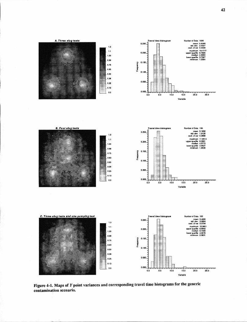
A. Three stug tests Travel time histogram Numberot Data 1500

B. Four slug tests Travel time histogram Number of Data 150

C. Three slug tests and one pumping test Travel time histogram Number o( Data 150

Figure 4-1. Maps of Y point variances and corresponding travel time histograms for the generic contamination scenario.

43

4.2.2 Numerical results

In Figure 4-2 I plot the worth of the slug-test measurement and pumping-test measurements taken with

piezometers located 4, 6, and 8 m from the pumping well. The detailed numerical results for run 2 are

summarized in Appendix III. The figures display the worth of cost-free measurements. In effect, I display

the dollar value of the information content of the measurement. The worth of a measurement.can be

determined by subtracting the cost of the measurement from the worth displayed in Figure 4-2.

$35 --$30 -I 1 1 1

Slug Pump Test Pump Test Pump Test Test OWat4m OWat6m OWat8m

$30 -I 1 1 ; 1 Slug ' Pump Test Pump Test Pump Test Test OW at 4m OW at 6 m OW at 8 m

Figure 4-2. Data worth of slug test and pumping test. Run 2 is a base simulation with stochastic parameters described in the text. Run 1 and Run 3 have mean of correlation length set to L /2 and L/8 respectively. Run 4 and Run 5 have variance set to 0.75 and 1.25, respectively.

I first make three observations based upon the results in Figure 4-2:

(1) For the scenario considered here, the dollar-value of information in pumping-test measurements is

greater than that of slug tests. The base-case results (run 2, Figure 4-2) indicate that the dollar value of the

44

information from a pumping test with an observation well 8 meters away is 54 % greater than the value of

information from a slug test. This confirms our intuition - the larger-scale pumping-test measurement

provides a better estimate of the hydraulic conductivity experienced by the plume and by the same token,

reduces the uncertainty in the travel time more strongly than slug tests. Thus a larger-scale measurement

improves the probability that the decision maker will select the most cost-effective alternative.

(2) The value of the information from a pumping test increases as the distance from the pumping well to

the observation well increases. For the base run 2, this value is $68,000, $74,000, and $79,000 for a

pumping test with the observation piezometer 4, 6, and 8 meters away from the pumping well respectively.

This result has practical implications. When a pumping test is selected as the preferred measurement

alternative, the observation well should be placed sufficiently far to achieve a large averaging volume.

(3) The worth of a pumping test is consistently higher than the worth of a slug test under all combinations

of structural parameters investigated here.

I expect the data worth to be affected by the spatial structure of the log-conductivity field. Dagan (1990)

demonstrates that when the plume is much smaller than the correlation length, the conductivity

measurements strongly influence predictions, whereas when the plume is large compared to the

correlation length of the field, the measurements have less influence on transport predictions. I thus expect

that fields with long correlation lengths relative to the plume width will yield measurements with greater

worth. For my problem, the plume width is implicitly assumed to be equal to the width of the area of

potential contamination. The results of runs 1, 2, and 3, displayed in top panel of Figure 4-2, show that as

the correlation length increases, the value of information in each measurement increases. The proportional

increase in value is approximately uniform for each measurement.

The effect of heterogeneity strength ay2 on the value of the information is less clear to me (Figure 5,

bottom panel). The strength of heterogeneity increases from a lowest value in run 4, oy2 = 0.75, to cry2 =

1.00 in run 2, and to ay2 = 1.25 in run 5. The results indicate that the value of information in the largest-

scale pumping test decreases as the strength of heterogeneity increases, whereas the value of information

in a slug test increases with increasing strength of heterogeneity. Perhaps the pumping test results may be

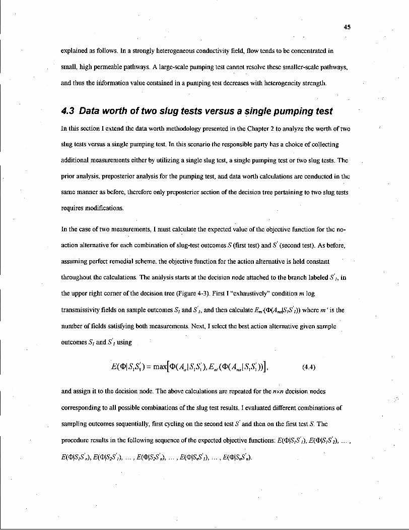
45

explained as follows. In a strongly heterogeneous conductivity field, flow tends to be concentrated in

small, high permeable pathways. A large-scale pumping test cannot resolve these smaller-scale pathways,

and thus the information value contained in a pumping test decreases with heterogeneity strength.

4.3 Data worth of two slug tests versus a single pumping test

In this section I extend the data worth methodology presented in the Chapter 2 to analyze the worth of two

slug tests versus a single pumping test. In this scenario the responsible party has a choice of collecting

additional measurements either by utilizing a single slug test, a single pumping test or two slug tests. The

prior analysis, preposterior analysis for the pumping test, and data worth calculations are conducted in the

same manner as before, therefore only preposterior section of the decision tree pertaining to two slug tests

requires modifications.

In the case of two measurements, I must calculate the expected value of the objective function for the no-

action alternative for each combination of slug-test outcomes S (first test) and S' (second test). As before,

assuming perfect remedial scheme, the objective function for the action alternative is held constant

throughout the calculations. The analysis starts at the decision node attached to the branch labeled S i, in

the upper right corner of the decision tree (Figure 4-3). First I "exhaustively" condition m log

transmissivity fields on sample outcomes St and S\, and then calculate Em{0(A„a\S,S;)) where m' is the

number of fields satisfying both measurements. Next, I select the best action alternative given sample

outcomes S; and S) using

£ ( W . " ) = ™i®(AJSXlEA®(AJSX))l (4.4)

and assign it to the decision node. The above calculations are repeated for the nxn decision nodes

corresponding to all possible combinations of the slug test results. I evaluated different combinations of

sampling outcomes sequentially, first cycling on the second test S' and then on the first test S. The

procedure results in the following sequence of the expected objective functions: E(<&\SiS',), E(d>\SiS'2), ...',

E(®\S,S'„), £(<W',), ... , E(®\S2S'„), EmS£'i), ... , £(<W'n).

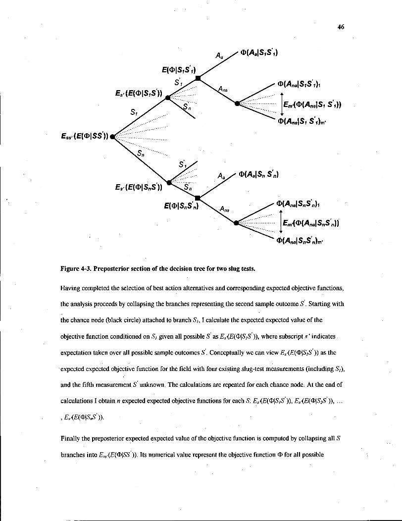
46

A / 0(A,|S,S t)

E(0|S,S f)

Si

£ S ( £ ( 0 | S , S ) )

s1

ESS-(£(<D|SS))

ES(£(<D|S„S))

E ( 0|S nS n)

Em(<D( na|S, S,))

0(A.a|S, S'i)m'

®(Ana\SnSnh

Em>mAna\S„S'n))

0(Ana\SnSn)m-

Figure 4-3. Preposterior section of the decision tree for two slug tests.

Having completed the selection of best action alternatives and corresponding expected objective functions,

the analysis proceeds by collapsing the branches representing the second sample outcome S. Starting with

the chance node (black circle) attached to branch Si, I calculate the expected expected value of the

objective function conditioned on 5; given all possible S' as ES(E(Q)\S,S )), where subscript s' indicates

expectation taken over all possible sample outcomes S'. Conceptually we can view Es{E(tyS]S )) as the

expected expected objective function for the field with four existing slug-test measurements (including Sj),

and the fifth measurement S unknown. The calculations are repeated for each chance node; At the end of

calculations I obtain n expected expected objective functions for each S: Es{E(<b\S,S )), ES{E(Q?\S2S )), ...

,Es{E(0\S^)).

Finally the preposterior expected expected value of the objective function is computed by collapsing all S

branches into Ea(E(®\SS )). Its numerical value represent the objective function O for all possible

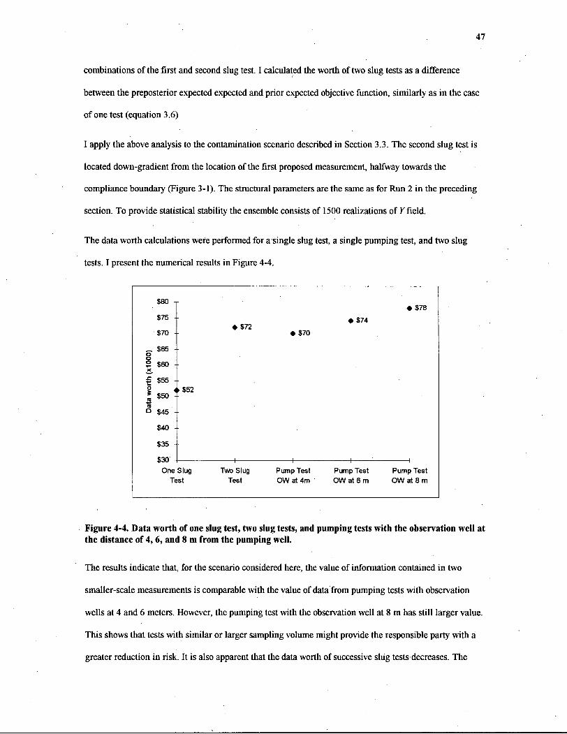
47

combinations of the first and second slug test. I calculated the worth of two slug tests as a difference

between the preposterior expected expected and prior expected objective function, similarly as in the case

of one test (equation 3.6)

I apply the above analysis to the contamination scenario described in Section 3.3. The second slug test is

located down-gradient from the location of the first proposed measurement, halfway towards the

compliance boundary (Figure 3-1). The structural parameters are the same as for Run 2 in the preceding

section. To provide statistical stability the ensemble consists of 1500 realizations of Y field.

The data worth calculations were performed for a single slug test, a single pumping test, and two slug

tests. I present the numerical results in Figure 4-4.

Figure 4-4. Data worth of one slug test, two slug tests, and pumping tests with the observation well at the distance of 4 ,6 , and 8 m from the pumping well.

The results indicate that, for the scenario considered here, the value of information contained in two

smaller-scale measurements is comparable with the value of data from pumping tests with observation

wells at 4 and 6 meters. However, the pumping test with the observation well at 8 m has still larger value.

This shows that tests with similar or larger sampling volume might provide the responsible party with a

greater reduction in risk. It is also apparent that the data worth of successive slug tests decreases. The

48

difference between the data worth of two and one slug test is $20,000, less than 50% of the value of single

measurement.

4.4 Model assumptions and limitations

The generic contamination scenario used in the preceding sections, although similar to a "real world" site,

is a simplified picture of reality. The limitations in the flow, transport, and decision analysis models are

discussed below.

I assume a 2D flow system of simple geometry with one geostatistical structure of the transmissivity field,

and fully penetrating wells: The impacts of unconfined conditions, vertical flow, leakage, partially

penetrating wells, and multilayer hydrostratigraphy are not considered here. However I believe that to

evaluate the data worth of a typical pumping test one has to work with the setup that closely matches the

assumptions of the most common pumping-test measurement model, namely Theis (1934) solution. More

involved problems, with for example "organized" transmissivity fields or variable geometry, would require

the evaluation of drawdown data based on hydrogeological experience and switching between different

measurement models. This type of analysis would be beyond the automatic curve matching employed in

my work.

The travel time calculations based on Darcy's Law utilize the most simple transport model available. By

assuming that the whole upstream boundary could be contaminated I treat the site as a single flow tube,

and calculate the average time needed for the contaminants front to reach the compliance surface.

Obviously I do not consider the effects of dispersion, diffusion, or retardation. However, all these

phenomena should have the same impact on travel time regardless of the measurement taken, and

therefore the use of the simplest transport model is justified.

A similar argument applies to the assumptions in the decision analysis model. Here I do not consider time

dependency of the objective function, greater number of remedial alternatives, or risk prone Aa. More

involved decision analysis model has equal impact on data worth of both slug and pumping tests, and does

49

not influence their relative worth. Additionally, by reducing the number of model parameters, the

simplifications allow to focus on the averaging issue.

The impact of location on test's data worth is not treated in my work directly. The computer intensive

nature of the "exhaustive" updating currently precludes this type of analysis. For example, to calculate a

map of pumping-test data worth one would have to repeat the data-worth analysis for each gridblock -

total of 65x65x500 transient flow simulations. However, without carrying out the numerical analysis, I

argue that the comparison of the data worth of the two tests is valid for the generic contamination scenario

used in this thesis. Because the plume width is equal to the site width and the aquifer has regular

geometry, there is no preferential location for the test. The worth of the measurement can only be reduced

by the interference with the preexisting slug tests, but maps of point variance plotted in Figure 4-1

indicate that the pre-selected testing location is siifficiently far removed from other piezometers. In fact,

one could probably move the testing location several gridblocks towards the existing piezometers without

any significant drop in data worth. This hypothesis is further supported by the additional calculations for

the second slug test (Section 4.3). I treated the second slug as the single measurement, and calculated its

data worth within $1,000 of that of the first measurement.

To apply my results in practice, one must account for the cost of the measurement. Consider the results

from run 2 displayed in Figure 4-2. If the cost of a slug test were less than the $50,000 value of the

information contained in the slug test, then it would be worthwhile to perform a slug test. Note however

that the assumed economic parameters have a strong influence on the data worth (James and Freeze

1993). Consequently, the worth of a slug test or pumping test depends upon the context in which it is

evaluated.

The data-worth methodology can be easily extended to account for more complex scenarios. Both flow and

travel time calculations could be performed using elaborate transient 3D flow and transport codes. The

decision analysis component of my method could be enhanced to incorporate time dependence of the

objective function, additional alternatives, and other sources of uncertainty. I could also utilize the method

of exhaustive updating to condition not only on hydraulic conductivity data, but also on hydraulic head

50

and concentration measurements from the existing and proposed wells. However, any increase in

complexity would require an increase in computational resources.

4.5 Conclusions

Data worth calculations indicate that, for the generic contamination scenario considered here, the value of

information contained in a single slug test is lower then in a single pumping test. Additionally, the

pumping test worth increases with the increasing distance between the observation and pumping wells.

The results are consistent under various combinations of the structural parameters controlling the

transmissivity field. This indicates that, by providing a greater reduction in the contaminant travel, time

uncertainty, the larger scale measurements have a greater impact on the decision making process.

The worth of information contained in two slug tests is comparable with the one provided by the pumping

test of moderate sampling volume. However, the larger-scale pumping tests proved to be more valuable.

Also, the worth of a slug test decreased as the number of measured locations increases. Therefore a longer-

duration pumping test with sufficiently far removed observation well may provide more information than

few slug tests.

Several simplifying assumption inherent in the generic contamination scenario do not invalidate the data

worth calculations. Most notably the numerical values of the objective function and the predefined

location of the tests have negligible impact on the relative worth of slug and pumping test. The results of

the analysis should be directly applicable to the sites with characteristics similar to ones considered here.

51

5. Summary and conclusion The objective of this thesis is to perform a data worth comparison of hydraulic conductivity measurements

taken at different scales. Here I compare the two most commonly used field techniques, slug tests and

pumping tests. The tests are compared in a typical contamination scenario using an empirical/numerical

approach.

The thesis contribution is threefold, comprising the investigation of the averaging properties of the

pumping test, the development of the data worth methodology applicable to measurements taken at

different scales, and application of the methodology to a generic contamination problem.

The averaging properties of pumping test are studied using sensitivity analysis. My results permit me to

make several observations. In a homogeneous aquifer the size of the pumping-test averaging volume

increases with the test duration and with distance r between the pumping and observation wells. Its shape

changes from circular to elliptical as r increases and pumping duration decreases. The averaging volume

exhibits a characteristic zonation, with zones of greatest influence on estimated conductivity located

behind the pumping and observation wells, and in-between the boreholes. With increasing heterogeneity,

the shape and structure of the pumping-test averaging volume is influenced by the spatial configuration of

the conductivity field. However general features, especially characteristic zonation, are common for both

homo- and heterogeneous cases. My results imply that pumping-test averaging is complex and difficult to

incorporate geostatistically. The method of "exhaustive" conditioning employed in the data worth

methodology removes this difficulty, and incorporates pumping-test averaging with its full complexity.

The data-worth methodology comprises three models. The decision model utilizes the objective function <J>

and permits the evaluation of different design alternatives under the condition of hydrogeological

uncertainty. The hydraulic conductivity uncertainty model allows one to evaluate the hydrogeological

uncertainty, and serves as an input to the stochastic flow model. The flow model facilitates the estimation

of the probability of failure entering the decision model via risk term. It also permits one to incorporate

the pumping-test averaging properties through automated curve fitting.

52

The data worth calculations proceed in four steps: (1) construction of the hydraulic conductivity

uncertainty model, (2) calculation of the pre-sampling expected prior O, (3) computation of expected

preposterior <£ that evaluates the reduction in risk due to proposed sampling, and (4) data-worth

estimation as the difference between the preposterior and posterior expected O. Steps three and four are

repeated for both proposed tests. The test that has the higher data worth is a preferred sampling option.

The methodology permits the decision maker to evaluate the data worth of measurements taken at a

different scales under hydrogeological uncertainty. The attractiveness of the methodology lies in its

capability to pick the more cost-effective testing procedure before any fieldwork is actually performed.

I apply the data worth methodology to the generic contamination scenario. The scenario, although

simplified, is representative of a large group of "real world" sites. The results of the numerical

experiments indicate that the value of information in a single pumping test is higher then in a single slug

test. Additionally, the worth of a pumping-test increases with increasing distance between the pumping

and observations wells. The results are consistent under all combination of structural para'meters

controlling conductivity field.

I also estimate the data worth of two slug tests and compare it with the worth of a single pumping test and

a single slug test. Although the worth of two slug tests is comparable with the smaller-scale pumping test,

the large-scale pumping test has higher worth and the worth of successive slug tests decreases.

Consequently, for the contamination problem considered in this thesis, the large-scale pumping test is a

preferred choice over two slug tests. The results are in agreement with our intuition. The larger-scale

measurement provides the estimates of conductivity more representative for the site in question.

Additionally, the results show that the larger-scale measurements have a greater impact on the decision

making process due to greater reduction in travel time uncertainty.

I see several practical applications of the results of my study. The insight into the averaging properties of

the pumping test will permit practicing hydrogeologist to better design the tests, and will aid in the

interpretation of testing results. Numerical estimates of the pumping-test support volume can be

53

incorporated in the updating procedures and inverse parameter estimation techniques, when one has to

combine measurements at different scales.

The data worth methodology is readily applicable to "real world" contamination scenarios. Its modular

nature permits the use of various transport, flow, and geostatistical models required to address a given

contamination problem. The methodology can be extended to compare other hydraulic conductivity tests.

For example, one could evaluate the data worth of core, slug, and pumping-test hydraulic conductivity by

working with core-scale conductivity fields and utilizing forward simulations of slug and pumping tests.

54

6. References Anderson, M. P., and Woessner, W. W. (1992) Applied groundwater modeling. Academic Press, New

York, p. 381.

Beckie, R. (1996). "Measurement scale, network sampling scale and groundwater model parameters." Water Resour. Res., 32(1), 65-76.

Beckie, R., and Wang, B. (1994). "A numerical method to characterize the averaging process invoked by a slug test." in Computational Methods in Water Resources X, Kluwer Acad. Pub. 703-710.

Beckie, R., Zawadzki, W., and Wang, B. (in press, 1996). "Characterizing the relationships between quantities measured at different scales using spatial filters." in Computational Methods in Water Resources XI, Kluwer Acad. Pub.

Benjamin, J. R., and Cornell, C. A. (1970). Probability, statistics and decision for civil engineers. McGraw-Hill, New York, p. 684.

Bouwer, H., and Rice, R. C. (1976). "A slug test for determining hydraulic conductivity of unconfined aquifers with completely or partially penetrating wells." Water Resour. Res., 12(3), 423-428.

Butler, J. J., Jr. (1988). "Pumping tests in nonuniform aquifers: The radially symmetric case." J. Hydrbl, 101(1/4), 15-30.

Butler, J. J., Jr. (1990). "The role of pumping tests in site characterization: some theoretical considerations." Ground Water, 28(3), 394-402.

Butler, J. J., Jr. (1991a). "Pumping tests in a non-uniform aquifers - the linear strip case." J. Hydrol, 128,69-99.

Butler, J. J., Jr. (1991b). "A stochastic analysis of pumping tests in laterally nonuniform media." Water Resour. Res., 27(9), 2401-2414.

Butler, J. J., Jr., and McElwee, C. D. (1990). "Variable-rate pumping tests for radially symmetric nonuniform aquifers." Water Resour. Res., 26(2), 291-306.

CCME (1994). "Subsurface assessment handbook for contaminated sites." Canadian Council of Ministers of the Environment, Report CCME EPC-NCSRP-48E.

Chirlin, G. R. (1989). "A critique of the Hvorslev method for slug test analysis: the fully penetrating well." Ground Water Monitoring Rev., 9(2), 130-138.

Cooper, H. H., Bredehoeft, J. D., and Papadopulos, I. S. (1967). "Response of a finite-diameter well to an instantaneous charge of water." Water Resour. Res., 3, 263-269.

Cooper, H. H., and Jacob, C. E. (1946). "A generalized method for evaluating formation constants and summarizing well field history." Trans. Amer. Geophys. Union., 27, 526-534.

Dagan, G. (1985). "Stochastic modeling of groundwater flow by unconditional probabilities: the inverse problem." Water Resour. Res., 21(1), 65-72.

Dagan, G. (1990). "Transport in heterogeneous porous formations: spatial moments, ergodicity, and effective dispersion." W,ater Resour. Res., 26(6), 1281-1290.

Delhomme, J. P. (1979). "Spatial variability and uncertainty in groundwater flow parameters: A geostatistical approach." Water Resour. Res., 15 (2), 269-280.

55

Demir, Z., and Narasimhan, T. N. (1994). "Improved interpretation of Hvorslev test." J. of Hydraulic Eng., 120(4), 477-494.

Desbarats, A. J. (1994). "Spatial averaging of hydraulic conductivity under radial flow conditions." Math. Geol., 26(1), 1-21.

Dettinger, M. D., and Wilson, J. L. (1981). "First order analysis of uncertainty in numerical models of groundwater flow, 1, Mathematical development." Water Resour. Res., 17(1), 149-161.

Deutsch, C. V., and Journel, A. G. (1992). GSLIB Geostatistical software library and user's guide. Oxford University Press, New York, p. 340.

Deutsch, C. V., and Journel, A. G. (1994). "Integrating well test-derived effective absolute permeabilities in geostatistical reservoir modeling." in Stochastic modeling andgeostatistics: case histories and practical examples. Yaras, J., and Chambers, R. (editors), American Association of Petroleum Geologist Special Publication.

Domenico, P. A., and Schwartz, F. W. (1990). Physical and chemical hydrogeology. Wiley, New York, p. 824.

Freeze, R. A. (1975). " A stochastic-conceptual analysis of one-dimensional flow in nonuniform homogeneous media." Water Resour. Res., 11(5), 725-741.

Freeze, R. A., James, B., Massmann, J., Sperling, T, and Smith, L. (1992). "Hydrogeological decision analysis: 4. The concept of data worth and its use in the development of site investigation strategies." Ground Water, 30(4), 574-588.

Freeze, R. A., Massmann, J., Smith, L., Sperling, T., and James, B. (1990). "Hydrogeological decision analysis: 1. A framework." Ground Water, 28(5), 738-766.

Gelhar, L. W., Welty, C , and Rehfeldt, K. R. (1992). "A critical review of data on field-scale dispersion in aquifers." Water Resour. Res., 28(7), 1955-1974.

Graham, W., and McLaughlin, D. B. (1989). "Stochastic analysis of nonstationary subsurface solute transport, 2, conditional moments." Water Resour. Res., 25(11), 2331-2356.

Guyonnet, D., Mishra, S., and McCord, J. (1993). "Evaluating the volume of porous medium investigated during slug tests." Ground Water, 31(4), 627-634.

Hachich, W., and Vanmarcke, E.H. (1983). "Probabilistic updating of pore pressure fields." J. Geot. Eng. Div. ASCE, 109, 373-385.

Harvey, C. F. (1992). "Interpreting parameter estimates obtained from slug tests in heterogeneous aquifers." M.Sc. thesis, Applied Earth Sciences Dept., Stanford University.

Harvey, C. F., and Gorelick, S. M., (1995). "Mapping hydraulic conductivity: sequential conditioning with measurements of solute arrival time, hydraulic head, and local conductivity." Water Resour. #es.,31(7), 1615-1626.

Hill, M. C. (1990). "MODFLOWP: A computer program for estimating parameters of a transient, three-dimensional ground-water flow model using nonlinear regression." USGS, Open File Report, 317.

Hoeksema, R. J., and Kitanidis, P. K. (1984). "An application of the geostatistical approach to the inverse problem in two-dimensional groundwater modeling." Water Resour. Res., 20(7), 1003-1020.

Hvorslev, M. J., (1951). "Time lag and soil permeability in groundwater observations." U.S. Army Corps ofEngr. Waterway Exp. Stat. Bull., 36. (Vicksburg, Miss.)

Hyder, Z., and Butler, J. J., Jr. (1995). "Slug test in unconfined formations: an assessment of the Bouwer and Rice technique." Ground Water, 33(1), 16-22.

56

Jacob, C. E. (1940). "On the flow of water in an elastic artesian aquifer." Trans. AGU, 21s'Ann. Mtg, 2, 574-586.

James, B. R. (1992). "The worth of data in predicting aquitard continuity in hydrogeological design." Ph.D. thesis, Dept. of Geological Sciences, University of British Columbia

James, B. R., and Freeze, R. A. (1993). "The worth of data in predicting aquitard continuity in hydrogeological design." Water Resour. Res., 29 (7), p. 2049.

James, B. R., and Gorelick, S. M. (1994). "When enough is enough: The worth of monitoring data in aquifer remediation design." Water Resour. Res., 30 (12), p.3499

Journel, A. G. (1986). "Geostatistics: models and tools for the earth sciences." J. Math. Geol, 18(1), 119-140

Kitanidis, P. K. (1986). "Parameter uncertainty in estimation of spatial functions: Bayesian analysis." Water Resour. Res., 22(4), 499-507.

Kitanidis, P. K., and Lane, R. W. (1985). "Maximum likelihood estimation of hydrologic spatial processes by the Gauss-Newton method." J. ofHydrol., 79 (1/2), 53-72.

Kitanidis, P. K , and Vomvoris, G. (1983). "A geostatistical approach to the inverse problem in groundwater modeling (steady state) and one—dimensional simulations." Water Resour. Res., 19(3), 677-690.

Kupfersberger, H., and Bloschl, G. (1995). "Estimating aquifer transmissivities - on the value of auxiliary data." J. Hydrol, 165, 85-99.

Massmann, J., Freeze, R. A., Smith, L., Sperling, T., and James, B. (1991). "Hydrogeological decision analysis: 2. Applications to ground-water contamination." Ground Water, 29(4), 536-548.

McElwee, C. D. (1980). "Theis parameter evaluation from pumping tests by sensitivity analysis." Ground Water, 18(1), 56-60.

McElwee, C. D., Bohling, G. C , and Butler, J. J., Jr. (1995a). "Sensitivity analysis of slug tests. Part 1. The slugged well." J. Hydrol, 164, 53-67.

McElwee, C. D., Butler, J. J., Jr., Bohling, G. C , and Liu, W. (1995b). "Sensitivity analysis of slug tests. Part 2. Observation wells." J. ofHydrol, 164, 69-87.

McElwee, C. D., Yukler, M. A. (1978). "Sensitivity of groundwater models with respect tovariations in transmissivity ans storage." Water Resour. Res., 14(3), 451-459.

Oliver, D. S. (1990). "The averaging process in permeability estimation from well-test data." SPEForm. Eval, 5, 319-324.

Oliver, D. S. (1993). "The influecne of nonuniform transmissivity and storavity on drawdown." Water Resour. Res., 29(1), 169-178.

Osborn, P. S. (1993). "Suggested operating procedures for aquifer pumping tests." EPA Ground Water Issue, EPA/540/S-93/503.

Papadopulos, I, S., Bredehoeft, J. D., and Cooper, H. H. (1973). "On the analysis of slug test data." Water Resour. Res., 9, 1087-1089.

Press, W., Flannery, B., Teukolsky, S., and Vetterling, W. (1989). Numerical Recipes in Pascal. Cambridge University Press, New York, p. 759.

Rovey II, C. W., and Cherkauer, D. S. (1995). "Scale dependency of hydraulic conductivity measurements." Groundwater, 33(5), 769-780.

57

Rubin, Y, and Dagan, G. (1992). "Conditional estimation of solute travel time in heterogeneous formations: impact of transmissivity measurements." Water Resour. Res., 28(4), 1033-1040.

Russo, David, and Jury, W. A. (1987). "A theoretical study of the estimation of the correlation scale in spatially variable fields 1. Stationary fields." Water Resour. Res., 23 (7), 1257-1268.

Sperling, T., Freeze, R. A., Massmann, J., and Smith, L., and James, B. (1992). "Hydrogeological decision analysis: 3. Application to dewatering design at an open pit mine." Ground Water, 30(3), 376-389.

Streltsova, T. D. (1988). Well testing in heterogeneous formations. Wiley, New York.

Swamee, P. K., and Ojha, S. P. (1990). "Pump test analysis of confined aquifer." J. Irrigation and Drainage. Eng., 116(1), 99-106.

Theis, C. V. (1935). "The relation between the lowering of the piezometric surface and the rate and duration of discharge of a well using ground-water storage." AGU, 16th Ann. Mtg., 2, 519-524.

Vanmarcke, E. (1983). Random fields: analysis and synthesis. MIT Press.

Vela, S., and McKinley, R. M. (1970). "How aerial heterogeneities affect pulse-test results." Soc. Pet. Eng. J.,249, p. 181.

Wang, B. (1995). "The spatial filtering from core-scale conductivity to the conductivity measured by a slug test." M. Sc. Thesis, University of British Columbia, Vancouver, Canada.

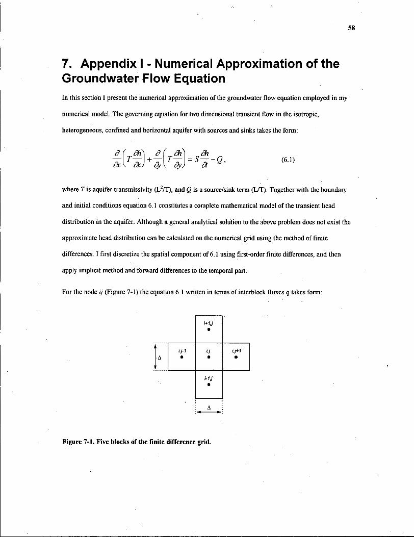
58

7. Appendix I - Numerical Approximation of the Groundwater Flow Equation In this section I present the numerical approximation of the groundwater flow equation employed in my

numerical model. The governing equation for two dimensional transient flow in the isotropic,

heterogeneous, confined and horizontal aquifer with sources and sinks takes the form:

~r [T— \+— T— =S—-Q, (6.1) ck\ ac) dy\ dy) a

where T is aquifer transmissivity (L2/T), and Q is a source/sink term (L/T). Together with the boundary

and initial conditions equation 6.1 constitutes a complete mathematical model of the transient head

distribution in the aquifer. Although a general analytical solution to the above problem does not exist the

approximate head distribution can be calculated on the numerical grid using the method of finite

differences. I first discretize the spatial component of 6.1 using first-order finite differences, and then

apply implicit method and forward differences to the temporal part.

For the node ij (Figure 7-1) the equation 6.1 written in terms of interblock fluxes q takes form:

i+1J •

A ij-1 • U • •

i-1J •

A

Figure 7-1. Five blocks of the finite difference grid.

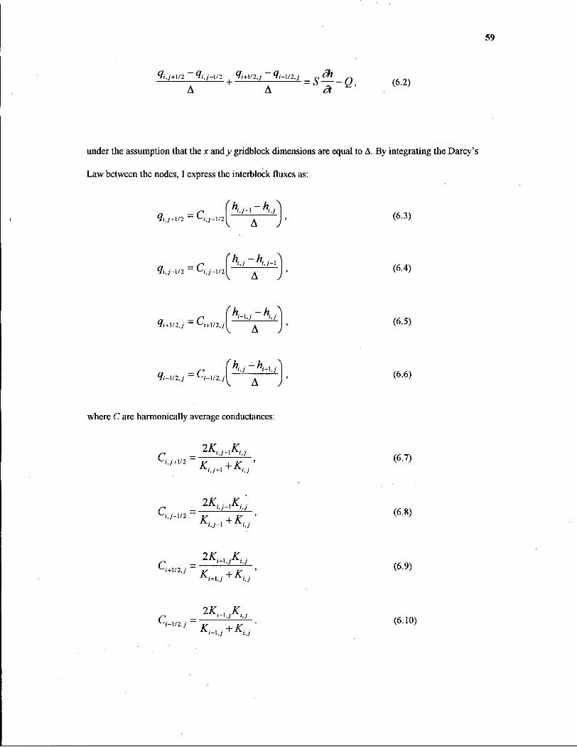
59

A + A = s ~ a ' Q ' . ( 6 2 )

under the assumption that the x andy gridblock dimensions are equal to A. By integrating the Darcy's

Law between the nodes, I express the interblock fluxes as:

A J (6.3)

(7i,;'-l/2 ~ Ci,j-\I2 I A J (6.4)

ai+\/2J ~ Q+l/2.;'

rh -h \ "i+U "i.j

A J (6.5)

ai-M2.j (h -h ^ 1 "i.j "i-\.j 1-1/2,;' ^ A ;

(6.6)

where C are harmonically average conductances:

c . ,;'+i/2

2Ki.j+\Ki,j

Ki.j+\ + Ki,j (6.7)

c ^i'.;'-l/2 .

2 ^ ; A , (6.8)

i+1/2,;'

2K<+,AJ K„,J + K,J

(6.9)

1-1/2,;'

2 * - . A ; (6.10)

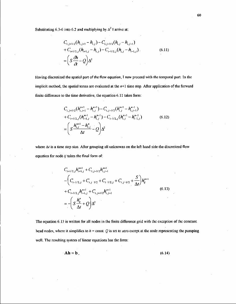
60

Substituting 6.3-6 into 6.2 and multiplying by A21 arrive at:

Q .y + i/2(A , , + i " Kj)~ Cu-m{Kj ~ Kj-\)

+ CMI2J(hMJ - hu)- C,_ 1 / 2 > ; (//,,. - h,_u)

v a )

(6.11)

Having discretized the spatial part of the flow equation, I now proceed with the temporal part. In the

implicit method, the spatial terms are evaluated at the n+l time step. After application of the forward

finite difference to the time derivative, the equation 6.11 takes form:

c , , + 1 / a ( C . - ^ ' ) - c , / . 1 / J ( ^ , - / C - . )

+cmjv&t - K?) - c^QC - O At Q

(6.12)

where At is a time step size. After grouping all unknowns on the left hand side the discretized flow

equation for node y takes the final form of:

*-i+l/2,/'i+lj T n+l

r n+l

At)

^ ^i-U2,j"i-\,j T S ' , y + l / 2 " / , ; + l

At

(6.13)

The equation 6.13 is written for all nodes in the finite difference grid with the exception of the constant

head nodes, where it simplifies to h = const. Q is set to zero except at the node representing the pumping

well. The resulting system of linear equations has the form:

Ah = b, (6.14)

61

where A is the penta-diagonal matrix of coefficients on the left hand side of 6.13, h is the hydraulic head

vector at n+l time step, and b is known right hand side vector. I use successive over-relaxation (SOR)

algorithm (Press et al. 1989) to solve 6.14.

Equation 6.14 provides hydraulic head solution for one time step. However my simulations require

calculations of head changes over several time steps. Therefore 6.14 has to be solved repeatedly until I

reach a desired length of simulation. I discretize time following suggestions of Anderson and Woessner

(1992). The initial time step Ar,„„ is set to value smaller then

SA2

to minimize head oscillations at the early times. The successive time steps are increased by a factor of V2.

Both sensitivity analysis of Section 2.4.3 and Monte Carlo runs in Sections 4.2 and 4.3 require repetitive

use of the flow simulator. Because the analysis is computer intensive, it is important to avoid redundant

calculations to shorten time of analysis. Therefore I optimize my code based on the close examination of

6.13 and 6.14.1 observe that only diagonal of matrix A and right hand side vector b change during time

stepping. Consequently at each time step I update only the diagonal of A and vector b, and avoid

recalculations of off-diagonal coefficients of A. This approach is different from procedures used in

standard groundwater simulators.

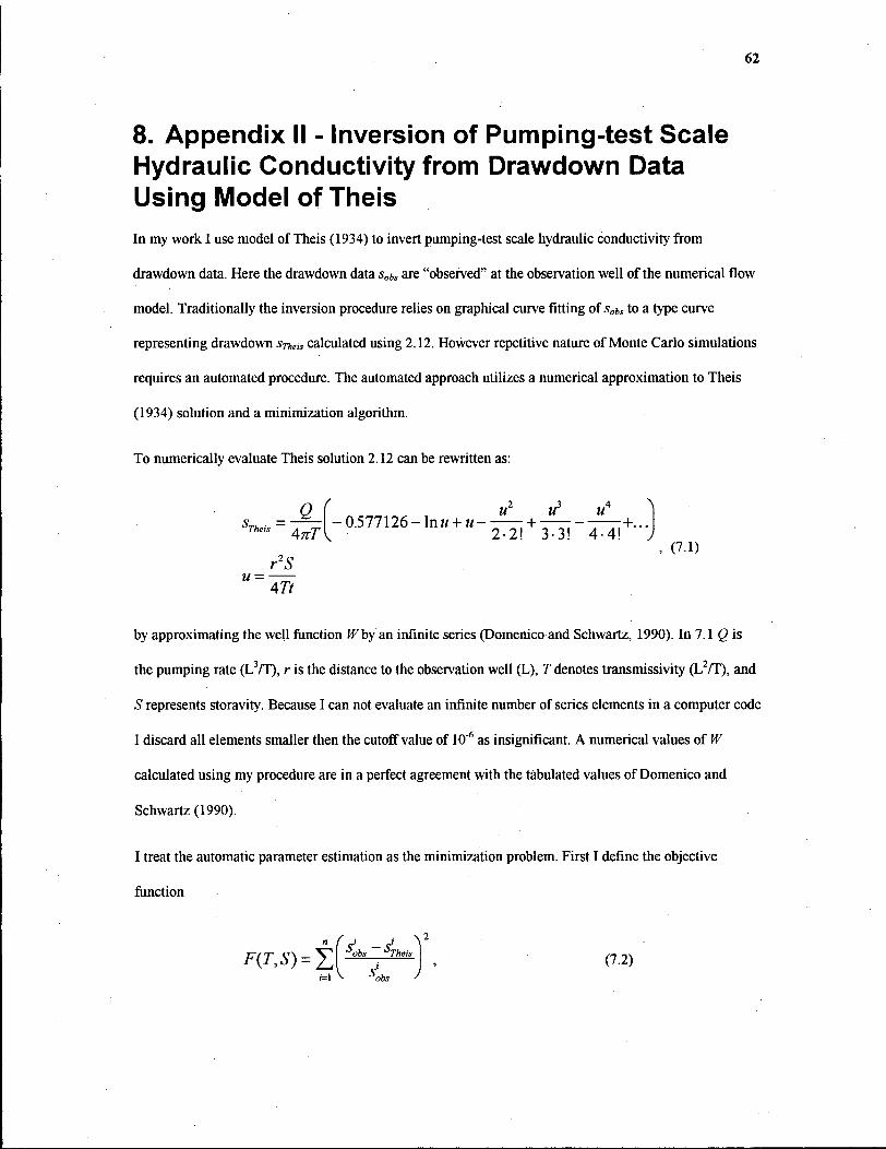
62

8. A p p e n d i x II - Inversion of Pumping- tes t S c a l e Hydraul ic Conduct iv i ty from D r a w d o w n Data U s i n g M o d e l of Theis In my work I use model of Theis (1934) to invert pumping-test scale hydraulic conductivity from

drawdown data. Here the drawdown data sobs are "observed" at the observation well of the numerical flow

model. Traditionally the inversion procedure relies on graphical curve fitting of sobs to a type curve

representing drawdown smis calculated using 2.12. However repetitive nature of Monte Carlo simulations

requires an automated procedure. The automated approach utilizes a numerical approximation to Theis

(1934) solution and a minimization algorithm.

To numerically evaluate Theis solution 2.12 can be rewritten as:

Q f ..2 ..2 „.4

STheis It u u

0.577126- In u + u- + -+... 2-2! 3-3! 4-4!

' , (7.1) r2S

u = —— 477

by approximating the well function ff by an infinite series QDomenico and Schwartz, 1990). In 7.1 Q is

the pumping rate (L?/T), r is the distance to the observation well (L), T denotes transmissivity (L2fT), and

S represents storavity. Because I can not evaluate an infinite number of series elements in a computer code

I discard all elements smaller then the cutoff value of 10s as insignificant. A numerical values of W

calculated using my procedure are in a perfect agreement with the tabulated values of Domenico and

Schwartz (1990).

I treat the automatic parameter estimation as the minimization problem. First I define the objective

function

F(T,S) = Z - 5 ' V

(7.2) obs

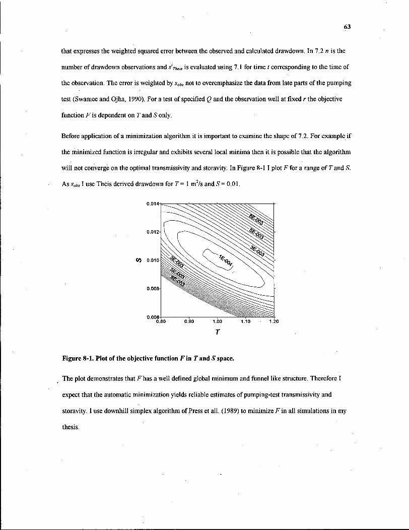
63

that expresses the weighted squared error between the observed and calculated drawdown. In 7.2 n is the

number of drawdown observations and s'-n^ is evaluated using 7.1 for time t corresponding to the time of

the observation. The error is weighted by sobs not to overemphasize the data from late parts of the pumping

test (Swamee and Ojha, 1990). For a test of specified Q and the observation well at fixed r the objective

function F is dependent on T and S only.

Before application of a minimization algorithm it is important to examine the shape of 7.2. For example if

the minimized function is irregular and exhibits several local minima then it is possible that the algorithm

will not converge on the optimal transmissivity and storavity. In Figure 8-11 plot F for a range of T and S.

As sobs I use Theis derived drawdown for T = 1 m2/s and S = 0.01.

Figure 8-1. Plot of the objective function F in T and S space.

The plot demonstrates that F has a well defined global minimum and funnel like structure. Therefore I

expect that the automatic minimization yields reliable estimates of pumping-test transmissivity and

storavity. I use downhill simplex algorithm of Press et all. (1989) to minimize F in all simulations in my

thesis.

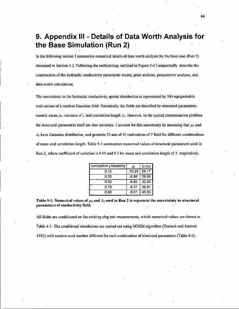
64

9. A p p e n d i x III - Details of Data Worth A n a l y s i s for the B a s e S imulat ion (Run 2) In the following section I summarize numerical details of data worth analysis for the base case (Run 2)

discussed in Section 4.2. Following the methodology outlined in Figure 3-2 I sequentially describe the

construction of the hydraulic conductivity uncertainty model, prior analysis, preposterior analysis, and

data worth calculations.

The uncertainty in the hydraulic conductivity spatial distribution is represented by 500 equiprobable

realizations of a random Gaussian field. Statistically the fields are described by structural parameters,

namely mean juY, variance cfY, and correlation length XY. However, in the typical contamination problem

the structural parameters itself are also uncertain. I account for this uncertainty by assuming that nY and

XY have Gaussian distribution, and generate 25 sets of 20 realizations of 7 field for different combinations

of mean and correlation length. Table 9-1 summarizes numerical values of structural parameters used in

Run 2, where coefficient of variation is 0.05 and 0.2 for mean and correlation length of Y, respectively.

cumulative probability 2r(m) 0.10 -10.24 24.17 0.30 -9.88 29.09 0.50 -9.62 32.50 0.70 -9.37 35.91 0.90 -9.01 40.83

Table 9-1. Numerical values of nY and AY used in Run 2 to represent the uncertainty in structural parameters of conductivity field.

All fields are conditioned on the existing slug test measurements, which numerical values are shown in

Table 4-1. The conditional simulations are carried out using SGSIM algorithm (Deutsch and Journel,

1992) with random seed number different for each combination of structural parameters (Table 9-2).

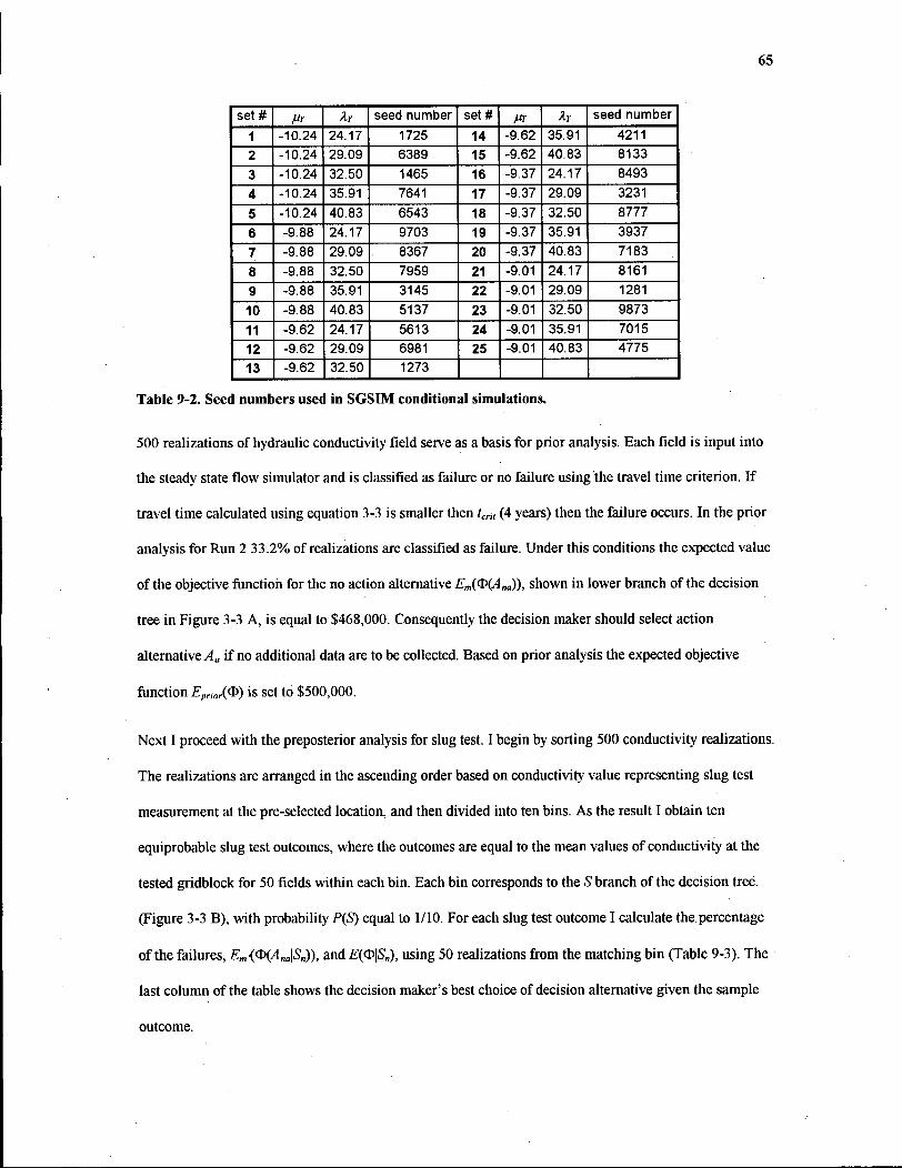
65

set# Mr Xy seed number set# Mr Xy seed number 1 -10.24 24.17 1725 14 -9.62 35.91 4211 2 -10.24 29.09 6389 15 -9.62 40.83 8133 3 -10.24 32.50 1465 16 -9.37 24.17 8493 4 -10.24 35.91 7641 17 -9.37 29.09 3231 5 -10.24 40.83 6543 18 -9.37 32.50 8777 6 -9.88 24.17 9703 19 -9.37 35.91 3937 7 -9.88 29.09 8367 20 -9.37 40.83 7183 8 -9.88 32.50 7959 21 -9.01 24.17 8161 9 -9.88 35.91 3145 22 -9.01 29.09 1281 10 -9.88 40.83 5137 23 -9.01 32.50 9873 11 -9.62 24.17 5613 24 -9.01 35.91 7015 12 -9.62 29.09 6981 25 -9.01 40.83 4775 13 -9.62 32.50 1273

Table 9-2. Seed numbers used in SGSIM conditional simulations.

500 realizations of hydraulic conductivity field serve as a basis for prior analysis. Each field is input into

the steady state flow simulator and is classified as failure or no failure using the travel time criterion. If

travel time calculated using equation 3-3 is smaller then tcrit (4 years) then the failure occurs. In the prior

analysis for Run 2 33.2% of realizations are classified as failure. Under this conditions the expected value

of the objective function for the no action alternative Em(Q>(A„a))y shown in lower branch of the decision

tree in Figure 3-3 A, is equal to $468,000. Consequently the decision maker should select action

alternative Aa if no additional data are to be collected. Based on prior analysis the expected objective

function Eprior(<&) is set to $500,000.

Next I proceed with the preposterior analysis for slug test. I begin by sorting 500 conductivity realizations.

The realizations are arranged in the ascending order based on conductivity value representing slug test

measurement at the pre-selected location, and then divided into ten bins. As the result I obtain ten

equiprobable slug test outcomes, where the outcomes are equal to the mean values of conductivity at the

tested gridblock for 50 fields within each bin. Each bin corresponds to the S branch of the decision tree.

(Figure 3-3 B), with probability P(S) equal to 1/10. For each slug test outcome I calculate the percentage

of the failures, Em{Q>(A„a\S„)), and E(Q)\S„), using 50 realizations from the matching bin (Table 9-3). The

last column of the table shows the decision maker's best choice of decision alternative given the sample

outcome.

66

bin # failure % Em{WA«*\Sn)) decision 1 06% $740,000 $740,000 no action 2 16 % $640,000 $640,000 no action 3 28 % $520,000 $520,000 no action 4 20% $600,000 $600,000 no action 5 40% $400,000 $500,000 action 6 34% $460,000 $500,000 action 7 28% $520,000 $520,000 no action 8 40% $400,000 $500,000 action 9 58 % $220,000 $500,000 action 10 62% $180,000 $500,000 action

Table 9-3. Details of slug-test preposterior analysis for Run 2.

The slug-test preposterior expected expected value of the objective function is calculated using equation

3.5, and is equal to $552,000. The data worth of slug test, being the difference between the preposterior

and prior objective function (equation 3.6), is equal to $52,000.

The preposterior analysis of pumping-test differs from the above by using pumping-test scale

conductivities as a sorting criterion. I sort the fields using pumping-test scale conductivity inverted from

the transient drawdown recorded for each realization. The numerical results for pumping-test with

observation well 8 meters away are shown below (Table 9-4).

bin # failure % Em«t>(A„JS„)) E«t>\S„) decision 1 06 % $740,000 $740,000 no action 2 08 % $720,000 $720,000 no action 3 14% $660,000 $660,000 no action 4 24% $560,000 $560,000 no action 5 24% $560,000 $560,000 no action 6 24% $560,000 $560,000 no action 7 44 % $360,000 $500,000 action 8 38 % $420,000 $500,000 action 9 68% $120,000 $500,000 action 10 82% $-20,000 $500,000 action

Table 9-4. Details of preposterior analysis for pumping test with observation well at 8 m, Run 2.

Error! Not a valid bookmark self-reference, presents preposterior expected expected values of the

objective function together with the corresponding data worth for pumping-test with distance to the

observation well equal to 4, 6, and 8 meters.

Distance to obs. well r (m) EJE<MS)) Worth 4 $568,000 $68,000 6 $574,000 $74,000 8 $579,000 $79,000

Table 9-5. Numerical results for pumping-test preposterior and data worth analysis for Run 2.