
Data Warehousing and Data Mining Unit 1 and 2 - diz Worlddizworld.com/dizyDownload/Unit 1-2...
21
Data Warehousing and Data Mining Unit 1 and 2 What is a Data Warehouse? Defined in many different ways, but not rigorously. A decision support database that is maintained separately from the organization’s operational database Support information processing by providing a solid platform of consolidated, historical data for analysis. “A data warehouse is a subject-oriented , integrated , time-variant , and nonvolatile collection of data in support of management’s decision-making process.”—W. H. Inmon Data warehousing: The process of constructing and using data warehouses Data Warehouse—Subject-Oriented Organized around major subjects, such as customer, product, sales Focusing on the modeling and analysis of data for decision makers, not on daily operations or transaction processing Provide a simple and concise view around particular subject issues by excluding data that are not useful in the decision support process Data Warehouse—Integrated Constructed by integrating multiple, heterogeneous data sources relational databases, flat files, on-line transaction records Data cleaning and data integration techniques are applied. Ensure consistency in naming conventions, encoding structures, attribute measures, etc. among different data sources E.g., Hotel price: currency, tax, breakfast covered, etc. When data is moved to the warehouse, it is converted. Data Warehouse—Time Variant The time horizon for the data warehouse is significantly longer than that of operational systems Operational database: current value data Data warehouse data: provide information from a historical perspective (e.g., past 5-10 years)
Transcript of Data Warehousing and Data Mining Unit 1 and 2 - diz Worlddizworld.com/dizyDownload/Unit 1-2...

Data Warehousing and Data Mining Unit 1 and 2
What is a Data Warehouse?
Defined in many different ways, but not rigorously.
A decision support database that is maintained separately from the organization’s
operational database
Support information processing by providing a solid platform of consolidated, historical
data for analysis.
“A data warehouse is a subject-oriented, integrated, time-variant, and nonvolatile collection of
data in support of management’s decision-making process.”—W. H. Inmon
Data warehousing:
The process of constructing and using data warehouses
Data Warehouse—Subject-Oriented
Organized around major subjects, such as customer, product, sales
Focusing on the modeling and analysis of data for decision makers, not on daily operations or
transaction processing
Provide a simple and concise view around particular subject issues by excluding data that are
not useful in the decision support process
Data Warehouse—Integrated
Constructed by integrating multiple, heterogeneous data sources
relational databases, flat files, on-line transaction records
Data cleaning and data integration techniques are applied.
Ensure consistency in naming conventions, encoding structures, attribute measures, etc.
among different data sources
E.g., Hotel price: currency, tax, breakfast covered, etc.
When data is moved to the warehouse, it is converted.
Data Warehouse—Time Variant
The time horizon for the data warehouse is significantly longer than that of operational systems
Operational database: current value data
Data warehouse data: provide information from a historical perspective (e.g., past 5-10
years)
Every key structure in the data warehouse
Contains an element of time, explicitly or implicitly
But the key of operational data may or may not contain “time element”
Data Warehouse—Nonvolatile
A physically separate store of data transformed from the operational environment
Operational update of data does not occur in the data warehouse environment
Does not require transaction processing, recovery, and concurrency control mechanisms
Requires only two operations in data accessing:
initial loading of data and access of data
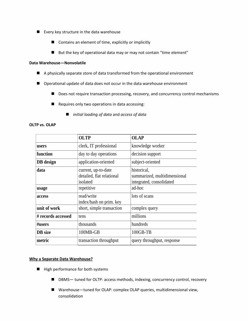
OLTP vs. OLAP
Why a Separate Data Warehouse?
High performance for both systems
DBMS— tuned for OLTP: access methods, indexing, concurrency control, recovery
Warehouse—tuned for OLAP: complex OLAP queries, multidimensional view,
consolidation
OLTP OLAP
users clerk, IT professional knowledge worker
function day to day operations decision support
DB design application-oriented subject-oriented
data current, up-to-date
detailed, flat relational
isolated
historical,
summarized, multidimensional
integrated, consolidated
usage repetitive ad-hoc
access read/write
index/hash on prim. key
lots of scans
unit of work short, simple transaction complex query
# records accessed tens millions
#users thousands hundreds
DB size 100MB-GB 100GB-TB
metric transaction throughput query throughput, response
Different functions and different data:
missing data: Decision support requires historical data which operational DBs do not
typically maintain
data consolidation: DS requires consolidation (aggregation, summarization) of data
from heterogeneous sources
data quality: different sources typically use inconsistent data representations, codes and
formats which have to be reconciled
Note: There are more and more systems which perform OLAP analysis directly on relational
databases
Three Data Warehouse Models
Enterprise warehouse
collects all of the information about subjects spanning the entire organization
Data Mart
a subset of corporate-wide data that is of value to a specific groups of users. Its scope is
confined to specific, selected groups, such as marketing data mart
Independent vs. dependent (directly from warehouse) data mart
Virtual warehouse
A set of views over operational databases
Only some of the possible summary views may be materialized
Extraction, Transformation, and Loading (ETL)
Data extraction
get data from multiple, heterogeneous, and external sources
Data cleaning
detect errors in the data and rectify them when possible
Data transformation
convert data from legacy or host format to warehouse format
Load
sort, summarize, consolidate, compute views, check integrity, and build indicies and
partitions
Refresh
propagate the updates from the data sources to the warehouse
From Tables and Spreadsheets to Data Cubes
A data warehouse is based on a multidimensional data model which views data in the form of a
data cube
A data cube, such as sales, allows data to be modeled and viewed in multiple dimensions
Dimension tables, such as item (item_name, brand, type), or time(day, week, month,
quarter, year)
Fact table contains measures (such as dollars_sold) and keys to each of the related
dimension tables
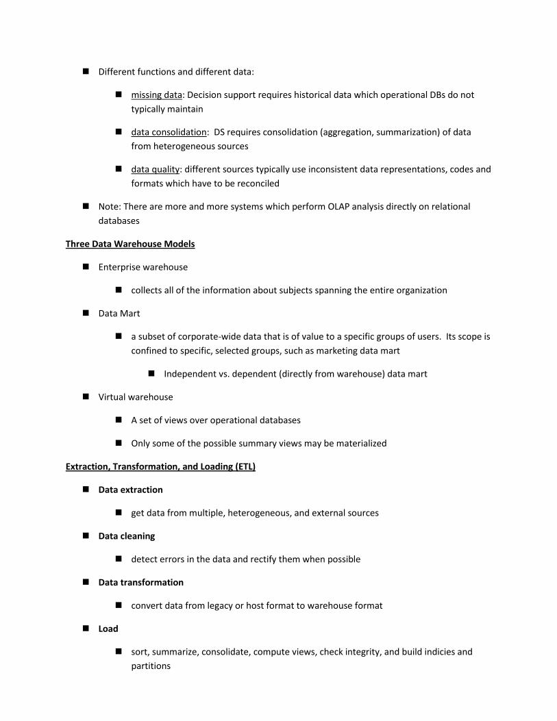
In data warehousing literature, an n-D base cube is called a base cuboid. The top most 0-D
cuboid, which holds the highest-level of summarization, is called the apex cuboid. The lattice of
cuboids forms a data cube.
Cube: A Lattice of Cuboids
Conceptual Modeling of Data Warehouses
Modeling data warehouses: dimensions & measures
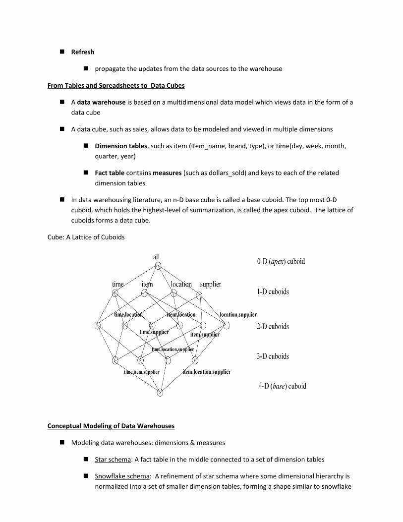
Star schema: A fact table in the middle connected to a set of dimension tables
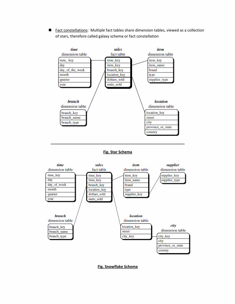
Snowflake schema: A refinement of star schema where some dimensional hierarchy is
normalized into a set of smaller dimension tables, forming a shape similar to snowflake
Fact constellations: Multiple fact tables share dimension tables, viewed as a collection
of stars, therefore called galaxy schema or fact constellation
Fig. Star Schema
Fig. Snowflake Schema
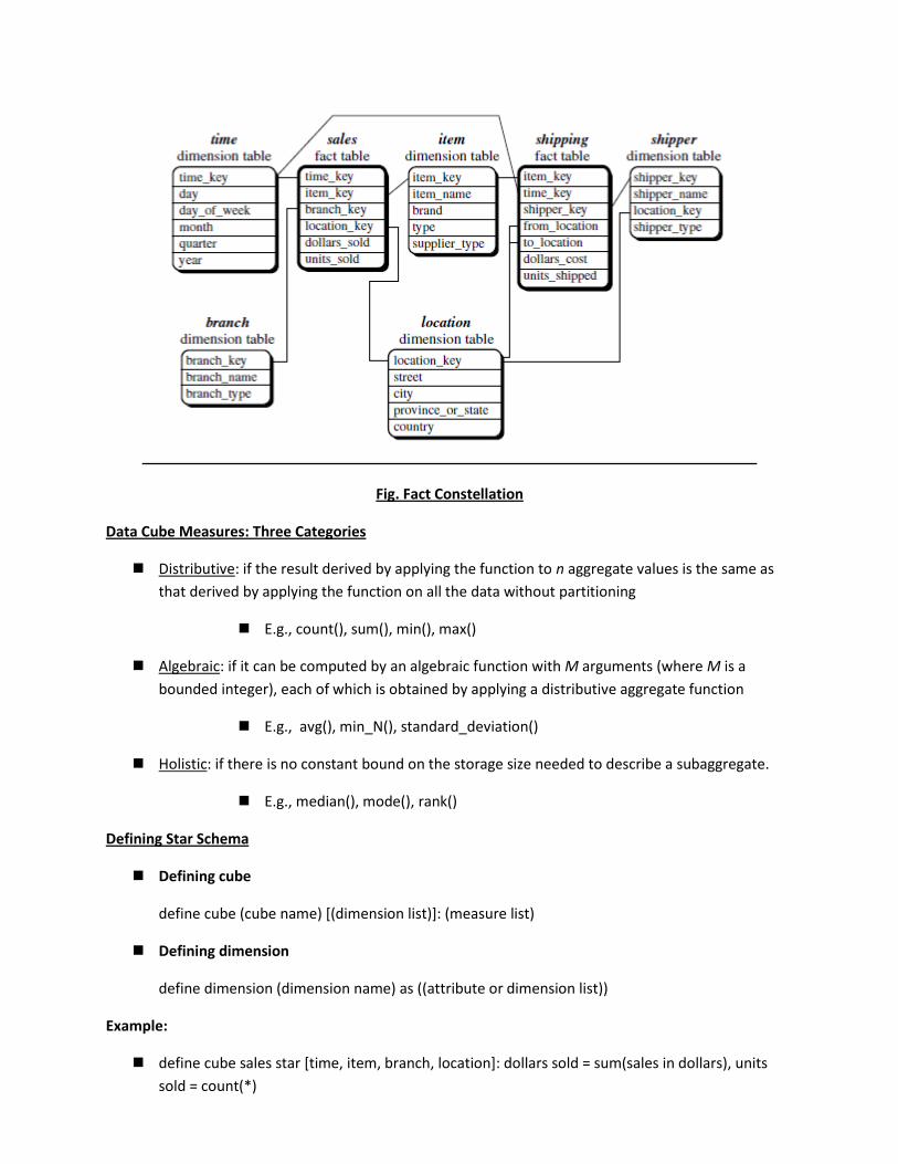
Fig. Fact Constellation
Data Cube Measures: Three Categories
Distributive: if the result derived by applying the function to n aggregate values is the same as
that derived by applying the function on all the data without partitioning
E.g., count(), sum(), min(), max()
Algebraic: if it can be computed by an algebraic function with M arguments (where M is a
bounded integer), each of which is obtained by applying a distributive aggregate function
E.g., avg(), min_N(), standard_deviation()
Holistic: if there is no constant bound on the storage size needed to describe a subaggregate.
E.g., median(), mode(), rank()
Defining Star Schema
Defining cube
define cube (cube name) [(dimension list)]: (measure list)
Defining dimension
define dimension (dimension name) as ((attribute or dimension list))
Example:
define cube sales star [time, item, branch, location]: dollars sold = sum(sales in dollars), units
sold = count(*)

define dimension time as (time key, day, day of week, month, quarter, year)
define dimension item as (item key, item name, brand, type, supplier type)
Defining Snowflake Schema
define cube sales snowflake [time, item, branch, location]:dollars sold = sum(sales in dollars),
units sold = count(*)
define dimension time as (time key, day, day of week, month, quarter, year)
define dimension item as (item key, item name, brand, type, supplier (supplier key, supplier
type))
define dimension branch as (branch key, branch name, branch type)
define dimension location as (location key, street, city (city key, city, province or state, country))
Defining fact constellation schema
define cube sales [time, item, branch, location]:
dollars sold = sum(sales in dollars), units sold = count(*)
define dimension time as (time key, day, day of week, month, quarter, year)
define dimension item as (item key, item name, brand, type, supplier type)
define dimension branch as (branch key, branch name, branch type)
define dimension location as (location key, street, city, province or state, country)
define cube shipping [time, item, shipper, from location, to location]:dollars cost = sum(cost in
dollars), units shipped = count(*)
define dimension time as time in cube sales
define dimension item as item in cube sales
define dimension shipper as (shipper key, shipper name, location as location in cube sales,
shipper type)
define dimension from location as location in cube sales
define dimension to location as location in cube sales
Data Cube Measures: Three Categories
A data cube measure is a numerical function that can be evaluated
at each point in the data cube space.
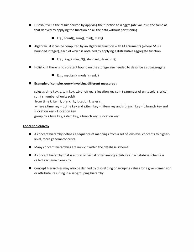
Distributive: if the result derived by applying the function to n aggregate values is the same as
that derived by applying the function on all the data without partitioning
E.g., count(), sum(), min(), max()
Algebraic: if it can be computed by an algebraic function with M arguments (where M is a
bounded integer), each of which is obtained by applying a distributive aggregate function
E.g., avg(), min_N(), standard_deviation()
Holistic: if there is no constant bound on the storage size needed to describe a subaggregate.
E.g., median(), mode(), rank()
Example of complex query involving different measures :
select s.time key, s.item key, s.branch key, s.location key,sum ( s.number of units sold s.price),
sum( s.number of units sold)
from time t, item i, branch b, location l, sales s,
where s.time key = t.time key and s.item key = i.item key and s.branch key = b.branch key and
s.location key = l.location key
group by s.time key, s.item key, s.branch key, s.location key
Concept hierarchy
A concept hierarchy defines a sequence of mappings from a set of low-level concepts to higher-
level, more general concepts.
Many concept hierarchies are implicit within the database schema.
A concept hierarchy that is a total or partial order among attributes in a database schema is
called a schema hierarchy.
Concept hierarchies may also be defined by discretizing or grouping values for a given dimension
or attribute, resulting in a set-grouping hierarchy.
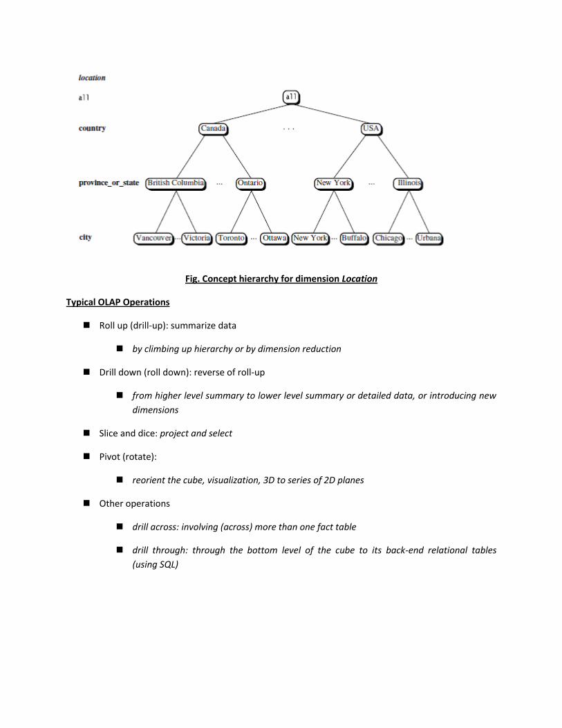
Fig. Concept hierarchy for dimension Location
Typical OLAP Operations
Roll up (drill-up): summarize data
by climbing up hierarchy or by dimension reduction
Drill down (roll down): reverse of roll-up
from higher level summary to lower level summary or detailed data, or introducing new
dimensions
Slice and dice: project and select
Pivot (rotate):
reorient the cube, visualization, 3D to series of 2D planes
Other operations
drill across: involving (across) more than one fact table
drill through: through the bottom level of the cube to its back-end relational tables
(using SQL)

Fig. Different OLAP Operations

Data Warehouse Usage
Three kinds of data warehouse applications
Information processing
supports querying, basic statistical analysis, and reporting using crosstabs,
tables, charts and graphs
Analytical processing
multidimensional analysis of data warehouse data
supports basic OLAP operations, slice-dice, drilling, pivoting
Data mining
knowledge discovery from hidden patterns
supports associations, constructing analytical models, performing classification
and prediction, and presenting the mining results using visualization tools
Design of Data Warehouse: A Business Analysis Framework
Gains for analyst
a. Competitive advantage c. Productivity
b. CRM d. Cost reduction
Four views regarding the design of a data warehouse
Top-down view
allows selection of the relevant information necessary for the data warehouse
Data source view
exposes the information being captured, stored, and managed by operational
systems
Data warehouse view
consists of fact tables and dimension tables
Business query view
sees the perspectives of data in the warehouse from the view of end-user
Data Warehouse Design Process
Top-down, bottom-up approaches or a combination of both

Top-down: Starts with overall design and planning (mature)
Bottom-up: Starts with experiments and prototypes (rapid)
From software engineering point of view
Planning, requirements study, problem analysis, warehouse design, data integration and testing,
and finally deployment of the data warehouse.
Waterfall: structured and systematic analysis at each step before proceeding to the next
Spiral: rapid generation of increasingly functional systems, short turn around time,
quick turn around
Typical data warehouse design process
Choose a business process to model, e.g., orders, invoices, etc.
Choose the grain (atomic level of data) of the business process
Choose the dimensions that will apply to each fact table record
Choose the measure that will populate each fact table record
Steps after data warehouse design
Initial deployment -initial installation, roll-out planning, training, and orientation. Platform
upgrade and maintenance
Data warehouse administration - data refreshment, data source synchronization, planning for
disaster recovery, managing access control and security, managing data growth, managing
database performance, and data warehouse enhancement and extension
Scope management - controlling the number and range of queries, dimensions, and reports;
limiting the size of the data warehouse; or limiting the schedule, budget, or resources.
A 3-tier Data Warehousing Architecture

Fig. A 3 – tier Data Warehouse Architecture
Three Data Warehouse Models
Enterprise warehouse
collects all of the information about subjects spanning the entire organization
Data Mart
a subset of corporate-wide data that is of value to a specific groups of users. Its scope is
confined to specific, selected groups, such as marketing data mart
Independent vs. dependent (directly from warehouse) data mart
Virtual warehouse
A set of views over operational databases
Only some of the possible summary views may be materialized
Data Warehouse Back-End Tools and Utilities
Data Warehouse Back-End Tools and Utilities includes the following functions
Data extraction
get data from multiple, heterogeneous, and external sources
Data cleaning
detect errors in the data and rectify them when possible
Data transformation
convert data from legacy or host format to warehouse format
Load
sort, summarize, consolidate, compute views, check integrity, and build indices and
partitions
Refresh
propagate the updates from the data sources to the warehouse
Besides these, data warehouse systems usually provide a good set of data warehouse
management tools.
Metadata Repository
Meta data is the data defining warehouse objects. It stores:
Description of the structure of the data warehouse
schema, view, dimensions, hierarchies, derived data defn, data mart locations and
contents
Operational meta-data
data lineage (history of migrated data and transformation path), currency of data
(active, archived, or purged), monitoring information (warehouse usage statistics, error
reports, audit trails)
The algorithms used for summarization
The mapping from operational environment to the data warehouse
Data related to system performance
warehouse schema, view and derived data definitions
Business data
business terms and definitions, ownership of data, charging policies
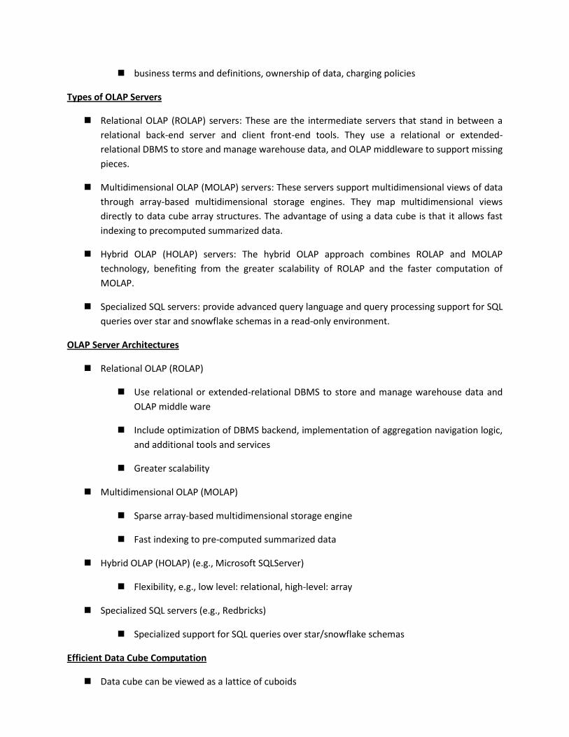
Types of OLAP Servers
Relational OLAP (ROLAP) servers: These are the intermediate servers that stand in between a
relational back-end server and client front-end tools. They use a relational or extended-
relational DBMS to store and manage warehouse data, and OLAP middleware to support missing
pieces.
Multidimensional OLAP (MOLAP) servers: These servers support multidimensional views of data
through array-based multidimensional storage engines. They map multidimensional views
directly to data cube array structures. The advantage of using a data cube is that it allows fast
indexing to precomputed summarized data.
Hybrid OLAP (HOLAP) servers: The hybrid OLAP approach combines ROLAP and MOLAP
technology, benefiting from the greater scalability of ROLAP and the faster computation of
MOLAP.
Specialized SQL servers: provide advanced query language and query processing support for SQL
queries over star and snowflake schemas in a read-only environment.
OLAP Server Architectures
Relational OLAP (ROLAP)
Use relational or extended-relational DBMS to store and manage warehouse data and
OLAP middle ware
Include optimization of DBMS backend, implementation of aggregation navigation logic,
and additional tools and services
Greater scalability
Multidimensional OLAP (MOLAP)
Sparse array-based multidimensional storage engine
Fast indexing to pre-computed summarized data
Hybrid OLAP (HOLAP) (e.g., Microsoft SQLServer)
Flexibility, e.g., low level: relational, high-level: array
Specialized SQL servers (e.g., Redbricks)
Specialized support for SQL queries over star/snowflake schemas
Efficient Data Cube Computation
Data cube can be viewed as a lattice of cuboids

The bottom-most cuboid is the base cuboid
The top-most cuboid (apex) contains only one cell
How many cuboids in an n-dimensional cube with L levels?
Materialization of data cube
Materialize every (cuboid) (full materialization), none (no materialization), or
some (partial materialization)
Selection of which cuboids to materialize
Based on size, sharing, access frequency, etc.
The “Compute Cube” Operator
Cube definition and computation in DMQL
define cube sales [item, city, year]: sum (sales_in_dollars)
compute cube sales
Transform it into a SQL-like language (with a new operator cube by, introduced by Gray et al.’96)
SELECT item, city, year, SUM (amount) FROM SALES CUBE BY item, city, year
Need compute the following Group-Bys
(date, product, customer),
(date,product),(date, customer), (product, customer),
(date), (product), (customer)
()
)11(
n
ii
LT

Partial Materialization: Selected Computation of Cuboids
There are three choices for data cube materialization given a base cuboid:
1. No materialization: Do not precompute any of the “nonbase” cuboids.
2. Full materialization: Precompute all of the cuboids. The resulting lattice of computed cuboids
is referred to as the full cube.
3. Partial materialization: Selectively compute a proper subset of the whole set of possible
cuboids.
The partial materialization of cuboids or subcubes should consider three factors:
(1) identify the subset of cuboids or subcubes to materialize;
(2) exploit the materialized cuboids or subcubes during query processing;
(3) efficiently update the materialized cuboids or subcubes during load and refresh.
Indexing OLAP Data: Bitmap Index
Index on a particular column
Each value in the column has a bit vector: bit-op is fast
The length of the bit vector: # of records in the base table
The i-th bit is set if the i-th row of the base table has the value for the indexed column
not suitable for high cardinality domains
A recent bit compression technique, Word-Aligned Hybrid (WAH), makes it work for high
cardinality domain as well *Wu, et al. TODS’06+
Base Table Index on Register Index on Type
Indexing OLAP Data: Join Indices
Join index: JI(R-id, S-id) where R (R-id, …) S (S-id, …)
Traditional indices map the values to a list of record ids
Cust Region Type
C1 Asia Retail
C2 Europe Dealer
C3 Asia Dealer
C4 America Retail
C5 Europe Dealer
RecID Retail Dealer
1 1 0
2 0 1
3 0 1
4 1 0
5 0 1
RecIDAsia Europe America
1 1 0 0
2 0 1 0
3 1 0 0
4 0 0 1
5 0 1 0

It materializes relational join in JI file and speeds up relational join
In data warehouses, join index relates the values of the dimensions of a start schema to rows in
the fact table.
E.g. fact table: Sales and two dimensions city and product
A join index on city maintains for each distinct city a list of R-IDs of the tuples
recording the Sales in the city
Join indices can span multiple dimensions
Efficient Processing OLAP Queries
Determine which operations should be performed on the available cuboids
Transform drill, roll, etc. into corresponding SQL and/or OLAP operations, e.g., dice =
selection + projection
Determine which materialized cuboid(s) should be selected for OLAP op.
Let the query to be processed be on {brand, province_or_state} with the condition “year
= 2004”, and there are 4 materialized cuboids available:
1) {year, item_name, city}
2) {year, brand, country}
3) {year, brand, province_or_state}

4) {item_name, province_or_state} where year = 2004
Which should be selected to process the query?
Explore indexing structures and compressed vs. dense array structs in MOLAP
Further Development of Data Cube and OLAP Technology
Section 1 describes data mining by discovery-driven exploration of data cubes, where anomalies
in the data are automatically detected and marked for the user with visual cues.
Section 2 describes multifeature cubes for complex data mining queries involving multiple
dependent aggregates at multiple granularity.
Section 3 presents methods for constrained gradient analysis in data cubes, which identifies
cube cells that have dramatic changes in value in comparison with their siblings, ancestors, or
descendants.
Discovery-Driven Exploration of Data Cubes
Hypothesis-driven
exploration by user, huge search space
Discovery-driven (Sarawagi, et al.’98)
Effective navigation of large OLAP data cubes
pre-compute measures indicating exceptions, guide user in the data analysis, at all levels
of aggregation
Exception: significantly different from the value anticipated, based on a statistical model
Visual cues such as background color are used to reflect the degree of exception of each
cell
Kinds of Exceptions and their Computation
Parameters
SelfExp: surprise of cell relative to other cells at same level of aggregation
InExp: surprise beneath the cell
PathExp: surprise beneath cell for each drill-down path
Computation of exception indicator (modeling fitting and computing SelfExp, InExp, and PathExp
values) can be overlapped with cube construction
Exception themselves can be stored, indexed and retrieved like precomputed aggregates
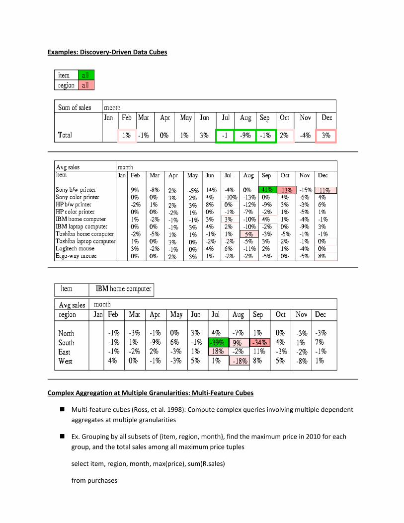
Examples: Discovery-Driven Data Cubes
Complex Aggregation at Multiple Granularities: Multi-Feature Cubes
Multi-feature cubes (Ross, et al. 1998): Compute complex queries involving multiple dependent
aggregates at multiple granularities
Ex. Grouping by all subsets of {item, region, month}, find the maximum price in 2010 for each
group, and the total sales among all maximum price tuples
select item, region, month, max(price), sum(R.sales)
from purchases
where year = 2010
cube by item, region, month: R
such that R.price = max(price)
Continuing the last example, among the max price tuples, find the min and max shelf live, and
find the fraction of the total sales due to tuple that have min shelf life within the set of all max
price tuples
Constrained Gradient Analysis in Data Cubes
The problem of mining changes of complex measures in a multidimensional space is the
cubegrade problem, which can be viewed as a generalization of association rules and data
cubes.
It studies how changes in a set of measures (aggregates) of interest are associated with changes
in the underlying characteristics of sectors, where changes in sector characteristics are
expressed in terms of dimensions of the cube and are limited to specialization (drilldown),
generalization (roll-up), and mutation (a change in one of the cube’s dimensions).
The cubegrade problem is significantly more expressive than association rules.
Constrained multidimensional gradient analysis, which reduces the search space and derives
interesting results.
It incorporates the following types of constraints:
I. Significance constraint - This ensures that we examine only the cells that have certain
“statistical significance” in the data.
II. Probe constraint - This selects a subset of cells (called probe cells) from all of the possible cells
as starting points for examination.
III. Gradient constraint - This specifies the user’s range of interest on the gradient (measure
change).
A suggested method to compute gradients is a set oriented approach that starts with a set of
probe cells, utilizes constraints early on during search, and explores pruning, when possible,
during progressive computation of pairs of cells.
With each gradient cell, the set of all possible probe cells that might co-occur in interesting
gradient-probe pairs are associated with some descendants of the gradient cell. These probe
cells are considered “live probe cells.”
This set is used to search for future gradient cells, while considering significance constraints and
gradient constraints to reduce the search space.
The constrained cube gradient analysis has been shown to be effective at exploring the
significant changes among related cube cells in multidimensional space.


![Data Warehousing and Data Mining Notes [Unit i and II]](https://static.fdocuments.in/doc/165x107/553cf05255034657228b4b83/data-warehousing-and-data-mining-notes-unit-i-and-ii.jpg)