Data Structures -...

Data Structures

September 29

1

2

Org Remarks

• Send your Assignments (of course, zipped – since your work will usually consist of several files) to Simon Zaaijer (email: [email protected])

• In addition to the above turn in a paper copy of your work in class on the day of the deadline

• Let your zip file have a name which can be traced to your team in the following standard way – username1andUsername2No1.zip, – where username1 is the liacs username of the first member and

username2 is the liacs username of the second member

• Moreover: each file you are turning in should contain the names of the team members, date turned in, due date, Assignment No; all this in a conspicuous manner at the top of the files

• furthermore a README file should describe which files your turning in and instructions for compilation and execution, if necessary

2

Hierachical structures: Trees

•

3

4

Objectives

Discuss the following topics:

• Trees, Binary Trees, and Binary Search Trees

• Implementing Binary Trees

• Tree Traversal

• Searching a Binary Search Tree

• Insertion

• Deletion

5

Objectives (continued)

Discuss the following topics:

• Heaps

• Balancing a Tree

• Self-Adjusting Trees

6

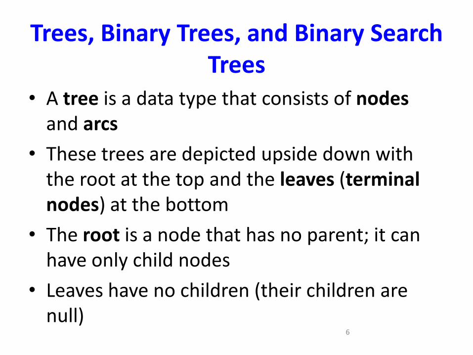
Trees, Binary Trees, and Binary Search Trees

• A tree is a data type that consists of nodesand arcs

• These trees are depicted upside down with the root at the top and the leaves (terminal nodes) at the bottom

• The root is a node that has no parent; it can have only child nodes

• Leaves have no children (their children are null)

7

Trees, Binary Trees, and Binary Search Trees (continued)

• Each node has to be reachable from the root through a unique sequence of arcs, called a path

• The number of arcs in a path is called the length of the path

• The level of a node is the length of the path from the root to the node plus 1, which is the number of nodes in the path

• The height of a nonempty tree is the maximum level of a node in the tree

8


Figure 6-1 Examples of trees

9


Figure 6-2 Hierarchical structure of a university shown as a tree

Trees (adt)

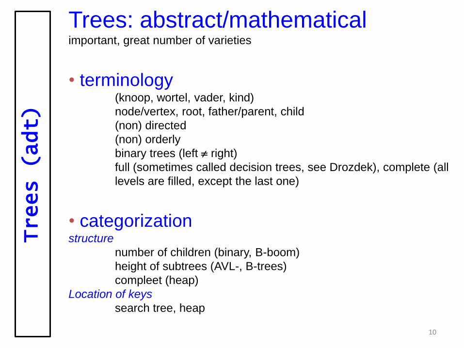
Trees: abstract/mathematicalimportant, great number of varieties

• terminology(knoop, wortel, vader, kind)

node/vertex, root, father/parent, child

(non) directed

(non) orderly

binary trees (left right)

full (sometimes called decision trees, see Drozdek), complete (all

levels are filled, except the last one)

• categorization structure

number of children (binary, B-boom)

height of subtrees (AVL-, B-trees)

compleet (heap)

Location of keys

search tree, heap

10

BOMEN

^

¬

v

ζ1

ζ3ζ2

expression code

A

D

CB

1

1

1

0

0

0

bst

trie

16

5 6 2

12

10

7

4 2heap

syntax

sat tues

fri mon

sun thurwed

B-tree (2,3 tree)

expr

term

term

term

expr*

fact

a

*fact

a

b

fact

thur

fri sat wed

tues

sun

mon

sc

a a e

a etr t

kl

11

Recall Definition of tree

1. An empty structure is a tree

2. If t1, ..., tk are trees, the structure whose root is a tree has as its children the roots of t1,...,tk is also a tree

3. Only structures generated by rule 1 and 2 are trees

Alternatively: a connected graph which contains no cycles(circuits) is a tree

12

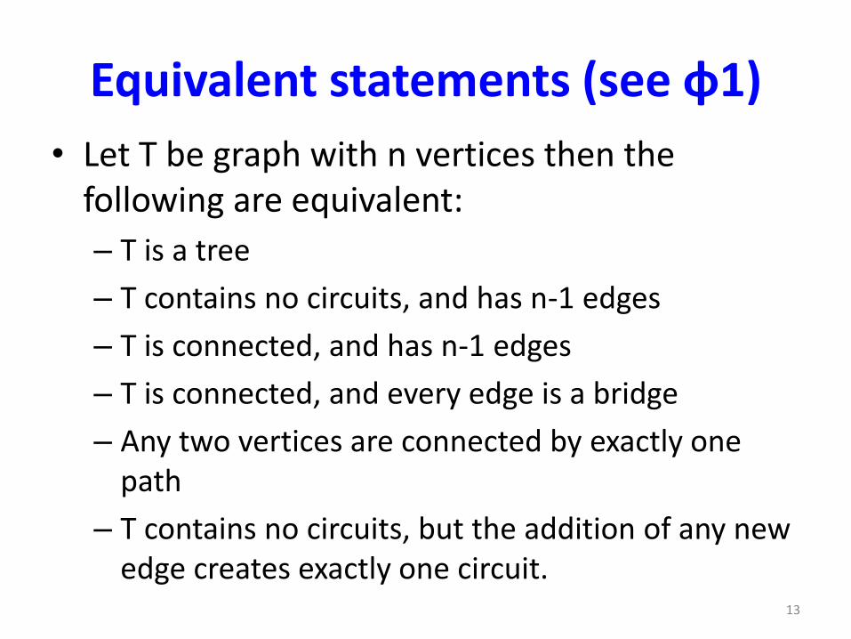
Equivalent statements (see φ1)

• Let T be graph with n vertices then the following are equivalent:

– T is a tree

– T contains no circuits, and has n-1 edges

– T is connected, and has n-1 edges

– T is connected, and every edge is a bridge

– Any two vertices are connected by exactly one path

– T contains no circuits, but the addition of any new edge creates exactly one circuit.

13

14


• An orderly tree is where all elements are stored according to some predetermined criterion of ordering

Figure 6-3 Transforming (a) a linked list into (b) a tree

15

Binary Trees

• A binary tree is a tree whose nodes have two children (possibly empty), and each child is designated as either a left child or a right child

Figure 6-4 Examples of binary trees

16

Binary Trees

• In a complete binary tree, all the nodes at all levels have two children except the last level.

• A decision tree is a binary tree in which all nodes have either zero or two nonempty children

Complete

Binary tree

Dutch: compleet)

Decision tree

(Dutch: vol)

complete

Decision treeincomplete

Binary tree

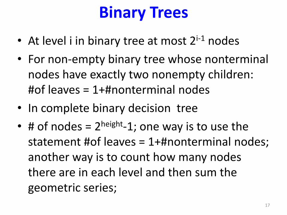
Binary Trees

• At level i in binary tree at most 2i-1 nodes

• For non-empty binary tree whose nonterminal nodes have exactly two nonempty children: #of leaves = 1+#nonterminal nodes

• In complete binary decision tree

• # of nodes = 2height-1; one way is to use the statement #of leaves = 1+#nonterminal nodes; another way is to count how many nodes there are in each level and then sum the geometric series;

17

18

Binary Trees

Figure 6-5 Adding a leaf to tree (a), preserving the relation of the

number of leaves to the number of nonterminal nodes (b)

ADT Binary Tree (more explicitly)createBinaryTree() //creates an empty binary tree

createBinary(rootItem) // creates a one-node bin tree whose root contains rootItem

createBinary(rootItem, leftTree, rightTree) //creates a bin tree whose root contains rootItem //and has leftTree and rightTree, respectively, as its left and right subtrees

destroyBinaryTree() // destroys a binary tree

rootData() // returns the data portion of the root of a nonempty binary tree

setRootData(newItem) // replaces the the data portion of the root of a //nonempty bin tree with newItem. If the bin tree is empty, however, //creates a root node whose data portion is newItem and inserts the new //node into the tree

attachLeft(newItem, success) // attaches a left child containing newItem to //the root of a binary tree. Success indicates whether the operation was //successful.

attachRight(newItem, success) // ananlogous to attachLeft19

ADT Binary Tree (continued)

attachLeftSubtree(leftTree, success) // Attaches leftTree as the left subtree to the root of a bin tree. Success indicates whether the operation was successful.

attachRightSubtree(rightTree, success) // analogous to attachLeftSubtree

detachLeftSubtree(leftTree, success) // detaches the left subtree of a bin tree’s root and retains it in leftTree. Success indicates whether the op was successful.

detachRightSubtree(rightTree, success) // similar to detachLeftSubtree

leftSubtree() // Returns, but does not detach, the left subtree of a bin tree’s root

rightSubtree() // analogous to leftSubtree

preorderTraverse(visit) // traverses a binary tree in preorder and calls the function visit once for each node

inorderTraverse(visit) // analogous: inorder

postorderTraverse(visit) // analogous: postorder

20

21

Implementing Binary Trees

• Binary trees can be implemented in at least two ways:

– As arrays

– As linked structures

• To implement a tree as an array, a node is declared as an object with an information field and two “reference” fields

22

Implementing Binary Trees (continued)

Figure 6-7 Array representation of the tree in Figure 6.6c

Can do for complete binary trees;

A[i] with children A[2i] and A[2i+1].

Parent of A[i] is A[i div 2].

0 8

root free

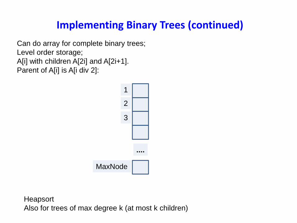
Implementing Binary Trees (continued)

Can do array for complete binary trees;

Level order storage;

A[i] with children A[2i] and A[2i+1].

Parent of A[i] is A[i div 2]:

(complete boom)

1

2

3

MaxNode

....

Heapsort

Also for trees of max degree k (at most k children)

Binary Tree C++

template <class T>

struct TreeNode {

T info;

TreeNode<T> *left, * right;

int tag // a.o. For threading

TreeNode ( const T& i,

TreeNode<T> *left = NULL,

TreeNode<T> *right = NULL )

: info(i)

{ left = l; right = r; tag = 0; }

};

constructor

of type T

default

constructor

template

See the next slide for the proof of concept; type T=int, is hardwired 24

The programmed ADT Binary Tree (refers to slide 20, 21: ADT Binary Tree)

not parametrized: itemType = int

// Client

// ADT

// Impl.

25

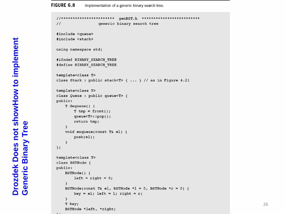
26

Dro

zd

ek

Do

es

no

t s

ho

wH

ow

to

im

ple

me

nt

Ge

ne

ric

Bin

ary

Tre

e

27

bst

28

bst

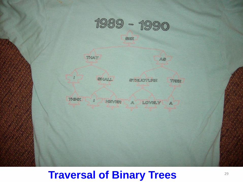
Traversal of Binary Trees 29

Traversal of Binary Trees 30

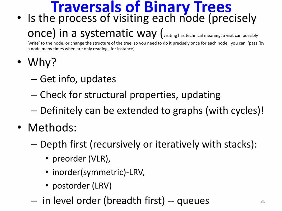
Traversals of Binary Trees• Is the process of visiting each node (precisely

once) in a systematic way (visiting has technical meaning, a visit can possibly

‘write’ to the node, or change the structure of the tree, so you need to do it precisely once for each node; you can ‘pass ‘bya node many times when are only reading , for instance)

• Why?

– Get info, updates

– Check for structural properties, updating

– Definitely can be extended to graphs (with cycles)!

• Methods:

– Depth first (recursively or iteratively with stacks):

• preorder (VLR),

• inorder(symmetric)-LRV,

• postorder (LRV)

– in level order (breadth first) -- queues 31

Traversals of Binary Trees

• Recursively

• Iteratively: stacks (Depth First)

• Queues for Breadth First

• Threaded Trees

• Tree Transformation (e.g., Morris)

32

33

Tree Traversal: breadth-first

• Breadth-first traversal is visiting each node starting from the lowest (or highest) level and moving down (or up) level by level, visiting nodes on each level from left to right (or from right to left)

34

Tree Traversal: breadth-first

3535

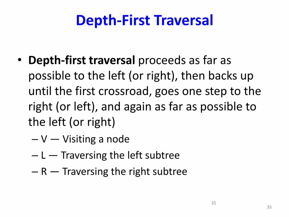
Depth-First Traversal

• Depth-first traversal proceeds as far as possible to the left (or right), then backs up until the first crossroad, goes one step to the right (or left), and again as far as possible to the left (or right)

– V — Visiting a node

– L — Traversing the left subtree

– R — Traversing the right subtree

36

Depth-First Traversal

37

Inorder Tree Traversal

Preorder Traversal – iterativeuses a stack

S.create();

S.push(root);

while (not S.isEmpty()) {

current = S.pop() // a retrieving pop

while (current ≠ NULL) {

visit(current);

S.push(current -> right);

current = current -> left

} // end while

} // end while 39

40

Preorder Traversal – iterative

41

Stackless Depth-First Traversal

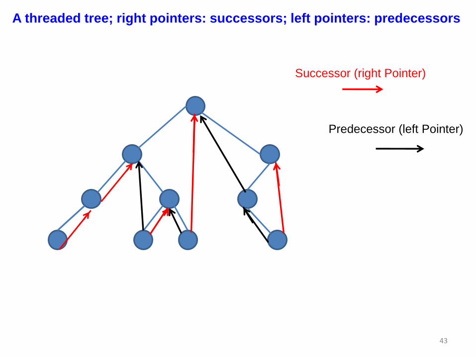
• Threads are references to the predecessor and successor of the node according to an inorder traversal

• Trees whose nodes use threads are called threaded trees

42

Successor (right Pointer)

A threaded tree; an inorder traversal´s path in a threaded tree with

Right successors only

43

Successor (right Pointer)

A threaded tree; right pointers: successors; left pointers: predecessors

Predecessor (left Pointer)

44

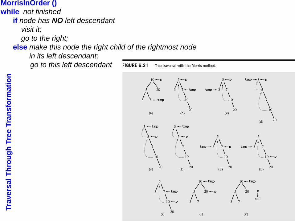
MorrisInOrder ()

while not finished

if node has NO left descendant

visit it;

go to the right;

else make this node the right child of the rightmost node

in its left descendant;

go to this left descendant

Tra

vers

al

Th

rou

gh

Tre

e T

ran

sfo

rmati

on

45Tra

vers

al

Th

rou

gh

Tre

e T

ran

sfo

rmati

on

46

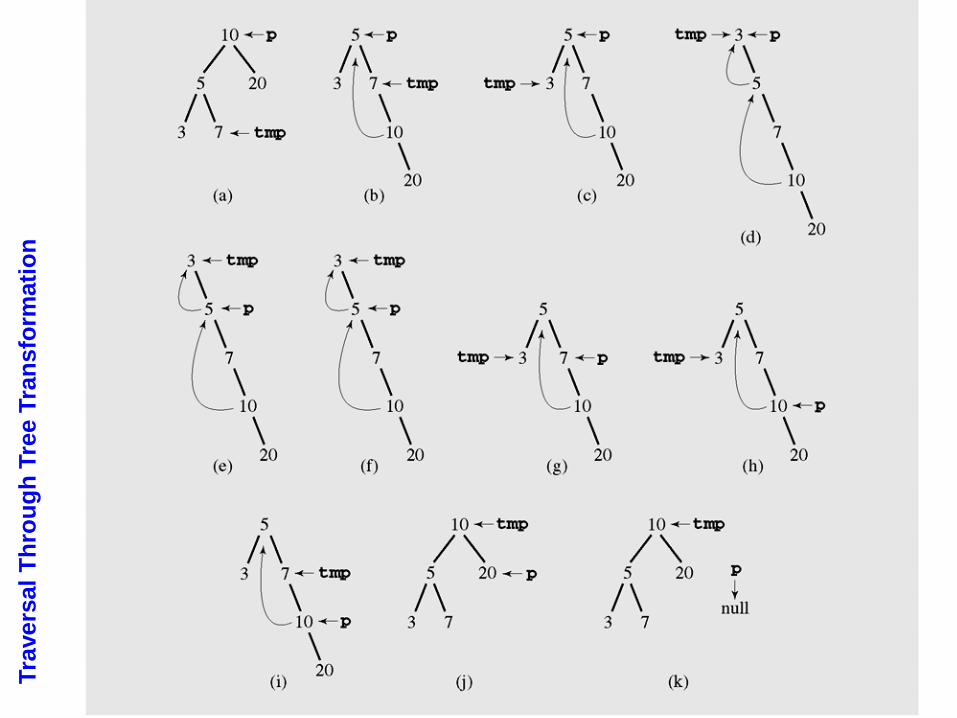
Traversal Through Tree Transformation

Figure 6-20 Implementation of the Morris algorithm for inorder traversal

47

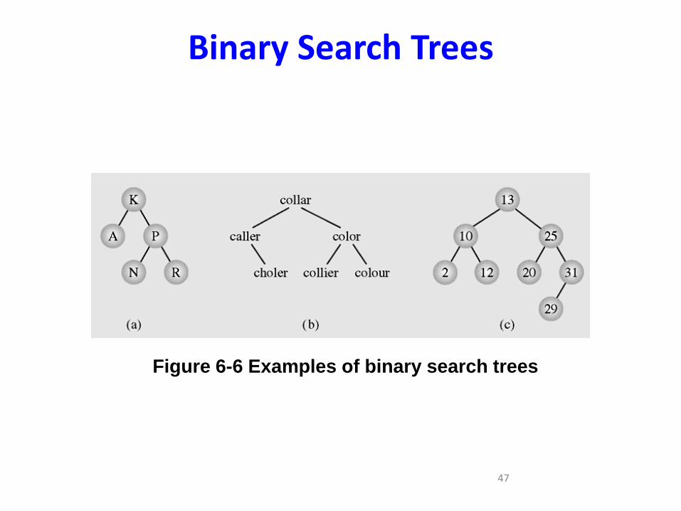
Binary Search Trees

Figure 6-6 Examples of binary search trees

48

Searching a Binary Search Tree (continued)

• The internal path length (IPL) is the sum of all path lengths of all nodes

• It is calculated by summing Σ(i – 1)li over all levels i, where li is the number of nodes on level I

• A depth of a node in the tree is determined by the path length

• An average depth, called an average pathlength, is given by the formula IPL/n, which depends on the shape of the tree

49

Insertion

Figure 6-22 Inserting nodes into binary search trees

50

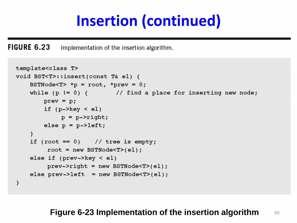
Insertion (continued)

Figure 6-23 Implementation of the insertion algorithm

51

Insertion (continued)

Figure 6-25 Inserting nodes into a threaded tree

52

Deletion in BSTs

• There are three cases of deleting a node from the binary search tree:

– The node is a leaf; it has no children

– The node has one child

– The node has two children

53

Deletion (continued)

Figure 6-26 Deleting a leaf

Figure 6-27 Deleting a node with one child

54

Deletion by Merging

• Making one tree out of the two subtrees of the node and then attaching it to the node’s parent is called deleting by merging

Figure 6-28 Summary of deleting by merging

55

Deletion by Copying

• If the node has two children, the problem can be reduced to:

– The node is a leaf

– The node has only one nonempty child

• Solution: replace the key being deleted with its immediate predecessor (or successor)

• A key’s predecessor is the key in the rightmost node in the left subtree

56

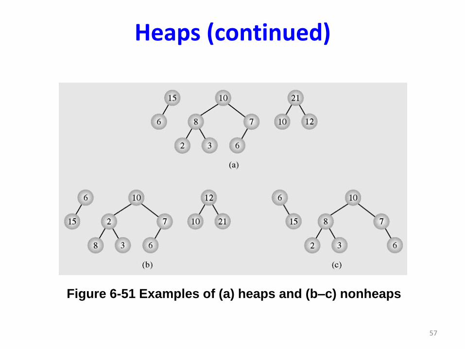
Heaps

• A particular kind of binary tree, called a heap, has two properties:

– The value of each node is greater than or equal to the values stored in each of its children

– The tree is perfectly balanced, and the leaves in the last level are all in the leftmost positions

• These two properties define a max heap

• If “greater” in the first property is replaced with “less,” then the definition specifies a min heap

57

Heaps (continued)

Figure 6-51 Examples of (a) heaps and (b–c) nonheaps

58

Heaps (continued)

Figure 6-52 The array [2 8 6 1 10 15 3 12 11] seen as a tree

59

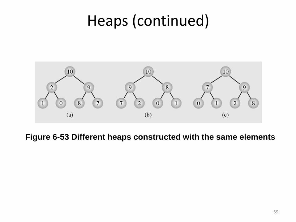
Heaps (continued)

Figure 6-53 Different heaps constructed with the same elements

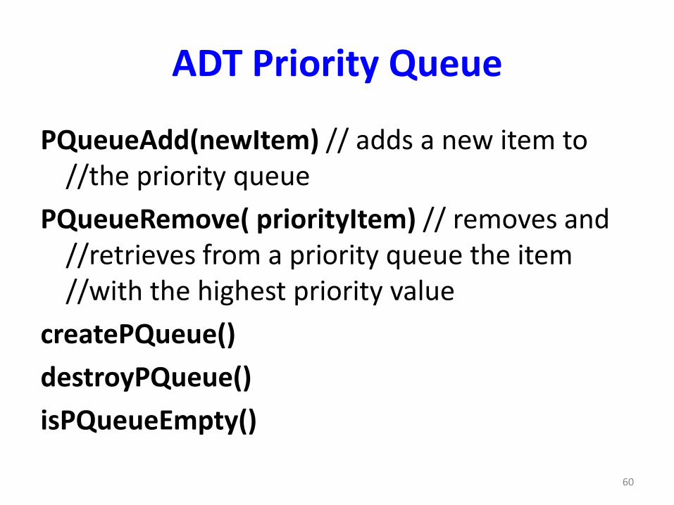
ADT Priority Queue

PQueueAdd(newItem) // adds a new item to //the priority queue

PQueueRemove( priorityItem) // removes and //retrieves from a priority queue the item //with the highest priority value

createPQueue()

destroyPQueue()

isPQueueEmpty()

60

Implementations of ADT Priority Queue

• With an array of pointers

61

62Operating Systems

. . .

0

1

n-1

i

.

.

.

.

.

.

front

rear

. . .

Queue

Pointer

. . .Priority headers

. . .

63

Heaps as Priority Queues

Figure 6-54 Enqueuing an element to a heap

64

Heaps as Priority Queues (continued)

Figure 6-55 Dequeuing an element from a heap

65

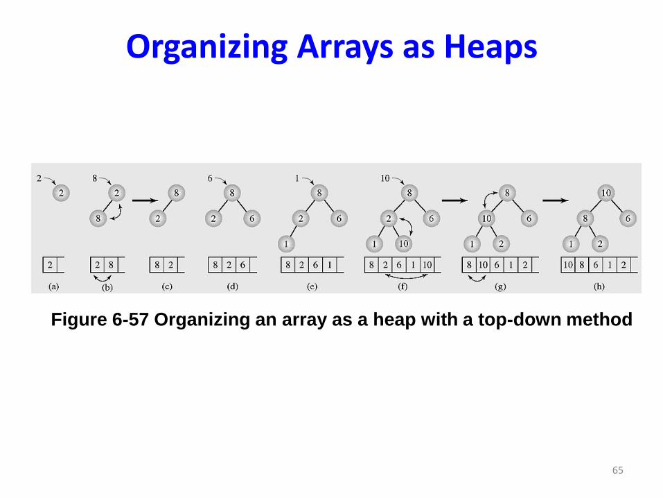
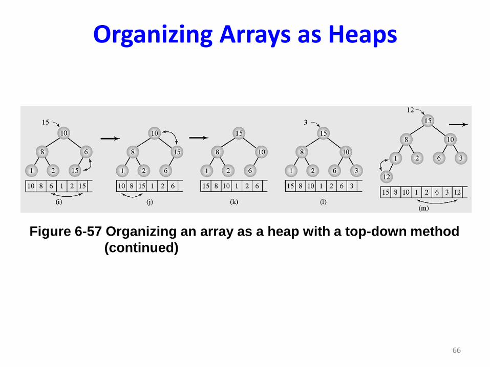
Organizing Arrays as Heaps

Figure 6-57 Organizing an array as a heap with a top-down method

66



(continued)

67



(continued)

68

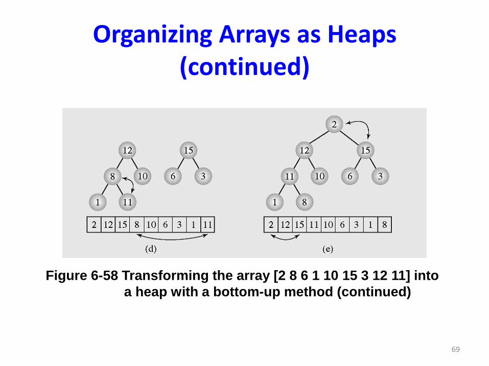
Organizing Arrays as Heaps (continued)

Figure 6-58 Transforming the array [2 8 6 1 10 15 3 12 11] into

a heap with a bottom-up method

69



a heap with a bottom-up method (continued)

70



a heap with a bottom-up method (continued)

71

Polish Notation and Expression Trees

• Polish notation is a special notation for propositional logic that eliminates all parentheses from formulas

• The compiler rejects everything that is not essential to retrieve the proper meaning of formulas rejecting it as “syntactic sugar”

72

Polish Notation and Expression Trees (continued)

Figure 6-59 Examples of three expression trees and results

of their traversals

7373

Balancing a Tree

• A binary tree is height-balanced or balanced if the difference in height of both subtrees of any node in the tree is either zero or one

• A tree is considered perfectly balanced if it is balanced and all leaves are to be found on one level or two levels

• Did not do this: next time

Data Structures -...

Documents

Transcript of Data Structures -...