1 Data Science - High dimensional regression

Data Science - High dimensionalregression

SummaryLinear models are popular methods for providing a regression of aresponse variable Y , that depends on covariates (X1, . . . ,Xp). Weintroduce the problem of high dimensional regression and providesome real examples where standard linear models methods are notwell suited. Then, we propose some statistical resolution through theLASSO estimator and the Boosting algorithm. A practical sessionis proposed in the end of this Lecture, since the knowledge of thesemodern methods is needed in many fields.

1 Back to linear models

1.1 Sum of squares minimization

In a standard linear model, we have at our disposal (Xi, Yi) supposed to belinked with

Yi =Xtiβ

∗+ εi,1 ≤ i ≤ n.

In particular, each observation Xi is described by p variables (X1i , . . . ,X

pi ),

so that the former relation should be understood as

Yi =p

∑j=1

β∗jXji + εi,1 ≤ i ≤ n.

We aim to recover the unknown β∗.

● A classical “optimal” estimator is the MLE :

βMLE ∶= arg maxβ∈Rp

L(β, (Xi, Yi)1≤i≤n),

whereL denotes the likelihood of the parameter β given the observations(Xi, Yi)1≤i≤n.

● Generically, (εi)1≤i≤n is assumed to be i.i.d. replications of a centeredand squared integrale noise

E[ε] = 0 E[ε2] <∞.

A standard assumption even relies on the Gaussian structure of the errorsεi ∼ N (0,1) and in this case, the log-likelihood leads to the minimiza-tion of the sum of square and

βMLE ∶= arg minβ∈Rp

n

∑i=1

∥Yi −Xtiβ∥

2

´¹¹¹¹¹¹¹¹¹¹¹¹¹¹¹¹¹¹¹¹¹¹¹¹¹¹¹¹¹¹¹¹¹¹¹¹¹¹¹¸¹¹¹¹¹¹¹¹¹¹¹¹¹¹¹¹¹¹¹¹¹¹¹¹¹¹¹¹¹¹¹¹¹¹¹¹¹¹¶∶=J(β)

. (1)

1.2 Matricial traduction & resolution

From a matricial point of view, the linear model can we written as follows :

Y =Xβ0 + ε, Y ∈ Rn,X ∈Mn,p(R), β0 ∈ Rp

In this lecture, we will consider situations where p varies (typically increases)with n.

It is an easy exercice to check that (1) leads to

βMLE ∶= (XtX)−1XtY .

2 Data Science - High dimensional regression

This can be obtained while remarking that J is a convex function, that pos-sesses a unique minimizer if and only if XtX has a full rank, meaning that Jis indeed strongly convex :

D2J =XtX,

which is a squared p × p symmetric and positive matrix. It is non degenerate ifXtX has full rank, meaning that necessarily p ≤ n.

PROPOSITION 1. — βMLE is an unbiased estimator of β0 such that

● If ε ∼ N (0, σ2) : ∥X(ˆbetaMLE−β∗)∥22

σ2 ∼ χ2p

●

E [∥X(βMLE − β

∗)∥22n

] =σ2p

n

Main requirement : XtX must be full rank (invertible) !

1.3 Difficulties in large dimensional case

Example One measures micro-array datasets built from a huge amount ofprofile genes expression. From a statistical point of view, we expect to findamong the p variables that describe X important ones.

Number of genes p (of order thousands). Number of samples n (of orderhundred).

-Yi expression level of one gene on sample i

-Xi = (Xi,1, . . . ,Xi,p) biological signal (DNA micro-arrays)

Diagnostic help : healthy or ill ?

● Select among the genes meaningful elements : discover a cognitive linkbetween DNA and the gene expression level.

● Find an algorithm with good prediction of the response ?

Linear model ? Difficult to imagine : p > n !

● XtX is an p × p matrix, but its rank is lower than n. If n << p, then

rk(XtX) ≤ n << p.

● Consequence : the Gram matrix XtX is not invertible and even veryill-conditionned (most of the eigenvalues are 0 !)

● The linear model βMLE completely fails.● One standard “improvement" : use the ridge regression with an additio-

nal penalty :

βRidgen = arg minβ∈Rp

∥Y −Xβ∥22 + λ∥β∥22

The ridge regression is a particular case of penalized regression. Thepenalization is still convex w.r.t. β and can be easily solved.

● We will attempt to describe a better suited penalized regression for highdimensional regression.

● Our goal : find a method that permits to find βn such that :— Select features among the p variables.— Can be easily computed with numerical softs.— Possess some statistical guarantees.

1.4 Goals

Important and nowadays questions :

● What is a good framework for high dimensional regression ? A goodmodel is required.

● How can we estimate ? An efficient algorithm is necessary.● How can we measure the performances : prediction of Y ? Feature se-

lection in β ? What are we looking for ?● Statistical guarantees ? Some mathematical theorems ?

3 Data Science - High dimensional regression

2 Penalized regression

2.1 Important balance : bias-variance tradeoff

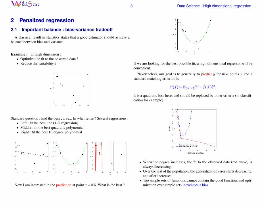
A classical result in statistics states that a good estimator should achieve abalance between bias and variance.

Example : In high dimension :● Optimize the fit to the observed data ?● Reduce the variability ?

Standard question : find the best curve... In what sense ? Several regressions :● Left : fit the best line (1-D regression)● Middle : fit the best quadratic polynomial● Right : fit the best 10-degree polynomial

Now I am interested in the prediction at point x = 0.5. What is the best ?

If we are looking for the best possible fit, a high dimensional regressor will beconvenient.

Nevertheless, our goal is to generally to predict y for new points x and astandard matching criterion is

C(f) ∶= E(X,Y )[Y − f(X)]2.

It is a quadratic loss here, and should be replaced by other criteria (in classifi-cation for example).

● When the degree increases, the fit to the observed data (red curve) isalways decreasing.

● Over the rest of the population, the generalization error starts decreasing,and after increases.

● Too simple sets of functions cannot contain the good function, and opti-mization over simple sets introduces a bias.

4 Data Science - High dimensional regression

● Too complex sets of functions may contain the good function but are toorich and generates high variance.

The former balance is illustrated by a very simple theorem.

Y = f(X) + ε with E[ε] = 0.

THÉORÈME 2. — For any estimator f , one has

C(f) = E[Y − f(X)]2

= E [Y −E[f(X)]]2

+E [E[f(X)] − f(X)]2

+E [Y − f(X)]2

● The blue term is a bias term.● The red term is a variance term.● The green term is the Bayes risk and is independent on the estimator f .

Statistical principle :

The empirical squared loss ∥Y − f(X)∥22,n mimics the bias. It is the sum ofsquares in (1). Important needs to introduce something to quantify the varianceof estimation : this is provided by a penalty term.

2.2 Ridge regression as a preliminary (insufficient)response

Ridge Ridge regression is like ordinary linear regression, but it shrinks theestimated coefficients towards zero. The ridge coefficients are defined by sol-ving

βRidge ∶= arg minβ∈Rp

∥Y −Xtβ∥22 + λ∥β∥22

Here λ ≥ 0 is a tuning parameter, which controls the strength of the penaltyterm. Write βRidge as the ridge solution. Note that :● When λ = 0, we get the linear regression estimate

● When λ = +∞, we get βRidge = 0● For λ in between, we are balancing two ideas : fitting a linear model ofY on X , and shrinking the coefficients.

Ridge with intercept When including an intercept term in the regression,we usually leave this coefficient unpenalized. Otherwise we could add someconstant amount c to the vector Y , and this would not result in the same solu-tion. Hence ridge regression with intercept solves

βRidge ∶= arg minc∈R,β∈Rp

∥Y − c −Xtβ∥22 + λ∥β∥22

If we center the columns of X , then the intercept estimate ends up just beingc = Y , so we usually just assume that Y and X have been centered and don’tinclude an intercept.

Also, the penalty term ∥β∥22 is unfair is the predictor variables are not on thesame scale. (Why ?) Therefore, if we know that the variables are not measuredin the same units, we typically scale the columns ofX (to have sample variance1), and then we perform ridge regression.

Bias and variance of the ridge regression The bias and variance are notquite as simple to write down for ridge regression as they were for linear re-gression (see Proposition 1) but closed-form expressions are still possible. Thegeneral trend is :● The bias increases as λ (amount of shrinkage) increases● The variance decreases as λ (amount of shrinkage) increases

Think : what is the bias at λ = 0 ? The variance at λ = +∞ ?

5 Data Science - High dimensional regression

● What you may (should) be thinking now : this only work for some valuesof λ so how would we choose λ in practice ? As you can imagine, oneway to do this involves cross-validation.

● What happens when we none of the true coefficients are small ? In otherwords, if all the true coefficients are moderate or large, is it still helpful toshrink the coeffi- cient estimates ? The answer is (perhaps surprisingly)still “yes”. But the advantage of ridge regression here is less dramatic,and the corresponding range for good values of λ is smaller.

Variable selection To the other extreme (of a subset of small coefficients),suppose that there is a group of true coefficients that are identically zero. Thatis, that the mean outcome doesn’t depend on these predictors at all, so they arecompletely extraneous.

The problem of picking out the relevant variables from a larger set is calledvariable selection. In the linear model setting, it means estimating some co-efficients to be exactly zero. Aside from predictive accuracy, this can be veryimportant for the purposes of model interpretation.

So how does ridge regression perform if a group of the true coefficients wasexactly zero ? The answer depends whether on we are interested in predictionor interpretation. In terms of prediction, the answer is effectively exactly thesame as what happens with a group of small true coefficients–there is no realdifference in the case of a large number of covariates with a null effect.

But for interpretation purposes, ridge regression does not provide as muchhelp as we would like. This is because it shrinks components of its estimate to-

ward zero, but never sets these components to be zero exactly (unless λ = +∞,in which case all components are zero). So strictly speaking, ridge regressiondoes not perform variable selection.

3 Sparsity : the Lasso re(s)volution

3.1 Sparsity assumption

An introductory example :● In many applications, p >> n but . . .● Important prior : many extracted feature in X are irrelevant● In an equivalent way : many coefficients in β0 are "exactly zero".● For example, if Y is the size of a tumor, it might be reasonable to suppose

that it can be expressed as a linear combination of genetic informationin the genome described in X . BUT most components of X will be zeroand most genes will be unimportant to predict Y :— We are looking for meaningful few genes— We are looking for the prediction of Y as well.

Dogmatic approach :● Sparsity : assumption that the unknown β0 we are looking for possesses

its major coordinates null. Only s of them are important :

s ∶= Card{1 ≤ i ≤ p∣β0(i) ≠ 0} .

● Sparsity assumption :s << n

● It permits to reduce the effective dimension of the problem.

6 Data Science - High dimensional regression

● Assume that the effective support of β0 is known, then

● If S is the support of β0, maybe XtSXS is full rank, and linear model

can be applied.Major issue : How could we find S ?

3.2 Lasso relaxation

Ideally, we would like to find β such that

βn = arg minβ∶∥β∥0≤s

∥Y −Xβ∥22,

meaning that the minimization is embbeded in a `0 ball.

In the previous lecture, we have seen that it is a constrained minimizationproblem of a convex function . . . A dual formulation is

arg minβ∶∥Y −Xβ∥2≤ε

{∥β∥0}

But : The `0 balls are not convex and not smooth !

● First (illusive) idea : explore all `0 subsets and minimize ! Bullshit since :

Csp subsets and p is large !

● Second idea (existing methods) : run some heuristic and greedy methodsto explore `0 balls and compute an approximation of βn. (See below)

● Good idea : use a convexification of the ∥∥0 norm (also referred to as aconvex relaxation method). How ?

Idea of the convex relaxation : instead of considering a variable z ∈ {0,1},imagine that z ∈ [0,1].

DÉFINITION 3. — [Convex Envelope] The convex envelope f∗ of a function fis the largest convex function below f .

THÉORÈME 4. — [Envelope of β z→ ∥β∥0]● On [−1,1]d, the convex envelope of β z→ ∥β∥0 is β z→ ∥β∥1.● On [−R,R]d, the convex envelope of β z→ ∥β∥0 is β z→ ∥β∥1

R.

Idea : Instead of solving the minimization problem :

∀s ∈ N min∥β∥0≤s

∥Y −Xβ∥22, (2)

we are looking for

∀C > 0 min∥.∥∗0(β)≤C

∥Y −Xβ∥22, (3)

What’s new ?● The function ∥.∥∗0 is convex and thus the above problem is a convex

minimization problem with convex constraints.● Since ∥.∥∗0(β) ≤ ∥β∥0, it is rather reasonnable to obtain sparse solutions.

In fact, solutions of (3) with a given C provide a lower bound of solu-tions of (2) with s ≤ C.

● If we are looking for good solutions of (2), then there must exists evenbetter solution to (3).

3.3 Geometrical interpretation (in 2 D)

Left : Level sets of ∥Y − Xβ∥22 and intersection with `1 ball. Right : Samewith `2 ball.

The left constraint problem is likely to obtain a sparse solution. Oppositely,the right constraint no !

In larger dimensions the balls are even more different :

7 Data Science - High dimensional regression

● Analytic point of view : why does the `1 norm induce sparsity ?● From the KKT conditions (see Lecture 1), it leads to a penalized crite-

rion

minβ∈Rp∶∥β∥1≤C

∥Y −Xβ∥22 ⇐⇒ minβ∈Rp

∥Y −Xβ∥22´¹¹¹¹¹¹¹¹¹¹¹¹¹¹¹¹¹¹¹¹¹¹¹¸¹¹¹¹¹¹¹¹¹¹¹¹¹¹¹¹¹¹¹¹¹¹¹¶Mimics the bias

+

Controls the variance­λ∥β∥1

● In the 1d case : arg minα∈R12∣x − α∣2 + λ∣x∣´¹¹¹¹¹¹¹¹¹¹¹¹¹¹¹¹¹¹¹¹¹¹¹¹¹¹¹¹¹¹¹¹¹¸¹¹¹¹¹¹¹¹¹¹¹¹¹¹¹¹¹¹¹¹¹¹¹¹¹¹¹¹¹¹¹¹¶

∶=ϕλ(x)

:

● The minimal value of ϕλ is reached at point x∗ when 0 ∈ ∂ϕλ(x∗). We

can check that x∗ is minimal iff— x∗ ≠ 0 and (x∗ − α) + λsgn(x∗) = 0.— x∗ = 0 and dϕ+λ(0) > 0 and dϕ−λ(0) < 0.PROPOSITION 5. — [Analytical minimization of ϕλ]

x∗ = sgn(α)[∣α∣ − λ]+ = arg minx∈R

{1

2∣x − α∣2 + λ∣x∣}

● For large values of λ, the minimum of ϕλ is reached at point 0.

3.4 Lasso estimator

We introduce the Least Absolute Shrinkage and Selection Operator :

∀λ > 0 βLasson = arg minβ∈Rp

∥Y −Xβ∥22 + λ∥β∥1

The above criterion is convex w.r.t. β.

● Efficient algorithms to solve the LASSO, even for very large p.● The minimizer may not be unique since the above criterion is not stron-

gly convex.● Predictions XβLasson are always unique.● λ is a penalty constant that must be carefully chosen.● A large value of λ leads to a very sparse solution, with an important bias.● A low value of λ yields overfitting with no penalization (too much im-

portant variance).● We will see that a careful balance between s, n and p exists. These para-

meters as well as the variance of the noise σ2 influence a “good " choiceof λ.

Alternative formulation :

βLasson = arg minβ∈Rp∶∥β∥1≤C

∥Y −Xβ∥22

3.5 Principle of the MM algorithm

Algorithm is needed to solve the minimization problem

arg minβ∈Rp

∥Y −Xβ∥22 + λ∥β∥1´¹¹¹¹¹¹¹¹¹¹¹¹¹¹¹¹¹¹¹¹¹¹¹¹¹¹¹¹¹¹¹¹¹¹¹¹¹¹¹¹¹¹¹¹¹¹¹¹¹¹¹¹¹¹¹¸¹¹¹¹¹¹¹¹¹¹¹¹¹¹¹¹¹¹¹¹¹¹¹¹¹¹¹¹¹¹¹¹¹¹¹¹¹¹¹¹¹¹¹¹¹¹¹¹¹¹¹¹¹¹¹¶

∶=ϕλ(β)

.

An efficient method follows the method of "Minimize Majorization" and isreferred to as MM method.● MM are useful for the minimization of a convex function/maximization

of a concave one.● Geometric illustration

8 Data Science - High dimensional regression

● Idea : Build a sequence (βk)k≥0 that converges to the minimum of ϕλ.● A particular case of such a method is encountered with the E.M. algo-

rithm useful for clustering and mixture models.● MM algorithms are powerful, especially they can convert non-

differentiable problems to smooth ones.

1. A function g(β,βk) is said to majorize f at point βk if

g(βk ∣βk) = f(βk) and g(β∣βk) ≥ f(β),∀β ∈ Rp.

2. Then, we defineβk+1 = arg min

β∈Rpg(β∣βk)

3. We wish to find each time a function g(., βk) whose minimization iseasy.

4. An example with a quadratic majorizer of a non-smooth function :

5. Important remark : The MM is a descent algorithm :

f(βk+1) = g(βk+1∣βk) + f(βk+1) − g(βk+1∣βk)

≤ g(βk ∣βk) = f(βk) (4)

3.6 MM algorithm for the LASSO

We can deduce for the LASSO the coordinate descent algorithm

1. Define a sequence (βk)k≥0 ⇐⇒ find a suitable majorization.

2. g ∶ β z→ ∥Y − Xβ∥2 is convex, whose Hessian matrix is XtX . ATaylor’s expansion leads to

∀y ∈ Rp g(y) ≤ g(x) + ⟨∇g(x), y − x⟩ + ρ(X)∥y − x∥2,

where ρ(X) is the spectral radius of X .

3. We are naturally driven to upper bound ϕλ as

ϕλ(β) ≤ ϕλ(βk) + ⟨∇g(βk), β − βk⟩ + ρ(X)∥β − βk∥22 + λ∥β∥1

= ψ(βk) + ρ(X) ∥β − (βk −∇g(βk)

ρ(X))∥

2

2

+ λ∥β∥1 ∶= ϕk(β)

The important point with this majorization is that it is “tensorized” : eachcoordinates acts separately on ϕk(β).

4. To minimize the majorization of ϕλ, we then use the above propositionof soft-thresholding :● Define

βjk ∶= βjk −∇g(βk)

j/ρ(X).

● Compute

βjk+1 = sgn(βjk)max [∣βjk ∣ −

2λ

ρ(X)]+

4 Running the Lasso

4.1 Choice of the regularization parameter

It is an important issue to obtain a good performance of the method, andcould be almost qualified as a “tarte à la crême” issue.

We won’t provide a sharp presentation of the best known results to keep thelevel understandable.

9 Data Science - High dimensional regression

It is important to have in mind the extremely favorable situation of an almostorthogonal design :

XtX

n≃ Ip.

In this case solving the lasso is equivalent to

minw

1

2n∥Xty −w∥

22 + λ∥w∥1

Solutions are given by ST (Soft-Thresholding) :

wj = STλ (1

nXtjy) = STλ (θ0j +

1

nXtjε)

We would like to keep the useless coefficients to 0, which requires that

λ ≥1

nXtjε,∀j ∈ J

c0 .

The random variables 1nXtjε are i.i.d. with a variance σ2/n.

PROPOSITION 6. — The expectation of the maximum of p − s Gaussian stan-dard variables is

E[ max1≤i≤p−s

Xi] ∼√

2 log(p − s).

We are naturally driven to the choice

λ = Aσ

√log p

n, with A >

√2.

Precisely :P (∀j ∈ Jc0 ∶ ∣X

tjε∣ ≤ nλ) ≥ 1 − p1−A

2/2.

4.2 Theoretical consistency

An additionnal remark is that we expect STλ z→ Id to obtain a consistencyresult. It means that λz→ 0, so that

log p

nz→ 0

Hence, a good behaviour of the lasso can be expected only if we have the nextdimensional settings :

pn = O(exp(n1−ξ)).

THÉORÈME 7. — Assume that log p << n, X has norm 1 and εi ∼ N (0, σ2),then under a coherence assumption on the design matrix XtX , one has

i) With high probability, J(θn) ⊂ J0.

ii) There exists C such that, with high probability,

∥X(θn − θ0)∥22

n≤C

κ2σ2s0 log p

n,

where κ2 is a positive constant that depends on the correlations inXtX .

One can also find results on the exact support recovery, as well as someweaker results without any coherence assumption.

N.B. : Such a coherence is measured through the almost orthogonality of thecolums of X . It can be traduced in terms of

∣ supi≠j

⟨Xi,Xj⟩∣ ≤ ε.

4.3 Practical calibration of λ

In practice, λ is generally chosen according to a criterion that is data de-pendent, e.g. a criterion that is calibrated on the observations through a cross-validation approach. In general, the packages implement this automatic choiceof the regularization parameter with a CV option.

10 Data Science - High dimensional regression

5 Numerical example

5.1 Very brief R code

5.1.1 About the use of the Ridge regression

library(lars)data(diabetes)library(MASS)diabetes.ridge <- lm.ridge(diabetes$y ~ diabetes$x,

lambda=seq(0,10,0.05))plot(diabetes.ridge, lwd=3)

0 2 4 6 8 10

−40

−20

020

x$lambda

t(x$

coef

)

We can see that the influence of the regularization parameter λ of the ridgeregression is important ! But a good choice of λ is difficult and should be data-driven. That is why a cross-validation procedure is needed. Does the ridgeregression performs variable selection ?

5.1.2 About the use of the Lasso regression

library(lars)data(diabetes)diabetes.lasso = lars(diabetes$x, diabetes$y,

type=’lasso’)plot(diabetes.lasso)

Lars algorithm : solves the Lasso less efficiently than the coordinate descentalgorithm.

* * * * * * * * * * * * *

0.0 0.2 0.4 0.6 0.8 1.0

−50

00

500

|beta|/max|beta|

Sta

ndar

dize

d C

oeffi

cien

ts

* * * * ** *

* * * * * *

**

**

* * * * * * * * *

* * **

* * * * * * * * *

* * * * * * **

* *

* *

*

* * * * * * * * * *

* *

*

* * * ** * * *

* ** *

** * * * * * * *

* * * * *

* *

**

* * ** * *

* **

* * * * * * * * * * * * *

LASSO

52

18

46

9

0 2 3 4 5 7 8 10 12

Typical output of the Lars software :● The greater `1 norm, the lower λ● Sparse solution with small values of the ∥.∥1 norm.

We can see that each variable of the diabetes dataset enter the model suc-cessively as long as λ decreases to 0. Again, the choice of λ should be donecarefully with a data-driven criterion.

5.2 Removing the bias of the Lasso

Signal processing example :

11 Data Science - High dimensional regression

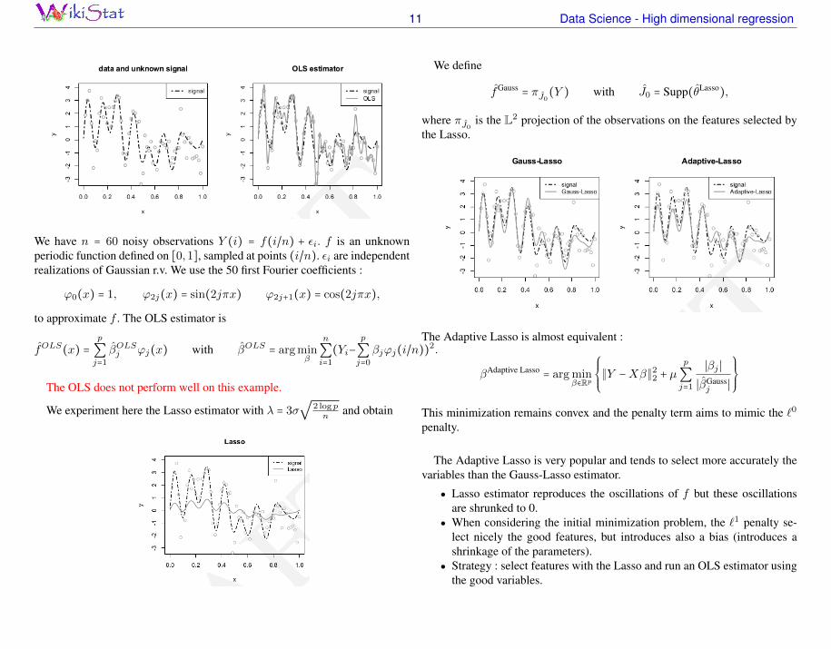
We have n = 60 noisy observations Y (i) = f(i/n) + εi. f is an unknownperiodic function defined on [0,1], sampled at points (i/n). εi are independentrealizations of Gaussian r.v. We use the 50 first Fourier coefficients :

ϕ0(x) = 1, ϕ2j(x) = sin(2jπx) ϕ2j+1(x) = cos(2jπx),

to approximate f . The OLS estimator is

fOLS(x) =p

∑j=1

βOLSj ϕj(x) with βOLS = arg minβ

n

∑i=1

(Yi−p

∑j=0

βjϕj(i/n))2.

The OLS does not perform well on this example.

We experiment here the Lasso estimator with λ = 3σ√

2 log pn

and obtain

We define

fGauss= πJ0(Y ) with J0 = Supp(θLasso

),

where πJ0 is the L2 projection of the observations on the features selected bythe Lasso.

The Adaptive Lasso is almost equivalent :

βAdaptive Lasso= arg min

β∈Rp

⎧⎪⎪⎨⎪⎪⎩

∥Y −Xβ∥22 + µp

∑j=1

∣βj ∣

∣βGaussj ∣

⎫⎪⎪⎬⎪⎪⎭

This minimization remains convex and the penalty term aims to mimic the `0

penalty.

The Adaptive Lasso is very popular and tends to select more accurately thevariables than the Gauss-Lasso estimator.

● Lasso estimator reproduces the oscillations of f but these oscillationsare shrunked to 0.

● When considering the initial minimization problem, the `1 penalty se-lect nicely the good features, but introduces also a bias (introduces ashrinkage of the parameters).

● Strategy : select features with the Lasso and run an OLS estimator usingthe good variables.

12 Data Science - High dimensional regression

6 HomeworkLength limitation : 6 pages !Deadline : 22th of February.Group of 2 students allowed.

1. You are asked first to follow the practical session on the Cookie database,that can be found in Moodle.You will need to install some packages with R.

2. Once you finish this practical session, please produce a short sum-mary with a few quantity of numerical illustrations and comments. Thiscontent could form the first part of your report. A special attention shouldbe paid to Ridge, Lasso regression and cross validation. Since this lastmethod has not been described in this lecture, I expect a brief descriptionof the method in the report and a discussion about its use.

3. To produce the same document, you are asked to complement your pro-duction with a gentle introduction to either

(a) Weak greedy algorithm (Boosting methods).● V. N. Temlyakov. Weak Greedy Algorithms. Advances in Com-

putational Mathe- matics, 12(2,3) :213-227, 2000.● J. A. Tropp. Greed is good : algorithmic results for sparse ap-

proximation. IEEE Trans. Inform. Theory, 50(10) :2231-2242,2004.

● M. Champion, C. Cierco-Ayrolles, S. Gadat, M. Vignes,Sparse regression and support recovery with L2-Boostingalgorithms. Journal of Statistical Planning and Inferencehttp ://dx.doi.org/10.1016/j.jspi.2014.07.006.

● P. Buhlmann and B. Yu. Boosting. Wiley Interdisciplinary Re-views : Computational Statistics 2, pages 69-74, 2010.

(b) Aggregation method (Exponential Weighting Aggregation)● A.Dalalyan, A. Tsybakov (2012). Sparse regression learning by

aggregation and Langevin Monte-Carlo. J. Comput. System Sci.,78(5), pp. 1423-1443.

● A. Dalalyan and A. Tsybakov (2009). Sparse Regression Lear-ning by Aggregation and Langevin Monte-Carlo. In COLT 2009

- The 22nd Conference on Learning Theory, Montreal, Quebec,Canada, June 18-21, 2009, pp. 1-10.

● J. Salmon and A. Dalalyan (2011). Optimal aggregation of affineestimators. In Journal of Machine Learning Research - Procee-dings Track 19, pp. 635-660.

The description of the algorithm could then form the second part of yourreport. You are asked to mainly describe the general behaviour of thealgorithm.

4. The last part of your report should compare this new algorithm with theLasso from a numerical point of view. You can either code the Boostingprocedure (in matlab, R, python, . . . ) or use a package. Please, provide areproducible simulation with sources code. This comparison should beunderstood from :● speed of the algorithm● statistical accuracy of the method● ability to handle large datasets● easy to use calibration of parameters