![[Flash] Modul Flash Sadana Production](https://static.fdocuments.in/doc/165x107/5571f80f49795991698c8ba3/flash-modul-flash-sadana-production.jpg)
Data Representation for Flash...
22
Data Representation for Flash Memories Anxiao (Andrew) Jiang Computer Science and Engineering Dept. Texas A&M University College Station, TX 77843, U.S.A. [email protected] Jehoshua Bruck Electrical Engineering Department California Institute of Technology Pasadena, CA 91125, U.S.A. [email protected] In this chapter, we introduce theories on data representation for flash memories. Flash mem- ories are a milestone in the development of the data storage technology. The applications of flash memories have expanded widely in recent years, and flash memories have become the dominating member in the family of non-volatile memories. Compared to magnetic record- ing and optical recording, flash memories are more suitable for many mobile-, embedded- and mass-storage applications. The reasons include their high speed, physical robustness, and easy integration with circuits. The representation of data plays a key role in storage systems. Like magnetic recording and optical recording, flash memories have their own distinct properties, including block erasure, iterative cell programming, etc. These distinct properties introduce very interesting coding problems that address many aspects of a successful storage system, which include efficient data modification, error correction, and more. In this chapter, we first introduce the flash memory model, then study some newly developed codes, including codes for rewriting data and the rank modulation scheme. A main theme is understanding how to store information in a medium that has asymmetric properties when it transits between different states. 1. Modelling Flash Memories The basic storage unit in a flash memory is a floating-gate transistor [3]. We also call it a cell. Charge (e.g., electrons) can be injected into the cell using the hot-electron injection mechanism or the Fowler-Nordheim tunnelling mechanism, and the injected charge is trapped in the cell. (Specifically, the charge is stored in the floating-gate layer of the transistor.) The charge can also be removed from the cell using the Fowler-Nordheim tunnelling mechanism. The amount of charge in a cell determines its threshold voltage, which can be measured. The operation of injecting charge into a cell is called writing (or programming), removing charge is called erasing, and measuring the charge level is called reading. If we use two discrete charge levels to store data, the cell is called single-level cell (SLC) and can store one bit. If we use q > 2 discrete charge levels to store data, the cell is called multi-level cell (MLC) and can store log 2 q bits. 4
-
Upload
duongkhanh -
Category
Documents
-
view
219 -
download
2
Transcript of Data Representation for Flash...

Data Representation for Flash Memories 53
Data Representation for Flash Memories
Anxiao (Andrew) Jiang and Jehoshua Bruck
0
Data Representation for Flash Memories
Anxiao (Andrew) JiangComputer Science and Engineering Dept.
Texas A&M UniversityCollege Station, TX 77843, U.S.A.
Jehoshua BruckElectrical Engineering Department
California Institute of TechnologyPasadena, CA 91125, U.S.A.
In this chapter, we introduce theories on data representation for flash memories. Flash mem-ories are a milestone in the development of the data storage technology. The applications offlash memories have expanded widely in recent years, and flash memories have become thedominating member in the family of non-volatile memories. Compared to magnetic record-ing and optical recording, flash memories are more suitable for many mobile-, embedded-and mass-storage applications. The reasons include their high speed, physical robustness,and easy integration with circuits.The representation of data plays a key role in storage systems. Like magnetic recording andoptical recording, flash memories have their own distinct properties, including block erasure,iterative cell programming, etc. These distinct properties introduce very interesting codingproblems that address many aspects of a successful storage system, which include efficientdata modification, error correction, and more. In this chapter, we first introduce the flashmemory model, then study some newly developed codes, including codes for rewriting dataand the rank modulation scheme. A main theme is understanding how to store informationin a medium that has asymmetric properties when it transits between different states.
1. Modelling Flash Memories
The basic storage unit in a flash memory is a floating-gate transistor [3]. We also call it a cell.Charge (e.g., electrons) can be injected into the cell using the hot-electron injection mechanismor the Fowler-Nordheim tunnelling mechanism, and the injected charge is trapped in the cell.(Specifically, the charge is stored in the floating-gate layer of the transistor.) The charge canalso be removed from the cell using the Fowler-Nordheim tunnelling mechanism. The amountof charge in a cell determines its threshold voltage, which can be measured. The operation ofinjecting charge into a cell is called writing (or programming), removing charge is called erasing,and measuring the charge level is called reading. If we use two discrete charge levels to storedata, the cell is called single-level cell (SLC) and can store one bit. If we use q > 2 discretecharge levels to store data, the cell is called multi-level cell (MLC) and can store log2 q bits.
4
Data Storage54
A prominent property of flash memories is block erasure. In a flash memory, cells are organizedinto blocks. A typical block contains about 105 cells. While it is relatively easy to inject chargeinto a cell, to remove charge from any cell, the whole block containing it must be erased to theground level (and then reprogrammed). This is called block erasure. The block erasure opera-tion not only significantly reduces speed, but also reduces the lifetime of the flash memory [3].This is because a block can only endure about 104 ∼ 106 erasures, after which the block maybreak down. Since the breaking down of a single block can make the whole memory stopworking, it is important to balance the erasures performed to different blocks. This is calledwear leveling. A commonly used wear-leveling technique is to balance erasures by movingdata among the blocks, especially when the data are revised [10].There are two main types of flash memories: NOR flash and NAND flash. A NOR flashmemory allows random access to its cells. A NAND flash partitions every block into multiplesections called pages, and a page is the unit of a read or write operation. Compared to NORflash, NAND flash may be much more restrictive on how its pages can be programmed, suchas allowing a page to be programmed only a few times before erasure [10]. However, NANDflash enjoys the advantage of higher cell density.The programming of cells is a noisy process. When charge is injected into a cell, the actualamount of injection is randomly distributed around the aimed value. An important thing toavoid during programming is overshooting, because to lower a cell’s level, erasure is needed.A commonly used approach to avoid overshooting is to program a cell using multiple roundsof charge injection. In each round, a conservative amount of charge is injected into the cell.Then the cell level is measured before the next round begins. With this approach, the chargelevel can gradually approach the target value and the programming precision is improved.The corresponding cost is the slowing down in the writing speed.After cells are programmed, the data are not necessarily error-proof, because the cell levelscan be changed by various errors over time. Some important error sources include write dis-turb and read disturb (disturbs caused by writing or reading), as well as leakage of charge fromthe cells (called the retention problem) [3]. The changes in the cell levels often have an asym-metric distribution in the up and the down directions, and the errors in different cells can becorrelated.In summary, flash memory is a storage medium with asymmetric properties. It is easy toincrease a cell’s charge level (which we shall call cell level), but very costly to decrease it due toblock erasure. The NAND flash may have more restrictions on reading and writing comparedto NOR flash. The cell programming uses multiple rounds of charge injection to shift thecell level monotonically up toward the target value, to avoid overshooting and improve theprecision. The cell levels can change over time due to various disturb mechanisms and theretention problem, and the errors can be asymmetric or correlated.
2. Codes for Rewriting Data
In this section, we discuss coding schemes for rewriting data in flash memories. The interestin this problem comes from the fact that if data are stored in the conventional way, even tochange one bit in the data, we may need to lower some cell’s level, which would lead to thecostly block erasure operation. It is interesting to see if there exist codes that allow data to berewritten many times without block erasure.The flash memory model we use in this section is the Write Asymmetric Memory (WAM)model [16].
Definition 1. WRITE ASYMMETRIC MEMORY (WAM) In a write asymmetric memory, there aren cells. Every cell has q ≥ 2 levels: levels 0, 1, · · · , q − 1. The level of a cell can only increase, notdecrease.
The Write Asymmetric Memory models the monotonic change of flash memory cells beforethe erasure operation. It is a special case of the generalized write-once memory (WOM) model,which allows the state transitions of cells to be any acyclic directed graph [6, 8, 29].Let us first look at an inspiring example. The code can write two bits twice in only threesingle-level cells. It was proposed by Rivest and Shamir in their celebrated paper that startedthe study of WOM codes [29].We always assume that before data are written into the cells, the cells are at level 0.
Example 2. We store two bits in three single-level cells (i.e., n = 3 and q = 2). The code is shown inFig. 1. In the figure, the three numbers in a circle represent the three cell levels, and the two numbersbeside the circle represent the two bits. The arrows represent the transition of the cells. As we can see,every cell level can only increase.The code allows us to write the two bits at least twice. For example, if want to write “10”, and laterrewrite them as “01”, we first elevate the cell levels to “0,1,0”, then elevate them to “0,1,1”.
Fig. 1. Code for writing two bits twice in three single-level cells.
In the above example, a rewrite can completely change the data. In practice, often multipledata variables are stored by an application, and every rewrite changes only one of them. Thejoint coding of these data variables are useful for increasing the number of rewrites supportedby coding. The rewriting codes in this setting have been named Floating Codes [16].
Definition 3. FLOATING CODEWe store k variables of alphabet size � in a write asymmetric memory (WAM) with n cells of q levels.Every rewrite changes one of the k variables.Let (c1, · · · , cn) ∈ {0, 1, · · · , q − 1}n denote the state of the memory (i.e., the levels of the n cells).Let (v1, · · · , vk) ∈ {0, 1, · · · , � − 1}k denote the data (i.e., the values of the k variables). For any

Data Representation for Flash Memories 55
A prominent property of flash memories is block erasure. In a flash memory, cells are organizedinto blocks. A typical block contains about 105 cells. While it is relatively easy to inject chargeinto a cell, to remove charge from any cell, the whole block containing it must be erased to theground level (and then reprogrammed). This is called block erasure. The block erasure opera-tion not only significantly reduces speed, but also reduces the lifetime of the flash memory [3].This is because a block can only endure about 104 ∼ 106 erasures, after which the block maybreak down. Since the breaking down of a single block can make the whole memory stopworking, it is important to balance the erasures performed to different blocks. This is calledwear leveling. A commonly used wear-leveling technique is to balance erasures by movingdata among the blocks, especially when the data are revised [10].There are two main types of flash memories: NOR flash and NAND flash. A NOR flashmemory allows random access to its cells. A NAND flash partitions every block into multiplesections called pages, and a page is the unit of a read or write operation. Compared to NORflash, NAND flash may be much more restrictive on how its pages can be programmed, suchas allowing a page to be programmed only a few times before erasure [10]. However, NANDflash enjoys the advantage of higher cell density.The programming of cells is a noisy process. When charge is injected into a cell, the actualamount of injection is randomly distributed around the aimed value. An important thing toavoid during programming is overshooting, because to lower a cell’s level, erasure is needed.A commonly used approach to avoid overshooting is to program a cell using multiple roundsof charge injection. In each round, a conservative amount of charge is injected into the cell.Then the cell level is measured before the next round begins. With this approach, the chargelevel can gradually approach the target value and the programming precision is improved.The corresponding cost is the slowing down in the writing speed.After cells are programmed, the data are not necessarily error-proof, because the cell levelscan be changed by various errors over time. Some important error sources include write dis-turb and read disturb (disturbs caused by writing or reading), as well as leakage of charge fromthe cells (called the retention problem) [3]. The changes in the cell levels often have an asym-metric distribution in the up and the down directions, and the errors in different cells can becorrelated.In summary, flash memory is a storage medium with asymmetric properties. It is easy toincrease a cell’s charge level (which we shall call cell level), but very costly to decrease it due toblock erasure. The NAND flash may have more restrictions on reading and writing comparedto NOR flash. The cell programming uses multiple rounds of charge injection to shift thecell level monotonically up toward the target value, to avoid overshooting and improve theprecision. The cell levels can change over time due to various disturb mechanisms and theretention problem, and the errors can be asymmetric or correlated.
2. Codes for Rewriting Data
In this section, we discuss coding schemes for rewriting data in flash memories. The interestin this problem comes from the fact that if data are stored in the conventional way, even tochange one bit in the data, we may need to lower some cell’s level, which would lead to thecostly block erasure operation. It is interesting to see if there exist codes that allow data to berewritten many times without block erasure.The flash memory model we use in this section is the Write Asymmetric Memory (WAM)model [16].
Definition 1. WRITE ASYMMETRIC MEMORY (WAM) In a write asymmetric memory, there aren cells. Every cell has q ≥ 2 levels: levels 0, 1, · · · , q − 1. The level of a cell can only increase, notdecrease.
The Write Asymmetric Memory models the monotonic change of flash memory cells beforethe erasure operation. It is a special case of the generalized write-once memory (WOM) model,which allows the state transitions of cells to be any acyclic directed graph [6, 8, 29].Let us first look at an inspiring example. The code can write two bits twice in only threesingle-level cells. It was proposed by Rivest and Shamir in their celebrated paper that startedthe study of WOM codes [29].We always assume that before data are written into the cells, the cells are at level 0.
Example 2. We store two bits in three single-level cells (i.e., n = 3 and q = 2). The code is shown inFig. 1. In the figure, the three numbers in a circle represent the three cell levels, and the two numbersbeside the circle represent the two bits. The arrows represent the transition of the cells. As we can see,every cell level can only increase.The code allows us to write the two bits at least twice. For example, if want to write “10”, and laterrewrite them as “01”, we first elevate the cell levels to “0,1,0”, then elevate them to “0,1,1”.
Fig. 1. Code for writing two bits twice in three single-level cells.
In the above example, a rewrite can completely change the data. In practice, often multipledata variables are stored by an application, and every rewrite changes only one of them. Thejoint coding of these data variables are useful for increasing the number of rewrites supportedby coding. The rewriting codes in this setting have been named Floating Codes [16].
Definition 3. FLOATING CODEWe store k variables of alphabet size � in a write asymmetric memory (WAM) with n cells of q levels.Every rewrite changes one of the k variables.Let (c1, · · · , cn) ∈ {0, 1, · · · , q − 1}n denote the state of the memory (i.e., the levels of the n cells).Let (v1, · · · , vk) ∈ {0, 1, · · · , � − 1}k denote the data (i.e., the values of the k variables). For any
Data Storage56
two memory states (c1, · · · , cn) and (c′1, · · · , c′n), we say (c1, · · · , cn) ≥ (c′1, · · · , c′n) if ci ≥ c′i fori = 1, · · · , n.A floating code has a decoding function Fd and an update function Fu. The decoding function
Fd : {0, 1, · · · , q − 1}n → {0, 1, · · · , �− 1}k
maps a memory state s ∈ {0, 1, · · · , q− 1}n to the stored data Fd(s) ∈ {0, 1, · · · , �− 1}k. The updatefunction (which represents a rewrite operation),
Fu : {0, 1, · · · , q − 1}n × {1, 2, · · · , k} × {0, 1, · · · , �− 1} → {0, 1, · · · , q − 1}n,
is defined as follows: if the current memory state is s and the rewrite changes the i-th variable to valuej ∈ {0, 1, · · · , �− 1}, then the rewrite operation will change the memory state to Fu(s, i, j) such thatFd(Fu(s, i, j)) is the data with the i-th variable changed to the value j. Naturally, since the memory isa write asymmetric memory, we require that Fu(s, i, j) ≥ s.Let t denote the number of rewrites (including the first write) guaranteed by the code. A floating codethat maximizes t is called optimal.
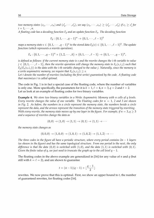
The code in Fig. 1 is in fact a special case of the floating code, where the number of variablesis only one. More specifically, the parameters for it is k = 1, � = 4, n = 3, q = 2 and t = 2.Let us look at an example of floating codes for two binary variables.
Example 4. We store two binary variables in a Write Asymmetric Memory with n cells of q levels.Every rewrite changes the value of one variable. The Floating codes for n = 1, 2 and 3 are shownin Fig. 2. As before, the numbers in a circle represent the memory state, the numbers beside a circlerepresent the data, and the arrows represent the transition of the memory state triggered by rewriting.With every rewrite, the memory state moves up by one layer in the figure. For example, if n = 3, q ≥ 3and a sequence of rewrites change the data as
(0, 0) → (1, 0) → (1, 1) → (0, 1) → (1, 1) → · · ·
the memory state changes as
(0, 0, 0) → (1, 0, 0) → (1, 0, 1) → (1, 0, 2) → (1, 1, 2) → · · ·
The three codes in the figure all have a periodic structure, where every period contains 2n − 1 layers(as shown in the figure) and has the same topological structure. From one period to the next, the onlydifference is that the data (0, 0) is switched with (1, 0), and the data (1, 1) is switched with (0, 1).Given the finite value of q, we just need to truncate the graph up to the cell level q − 1.
The floating codes in the above example are generalized in [16] for any value of n and q (butstill with k = � = 2), and are shown to guarantee
t = (n − 1)(q − 1) + � q − 12
�
rewrites. We now prove that this is optimal. First, we show an upper bound to t, the numberof guaranteed rewrites, for floating codes [16].
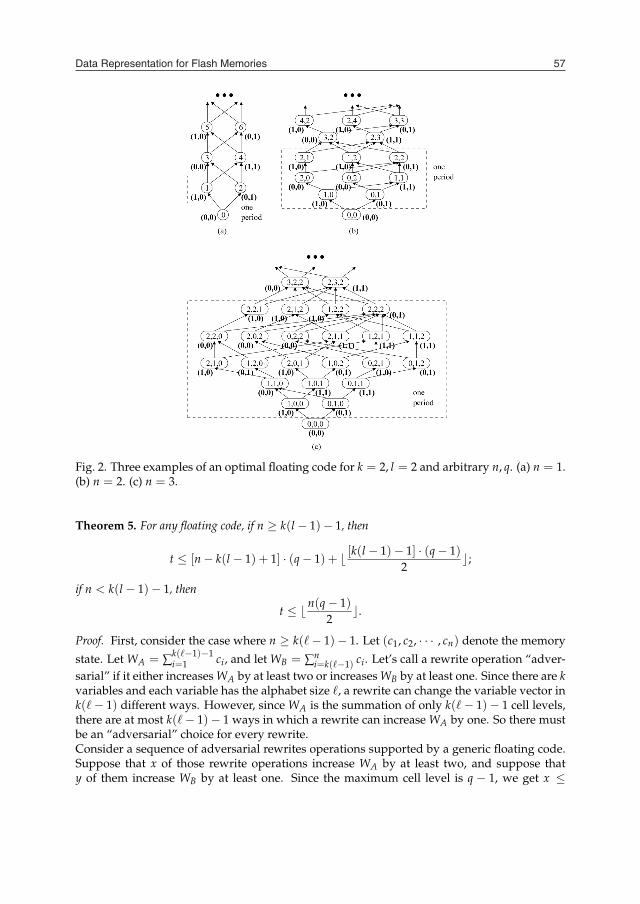
Fig. 2. Three examples of an optimal floating code for k = 2, l = 2 and arbitrary n, q. (a) n = 1.(b) n = 2. (c) n = 3.
Theorem 5. For any floating code, if n ≥ k(l − 1)− 1, then
t ≤ [n − k(l − 1) + 1] · (q − 1) + � [k(l − 1)− 1] · (q − 1)2
�;
if n < k(l − 1)− 1, then
t ≤ �n(q − 1)2
�.
Proof. First, consider the case where n ≥ k(�− 1)− 1. Let (c1, c2, · · · , cn) denote the memory
state. Let WA = ∑k(�−1)−1i=1 ci, and let WB = ∑n
i=k(�−1) ci. Let’s call a rewrite operation “adver-sarial” if it either increases WA by at least two or increases WB by at least one. Since there are kvariables and each variable has the alphabet size �, a rewrite can change the variable vector ink(�− 1) different ways. However, since WA is the summation of only k(�− 1)− 1 cell levels,there are at most k(�− 1)− 1 ways in which a rewrite can increase WA by one. So there mustbe an “adversarial” choice for every rewrite.Consider a sequence of adversarial rewrites operations supported by a generic floating code.Suppose that x of those rewrite operations increase WA by at least two, and suppose thaty of them increase WB by at least one. Since the maximum cell level is q − 1, we get x ≤
Data Representation for Flash Memories 57
two memory states (c1, · · · , cn) and (c′1, · · · , c′n), we say (c1, · · · , cn) ≥ (c′1, · · · , c′n) if ci ≥ c′i fori = 1, · · · , n.A floating code has a decoding function Fd and an update function Fu. The decoding function
Fd : {0, 1, · · · , q − 1}n → {0, 1, · · · , �− 1}k
maps a memory state s ∈ {0, 1, · · · , q− 1}n to the stored data Fd(s) ∈ {0, 1, · · · , �− 1}k. The updatefunction (which represents a rewrite operation),
Fu : {0, 1, · · · , q − 1}n × {1, 2, · · · , k} × {0, 1, · · · , �− 1} → {0, 1, · · · , q − 1}n,
is defined as follows: if the current memory state is s and the rewrite changes the i-th variable to valuej ∈ {0, 1, · · · , �− 1}, then the rewrite operation will change the memory state to Fu(s, i, j) such thatFd(Fu(s, i, j)) is the data with the i-th variable changed to the value j. Naturally, since the memory isa write asymmetric memory, we require that Fu(s, i, j) ≥ s.Let t denote the number of rewrites (including the first write) guaranteed by the code. A floating codethat maximizes t is called optimal.
The code in Fig. 1 is in fact a special case of the floating code, where the number of variablesis only one. More specifically, the parameters for it is k = 1, � = 4, n = 3, q = 2 and t = 2.Let us look at an example of floating codes for two binary variables.
Example 4. We store two binary variables in a Write Asymmetric Memory with n cells of q levels.Every rewrite changes the value of one variable. The Floating codes for n = 1, 2 and 3 are shownin Fig. 2. As before, the numbers in a circle represent the memory state, the numbers beside a circlerepresent the data, and the arrows represent the transition of the memory state triggered by rewriting.With every rewrite, the memory state moves up by one layer in the figure. For example, if n = 3, q ≥ 3and a sequence of rewrites change the data as
(0, 0) → (1, 0) → (1, 1) → (0, 1) → (1, 1) → · · ·
the memory state changes as
(0, 0, 0) → (1, 0, 0) → (1, 0, 1) → (1, 0, 2) → (1, 1, 2) → · · ·
The three codes in the figure all have a periodic structure, where every period contains 2n − 1 layers(as shown in the figure) and has the same topological structure. From one period to the next, the onlydifference is that the data (0, 0) is switched with (1, 0), and the data (1, 1) is switched with (0, 1).Given the finite value of q, we just need to truncate the graph up to the cell level q − 1.
The floating codes in the above example are generalized in [16] for any value of n and q (butstill with k = � = 2), and are shown to guarantee
t = (n − 1)(q − 1) + � q − 12
�
rewrites. We now prove that this is optimal. First, we show an upper bound to t, the numberof guaranteed rewrites, for floating codes [16].
Fig. 2. Three examples of an optimal floating code for k = 2, l = 2 and arbitrary n, q. (a) n = 1.(b) n = 2. (c) n = 3.
Theorem 5. For any floating code, if n ≥ k(l − 1)− 1, then
t ≤ [n − k(l − 1) + 1] · (q − 1) + � [k(l − 1)− 1] · (q − 1)2
�;
if n < k(l − 1)− 1, then
t ≤ �n(q − 1)2
�.
Proof. First, consider the case where n ≥ k(�− 1)− 1. Let (c1, c2, · · · , cn) denote the memory
state. Let WA = ∑k(�−1)−1i=1 ci, and let WB = ∑n
i=k(�−1) ci. Let’s call a rewrite operation “adver-sarial” if it either increases WA by at least two or increases WB by at least one. Since there are kvariables and each variable has the alphabet size �, a rewrite can change the variable vector ink(�− 1) different ways. However, since WA is the summation of only k(�− 1)− 1 cell levels,there are at most k(�− 1)− 1 ways in which a rewrite can increase WA by one. So there mustbe an “adversarial” choice for every rewrite.Consider a sequence of adversarial rewrites operations supported by a generic floating code.Suppose that x of those rewrite operations increase WA by at least two, and suppose thaty of them increase WB by at least one. Since the maximum cell level is q − 1, we get x ≤

Data Storage58
� [k(l−1)−1]·(q−1)2 � and y ≤ [n − k(l − 1) + 1] · (q − 1). So the number of rewrites supported by
a floating code is at most x + y ≤ [n − k(l − 1) + 1] · (q − 1) + � [k(l−1)−1]·(q−1)2 �.
The case where n < k(�− 1)− 1 can be analyzed similarly. Call a rewrite operation “adver-sarial” if it increases ∑n
i=1 ci by at least two. It can be shown that there is always a adversarial
choice for every rewrite, and any floating code can support at most t ≤ � n(q−1)2 � adversarial
rewrites.
When k = � = 2, the above theorem gives the bound t ≤ (n− 1)(q− 1)+ � q−12 �. It matches the
number of rewrites guaranteed by the floating codes of Example 4 (and their generalizationin [16]). So these codes are optimal.Let us pause a little to consider the two given examples. In Example 2, two bits can be writtentwice into the three single-level cells. The total number of bits written into the memory isfour (considering the whole history of rewriting), which is more than the number of bits thememory can store at any given time (which is three). In Example 4, every rewrite changes oneof two binary variables and therefore reflects one bit of information. Since the code guarantees(n − 1)(q − 1) + � q−1
2 � rewrites, the total amount of information “recorded” by the memory(again, over the history of rewriting) is (n − 1)(q − 1) + � q−1
2 � ≈ nq bits. In comparison, thenumber of bits the memory can store at any give time is only n log2 q.Why can the total amount of information written into the memory (over the multiple rewrites)exceed n log2 q, the maximum number of bits the memory can store at any give time? It is be-cause only the current value of the data needs to be remembered. Another way to understandit is that we are not using the cells sequentially. As an example, if there are n′ single level cellsand we increase one of their levels by one, there are n′ choices, which in fact reflects log2 n′
bits of information (instead of one bit).We now extend floating codes to a more general definition of rewriting codes. First, we usea directed graph to represent how rewrites may change the stored data. This definition wasproposed in [19].
Definition 6. GENERALIZED REWRITINGThe stored data is represented by a directed graph D = (VD , ED). The vertices VD represent all thevalues that the data can take. There is a directed edge (u, v) from u ∈ VD to v ∈ VD , v �= u, iff arewriting operation may change the stored data from value u to value v. The graph D is called the datagraph and the number of its vertices, corresponding to the input-alphabet size, is denoted by L = |VD|.Without loss of generality (w.l.o.g.), we assume the data graph to be strongly connected.
It is simple to see that when the above notion is applied to floating codes, the alphabet sizeL = �k, and the data graph D has constant in-degree and out-degree k(�− 1). The out-degreeof D reveals how much change in the data a rewrite operation can cause. It is an importantparameter. In the following, we show a rewriting code for this generalized rewriting model.The code, called Trajectory Code, was presented in [19].Let (c1, · · · , cn) ∈ {0, 1, q − 1}n denote the memory state. Let VD = {0, 1, · · · , L − 1} denotethe alphabet of the stored data. Let’s present the trajectory code step by step, starting with itsbasic building blocks.
Linear Code and Extended Linear Code
We first look at a Linear Code for the case n = L − 1 and q = 2. It was proposed by Rivest andShamir in [29].
Definition 7. LINEAR CODE FOR n = L − 1 AND q = 2The memory state (c1, · · · , cn) represents the data
n
∑i=1
ici mod (n + 1).
For every rewrite, change as few cells from level 0 to level 1 as possible to get the new data.
We give an example of the Linear Code.
Example 8. Let n = 7, q = 2 and L = 8. The data represented by the memory state (c1, · · · , c7) is
7
∑i=1
ici mod 8.
If the rewrites change the data as 0 → 3 → 5 → 2 → 4, the memory state can change as(0, 0, 0, 0, 0, 0, 0) → (0, 0, 1, 0, 0, 0, 0) → (0, 1, 1, 0, 0, 0, 0) → (0, 1, 1, 0, 1, 0, 0) → (0, 1, 1, 1, 1, 1, 0).
The following theorem shows that the number of rewrites enabled by the Linear Code isasymptotically optimal in n, the number of cells. It was proved in [29].
Theorem 9. The Linear Code guarantees at least n+14 + 1 rewrites.
Proof. We show that as long as at least n+12 cells are still of level 0, a rewrite will turn at most
two cells from level 0 to level 1. Let x ∈ {0, 1, · · · , n} denote the current data value, and lety ∈ {0, 1, · · · , n} denote the new data value to be written, where y �= x. Let z denote
y − x mod (n + 1).
If the cell cz is of level 0, we can simply change it to level 1. Otherwise, let
S = {i ∈ {1, · · · , n}|ci = 0},
and letT = {z − s mod (n + 1) | s ∈ S}.
Since |S| = |T| ≥ n+12 and |S ∪ T| < n (zero and z are in neither set), the set S ∩ T must be
nonempty. Their overlap indicates a solution to the equation
z = s1 + s2 mod (n + 1)
where s1 and s2 are elements of S.
When n ≥ L and q ≥ 2, we can generalize the Linear Code in the following way [19]. First,suppose n = L and q ≥ 2. We first use level 0 and level 1 to encode (as the Linear Codedoes), and let the memory state represent the data ∑n
i=1 ici mod n. (Note that rewrites herewill not change cn.) When the code can no longer support rewriting, we increase all celllevels (including cn) from 0 to 1, and start using cell levels 1 and 2 to store data in the sameway as above, except that now, the data represented by the memory state (c1, · · · , cn) usesthe formula ∑n
i=1 i(ci − 1) mod n. This process is repeated q − 1 times in total. The generaldecoding function is therefore
n
∑i=1
i(ci − cn) mod n.

Data Representation for Flash Memories 59
� [k(l−1)−1]·(q−1)2 � and y ≤ [n − k(l − 1) + 1] · (q − 1). So the number of rewrites supported by
a floating code is at most x + y ≤ [n − k(l − 1) + 1] · (q − 1) + � [k(l−1)−1]·(q−1)2 �.
The case where n < k(�− 1)− 1 can be analyzed similarly. Call a rewrite operation “adver-sarial” if it increases ∑n
i=1 ci by at least two. It can be shown that there is always a adversarial
choice for every rewrite, and any floating code can support at most t ≤ � n(q−1)2 � adversarial
rewrites.
When k = � = 2, the above theorem gives the bound t ≤ (n− 1)(q− 1)+ � q−12 �. It matches the
number of rewrites guaranteed by the floating codes of Example 4 (and their generalizationin [16]). So these codes are optimal.Let us pause a little to consider the two given examples. In Example 2, two bits can be writtentwice into the three single-level cells. The total number of bits written into the memory isfour (considering the whole history of rewriting), which is more than the number of bits thememory can store at any given time (which is three). In Example 4, every rewrite changes oneof two binary variables and therefore reflects one bit of information. Since the code guarantees(n − 1)(q − 1) + � q−1
2 � rewrites, the total amount of information “recorded” by the memory(again, over the history of rewriting) is (n − 1)(q − 1) + � q−1
2 � ≈ nq bits. In comparison, thenumber of bits the memory can store at any give time is only n log2 q.Why can the total amount of information written into the memory (over the multiple rewrites)exceed n log2 q, the maximum number of bits the memory can store at any give time? It is be-cause only the current value of the data needs to be remembered. Another way to understandit is that we are not using the cells sequentially. As an example, if there are n′ single level cellsand we increase one of their levels by one, there are n′ choices, which in fact reflects log2 n′
bits of information (instead of one bit).We now extend floating codes to a more general definition of rewriting codes. First, we usea directed graph to represent how rewrites may change the stored data. This definition wasproposed in [19].
Definition 6. GENERALIZED REWRITINGThe stored data is represented by a directed graph D = (VD , ED). The vertices VD represent all thevalues that the data can take. There is a directed edge (u, v) from u ∈ VD to v ∈ VD , v �= u, iff arewriting operation may change the stored data from value u to value v. The graph D is called the datagraph and the number of its vertices, corresponding to the input-alphabet size, is denoted by L = |VD|.Without loss of generality (w.l.o.g.), we assume the data graph to be strongly connected.
It is simple to see that when the above notion is applied to floating codes, the alphabet sizeL = �k, and the data graph D has constant in-degree and out-degree k(�− 1). The out-degreeof D reveals how much change in the data a rewrite operation can cause. It is an importantparameter. In the following, we show a rewriting code for this generalized rewriting model.The code, called Trajectory Code, was presented in [19].Let (c1, · · · , cn) ∈ {0, 1, q − 1}n denote the memory state. Let VD = {0, 1, · · · , L − 1} denotethe alphabet of the stored data. Let’s present the trajectory code step by step, starting with itsbasic building blocks.
Linear Code and Extended Linear Code
We first look at a Linear Code for the case n = L − 1 and q = 2. It was proposed by Rivest andShamir in [29].
Definition 7. LINEAR CODE FOR n = L − 1 AND q = 2The memory state (c1, · · · , cn) represents the data
n
∑i=1
ici mod (n + 1).
For every rewrite, change as few cells from level 0 to level 1 as possible to get the new data.
We give an example of the Linear Code.
Example 8. Let n = 7, q = 2 and L = 8. The data represented by the memory state (c1, · · · , c7) is
7
∑i=1
ici mod 8.
If the rewrites change the data as 0 → 3 → 5 → 2 → 4, the memory state can change as(0, 0, 0, 0, 0, 0, 0) → (0, 0, 1, 0, 0, 0, 0) → (0, 1, 1, 0, 0, 0, 0) → (0, 1, 1, 0, 1, 0, 0) → (0, 1, 1, 1, 1, 1, 0).
The following theorem shows that the number of rewrites enabled by the Linear Code isasymptotically optimal in n, the number of cells. It was proved in [29].
Theorem 9. The Linear Code guarantees at least n+14 + 1 rewrites.
Proof. We show that as long as at least n+12 cells are still of level 0, a rewrite will turn at most
two cells from level 0 to level 1. Let x ∈ {0, 1, · · · , n} denote the current data value, and lety ∈ {0, 1, · · · , n} denote the new data value to be written, where y �= x. Let z denote
y − x mod (n + 1).
If the cell cz is of level 0, we can simply change it to level 1. Otherwise, let
S = {i ∈ {1, · · · , n}|ci = 0},
and letT = {z − s mod (n + 1) | s ∈ S}.
Since |S| = |T| ≥ n+12 and |S ∪ T| < n (zero and z are in neither set), the set S ∩ T must be
nonempty. Their overlap indicates a solution to the equation
z = s1 + s2 mod (n + 1)
where s1 and s2 are elements of S.
When n ≥ L and q ≥ 2, we can generalize the Linear Code in the following way [19]. First,suppose n = L and q ≥ 2. We first use level 0 and level 1 to encode (as the Linear Codedoes), and let the memory state represent the data ∑n
i=1 ici mod n. (Note that rewrites herewill not change cn.) When the code can no longer support rewriting, we increase all celllevels (including cn) from 0 to 1, and start using cell levels 1 and 2 to store data in the sameway as above, except that now, the data represented by the memory state (c1, · · · , cn) usesthe formula ∑n
i=1 i(ci − 1) mod n. This process is repeated q − 1 times in total. The generaldecoding function is therefore
n
∑i=1
i(ci − cn) mod n.

Data Storage60
Now we extend the above code to n ≥ L cells. We divide the n cells into b = �n/L� groupsof size L (some cells may remain unused), and sequentially apply the above code to the firstgroup of L cells, then to the second group, and so on. We call this code the Extended LinearCode.
Theorem 10. Let 2 ≤ L ≤ n. The Extended Linear Code guarantees n(q − 1)/8 = Θ(nq) rewrites.
Proof. The Extended Linear Code essentially consists of (q − 1)� nL � ≥ (q−1)n
2L Linear Codes.
Code for Large Alphabet Size L
We now consider the case where L is larger than n. The rewriting code we present here willreduce it to the case n = L studied above [19]. We start by assuming that n < L ≤ 2
√n.
Construction 11. REWRITING CODE FOR n < L ≤ 2√
n
Let b be the smallest positive integer value that satisfies �n/b�b ≥ L.For i = 1, 2, . . . , b, let vi be a symbol from an alphabet of size �n/b� ≥ L1/b. We may represent anysymbol v ∈ {0, 1, · · · , L − 1} as a vector of symbols (v1, v2, . . . , vb). Partition the n flash cells into bgroups, each with �n/b� cells (some cells may remain unused). Encoding the symbol v into n cells isequivalent to the encoding of each vi into the corresponding group of �n/b� cells. As the alphabet sizeof each vi equals the number of cells it is to be encoded into, we can use the Extended Linear Code tostore vi.
Theorem 12. Let 16 ≤ n ≤ L ≤ 2√
n. The code in Construction 11 guarantees
n(q − 1) log n16 log L
= Θ(nq log n
log L)
rewrites.
Proof. We first show that for b – the smallest positive integer value that satisfies �n/b�b ≥ L –it holds that
b ≤ 2 log Llog n
.
Note that for all 1 ≤ x ≤√
n2 , we have �n/x�x ≥ nx/2. Since 16 ≤ n ≤ L ≤ 2�
√n�, it is easy to
verify that2 log Llog n
≤√
n2
.
Therefore,
�n log n2 log L
�2 log Llog n ≥ n
log Llog n = L,
which implies the upper bound for b.Using Construction 11, the number of rewrites possible is bounded by the number of rewritespossible for each of the b cell groups. By Theorem 10 and the above upper bound for b, this isat least
�nb� · q − 1
8≥ (
n log n2 log L
− 1)q − 1
8= Θ
(nq log n
log L
).
For the codes we have shown so far, we have not mentioned any constraint on the data graphD. Therefore, the above results hold for the case where the data graph is a complete graph.That is, a rewrite can change the data from any value to any other value. We now show that theabove codes are asymptotically optimal. For the Linear Code and the Extended Linear Code,this is easy to see, because every rewrite needs to increase some cell level, so the number ofrewrites cannot exceed n(q − 1) = O(nq). The following theorem shows that the rewritingcode in Construction 11 is asymptotically optimal, too [19].
Theorem 13. When n < L − 1 and the data graph D is a complete graph, a rewriting code canguarantee at most O(
nq log nlog L ) rewrites.
Proof. Let us consider some memory state s of the n flash cells, currently storing some valuev ∈ {0, 1, · · · , L − 1}. The next rewrite can change the data into any of the other L − 1 values.If we allow ourselves r operations of increasing a single cell level of the n flash cells (perhaps,operating on the same cell more than once), we may reach (n+r−1
r ) distinct new states. Let rbe the maximum integer sastisfying (n+r−1
r ) < L − 1. So for the next rewrite, we need at leastr + 1 such operations in the worst case. Since we have a total of n cells with q levels each, thenumber of rewrite operations is upper bounded by
n(q − 1)r + 1
≤ n(q − 1)
� log(L−1)1+log n �+ 1
= O(nq log n
log L).
Trajectory Code Construction
Let’s now consider more restricted rewrite operations. In many applications, a rewrite oftenchanges only a (small) part of the data. So let’s consider the case where a rewrite can changethe data to at most ∆ new values. This is the same as saying that in the data graph D, themaximum out-degree is ∆. We call such graph D a Bounded Out-degree Data Graph.The code to be shown is given the name Trajectory Code in [19]. Its idea is to record the pathin D along which the data changes, up to a certain length. When ∆ is small, this approach isparticularly helpful, because recording which outgoing edge a rewrite takes (one of ∆ choices)is more efficient than recording the new data value (one of L > ∆ choices).We first outline the construction of the Trajectory Code. Its parameters will be specified soon.Let n0, n1, n2, . . . , nd be d + 1 positive integers such that ∑d
i=0 ni = n is the number of cells. Wepartition the n cells into d + 1 groups, each with n0, n1, . . . , nd cells, respectively. We call themregisters S0, S1, . . . , Sd.The encoding uses the following basic scheme: we start by using register S0, called the anchor,to record the value of the initial data v0 ∈ {0, 1, · · · , L − 1}. For the next d rewrite operationswe use a differential scheme: denote by v1, . . . , vd ∈ {0, 1, · · · , L − 1} the next d values of therewritten data. In the i-th rewrite, 1 ≤ i ≤ d, we store in register Si the identity of the edge(vi−1, vi) ∈ ED . (ED and VD are the edge set and vertex set of the data graph D, respectively.)We do not require a unique label for all edges globally, but rather require that locally, for eachvertex in VD , its out-going edges have unique labels from {1, · · · , ∆}, where ∆ denotes themaximal out-degree in the data graph D.

Data Representation for Flash Memories 61
Now we extend the above code to n ≥ L cells. We divide the n cells into b = �n/L� groupsof size L (some cells may remain unused), and sequentially apply the above code to the firstgroup of L cells, then to the second group, and so on. We call this code the Extended LinearCode.
Theorem 10. Let 2 ≤ L ≤ n. The Extended Linear Code guarantees n(q − 1)/8 = Θ(nq) rewrites.
Proof. The Extended Linear Code essentially consists of (q − 1)� nL � ≥ (q−1)n
2L Linear Codes.
Code for Large Alphabet Size L
We now consider the case where L is larger than n. The rewriting code we present here willreduce it to the case n = L studied above [19]. We start by assuming that n < L ≤ 2
√n.
Construction 11. REWRITING CODE FOR n < L ≤ 2√
n
Let b be the smallest positive integer value that satisfies �n/b�b ≥ L.For i = 1, 2, . . . , b, let vi be a symbol from an alphabet of size �n/b� ≥ L1/b. We may represent anysymbol v ∈ {0, 1, · · · , L − 1} as a vector of symbols (v1, v2, . . . , vb). Partition the n flash cells into bgroups, each with �n/b� cells (some cells may remain unused). Encoding the symbol v into n cells isequivalent to the encoding of each vi into the corresponding group of �n/b� cells. As the alphabet sizeof each vi equals the number of cells it is to be encoded into, we can use the Extended Linear Code tostore vi.
Theorem 12. Let 16 ≤ n ≤ L ≤ 2√
n. The code in Construction 11 guarantees
n(q − 1) log n16 log L
= Θ(nq log n
log L)
rewrites.
Proof. We first show that for b – the smallest positive integer value that satisfies �n/b�b ≥ L –it holds that
b ≤ 2 log Llog n
.
Note that for all 1 ≤ x ≤√
n2 , we have �n/x�x ≥ nx/2. Since 16 ≤ n ≤ L ≤ 2�
√n�, it is easy to
verify that2 log Llog n
≤√
n2
.
Therefore,
�n log n2 log L
�2 log Llog n ≥ n
log Llog n = L,
which implies the upper bound for b.Using Construction 11, the number of rewrites possible is bounded by the number of rewritespossible for each of the b cell groups. By Theorem 10 and the above upper bound for b, this isat least
�nb� · q − 1
8≥ (
n log n2 log L
− 1)q − 1
8= Θ
(nq log n
log L
).
For the codes we have shown so far, we have not mentioned any constraint on the data graphD. Therefore, the above results hold for the case where the data graph is a complete graph.That is, a rewrite can change the data from any value to any other value. We now show that theabove codes are asymptotically optimal. For the Linear Code and the Extended Linear Code,this is easy to see, because every rewrite needs to increase some cell level, so the number ofrewrites cannot exceed n(q − 1) = O(nq). The following theorem shows that the rewritingcode in Construction 11 is asymptotically optimal, too [19].
Theorem 13. When n < L − 1 and the data graph D is a complete graph, a rewriting code canguarantee at most O(
nq log nlog L ) rewrites.
Proof. Let us consider some memory state s of the n flash cells, currently storing some valuev ∈ {0, 1, · · · , L − 1}. The next rewrite can change the data into any of the other L − 1 values.If we allow ourselves r operations of increasing a single cell level of the n flash cells (perhaps,operating on the same cell more than once), we may reach (n+r−1
r ) distinct new states. Let rbe the maximum integer sastisfying (n+r−1
r ) < L − 1. So for the next rewrite, we need at leastr + 1 such operations in the worst case. Since we have a total of n cells with q levels each, thenumber of rewrite operations is upper bounded by
n(q − 1)r + 1
≤ n(q − 1)
� log(L−1)1+log n �+ 1
= O(nq log n
log L).
Trajectory Code Construction
Let’s now consider more restricted rewrite operations. In many applications, a rewrite oftenchanges only a (small) part of the data. So let’s consider the case where a rewrite can changethe data to at most ∆ new values. This is the same as saying that in the data graph D, themaximum out-degree is ∆. We call such graph D a Bounded Out-degree Data Graph.The code to be shown is given the name Trajectory Code in [19]. Its idea is to record the pathin D along which the data changes, up to a certain length. When ∆ is small, this approach isparticularly helpful, because recording which outgoing edge a rewrite takes (one of ∆ choices)is more efficient than recording the new data value (one of L > ∆ choices).We first outline the construction of the Trajectory Code. Its parameters will be specified soon.Let n0, n1, n2, . . . , nd be d + 1 positive integers such that ∑d
i=0 ni = n is the number of cells. Wepartition the n cells into d + 1 groups, each with n0, n1, . . . , nd cells, respectively. We call themregisters S0, S1, . . . , Sd.The encoding uses the following basic scheme: we start by using register S0, called the anchor,to record the value of the initial data v0 ∈ {0, 1, · · · , L − 1}. For the next d rewrite operationswe use a differential scheme: denote by v1, . . . , vd ∈ {0, 1, · · · , L − 1} the next d values of therewritten data. In the i-th rewrite, 1 ≤ i ≤ d, we store in register Si the identity of the edge(vi−1, vi) ∈ ED . (ED and VD are the edge set and vertex set of the data graph D, respectively.)We do not require a unique label for all edges globally, but rather require that locally, for eachvertex in VD , its out-going edges have unique labels from {1, · · · , ∆}, where ∆ denotes themaximal out-degree in the data graph D.
Data Storage62
Intuitively, the first d rewrite operations are achieved by encoding the trajectory taken by theinput data sequence starting with the anchor data. After d such rewrites, we repeat the processby rewriting the next input from {0, 1, · · · , L − 1} in the anchor S0, and then continuing withd edge labels in S1, · · · , Sd.Let us assume a sequence of s rewrites have been stored thus far. To decode the last storedvalue all we need to know is s mod (d + 1). This is easily achieved by using �t/q� more cells(not specified in the previous d+ 1 registers), where t is the total number of rewrite operationswe would like to guarantee. For these �t/q� cells we employ a simple encoding scheme: inevery rewrite operation we arbitrarily choose one of those cells and raise its level by one.Thus, the total level in these cells equals s.The decoding process takes the value of the anchor S0 and then follows (s − 1) mod (d + 1)edges which are read consecutively from S1, S2, · · · . Notice that this scheme is appealing incases where the maximum out-degree of D is significantly lower than the alphabet size L.Note that each register Si, for i = 0, . . . , d, can be seen as a smaller rewriting code whose datagraph is a complete graph of either L vertices (for S0) or ∆ vertices (for S1, . . . , Sd). We use eitherthe Extended Linear Code or the code of Construction 11 for rewriting in the d + 1 registers.The parameters of the Trajectory Code are shown by the following construction. We assumethat n ≤ L ≤ 2
√n.
Construction 14. TRAJECTORY CODE FOR n ≤ L ≤ 2√
n
If ∆ ≤ � n log n2 log L �, let
d = �log L/ log n� = Θ(log L/ log n).
If � n log n2 log L � ≤ ∆ ≤ L, let
d = �log L/ log ∆� = Θ(log L/ log ∆).
In both cases, set the size of the d + 1 registers to n0 = �n/2� and ni = �n/(2d)� for i = 1, . . . d.If ∆ ≤ � n log n
2 log L �, apply the code of Construction 11 to register S0, and apply the Extended Linear Code
to registers S1, · · · , Sd. If � n log n2 log L � ≤ ∆ ≤ L, apply the code of Construction 11 to the d + 1 registers
S0, · · · , Sd.
The next three results show the asympotically optimality of the Trajectory Code (when ∆ issmall and large, respectively) [19].
Theorem 15. Let ∆ ≤ � n log n2 log L �. The Trajectory Code of Construction 14 guarantees Θ(nq) rewrites.
Proof. By Theorems 10 and 12, the number of rewrites possible in S0 is equal (up to constantfactors) to that of Si (i ≥ 1):
Θ(
n0q log n0log L
)= Θ
(nq log n
log L
)= Θ
(nqd
)= Θ (niq)
Thus the total number of rewrites guaranted by the Trajectory Code is d + 1 times the boundfor each register Si, which is Θ(nq).
Theorem 16. Let � n log n2 log L � ≤ ∆ ≤ L. The Trajectory Code of Construction 14 guarantees Θ
(nq log n
log ∆
)
rewrites.
Proof. By Theorem 12, the number of rewrites possible in S0 is:
Θ(
n0q log n0log L
)= Θ
(nq log n
log L
)
Similarly the number of rewrites possible in Si (i ≥ 1) is:
Θ(
niq log nilog ∆
)= Θ
(nq log nd log ∆
)= Θ
(nq log n
log L
).
Here we use the fact that as d ≤ log L it holds that d = o(n) and log ni = Θ(log n − log d) =Θ(log n). Notice that the two expressions above are equal. Thus, as in Theorem 15, we con-clude that the total number of rewrites guaranteed by the Trajectory Code is d + 1 times the
bound for each register Si, which is Θ(
nq log nlog ∆
).
The rewriting performance shown in the above theorem matches the bound shown in thefollowing theorem. We omit its proof, which interested readers can find in [19].
Theorem 17. Let ∆ > � n log n2 log L �. There exist data graphs D of maximum out-degree ∆ such that any
rewriting code for D can guarantee at most O(
nq log nlog ∆
)rewrites.
We have so far focused on rewriting codes with asymptotically optimal performance. It isinteresting to study rewriting codes that are strictly optimal, like the floating code in Exam-ple 4. Some codes of this kind have been studied in [16, 17]. In some practical applications,more specific forms of rewriting can be defined, and better rewriting codes can be found. Anexample is the Buffer Code defined for streaming data [2]. Besides studying the worst-case per-formance of rewriting codes, the expected rewriting performance is equally interesting. Somerewriting codes for expected performance are reported in [7, 19].
3. Rank Modulation
We focus our attention now on a new data representation scheme called Rank Modulation [21,23]. It uses the relative order of the cell levels, instead the absolute values of cell levels, torepresent data. Let us first understand the motivations for the scheme.Fast and accurate programming schemes for multi-level flash memories are a topic of signifi-cant research and design efforts. As mentioned before, the flash memory technology does notsupport charge removal from individual cells due to block erasure. As a result, an interativecell programming method is used. To program a cell, a sequence of charge injection opera-tions are used to shift the cell level cautiously and monotinically toward the target charge levelfrom below, in order to avoid undesired global erasures in case of overshoots. Consequently,the attempt to program a cell requires quite a few programming cycles, and it works only upto a moderate number of levels per cell.In addition to the need for accurate programming, the move to more levels in cells also ag-gravates the reliability problem. Compared to single-level cells, the higher storage capacity ofmulti-level cells are obtained at the cost of a smaller gap between adjacent cell levels. Many ofthe errors in flash memories are asymmetric, meaning that they shift the cell levels more likelyin one direction (up or down) than the other. Examples include the write disturbs, the readdisturbs, and the charge leakage. It will be interesting to design coding schemes that tolerateasymmetric errors better.

Data Representation for Flash Memories 63
Intuitively, the first d rewrite operations are achieved by encoding the trajectory taken by theinput data sequence starting with the anchor data. After d such rewrites, we repeat the processby rewriting the next input from {0, 1, · · · , L − 1} in the anchor S0, and then continuing withd edge labels in S1, · · · , Sd.Let us assume a sequence of s rewrites have been stored thus far. To decode the last storedvalue all we need to know is s mod (d + 1). This is easily achieved by using �t/q� more cells(not specified in the previous d+ 1 registers), where t is the total number of rewrite operationswe would like to guarantee. For these �t/q� cells we employ a simple encoding scheme: inevery rewrite operation we arbitrarily choose one of those cells and raise its level by one.Thus, the total level in these cells equals s.The decoding process takes the value of the anchor S0 and then follows (s − 1) mod (d + 1)edges which are read consecutively from S1, S2, · · · . Notice that this scheme is appealing incases where the maximum out-degree of D is significantly lower than the alphabet size L.Note that each register Si, for i = 0, . . . , d, can be seen as a smaller rewriting code whose datagraph is a complete graph of either L vertices (for S0) or ∆ vertices (for S1, . . . , Sd). We use eitherthe Extended Linear Code or the code of Construction 11 for rewriting in the d + 1 registers.The parameters of the Trajectory Code are shown by the following construction. We assumethat n ≤ L ≤ 2
√n.
Construction 14. TRAJECTORY CODE FOR n ≤ L ≤ 2√
n
If ∆ ≤ � n log n2 log L �, let
d = �log L/ log n� = Θ(log L/ log n).
If � n log n2 log L � ≤ ∆ ≤ L, let
d = �log L/ log ∆� = Θ(log L/ log ∆).
In both cases, set the size of the d + 1 registers to n0 = �n/2� and ni = �n/(2d)� for i = 1, . . . d.If ∆ ≤ � n log n
2 log L �, apply the code of Construction 11 to register S0, and apply the Extended Linear Code
to registers S1, · · · , Sd. If � n log n2 log L � ≤ ∆ ≤ L, apply the code of Construction 11 to the d + 1 registers
S0, · · · , Sd.
The next three results show the asympotically optimality of the Trajectory Code (when ∆ issmall and large, respectively) [19].
Theorem 15. Let ∆ ≤ � n log n2 log L �. The Trajectory Code of Construction 14 guarantees Θ(nq) rewrites.
Proof. By Theorems 10 and 12, the number of rewrites possible in S0 is equal (up to constantfactors) to that of Si (i ≥ 1):
Θ(
n0q log n0log L
)= Θ
(nq log n
log L
)= Θ
(nqd
)= Θ (niq)
Thus the total number of rewrites guaranted by the Trajectory Code is d + 1 times the boundfor each register Si, which is Θ(nq).
Theorem 16. Let � n log n2 log L � ≤ ∆ ≤ L. The Trajectory Code of Construction 14 guarantees Θ
(nq log n
log ∆
)
rewrites.
Proof. By Theorem 12, the number of rewrites possible in S0 is:
Θ(
n0q log n0log L
)= Θ
(nq log n
log L
)
Similarly the number of rewrites possible in Si (i ≥ 1) is:
Θ(
niq log nilog ∆
)= Θ
(nq log nd log ∆
)= Θ
(nq log n
log L
).
Here we use the fact that as d ≤ log L it holds that d = o(n) and log ni = Θ(log n − log d) =Θ(log n). Notice that the two expressions above are equal. Thus, as in Theorem 15, we con-clude that the total number of rewrites guaranteed by the Trajectory Code is d + 1 times the
bound for each register Si, which is Θ(
nq log nlog ∆
).
The rewriting performance shown in the above theorem matches the bound shown in thefollowing theorem. We omit its proof, which interested readers can find in [19].
Theorem 17. Let ∆ > � n log n2 log L �. There exist data graphs D of maximum out-degree ∆ such that any
rewriting code for D can guarantee at most O(
nq log nlog ∆
)rewrites.
We have so far focused on rewriting codes with asymptotically optimal performance. It isinteresting to study rewriting codes that are strictly optimal, like the floating code in Exam-ple 4. Some codes of this kind have been studied in [16, 17]. In some practical applications,more specific forms of rewriting can be defined, and better rewriting codes can be found. Anexample is the Buffer Code defined for streaming data [2]. Besides studying the worst-case per-formance of rewriting codes, the expected rewriting performance is equally interesting. Somerewriting codes for expected performance are reported in [7, 19].
3. Rank Modulation
We focus our attention now on a new data representation scheme called Rank Modulation [21,23]. It uses the relative order of the cell levels, instead the absolute values of cell levels, torepresent data. Let us first understand the motivations for the scheme.Fast and accurate programming schemes for multi-level flash memories are a topic of signifi-cant research and design efforts. As mentioned before, the flash memory technology does notsupport charge removal from individual cells due to block erasure. As a result, an interativecell programming method is used. To program a cell, a sequence of charge injection opera-tions are used to shift the cell level cautiously and monotinically toward the target charge levelfrom below, in order to avoid undesired global erasures in case of overshoots. Consequently,the attempt to program a cell requires quite a few programming cycles, and it works only upto a moderate number of levels per cell.In addition to the need for accurate programming, the move to more levels in cells also ag-gravates the reliability problem. Compared to single-level cells, the higher storage capacity ofmulti-level cells are obtained at the cost of a smaller gap between adjacent cell levels. Many ofthe errors in flash memories are asymmetric, meaning that they shift the cell levels more likelyin one direction (up or down) than the other. Examples include the write disturbs, the readdisturbs, and the charge leakage. It will be interesting to design coding schemes that tolerateasymmetric errors better.

Data Storage64
The Rank Modulation scheme is therefore proposed in [21, 23], whose aim is to eliminate boththe problem of overshooting while programming cells, and to tolerate asymmetric errors bet-ter. In this scheme, an ordered set of n cells stores the information in the permutation inducedby the charge levels of the cells. In this way, no discrete levels are needed (i.e., no need forthreshold levels) and only a basic charge-comparing operation (which is easy to implement) isrequired to read the permutation. If we further assume that the only programming operationallowed is raising the charge level of one of the cells above the current highest one (namely,push-to-top), then the overshoot problem is no longer relevant. Additionally, the technologymay allow in the future the decrease of all the charge levels in a block of cells by a constantamount smaller than the lowest charge level (block deflation), which would maintain their rela-tive values, and thus leave the information unchanged. This can eliminate a designated erasestep, by deflating the entire block whenever the memory is not in use.Let’s look at a simple example of rank modulation. Let [n] denote the set of integers{1, 2, · · · , n}.
Example 18. We partition the cells into groups of three cells each. Denote the three cells in a group bycell 1, cell 2, and cell 3. We use a permutation of [3] – [a1, a2, a3] – to represent the relative order of thethree cell levels as follows: cell a1 has the highest level, and cell a3 has the lowest level. (The cell levelsconsidered in this section are real numbers. So no two cells can practically have the same level.)The three cells in a group can introduce six possible permutations:[1, 2, 3], [1, 3, 2], [2, 1, 3], [2, 3, 1], [3, 1, 2], [3, 2, 1]. So they can store up to log2 6 bits of infor-mation. To write a permutation, we program the cells from the lowest level to the highest level. Forexample, if the permutation to write is [2, 3, 1], we first program cell 3 to make its level higher thanthat of cell 1, then program cell 2 to make its level higher than that of cell 3. This way, there is no riskof overshooting.
In this section, we use n to denote the number of cells in a group. As in the example, we usea permutation of [n] – [a1, a2, · · · , an] – to denote the relative order of the cell levels such thatcell a1 has the highest level and cell an has the lowest level.Once a new data representation method is defined, tools of coding are required to make ituseful. In this section, we focus on two tools: codes for rewriting, and codes for correctingerrors.
3.1 Rewriting Codes for Rank ModulationAssume that the only operation we allow for rewriting data is the “push-to-top” operation:injecting charge into a cell to make its level higher than all the other cell levels in the same cellgroup. Note that the push-to-top operation has no risk of overshooting. Then, how to designgood rewriting codes for rank modulation?Let � denote the alphabet size of the data symbol stored in a group of n cells. Let the alphabetof the data symbol be [�] = {1, 2, · · · , �}. Assume that a rewrite can change the data to anyvalue in [�]. In general, � might be smaller than n!, so we might end up having permutationsthat are not used. On the other hand, we can map several distinct permutations to the samesymbol i ∈ [�] in order to reduce the rewrite cost. We use Sn to denote the set of n! permuta-tions, and let Wn ⊆ Sn denote the set of states (i.e., the set of permutations) that are used torepresent information symbols. As before, for a rewriting code we can define two functions, adecoding function, Fd, and an update function, Fu.
Definition 19. The decoding function Fd : Wn → [�] maps every state s ∈ Wn to a value Fd(s)in [�]. Given an “old state” s ∈ Wn and a “new information symbol” i ∈ [�], the update functionFu : Wn × [�] → Wn produces a state Fu(s, i) such that Fd(Fu(s, i)) = i.
The more push-to-top operations are used for rewriting, the closer the highest cell level is tothe maximum level possible. Once it reaches the maximum level possible, block erasure willbe needed for the next rewrite. So we define the rewriting cost by measuring the number ofpush-to-top operations.
Definition 20. Given two states s1, s2 ∈ Wn, the cost of changing s1 into s2, denoted α(s1 → s2), isdefined as the minimum number of “push-to-the-top” operations needed to change s1 into s2.
For example, α([1, 2, 3] → [2, 1, 3]) = 1, α([1, 2, 3] → [3, 2, 1]) = 2.
Definition 21. The worst-case rewriting cost of a code is defined as maxs∈Wn ,i∈[�] α(s → Fu(s, i)).A code that minimized this cost is called optimal.
Before we present an optimal rewriting code, let’s first present a lower bound on the worst-case rewriting cost. Define the transition graph G = (V, E) as a directed graph with V = Sn,that is, with n! vertices representing the permutations in Sn. For any u, v ∈ V, there is adirected edge from u to v iff α(u → v) = 1. G is a regular digraph, because every vertex hasn − 1 incoming edges and n − 1 outgoing edges. The diameter of G is maxu,v∈V α(u → v) =n − 1.Given a vertex u ∈ V and an integer r ∈ {0, 1, . . . , n − 1}, define the ball centered at u withradius r as Bn
r (u) = {v ∈ V | α(u → v) ≤ r}, and define the sphere centered at u with radius ras Sn
r (u) = {v ∈ V | α(u → v) = r}. Clearly,
Bnr (u) =
⋃
0≤i≤rSn
r (u).
By a simple relabeling argument, both |Bnr (u)| and |Sn
r (u)| are independent of u, and so willbe denoted by |Bn
r | and |Snr | respectively.
Lemma 22. For any 0 ≤ r ≤ n − 1,
|Bnr | =
n!(n − r)!
|Snr | =
{1 r = 0
n!(n−r)! −
n!(n−r+1)! 1 ≤ r ≤ n − 1.
Proof. Fix a permutation u ∈ V. Let Pu be the set of permutations having the following prop-erty: for each permutation v ∈ Pu, the elements appearing in its last n − r positions appear inthe same relative order in u. For example, if n = 5, r = 2, u = [1, 2, 3, 4, 5] and v = [5, 2, 1, 3, 4],the last 3 elements of v – namely, 1, 3, 4 – have the same relative order in u. It is easy to seethat given u, when the elements occupying the first r positions in v ∈ Pu are chosen, the lastn − r positions become fixed. There are n(n − 1) · · · (n − r + 1) choices for occupying the firstr positions of v ∈ Pu, hence |Pu| = n!
(n−r)! . We will show that a vertex v is in Bnr (u) if and only
if v ∈ Pu.

Data Representation for Flash Memories 65
The Rank Modulation scheme is therefore proposed in [21, 23], whose aim is to eliminate boththe problem of overshooting while programming cells, and to tolerate asymmetric errors bet-ter. In this scheme, an ordered set of n cells stores the information in the permutation inducedby the charge levels of the cells. In this way, no discrete levels are needed (i.e., no need forthreshold levels) and only a basic charge-comparing operation (which is easy to implement) isrequired to read the permutation. If we further assume that the only programming operationallowed is raising the charge level of one of the cells above the current highest one (namely,push-to-top), then the overshoot problem is no longer relevant. Additionally, the technologymay allow in the future the decrease of all the charge levels in a block of cells by a constantamount smaller than the lowest charge level (block deflation), which would maintain their rela-tive values, and thus leave the information unchanged. This can eliminate a designated erasestep, by deflating the entire block whenever the memory is not in use.Let’s look at a simple example of rank modulation. Let [n] denote the set of integers{1, 2, · · · , n}.
Example 18. We partition the cells into groups of three cells each. Denote the three cells in a group bycell 1, cell 2, and cell 3. We use a permutation of [3] – [a1, a2, a3] – to represent the relative order of thethree cell levels as follows: cell a1 has the highest level, and cell a3 has the lowest level. (The cell levelsconsidered in this section are real numbers. So no two cells can practically have the same level.)The three cells in a group can introduce six possible permutations:[1, 2, 3], [1, 3, 2], [2, 1, 3], [2, 3, 1], [3, 1, 2], [3, 2, 1]. So they can store up to log2 6 bits of infor-mation. To write a permutation, we program the cells from the lowest level to the highest level. Forexample, if the permutation to write is [2, 3, 1], we first program cell 3 to make its level higher thanthat of cell 1, then program cell 2 to make its level higher than that of cell 3. This way, there is no riskof overshooting.
In this section, we use n to denote the number of cells in a group. As in the example, we usea permutation of [n] – [a1, a2, · · · , an] – to denote the relative order of the cell levels such thatcell a1 has the highest level and cell an has the lowest level.Once a new data representation method is defined, tools of coding are required to make ituseful. In this section, we focus on two tools: codes for rewriting, and codes for correctingerrors.
3.1 Rewriting Codes for Rank ModulationAssume that the only operation we allow for rewriting data is the “push-to-top” operation:injecting charge into a cell to make its level higher than all the other cell levels in the same cellgroup. Note that the push-to-top operation has no risk of overshooting. Then, how to designgood rewriting codes for rank modulation?Let � denote the alphabet size of the data symbol stored in a group of n cells. Let the alphabetof the data symbol be [�] = {1, 2, · · · , �}. Assume that a rewrite can change the data to anyvalue in [�]. In general, � might be smaller than n!, so we might end up having permutationsthat are not used. On the other hand, we can map several distinct permutations to the samesymbol i ∈ [�] in order to reduce the rewrite cost. We use Sn to denote the set of n! permuta-tions, and let Wn ⊆ Sn denote the set of states (i.e., the set of permutations) that are used torepresent information symbols. As before, for a rewriting code we can define two functions, adecoding function, Fd, and an update function, Fu.
Definition 19. The decoding function Fd : Wn → [�] maps every state s ∈ Wn to a value Fd(s)in [�]. Given an “old state” s ∈ Wn and a “new information symbol” i ∈ [�], the update functionFu : Wn × [�] → Wn produces a state Fu(s, i) such that Fd(Fu(s, i)) = i.
The more push-to-top operations are used for rewriting, the closer the highest cell level is tothe maximum level possible. Once it reaches the maximum level possible, block erasure willbe needed for the next rewrite. So we define the rewriting cost by measuring the number ofpush-to-top operations.
Definition 20. Given two states s1, s2 ∈ Wn, the cost of changing s1 into s2, denoted α(s1 → s2), isdefined as the minimum number of “push-to-the-top” operations needed to change s1 into s2.
For example, α([1, 2, 3] → [2, 1, 3]) = 1, α([1, 2, 3] → [3, 2, 1]) = 2.
Definition 21. The worst-case rewriting cost of a code is defined as maxs∈Wn ,i∈[�] α(s → Fu(s, i)).A code that minimized this cost is called optimal.
Before we present an optimal rewriting code, let’s first present a lower bound on the worst-case rewriting cost. Define the transition graph G = (V, E) as a directed graph with V = Sn,that is, with n! vertices representing the permutations in Sn. For any u, v ∈ V, there is adirected edge from u to v iff α(u → v) = 1. G is a regular digraph, because every vertex hasn − 1 incoming edges and n − 1 outgoing edges. The diameter of G is maxu,v∈V α(u → v) =n − 1.Given a vertex u ∈ V and an integer r ∈ {0, 1, . . . , n − 1}, define the ball centered at u withradius r as Bn
r (u) = {v ∈ V | α(u → v) ≤ r}, and define the sphere centered at u with radius ras Sn
r (u) = {v ∈ V | α(u → v) = r}. Clearly,
Bnr (u) =
⋃
0≤i≤rSn
r (u).
By a simple relabeling argument, both |Bnr (u)| and |Sn
r (u)| are independent of u, and so willbe denoted by |Bn
r | and |Snr | respectively.
Lemma 22. For any 0 ≤ r ≤ n − 1,
|Bnr | =
n!(n − r)!
|Snr | =
{1 r = 0
n!(n−r)! −
n!(n−r+1)! 1 ≤ r ≤ n − 1.
Proof. Fix a permutation u ∈ V. Let Pu be the set of permutations having the following prop-erty: for each permutation v ∈ Pu, the elements appearing in its last n − r positions appear inthe same relative order in u. For example, if n = 5, r = 2, u = [1, 2, 3, 4, 5] and v = [5, 2, 1, 3, 4],the last 3 elements of v – namely, 1, 3, 4 – have the same relative order in u. It is easy to seethat given u, when the elements occupying the first r positions in v ∈ Pu are chosen, the lastn − r positions become fixed. There are n(n − 1) · · · (n − r + 1) choices for occupying the firstr positions of v ∈ Pu, hence |Pu| = n!
(n−r)! . We will show that a vertex v is in Bnr (u) if and only
if v ∈ Pu.
Data Storage66
Suppose v ∈ Bnr (u). It follows that v can be obtained from u with at most r “push-to-the-top”
operations. Those elements pushed to the top appear in the first r positions of v, so the lastn − r positions of v contain elements which have the same relative order in u, thus, v ∈ Pu.Now suppose v ∈ Pu. For i ∈ [n], let vi denote the element in the i-th position of v. One cantransform u into v by sequentially pushing vr, vr−1, . . . , v1 to the top. Hence, v ∈ Bn
r (u).We conclude that |Bn
r (u)| = |P| = n!(n−r)! . Since Bn
r (u) =⋃
0≤i≤r Sni (u), the second claim
follows.
The following lemma shows a lower bound to the worst-case rewriting cost.
Lemma 23. Fix integers n and �, and define ρ(n, �) to be the smallest integer such that |Bnρ(n,�)| ≥ �.
For any code Wn and any state s ∈ Wn, there exists i ∈ [�] such that α(s → Fu(s, i)) ≥ ρ(n, �), i.e.,the worst-case rewriting cost of any code is at least ρ(n, �).
Proof. By the definition of ρ(n, �), |Bnρ(n,�)−1| < �. Hence, we can choose i ∈ [�] \ {Fd(s′) | s′ ∈
Bnρ(n,�)−1(s)}. Clearly, by our choice α(s → Fu(s, i)) ≥ ρ(n, �).
We now present a rewriting code construction. It will be shown that the code achieves theminimum worst-case rewriting cost. First, let us define the following notation.
Definition 24. A prefix sequence θ = [a(1), a(2), . . . , a(m)] is a sequence of m ≤ n distinct symbolsfrom [n]. The prefix set Pn(θ) ⊆ Sn is defined as all the permutations in Sn which start with thesequence θ.
We are now in a position to construct the code.
Construction 25. REWRITING CODE FOR RANK MODULATIONArbitrarily choose � distinct prefix sequences, θ1, . . . , θ�, each of length ρ(n, �). Let us define Wn =⋃
i∈[�] Pn(θi) and map the states of Pn(θi) to i, i.e., for each i ∈ [�] and s ∈ Pn(θi), set Fd(s) = i.Finally, to construct the update function Fu, given s ∈ Wn and some i ∈ [�], we do the following: let[a(1)i , a(2)i , . . . , a(ρ(n,�))
i ] be the first ρ(n, �) elements which appear in all the permutations in Pn(θi).
Apply push-to-top operations on the elements a(ρ(n,�))i , . . . , a(2)i , a(1)i in s to get a permutation s′ ∈
Pn(θi) for which, clearly, Fd(s′) = i. Set Fu(s, i) = s′.
Theorem 26. The code in Construction 25 is optimal in terms of minimizing the worst-case rewritingcost.
Proof. It is obvious from the description of Fu that the worst-case rewriting cost of the con-struction is at most ρ(n, �). By Lemma 23 this is also the best we can hope for.
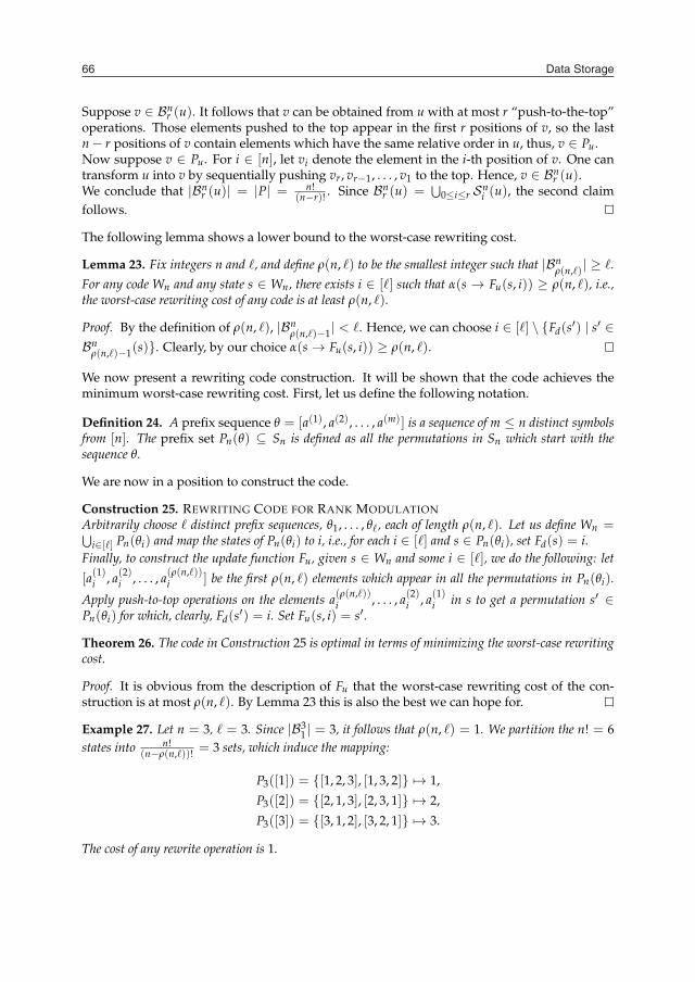
Example 27. Let n = 3, � = 3. Since |B31 | = 3, it follows that ρ(n, �) = 1. We partition the n! = 6
states into n!(n−ρ(n,�))! = 3 sets, which induce the mapping:
P3([1]) = {[1, 2, 3], [1, 3, 2]} �→ 1,
P3([2]) = {[2, 1, 3], [2, 3, 1]} �→ 2,
P3([3]) = {[3, 1, 2], [3, 2, 1]} �→ 3.
The cost of any rewrite operation is 1.
If a probability distribution is known for the rewritten data, we can also define the perfor-mance of codes based on the average rewriting cost. This is studied in [21], where an variable-length prefix-free code is optimized. It is shown that the average rewriting cost of this prefix-free code is within a small constant approximation ratio of the minimum possible cost of allcodes (prefix-free codes or not) under very mild conditions.
3.2 Error-correcting Codes for Rank ModulationError-correcting codes are often essential for the reliability of data. An error-correcting rankmodulation code is a subset of permutations that are far from each other based on some dis-tance measure. The distance between permutations needs to be defined appropriately accord-ing to the error model. In this section, we define distance as the number of adjacent transpo-sitions. We emphasize, however, that this is not the only way to define distance. The resultswe present here were shown in [23].Given a permutation, an adjacent transposition is the local exchange of two adja-cent elements in the permutation: [a1, . . . , ai−1, ai, ai+1, ai+2, . . . , an] is changed to[a1, . . . , ai−1, ai+1, ai, ai+2, . . . , an].In the rank modulation model, the minimal change to a permutation caused by charge-leveldrift is a single adjacent transposition. Let us measure the number of errors by the minimumnumber of adjacent transpositions needed to change the permutation from its original valueto its erroneous value. For example, if the errors change the permutation from [2, 1, 3, 4] to[2, 3, 4, 1], the number of errors is two, because at least two adjacent transpositions are neededto change one into the other: [2, 1, 3, 4] → [2, 3, 1, 4] → [2, 3, 4, 1].For two permutations A and B, define their distance, d(A, B), as the minimal number of adja-cent transpositions needed to change A into B. This distance measure is called the Kendall TauDistance in the statistics and machine-learning community [24], and it induces a metric overSn. If d(A, B) = 1, A and B are called adjacent. Any two permutations of Sn are at distance atmost n(n−1)
2 from each other. Two permutations of maximum distance are a reverse of eachother.
Basic Properties
Theorem 28. Let A = [a1, a2, . . . , an] and B = [b1, b2, . . . , bn] be two permutations of lengthn. Suppose that bp = an for some 1 ≤ p ≤ n. Let A′ = [a1, a2, . . . , an−1] and B′ =[b1, . . . , bp−1, bp+1, . . . , bn]. Then,
d(A, B) = d(A′, B′) + n − p.
The above theorem can be proved by induction. It shows a recursive algorithm for computingthe distance between two permutations. Let A = [a1, a2, . . . , an] and B = [b1, b2, . . . , bn] be twopermutations. For 1 ≤ i ≤ n, let Ai denote [a1, a2, . . . , ai], let Bi denote the subsequence of Bthat contains only those numbers in Ai, and let pi denote the position of ai in Bi. Then, sinced(A1, B1) = 0 and d(Ai, Bi) = d(Ai−1, Bi−1) + i − pi, for i = 2, 3, . . . , n, we get
d(A, B) = d(An, Bn) =(n − 1)(n + 2)
2−
n
∑i=2
pi.

Data Representation for Flash Memories 67
Suppose v ∈ Bnr (u). It follows that v can be obtained from u with at most r “push-to-the-top”
operations. Those elements pushed to the top appear in the first r positions of v, so the lastn − r positions of v contain elements which have the same relative order in u, thus, v ∈ Pu.Now suppose v ∈ Pu. For i ∈ [n], let vi denote the element in the i-th position of v. One cantransform u into v by sequentially pushing vr, vr−1, . . . , v1 to the top. Hence, v ∈ Bn
r (u).We conclude that |Bn
r (u)| = |P| = n!(n−r)! . Since Bn
r (u) =⋃
0≤i≤r Sni (u), the second claim
follows.
The following lemma shows a lower bound to the worst-case rewriting cost.
Lemma 23. Fix integers n and �, and define ρ(n, �) to be the smallest integer such that |Bnρ(n,�)| ≥ �.
For any code Wn and any state s ∈ Wn, there exists i ∈ [�] such that α(s → Fu(s, i)) ≥ ρ(n, �), i.e.,the worst-case rewriting cost of any code is at least ρ(n, �).
Proof. By the definition of ρ(n, �), |Bnρ(n,�)−1| < �. Hence, we can choose i ∈ [�] \ {Fd(s′) | s′ ∈
Bnρ(n,�)−1(s)}. Clearly, by our choice α(s → Fu(s, i)) ≥ ρ(n, �).
We now present a rewriting code construction. It will be shown that the code achieves theminimum worst-case rewriting cost. First, let us define the following notation.
Definition 24. A prefix sequence θ = [a(1), a(2), . . . , a(m)] is a sequence of m ≤ n distinct symbolsfrom [n]. The prefix set Pn(θ) ⊆ Sn is defined as all the permutations in Sn which start with thesequence θ.
We are now in a position to construct the code.
Construction 25. REWRITING CODE FOR RANK MODULATIONArbitrarily choose � distinct prefix sequences, θ1, . . . , θ�, each of length ρ(n, �). Let us define Wn =⋃
i∈[�] Pn(θi) and map the states of Pn(θi) to i, i.e., for each i ∈ [�] and s ∈ Pn(θi), set Fd(s) = i.Finally, to construct the update function Fu, given s ∈ Wn and some i ∈ [�], we do the following: let[a(1)i , a(2)i , . . . , a(ρ(n,�))
i ] be the first ρ(n, �) elements which appear in all the permutations in Pn(θi).
Apply push-to-top operations on the elements a(ρ(n,�))i , . . . , a(2)i , a(1)i in s to get a permutation s′ ∈
Pn(θi) for which, clearly, Fd(s′) = i. Set Fu(s, i) = s′.
Theorem 26. The code in Construction 25 is optimal in terms of minimizing the worst-case rewritingcost.
Proof. It is obvious from the description of Fu that the worst-case rewriting cost of the con-struction is at most ρ(n, �). By Lemma 23 this is also the best we can hope for.
Example 27. Let n = 3, � = 3. Since |B31 | = 3, it follows that ρ(n, �) = 1. We partition the n! = 6
states into n!(n−ρ(n,�))! = 3 sets, which induce the mapping:
P3([1]) = {[1, 2, 3], [1, 3, 2]} �→ 1,
P3([2]) = {[2, 1, 3], [2, 3, 1]} �→ 2,
P3([3]) = {[3, 1, 2], [3, 2, 1]} �→ 3.
The cost of any rewrite operation is 1.
If a probability distribution is known for the rewritten data, we can also define the perfor-mance of codes based on the average rewriting cost. This is studied in [21], where an variable-length prefix-free code is optimized. It is shown that the average rewriting cost of this prefix-free code is within a small constant approximation ratio of the minimum possible cost of allcodes (prefix-free codes or not) under very mild conditions.
3.2 Error-correcting Codes for Rank ModulationError-correcting codes are often essential for the reliability of data. An error-correcting rankmodulation code is a subset of permutations that are far from each other based on some dis-tance measure. The distance between permutations needs to be defined appropriately accord-ing to the error model. In this section, we define distance as the number of adjacent transpo-sitions. We emphasize, however, that this is not the only way to define distance. The resultswe present here were shown in [23].Given a permutation, an adjacent transposition is the local exchange of two adja-cent elements in the permutation: [a1, . . . , ai−1, ai, ai+1, ai+2, . . . , an] is changed to[a1, . . . , ai−1, ai+1, ai, ai+2, . . . , an].In the rank modulation model, the minimal change to a permutation caused by charge-leveldrift is a single adjacent transposition. Let us measure the number of errors by the minimumnumber of adjacent transpositions needed to change the permutation from its original valueto its erroneous value. For example, if the errors change the permutation from [2, 1, 3, 4] to[2, 3, 4, 1], the number of errors is two, because at least two adjacent transpositions are neededto change one into the other: [2, 1, 3, 4] → [2, 3, 1, 4] → [2, 3, 4, 1].For two permutations A and B, define their distance, d(A, B), as the minimal number of adja-cent transpositions needed to change A into B. This distance measure is called the Kendall TauDistance in the statistics and machine-learning community [24], and it induces a metric overSn. If d(A, B) = 1, A and B are called adjacent. Any two permutations of Sn are at distance atmost n(n−1)
2 from each other. Two permutations of maximum distance are a reverse of eachother.
Basic Properties
Theorem 28. Let A = [a1, a2, . . . , an] and B = [b1, b2, . . . , bn] be two permutations of lengthn. Suppose that bp = an for some 1 ≤ p ≤ n. Let A′ = [a1, a2, . . . , an−1] and B′ =[b1, . . . , bp−1, bp+1, . . . , bn]. Then,
d(A, B) = d(A′, B′) + n − p.
The above theorem can be proved by induction. It shows a recursive algorithm for computingthe distance between two permutations. Let A = [a1, a2, . . . , an] and B = [b1, b2, . . . , bn] be twopermutations. For 1 ≤ i ≤ n, let Ai denote [a1, a2, . . . , ai], let Bi denote the subsequence of Bthat contains only those numbers in Ai, and let pi denote the position of ai in Bi. Then, sinced(A1, B1) = 0 and d(Ai, Bi) = d(Ai−1, Bi−1) + i − pi, for i = 2, 3, . . . , n, we get
d(A, B) = d(An, Bn) =(n − 1)(n + 2)
2−
n
∑i=2
pi.

Data Storage68
Example 29. Let A = [1, 2, 3, 4] and B = [4, 2, 3, 1]. Then A1 = [1], A2 = [1, 2], A3 = [1, 2, 3],A4 = [1, 2, 3, 4], B1 = [1], B2 = [2, 1], B3 = [2, 3, 1], B4 = [4, 2, 3, 1]. We get
d(A1, B1) = 0,
d(A2, B2) = d(A1, B1) + 2 − p2 = 0 + 2 − 1 = 1,
d(A3, B3) = d(A2, B2) + 3 − p3 = 1 + 3 − 2 = 2,
d(A4, B4) = d(A3, B3) + 4 − p4 = 2 + 4 − 1 = 5.
Indeed, d(A, B) = (n−1)(n+2)2 − ∑n
i=2 pi =(4−1)(4+2)
2 − (1 + 2 + 1) = 5.
We now define a coordinate system for permutations. We fix A = [1, 2, . . . , n]. For everypermutation B = [b1, b2, . . . , bn], we define its coordinates as XB = (2 − p2, 3 − p3, . . . , n − pn).Here pi is defined as above for 2 ≤ i ≤ n. Clearly, if XB = (x1, x2, . . . , xn−1), then 0 ≤ xi ≤ ifor 1 ≤ i ≤ n − 1.
Example 30. Let A = [1, 2, 3, 4, 5]. Then XA = (0, 0, 0, 0). If B = [3, 4, 2, 1, 5], then XB =(1, 2, 2, 0). If B = [5, 4, 3, 2, 1], then XB = (1, 2, 3, 4). The full set of coordinates for n = 3 and n = 4are shown in Fig. 3 (a) and (c), respectively. �
The coordinate system is equivalent to a form of Lehmer code (or Lucas-Lehmer code, inver-sion table) [26]. It is easy to see that two permutations are identical if and only if they have thesame coordinates, and any vector (y1, y2, . . . , yn−1), 0 ≤ yi ≤ i for 1 ≤ i ≤ n − 1, is the coor-dinates of some permutation in Sn. So there is a one-to-one mapping between the coordinatesand the permutations.Let A ∈ Sn be a permutation. For any 0 ≤ r ≤ n(n−1)
2 , the set Br(A) = {B ∈ Sn | d(A, B) ≤ r}is a ball of radius r centered at A. A simple relabeling argument suffices to show that thesize of a ball does not depend on the choice of center. We use |Br| to denote |Br(A)| for anyA ∈ Sn. We are interested in finding the value of |Br|. The following theorem presents a wayto compute the size of a ball using polynomial multiplication.
Theorem 31. For 0 ≤ r ≤ n(n−1)2 , let er denote the coefficient of xr in the polynomial ∏n−1
i=1xi+1−1
x−1 .Then |Br| = ∑r
i=0 er.
Proof. Let A = [1, 2, . . . , n]. Let B = [b1, b2, . . . , bn] be a generic permutation. Let XB =(y1, y2, . . . , yn−1) be the coordinates of B. By the definition of coordinates, we get d(A, B) =
∑n−1i=1 yi. The number of permutations at distance r from A equals the number of integer
solutions to ∑n−1i=1 yi = r such that 0 ≤ yi ≤ i. That is equal to the coefficient of xr in the
polynomial ∏n−1i=1 (xi + xi−1 + · · ·+ 1) = ∏n−1
i=1xi+1−1
x−1 . Thus, there are exactly er permutationsat distance r from A, and |Br| = ∑r
i=0 ei.
Theorem 31 induces an upper bound for the sizes of error-correcting rank-modulation codes.By the sphere-packing principle, for such a code that can correct r errors, its size cannot exceedn!/|Br|.
Embedding of Permutation Adjacency Graph
Define the adjacency graph of permutations, G = (V, E), as follows. The graph G has |V| = n!vertices, which represent the n! permutations. Two vertices u, v ∈ V are adjacent if and only ifd(u, v) = 1. G is a regular undirected graph with degree n − 1 and diameter n(n−1)
2 . To studythe topology of G, we begin with the follow theorem.
Lemma 32. For two permutations A = [a1, a2, . . . , an] and B = [b1, b2, . . . , bn], let their coordinatesbe XA = (x1, x2, . . . , xn−1) and XB = (y1, y2, . . . , yn−1). If A and B are adjacent, then ∑n−1
i=1 |xi −yi| = 1.
The above lemma can be proved by induction. Interested readers can see [23] for details.Let Ln = (VL, EL) denote a 2 × 3 × · · · × n linear array graph. Ln has n! vertices VL. Eachvertex is assigned integer coordinates (x1, x2, . . . , xn−1), where 0 ≤ xi ≤ i for 1 ≤ i ≤ n − 1.The distance between vertices of Ln is the L1 distance, and two vertices are adjacent (i.e., havean edge between them) if and only if their distance is one.We now build a bijective map P : V → VL. Here V is the vertex set of the adjacency graphof permutations G = (V, E). For any u ∈ V and v ∈ VL, P(u) = v if and only if u, v havethe same coordinates. By Lemma 32, if two permutations are adjacent, their coordinates areadjacent in Ln. So we get:
Theorem 33. The adjacency graph of permutations is a subgraph of the 2 × 3 × · · · × n linear array.
We show some examples of the embedding in Fig. 3. It can be seen that while each permu-tation has n − 1 adjacent permutations, a vertex in the array can have a varied degree fromn − 1 to 2n − 3. Some edges of the array do not exist in the adjacency graph of permutations.
Fig. 3. Coordinates of permutations, and embedding the adjacency graph of permutations, G,in the 2 × 3 × · · · × n array, Ln. In the two arrays, the solid lines are the edges in both G andLn, and the dotted lines are the edges only in Ln. (a) Coordinates of permutations for n = 3.(b) Embedding G in Ln for n = 3. (c) Coordinates of permutations for n = 4. (d) EmbeddingG in Ln for n = 4.
The observation that the permutations’ adjacency graph is a subgraph of a linear array showsan approach to design error-correcting rank-modulation codes based on Lee-metric codes. Weskip the proof of the following theorem due to its simplicity.
Theorem 34. Let C be a Lee-metric error-correcting code of length n − 1, alphabet size no less than n,and minimum distance d. Let C′ be the subset of codewords of C that are contained in the array Ln.Then C′ is an error-correcting rank-modulation code with minimum distance at least d.
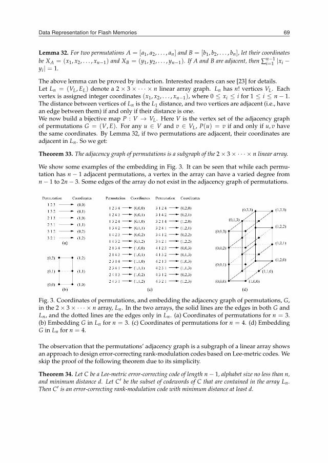
Data Representation for Flash Memories 69
Example 29. Let A = [1, 2, 3, 4] and B = [4, 2, 3, 1]. Then A1 = [1], A2 = [1, 2], A3 = [1, 2, 3],A4 = [1, 2, 3, 4], B1 = [1], B2 = [2, 1], B3 = [2, 3, 1], B4 = [4, 2, 3, 1]. We get
d(A1, B1) = 0,
d(A2, B2) = d(A1, B1) + 2 − p2 = 0 + 2 − 1 = 1,
d(A3, B3) = d(A2, B2) + 3 − p3 = 1 + 3 − 2 = 2,
d(A4, B4) = d(A3, B3) + 4 − p4 = 2 + 4 − 1 = 5.
Indeed, d(A, B) = (n−1)(n+2)2 − ∑n
i=2 pi =(4−1)(4+2)
2 − (1 + 2 + 1) = 5.
We now define a coordinate system for permutations. We fix A = [1, 2, . . . , n]. For everypermutation B = [b1, b2, . . . , bn], we define its coordinates as XB = (2 − p2, 3 − p3, . . . , n − pn).Here pi is defined as above for 2 ≤ i ≤ n. Clearly, if XB = (x1, x2, . . . , xn−1), then 0 ≤ xi ≤ ifor 1 ≤ i ≤ n − 1.
Example 30. Let A = [1, 2, 3, 4, 5]. Then XA = (0, 0, 0, 0). If B = [3, 4, 2, 1, 5], then XB =(1, 2, 2, 0). If B = [5, 4, 3, 2, 1], then XB = (1, 2, 3, 4). The full set of coordinates for n = 3 and n = 4are shown in Fig. 3 (a) and (c), respectively. �
The coordinate system is equivalent to a form of Lehmer code (or Lucas-Lehmer code, inver-sion table) [26]. It is easy to see that two permutations are identical if and only if they have thesame coordinates, and any vector (y1, y2, . . . , yn−1), 0 ≤ yi ≤ i for 1 ≤ i ≤ n − 1, is the coor-dinates of some permutation in Sn. So there is a one-to-one mapping between the coordinatesand the permutations.Let A ∈ Sn be a permutation. For any 0 ≤ r ≤ n(n−1)
2 , the set Br(A) = {B ∈ Sn | d(A, B) ≤ r}is a ball of radius r centered at A. A simple relabeling argument suffices to show that thesize of a ball does not depend on the choice of center. We use |Br| to denote |Br(A)| for anyA ∈ Sn. We are interested in finding the value of |Br|. The following theorem presents a wayto compute the size of a ball using polynomial multiplication.
Theorem 31. For 0 ≤ r ≤ n(n−1)2 , let er denote the coefficient of xr in the polynomial ∏n−1
i=1xi+1−1
x−1 .Then |Br| = ∑r
i=0 er.
Proof. Let A = [1, 2, . . . , n]. Let B = [b1, b2, . . . , bn] be a generic permutation. Let XB =(y1, y2, . . . , yn−1) be the coordinates of B. By the definition of coordinates, we get d(A, B) =
∑n−1i=1 yi. The number of permutations at distance r from A equals the number of integer
solutions to ∑n−1i=1 yi = r such that 0 ≤ yi ≤ i. That is equal to the coefficient of xr in the
polynomial ∏n−1i=1 (xi + xi−1 + · · ·+ 1) = ∏n−1
i=1xi+1−1
x−1 . Thus, there are exactly er permutationsat distance r from A, and |Br| = ∑r
i=0 ei.
Theorem 31 induces an upper bound for the sizes of error-correcting rank-modulation codes.By the sphere-packing principle, for such a code that can correct r errors, its size cannot exceedn!/|Br|.
Embedding of Permutation Adjacency Graph
Define the adjacency graph of permutations, G = (V, E), as follows. The graph G has |V| = n!vertices, which represent the n! permutations. Two vertices u, v ∈ V are adjacent if and only ifd(u, v) = 1. G is a regular undirected graph with degree n − 1 and diameter n(n−1)
2 . To studythe topology of G, we begin with the follow theorem.
Lemma 32. For two permutations A = [a1, a2, . . . , an] and B = [b1, b2, . . . , bn], let their coordinatesbe XA = (x1, x2, . . . , xn−1) and XB = (y1, y2, . . . , yn−1). If A and B are adjacent, then ∑n−1
i=1 |xi −yi| = 1.
The above lemma can be proved by induction. Interested readers can see [23] for details.Let Ln = (VL, EL) denote a 2 × 3 × · · · × n linear array graph. Ln has n! vertices VL. Eachvertex is assigned integer coordinates (x1, x2, . . . , xn−1), where 0 ≤ xi ≤ i for 1 ≤ i ≤ n − 1.The distance between vertices of Ln is the L1 distance, and two vertices are adjacent (i.e., havean edge between them) if and only if their distance is one.We now build a bijective map P : V → VL. Here V is the vertex set of the adjacency graphof permutations G = (V, E). For any u ∈ V and v ∈ VL, P(u) = v if and only if u, v havethe same coordinates. By Lemma 32, if two permutations are adjacent, their coordinates areadjacent in Ln. So we get:
Theorem 33. The adjacency graph of permutations is a subgraph of the 2 × 3 × · · · × n linear array.
We show some examples of the embedding in Fig. 3. It can be seen that while each permu-tation has n − 1 adjacent permutations, a vertex in the array can have a varied degree fromn − 1 to 2n − 3. Some edges of the array do not exist in the adjacency graph of permutations.
Fig. 3. Coordinates of permutations, and embedding the adjacency graph of permutations, G,in the 2 × 3 × · · · × n array, Ln. In the two arrays, the solid lines are the edges in both G andLn, and the dotted lines are the edges only in Ln. (a) Coordinates of permutations for n = 3.(b) Embedding G in Ln for n = 3. (c) Coordinates of permutations for n = 4. (d) EmbeddingG in Ln for n = 4.
The observation that the permutations’ adjacency graph is a subgraph of a linear array showsan approach to design error-correcting rank-modulation codes based on Lee-metric codes. Weskip the proof of the following theorem due to its simplicity.
Theorem 34. Let C be a Lee-metric error-correcting code of length n − 1, alphabet size no less than n,and minimum distance d. Let C′ be the subset of codewords of C that are contained in the array Ln.Then C′ is an error-correcting rank-modulation code with minimum distance at least d.

Data Storage70
Single-error-correcting Rank-Modulation Code
We now present a family of rank-modulation codes that can correct one error. The code isbased on the perfect sphere packing in the Lee-metric space [11]. The code construction is asfollows.
Construction 35. (SINGLE-ERROR-CORRECTING RANK-MODULATION CODE)Let C1, C2 denote two rank-modulation codes constructed as follows. Let A be a general permutationwhose coordinates are (x1, x2, . . . , xn−1). Then A is a codeword in C1 if and only if the followingequation is satisfied:
n−1
∑i=1
ixi ≡ 0 (mod 2n − 1).
A is a codeword in C2 if and only if the following equation is satisfied:
n−2
∑i=1
ixi + (n − 1) · (−xn−1) ≡ 0 (mod 2n − 1).
Between C1 and C2, choose the code with more codewords as the final output. �
We analyze the code size of Construction 35.
Lemma 36. The rank-modulation code built in Construction 35 has a minimum cardinality of (n−1)!2 .
Proof. Let H = (VH , EH) be a 2 × 3 × · · · × (n − 1) × (2n − 1) linear array. Every vertexin H has integer coordinates (x1, x2, . . . , xn−1), where 0 ≤ xi ≤ i for 1 ≤ i ≤ n − 2, and−n + 1 ≤ xn−1 ≤ n − 1.Given any choice of (x1, x2, . . . , xn−2) of the coordinates, we would like to see if there is asolution to xn−1 (note that −n + 1 ≤ xn−1 ≤ n − 1) that satisfies the following equation:
n−1
∑i=1
ixi ≡ 0 (mod 2n − 1).
Since ∑n−1i=1 ixi = (n − 1)xn−1 + ∑n−2
i=1 ixi, and n − 1 and 2n − 1 are co-prime integers, thereis exactly one solution to xn−1 that satisfies the above equation. If xn−1 ≥ 0, clearly(x1, x2, . . . , xn−1) are the coordinates of a codeword in the code C1. If xn−1 ≤ 0, then∑n−2
i=1 ixi + (n − 1) · [−(−xn−1)] ≡ 0 (mod 2n − 1), so (x1, x2, . . . , xn−2,−xn−1) are the coor-dinates of a codeword in the code C2.Since 0 ≤ xi ≤ i for 1 ≤ i ≤ n − 2, there are (n − 1)! ways to choose x1, x2, . . . , xn−2. Eachchoice generates a codeword that belongs either to C1 or C2. Therefore, at least one of C1 andC2 has cardinality no less than (n−1)!
2 .
Lemma 37. The rank-modulation code built in Construction 35 can correct one error.
Proof. It has been shown in [11] that for an infinite k-dimensional array, vertices whose co-ordinates (x1, x2, . . . , xk) satisfy the condition ∑k
i=1 ixi ≡ 0 (mod 2k + 1) have a minimum L1distance of 3. Let k = n − 1. Note that in Construction 35, the codewords of C1 are a subsetof the above vertices, while the codewords in C2 are a subset of the mirrored image of theabove vertices, where the last coordinate xn−1 is mapped to −xn−1. Since the permutations’adjacency graph is a subgraph of the array, the minimum distance of C1 and C2 is at least 3.Hence, the code built in Construction 35 can correct one error.
Theorem 38. The code built in Construction 35 is a single-error-correcting rank-modulation codewhose cardinality is at least half of optimal.
Proof. Every permutation has n − 1 adjacent permutations, so the size of a radius-1 ball, |B1|,is n. By the sphere packing bound, a single-error-correcting rank-modulation code can have atmost n!
n = (n− 1)! codewords. The code in Construction 35 has at least (n− 1)!/2 codewords.
4. Extended Information Theoretic Results
Flash memory is a type of constrained memory. There has been a history of distinguishedtheoretical study on constrained memories. It includes the original work by Kuznetsov andTsybakov on coding for defective memories [25]. Further developments on defective mem-ories include [12, 14]. The write once memory (WOM) [29], write unidirectional memory(WUM) [28, 30, 32], and write efficient memory [1, 9] are also special instances of constrainedmemories. Among them, WOM is the most related to the Write-Asymmetric Memory modelstudied in this chapter.Write once memory (WOM) was defined by Rivest and Shamir in their original work [29]. Ina WOM, a cell’s state can change from 0 to 1 but not from 1 to 0. This model was later general-ized with more cell states in [6, 8]. The objective of WOM codes is to maximize the number oftimes that the stored data can be rewritten. A number of very interesting WOM code construc-tions have been presented over the years, including the tabular codes, linear codes, etc. in [29],the linear codes in [6], the codes constructed using projective geometries [27], and the cosetcoding in [5]. Fine results on the capacity of WOM have been presented in [8, 13, 29, 33]. Fur-thermore, error-correcting WOM codes have been studied in [35]. In all the above works, therewriting model assumes no constraints on the data, namely, the data graph D is a completegraph.With the increasing importance of flash memories, new topics on coding for flash memorieshave been studied in recent years. For the efficient rewriting of data, floating codes and buffercodes were defined and studied in [16] and [2], respectively. A floating code jointly encodesmultiple variables, and every rewrite changes one variable. A buffer code, on the other hand,records the most recent data of a data stream. More results on floating codes that optimize theworst-case rewriting performance were presented in [17, 34]. Floating codes that also correcterrors were studied in [15]. In [19], the rewriting problem was generalized based on the datagraph model, and trajectory codes for complete data graphs and bounded-degree data graphswere presented. The paper [19] also contains a summary and comparison of previous resultson rewriting codes.Optimizing rewriting codes for expected performance is also an interesting topic. In [7], float-ing codes of this type were designed based on Gray code constructions. In [19], randomizedWOM codes of robust performance were proposed.The rank modulation scheme was proposed and studied in [21, 23]. In addition to rewrit-ing [21] and error correction [23], a family of Gray codes for rank modulation were also pre-sented [21]. One application of the Gray codes is to map rank modulation to the conventionalmulti-level cells. A type of convolutional rank modulation codes, called Bounded Rank Modu-lation, was studied in [31].To study the storage capacity of flash memories, it is necessary to understand how accruatelyflash cells can be programmed using the iterative and monotonic programming method. Thiswas studied in [18] based on an abstract programming-error model.
Data Representation for Flash Memories 71
Single-error-correcting Rank-Modulation Code
We now present a family of rank-modulation codes that can correct one error. The code isbased on the perfect sphere packing in the Lee-metric space [11]. The code construction is asfollows.
Construction 35. (SINGLE-ERROR-CORRECTING RANK-MODULATION CODE)Let C1, C2 denote two rank-modulation codes constructed as follows. Let A be a general permutationwhose coordinates are (x1, x2, . . . , xn−1). Then A is a codeword in C1 if and only if the followingequation is satisfied:
n−1
∑i=1
ixi ≡ 0 (mod 2n − 1).
A is a codeword in C2 if and only if the following equation is satisfied:
n−2
∑i=1
ixi + (n − 1) · (−xn−1) ≡ 0 (mod 2n − 1).
Between C1 and C2, choose the code with more codewords as the final output. �
We analyze the code size of Construction 35.
Lemma 36. The rank-modulation code built in Construction 35 has a minimum cardinality of (n−1)!2 .
Proof. Let H = (VH , EH) be a 2 × 3 × · · · × (n − 1) × (2n − 1) linear array. Every vertexin H has integer coordinates (x1, x2, . . . , xn−1), where 0 ≤ xi ≤ i for 1 ≤ i ≤ n − 2, and−n + 1 ≤ xn−1 ≤ n − 1.Given any choice of (x1, x2, . . . , xn−2) of the coordinates, we would like to see if there is asolution to xn−1 (note that −n + 1 ≤ xn−1 ≤ n − 1) that satisfies the following equation:
n−1
∑i=1
ixi ≡ 0 (mod 2n − 1).
Since ∑n−1i=1 ixi = (n − 1)xn−1 + ∑n−2
i=1 ixi, and n − 1 and 2n − 1 are co-prime integers, thereis exactly one solution to xn−1 that satisfies the above equation. If xn−1 ≥ 0, clearly(x1, x2, . . . , xn−1) are the coordinates of a codeword in the code C1. If xn−1 ≤ 0, then∑n−2
i=1 ixi + (n − 1) · [−(−xn−1)] ≡ 0 (mod 2n − 1), so (x1, x2, . . . , xn−2,−xn−1) are the coor-dinates of a codeword in the code C2.Since 0 ≤ xi ≤ i for 1 ≤ i ≤ n − 2, there are (n − 1)! ways to choose x1, x2, . . . , xn−2. Eachchoice generates a codeword that belongs either to C1 or C2. Therefore, at least one of C1 andC2 has cardinality no less than (n−1)!
2 .
Lemma 37. The rank-modulation code built in Construction 35 can correct one error.
Proof. It has been shown in [11] that for an infinite k-dimensional array, vertices whose co-ordinates (x1, x2, . . . , xk) satisfy the condition ∑k
i=1 ixi ≡ 0 (mod 2k + 1) have a minimum L1distance of 3. Let k = n − 1. Note that in Construction 35, the codewords of C1 are a subsetof the above vertices, while the codewords in C2 are a subset of the mirrored image of theabove vertices, where the last coordinate xn−1 is mapped to −xn−1. Since the permutations’adjacency graph is a subgraph of the array, the minimum distance of C1 and C2 is at least 3.Hence, the code built in Construction 35 can correct one error.
Theorem 38. The code built in Construction 35 is a single-error-correcting rank-modulation codewhose cardinality is at least half of optimal.
Proof. Every permutation has n − 1 adjacent permutations, so the size of a radius-1 ball, |B1|,is n. By the sphere packing bound, a single-error-correcting rank-modulation code can have atmost n!
n = (n− 1)! codewords. The code in Construction 35 has at least (n− 1)!/2 codewords.
4. Extended Information Theoretic Results
Flash memory is a type of constrained memory. There has been a history of distinguishedtheoretical study on constrained memories. It includes the original work by Kuznetsov andTsybakov on coding for defective memories [25]. Further developments on defective mem-ories include [12, 14]. The write once memory (WOM) [29], write unidirectional memory(WUM) [28, 30, 32], and write efficient memory [1, 9] are also special instances of constrainedmemories. Among them, WOM is the most related to the Write-Asymmetric Memory modelstudied in this chapter.Write once memory (WOM) was defined by Rivest and Shamir in their original work [29]. Ina WOM, a cell’s state can change from 0 to 1 but not from 1 to 0. This model was later general-ized with more cell states in [6, 8]. The objective of WOM codes is to maximize the number oftimes that the stored data can be rewritten. A number of very interesting WOM code construc-tions have been presented over the years, including the tabular codes, linear codes, etc. in [29],the linear codes in [6], the codes constructed using projective geometries [27], and the cosetcoding in [5]. Fine results on the capacity of WOM have been presented in [8, 13, 29, 33]. Fur-thermore, error-correcting WOM codes have been studied in [35]. In all the above works, therewriting model assumes no constraints on the data, namely, the data graph D is a completegraph.With the increasing importance of flash memories, new topics on coding for flash memorieshave been studied in recent years. For the efficient rewriting of data, floating codes and buffercodes were defined and studied in [16] and [2], respectively. A floating code jointly encodesmultiple variables, and every rewrite changes one variable. A buffer code, on the other hand,records the most recent data of a data stream. More results on floating codes that optimize theworst-case rewriting performance were presented in [17, 34]. Floating codes that also correcterrors were studied in [15]. In [19], the rewriting problem was generalized based on the datagraph model, and trajectory codes for complete data graphs and bounded-degree data graphswere presented. The paper [19] also contains a summary and comparison of previous resultson rewriting codes.Optimizing rewriting codes for expected performance is also an interesting topic. In [7], float-ing codes of this type were designed based on Gray code constructions. In [19], randomizedWOM codes of robust performance were proposed.The rank modulation scheme was proposed and studied in [21, 23]. In addition to rewrit-ing [21] and error correction [23], a family of Gray codes for rank modulation were also pre-sented [21]. One application of the Gray codes is to map rank modulation to the conventionalmulti-level cells. A type of convolutional rank modulation codes, called Bounded Rank Modu-lation, was studied in [31].To study the storage capacity of flash memories, it is necessary to understand how accruatelyflash cells can be programmed using the iterative and monotonic programming method. Thiswas studied in [18] based on an abstract programming-error model.
Data Storage72
The errors in flash cell levels often have an asymmetric property. In [4], error-correcting codesthat correct asymmetric errors of limited magnitude were designed for flash memories.In a storage system, to avoid the accumulation of errors, a common practice is to write the cor-rect data back into the storage system once the errors accumulated in the data reach a certainthreshold. This is called memory scrubbing. In flash memories, however, memory scrubbing ismore difficult because to write one correct codeword back into the system, the whole blockneeds to be erased. A new type of error-correcting codes, called Error-Scurbbing Codes, weredefined in [20] for multi-level cells. It is shown that even if the only allowed operation is toincrease cell levels, a higher rate of ECC can be still achieved by actively scrubbing errors.The block erasure property of flash memories affects not only rewriting and cell programming,but also data movement. In [22], it is shown that by appropriately using coding, the numberof erasures needed for moving data among n NAND flash blocks can be reduced by a factorof O(log n).The rewriting codes and the rank modulation scheme are useful not only for flash memories,but also for other constrained memories. A promonent example is the phase-change memory(PCM). In a phase-change memory, a memory cell can be switched between a crystalline stateand an amorphous state. Intermediate states are also possible. Since changing the cell to thecrystalline state takes a substantially longer time than changing it to the amorphous state,the memory is closely related to the Write-Asymmetric Memory model. How to programPCM cells with more intermediate states fast and reliably is an active ongoing topic. The rankmodulation scheme may provide an effective tool in this area.
Acknowledgment
We would like to thank all our co-authors for their collaborative work in this area. In particu-lar, we would like to thank Mike Langberg and Moshe Schwartz for many of the main resultsdiscussed in this chapter.
5. References
[1] R. Ahlswede and Z. Zhang, “On multiuser write-efficient memories,” IEEE Trans. on In-form. Theory, vol. 40, no. 3, pp. 674–686, 1994.
[2] V. Bohossian, A. Jiang and J. Bruck, “Buffer codes for asymmetric multi-level memory,” inProc. IEEE International Symposium on Information Theory (ISIT), 2007, pp. 1186-1190.
[3] P. Cappelletti, C. Golla, P. Olivo and E. Zanoni (Ed.), Flash memories, Kluwer AcademicPublishers, 1st Edition, 1999.
[4] Y. Cassuto, M. Schwartz, V. Bohossian and J. Bruck, “Codes for multilevel flash memories:Correcting asymmetric limited-magnitude errors,” in Proc. IEEE International Symposiumon Information Theory (ISIT), Nice, France, June 2007, pp. 1176-1180.
[5] G. D. Cohen, P. Godlewski, and F. Merkx, “Linear binary code for write-once memories,”IEEE Trans. on Inform. Theory, vol. IT-32, no. 5, pp. 697–700, Sep. 1986.
[6] A. Fiat and A. Shamir, “Generalized “write-once” memories,” IEEE Trans. on Inform. The-ory, vol. IT-30, no. 3, pp. 470–480, May 1984.
[7] H. Finucane, Z. Liu and M. Mitzenmacher, “Designing floating codes for expected perfor-mance,” in Proc. 46th Annual Allerton Conference, 2008.
[8] F. Fu and A. J. Han Vinck, “On the capacity of generalized write-once memory with statetransitions described by an arbitrary directed acyclic graph,” IEEE Trans. on Inform. Theory,vol. 45, no. 1, pp. 308–313, Jan. 1999.
[9] F. Fu and R. W. Yeung, “On the capacity and error-correcting codes of write-efficient mem-ories,” IEEE Trans. on Inform. Theory, vol. 46, no. 7, pp. 2299–2314, Nov. 2000.
[10] E. Gal and S. Toledo, “Algorithms and data structures for flash memories,” in ACM Com-puting Surveys, vol. 37, no. 2, pp. 138-163, June 2005.
[11] S. W. Golomb and L. R. Welch, “Perfect codes in the Lee metric and the packing of poly-ominoes,” SIAM J. Appl. Math., vol. 18, no. 2, pp. 302–317, Jan. 1970.
[12] A. J. Han Vinck and A. V. Kuznetsov, “On the general defective channel with informedencoder and capacities of some constrained memories,” IEEE Trans. on Inform. Theory,vol. 40, no. 6, pp. 1866–1871, 1994.
[13] C. D. Heegard, “On the capacity of permanent memory,” IEEE Trans. on Inform. Theory,vol. IT-31, no. 1, pp. 34–42, Jan. 1985.
[14] C. D. Heegard and A. A. E. Gamal, “On the capacity of computer memory with defects,”IEEE Trans. on Inform. Theory, vol. IT-29, no. 5, pp. 731–739, Sep. 1983.
[15] A. Jiang, “On the generalization of error-correcting WOM codes,” in Proc. IEEE Interna-tional Symposium on Information Theory (ISIT’07), 2007, pp. 1391-1395.
[16] A. Jiang, V. Bohossian and J. Bruck, “Floating codes for joint information storage in writeasymmetric memories,” in Proc. IEEE International Symposium on Information Theory (ISIT),2007, pp. 1166-1170.
[17] A. Jiang and J. Bruck, “Joint coding for flash memory storage,” in Proc. IEEE InternationalSymposium on Information Theory (ISIT), 2008, pp. 1741-1745.
[18] A. Jiang and J. Bruck, “On the capacity of flash memories,” in Proc. International Sympo-sium on Information Theory and Its Applications (ISITA), 2008, pp. 94-99.
[19] A. Jiang, M. Langberg, M. Schwartz and J. Bruck, “Universal rewriting in constrainedmemories,” in Proc. IEEE International Symposium on Information Theory (ISIT), Seoul, Ko-rea, June-July 2009. Technical report online at http://www.paradise.caltech.edu/papers/etr096.pdf.
[20] A. Jiang, H. Li and Y. Wang, “Error scrubbing codes for flash memories,” in Proc. CanadianWorkshop on Information Theory (CWIT), May 2009, pp. 32-35.
[21] A. Jiang, R. Mateescu, M. Schwartz and J. Bruck, “Rank modulation for flash memories,”in Proc. IEEE International Symposium on Information Theory (ISIT), 2008, pp. 1731-1735.
[22] A. Jiang, R. Mateescu, E. Yaakobi, J. Bruck, P. Siegel, A. Vardy and J. Wolf, “Storage codingfor wear leveling in flash memories,” in Proc. IEEE International Symposium on InformationTheory (ISIT’09), Seoul, Korea, June-July 2009.
[23] A. Jiang, M. Schwartz and J. Bruck, “Error-correcting codes for rank modulation,” in Proc.IEEE International Symposium on Information Theory (ISIT), 2008, pp. 1736-1740.
[24] M. Kendall and J. D. Gibbons, Rank correlation methods. Oxford University Press, NY,1990.
[25] A. V. Kuznetsov and B. S. Tsybakov, “Coding for memories with defective cells,” ProblemyPeredachi Informatsii, vol. 10, no. 2, pp. 52–60, 1974.
[26] D. H. Lehmer, “Teaching combinatorial tricks to a computer,” in Proc. Sympos. Appl. Math.Combinatorial Analysis, vol. 10, Amer. Math. Soc., Providence, R.I., pp. 179-193, 1960.
[27] F. Merkx, “WOM codes constructed with projective geometries,” Traitment du Signal,vol. 1, no. 2-2, pp. 227–231, 1984.
[28] W. M. C. J. van Overveld, “The four cases of write unidirectional memory codes overarbitrary alphabets,” IEEE Trans. on Inform. Theory, vol. 37, no. 3, pp. 872–878, 1991.
[29] R. L. Rivest and A. Shamir, “How to reuse a ‘write-once’ memory,” Information and Con-trol, vol. 55, pp. 1-19, 1982.

Data Representation for Flash Memories 73
The errors in flash cell levels often have an asymmetric property. In [4], error-correcting codesthat correct asymmetric errors of limited magnitude were designed for flash memories.In a storage system, to avoid the accumulation of errors, a common practice is to write the cor-rect data back into the storage system once the errors accumulated in the data reach a certainthreshold. This is called memory scrubbing. In flash memories, however, memory scrubbing ismore difficult because to write one correct codeword back into the system, the whole blockneeds to be erased. A new type of error-correcting codes, called Error-Scurbbing Codes, weredefined in [20] for multi-level cells. It is shown that even if the only allowed operation is toincrease cell levels, a higher rate of ECC can be still achieved by actively scrubbing errors.The block erasure property of flash memories affects not only rewriting and cell programming,but also data movement. In [22], it is shown that by appropriately using coding, the numberof erasures needed for moving data among n NAND flash blocks can be reduced by a factorof O(log n).The rewriting codes and the rank modulation scheme are useful not only for flash memories,but also for other constrained memories. A promonent example is the phase-change memory(PCM). In a phase-change memory, a memory cell can be switched between a crystalline stateand an amorphous state. Intermediate states are also possible. Since changing the cell to thecrystalline state takes a substantially longer time than changing it to the amorphous state,the memory is closely related to the Write-Asymmetric Memory model. How to programPCM cells with more intermediate states fast and reliably is an active ongoing topic. The rankmodulation scheme may provide an effective tool in this area.
Acknowledgment
We would like to thank all our co-authors for their collaborative work in this area. In particu-lar, we would like to thank Mike Langberg and Moshe Schwartz for many of the main resultsdiscussed in this chapter.
5. References
[1] R. Ahlswede and Z. Zhang, “On multiuser write-efficient memories,” IEEE Trans. on In-form. Theory, vol. 40, no. 3, pp. 674–686, 1994.
[2] V. Bohossian, A. Jiang and J. Bruck, “Buffer codes for asymmetric multi-level memory,” inProc. IEEE International Symposium on Information Theory (ISIT), 2007, pp. 1186-1190.
[3] P. Cappelletti, C. Golla, P. Olivo and E. Zanoni (Ed.), Flash memories, Kluwer AcademicPublishers, 1st Edition, 1999.
[4] Y. Cassuto, M. Schwartz, V. Bohossian and J. Bruck, “Codes for multilevel flash memories:Correcting asymmetric limited-magnitude errors,” in Proc. IEEE International Symposiumon Information Theory (ISIT), Nice, France, June 2007, pp. 1176-1180.
[5] G. D. Cohen, P. Godlewski, and F. Merkx, “Linear binary code for write-once memories,”IEEE Trans. on Inform. Theory, vol. IT-32, no. 5, pp. 697–700, Sep. 1986.
[6] A. Fiat and A. Shamir, “Generalized “write-once” memories,” IEEE Trans. on Inform. The-ory, vol. IT-30, no. 3, pp. 470–480, May 1984.
[7] H. Finucane, Z. Liu and M. Mitzenmacher, “Designing floating codes for expected perfor-mance,” in Proc. 46th Annual Allerton Conference, 2008.
[8] F. Fu and A. J. Han Vinck, “On the capacity of generalized write-once memory with statetransitions described by an arbitrary directed acyclic graph,” IEEE Trans. on Inform. Theory,vol. 45, no. 1, pp. 308–313, Jan. 1999.
[9] F. Fu and R. W. Yeung, “On the capacity and error-correcting codes of write-efficient mem-ories,” IEEE Trans. on Inform. Theory, vol. 46, no. 7, pp. 2299–2314, Nov. 2000.
[10] E. Gal and S. Toledo, “Algorithms and data structures for flash memories,” in ACM Com-puting Surveys, vol. 37, no. 2, pp. 138-163, June 2005.
[11] S. W. Golomb and L. R. Welch, “Perfect codes in the Lee metric and the packing of poly-ominoes,” SIAM J. Appl. Math., vol. 18, no. 2, pp. 302–317, Jan. 1970.
[12] A. J. Han Vinck and A. V. Kuznetsov, “On the general defective channel with informedencoder and capacities of some constrained memories,” IEEE Trans. on Inform. Theory,vol. 40, no. 6, pp. 1866–1871, 1994.
[13] C. D. Heegard, “On the capacity of permanent memory,” IEEE Trans. on Inform. Theory,vol. IT-31, no. 1, pp. 34–42, Jan. 1985.
[14] C. D. Heegard and A. A. E. Gamal, “On the capacity of computer memory with defects,”IEEE Trans. on Inform. Theory, vol. IT-29, no. 5, pp. 731–739, Sep. 1983.
[15] A. Jiang, “On the generalization of error-correcting WOM codes,” in Proc. IEEE Interna-tional Symposium on Information Theory (ISIT’07), 2007, pp. 1391-1395.
[16] A. Jiang, V. Bohossian and J. Bruck, “Floating codes for joint information storage in writeasymmetric memories,” in Proc. IEEE International Symposium on Information Theory (ISIT),2007, pp. 1166-1170.
[17] A. Jiang and J. Bruck, “Joint coding for flash memory storage,” in Proc. IEEE InternationalSymposium on Information Theory (ISIT), 2008, pp. 1741-1745.
[18] A. Jiang and J. Bruck, “On the capacity of flash memories,” in Proc. International Sympo-sium on Information Theory and Its Applications (ISITA), 2008, pp. 94-99.
[19] A. Jiang, M. Langberg, M. Schwartz and J. Bruck, “Universal rewriting in constrainedmemories,” in Proc. IEEE International Symposium on Information Theory (ISIT), Seoul, Ko-rea, June-July 2009. Technical report online at http://www.paradise.caltech.edu/papers/etr096.pdf.
[20] A. Jiang, H. Li and Y. Wang, “Error scrubbing codes for flash memories,” in Proc. CanadianWorkshop on Information Theory (CWIT), May 2009, pp. 32-35.
[21] A. Jiang, R. Mateescu, M. Schwartz and J. Bruck, “Rank modulation for flash memories,”in Proc. IEEE International Symposium on Information Theory (ISIT), 2008, pp. 1731-1735.
[22] A. Jiang, R. Mateescu, E. Yaakobi, J. Bruck, P. Siegel, A. Vardy and J. Wolf, “Storage codingfor wear leveling in flash memories,” in Proc. IEEE International Symposium on InformationTheory (ISIT’09), Seoul, Korea, June-July 2009.
[23] A. Jiang, M. Schwartz and J. Bruck, “Error-correcting codes for rank modulation,” in Proc.IEEE International Symposium on Information Theory (ISIT), 2008, pp. 1736-1740.
[24] M. Kendall and J. D. Gibbons, Rank correlation methods. Oxford University Press, NY,1990.
[25] A. V. Kuznetsov and B. S. Tsybakov, “Coding for memories with defective cells,” ProblemyPeredachi Informatsii, vol. 10, no. 2, pp. 52–60, 1974.
[26] D. H. Lehmer, “Teaching combinatorial tricks to a computer,” in Proc. Sympos. Appl. Math.Combinatorial Analysis, vol. 10, Amer. Math. Soc., Providence, R.I., pp. 179-193, 1960.
[27] F. Merkx, “WOM codes constructed with projective geometries,” Traitment du Signal,vol. 1, no. 2-2, pp. 227–231, 1984.
[28] W. M. C. J. van Overveld, “The four cases of write unidirectional memory codes overarbitrary alphabets,” IEEE Trans. on Inform. Theory, vol. 37, no. 3, pp. 872–878, 1991.
[29] R. L. Rivest and A. Shamir, “How to reuse a ‘write-once’ memory,” Information and Con-trol, vol. 55, pp. 1-19, 1982.

Data Storage74
[30] G. Simonyi, “On write-unidirectional memory codes,” IEEE Trans. on Inform. Theory,vol. 35, no. 3, pp. 663–667, May 1989.
[31] Z. Wang, A. Jiang and J. Bruck, “On the capacity of bounded rank modulation for flashmemories,” in Proc. IEEE International Symposium on Information Theory (ISIT), Seoul, Ko-rea, June-July 2009.
[32] F. M. J. Willems and A. J. Vinck, “Repeated recording for an optical disk,” in Proc. 7thSymp. Inform. Theory in the Benelux, May 1986, Delft Univ. Press, pp. 49-53.
[33] J. K. Wolf, A. D. Wyner, J. Ziv, and J. Korner, “Coding for a write-once memory,” AT&TBell Labs. Tech. J., vol. 63, no. 6, pp. 1089–1112, 1984.
[34] E. Yaakobi, A. Vardy, P. H. Siegel and J. K. Wolf, “Multidimensional flash codes,” in Proc.46th Annual Allerton Conference, 2008.
[35] G. Zémor and G. Cohen, “Error-correcting WOM-codes,” IEEE Trans. on Inform. Theory,vol. 37, no. 3, pp. 730–734, May 1991.