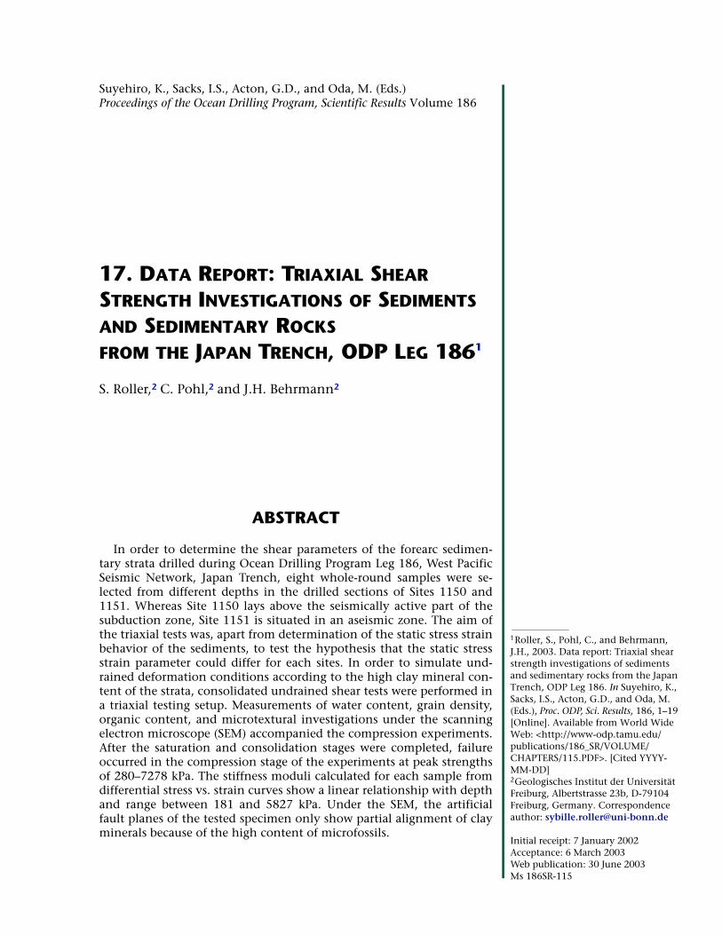
Suyehiro, K., Sacks, I.S., Acton, G.D., and Oda, M. (Eds.)Proceedings of the Ocean Drilling Program, Scientific Results Volume 186

17. DATA REPORT: TRIAXIAL SHEAR STRENGTH INVESTIGATIONS OF SEDIMENTS AND SEDIMENTARY ROCKS FROM THE JAPAN TRENCH, ODP LEG 1861

S. Roller,2 C. Pohl,2 and J.H. Behrmann2

ABSTRACT

In order to determine the shear parameters of the forearc sedimen-tary strata drilled during Ocean Drilling Program Leg 186, West PacificSeismic Network, Japan Trench, eight whole-round samples were se-lected from different depths in the drilled sections of Sites 1150 and1151. Whereas Site 1150 lays above the seismically active part of thesubduction zone, Site 1151 is situated in an aseismic zone. The aim ofthe triaxial tests was, apart from determination of the static stress strainbehavior of the sediments, to test the hypothesis that the static stressstrain parameter could differ for each sites. In order to simulate und-rained deformation conditions according to the high clay mineral con-tent of the strata, consolidated undrained shear tests were performed ina triaxial testing setup. Measurements of water content, grain density,organic content, and microtextural investigations under the scanningelectron microscope (SEM) accompanied the compression experiments.After the saturation and consolidation stages were completed, failureoccurred in the compression stage of the experiments at peak strengthsof 280–7278 kPa. The stiffness moduli calculated for each sample fromdifferential stress vs. strain curves show a linear relationship with depthand range between 181 and 5827 kPa. Under the SEM, the artificialfault planes of the tested specimen only show partial alignment of clayminerals because of the high content of microfossils.

1Roller, S., Pohl, C., and Behrmann, J.H., 2003. Data report: Triaxial shear strength investigations of sediments and sedimentary rocks from the Japan Trench, ODP Leg 186. In Suyehiro, K., Sacks, I.S., Acton, G.D., and Oda, M. (Eds.), Proc. ODP, Sci. Results, 186, 1–19 [Online]. Available from World Wide Web: <http://www-odp.tamu.edu/publications/186_SR/VOLUME/CHAPTERS/115.PDF>. [Cited YYYY-MM-DD]2Geologisches Institut der Universität Freiburg, Albertstrasse 23b, D-79104 Freiburg, Germany. Correspondence author: sybille.roller@uni-bonn.de

Initial receipt: 7 January 2002Acceptance: 6 March 2003Web publication: 30 June 2003Ms 186SR-115

S. ROLLER ET AL.DATA REPORT: TRIAXIAL SHEAR STRENGTH 2

INTRODUCTION

The data presented stem from a suite of geotechnical experimentscarried out on whole-round samples drilled during Ocean Drilling Pro-gram (ODP) Leg 186, West Pacific Seismic Network, Japan Trench. Thescientific objectives of the cruise were the installation of two in situmeasurement devices (seismometers, strainmeter, and tiltmeter) (for de-tails see the Leg 186 Initial Reports volume [Sacks, Suyehiro, Acton, etal., 2000]) in the forearc of the Japan Trench at Sites 1150 and 1151.The measurements may help explain why there are seismic (Site 1150)and aseismic (Site 1151) domains in the forearc. Laboratory triaxial de-formation tests on eight samples from different depths in the twodrilled sections (see Table T1) should provide information on the staticstress strain behavior of the sedimentary rocks of both sites.

Triaxial tests are a useful tool to determine deformation-specificproperties of rocks under realistic conditions (i.e., a cylindrical speci-men is subjected to a confining pressure comparable to the horizontalstress in the Earth’s crust). Vertical stress resulting from lithostatic over-load is simulated by axial piston loading. The vertical load is increaseduntil failure occurs. From the possible types of triaxial tests, the consol-idated undrained (CU) test is considered to be most suitable to simulateabrupt earthquake-induced deformation, a buildup of pore pressure,which results from impeded drainage in the clayey sediments and sedi-mentary rocks. In contrast, the consolidated drained (CD) test permitsthe escape of pore water without an increase of pore pressure. Deforma-tion rates during CD tests are 10 times lower than those of CU tests.

Some samples were cut in several orientations to the artificially gen-erated fault surface and were prepared for the scanning electron micro-scopy (SEM) to investigate the characteristics and development of thepore space with depth, as well as, the orientation and microstructuresof the platy and clayey mineral components on the artificial fault planesurfaces.

METHODS

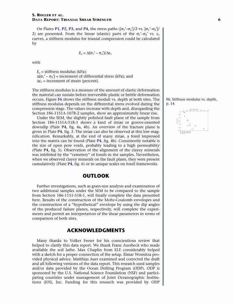
Standard triaxial tests are symmetrical compression tests on cylindri-cal samples, primarily performed to determine the shear strength of amaterial. The experiments were carried out using an ELE Tritest 50setup, with a maximum cell pressure of 1700 kPa and maximum verti-cal load of 7500 N (Fig. F1). The horizontal stresses (σ2 = σ3) are imposedby water pressure; the vertical stress (σ1) is imposed by piston load andwater pressure (σ1 = F/A + σ3, with F = piston load and A = area). The wa-ter used for external and internal application of pressure to the speci-men has to be de-aired to avoid measurement errors due tocompressibility of the gaseous phase. The cylindrical triaxial cell en-closes the specimen, which is installed on the cell base. The cell basecontains the influx to and drainage off the cell and the specimen (Fig.F1). The outlets and inlets are each equipped with electrical sensors andconnected through piping with either hydraulic pumps (water supply)or with measuring devices (volume change unit and pressure gauges).

The tests were carried out according to the instructions and recom-mendations for the determination of shear strength given by the Ger-man Institute for Standardization (DIN 18 137, 1990; see parts 1 and 2)and are characterized by three stages: (1) saturation, (2) consolidation,

T1. Samples, testing program, and test results, p. 15.

F1. Triaxial test setup, p. 9.

Cellpressure

sensor

Drainage-to-volume change

sensor

Pore pressuresensor

Top drainage

Pore flush

Load transducerStrain gauge

Test specimen

S. ROLLER ET AL.DATA REPORT: TRIAXIAL SHEAR STRENGTH 3

and (3) compression. Saturation pore pressure is a kind of passive porepressure induced in the specimen by a hydraulic pump. The pore pres-sure during consolidation and compression stages is defined as backpressure, as it rises in the tested specimen as a reaction to cell pressureand piston load.

Basically, a series of three tests at different confining pressures mustbe conducted to construct the Mohr-Coulomb envelope in the shearstress (τ) vs. normal stress (σn) diagram. Limited sample volume, due tofracturing and required sample size, restricted the number of tests perwhole-round sample to only two at different cell pressures, or even onlyone. This circumstance reduces the accuracy of Mohr-Coulomb enve-lopes and makes determinations of shear parameters less precise.

As mentioned before, failure of the sample is induced by a piston ad-vancing at constant speed (for velocities for each sample see Table T1),causing increasing vertical stress (σ1). The development of the verticalforce is measured by a load transducer. The tests are run until an ulti-mate condition is reached (Head, 1986). Failure criteria can serve boththe peak differential stress, where shear strength of the sample is ex-ceeded, or a limiting strain of 15%–20% for plastically deforming soils.The axial shortening is measured by a strain-gauge sensor (Fig. F1). Dur-ing undrained tests, the drainage system is locked and a pore pressurebuilds up as a result of compression. The vertical load and the displace-ment of the piston are measured by the load transducer and straingauge sensor in time intervals, depending on the amount of change ofthese quantities. Except for the deepest sample from Site 1151, thestrength of which exceeded the limit force of the load transducer unit,all tests were carried out until the failure criteria were reached. Twosamples from Section 186-1151A-84R-2 were analyzed using drainedshear tests because of temporarily defective testing conditions. On theone hand, the stiffness moduli obtained are comparable to those of theundrained tests, but on the other hand, we could not infer the cohesionand the internal angle of friction.

According to the size of the cell’s base, the samples had diameters of35 mm. However, as most of the cores from Site 1150 underwent post-drilling stress relaxation (Figs. F2, F3), in most cases, only cylinderswith diameters of 24 mm could be carved out. Sample preparation in-cluded sawing of the whole-round cores into pieces of required length,which amounted to 2–2.5 times the diameter. With the aid of a hand-operated soil lathe, the samples were cut and rasped into a cylindricalshape with a constant diameter of 35 mm (Head, 1982). Specimens withdiameters <35 mm had to be prepared without the lathe. The top andbottom surfaces of the cylinders had to be cut off evenly and parallel toeach other to avoid strain concentrations at the piston/specimen inter-face (Jaeger and Cook, 1979). The sample preparation had to be donevery carefully to avoid disturbance of texture and cohesion. Before be-ing installed into the cell, the specimen was wrapped in filter-paper sidedrains. Afterward, porous disks were fitted to both ends of the filter-wrapped cylinder before it was inserted into an impermeable rubbermembrane. This drainage assemblage allowed an optimum of waterflux in a vertical as well as horizontal direction and a homogeneous dis-tribution of pore water pressure. With the setup and sample preparationdescribed, a natural-rock surrounding could be roughly modeled. Paral-lel to the preparation of the cylinders, the water content and grain den-sity were determined (Table T1). Porosity data were simply adoptedfrom the shipboard measurements (Sacks, Suyehiro, Acton, et al., 2000).

F2. Postdrilling stress relaxation fracture, p. 10.

Section 186-1151A-51R-1

F3. Relaxation phenomena, p. 11.

S. ROLLER ET AL.DATA REPORT: TRIAXIAL SHEAR STRENGTH 4

After the sample was installed in the cell and connected to the topand base drainage system (Fig. F1), the cell and the connecting pipeswere flooded with de-aired water. The general procedure of a CU test isas follows:

1. A defined and reproducible stress state is established in the spec-imen by saturation and consolidation.

2. The drainage system is closed.3. Vertical load is increased by continuously displacing the piston

downward.

The aim of saturation is to dissolve remaining air in the pore water.Air in the pores corrupts the results of the compression test. To achievesaturation, the cell pressure and the pore pressure are increased simulta-neously. The value of necessary saturation pore pressure depends on theinitial saturation (S0) of the material tested:

S0 = (wρs [1 – n])/(nρw)

where

S0 = initial saturation;w = water content (percent); ρs = grain density (g/cm3); n = porosity (percent); andρw = density of water (g/cm3).

According to DIN 18 137 (1990) part 2, initial saturation S0 between0.65 and 0.9 requires a saturation pore pressure between 200 and 900kPa. In all experiments, cell pressure and saturation pressure (σp) were in-creased incrementally in three steps to avoid damage to the sedimentaryfabric. The amount of water squeezed into the specimen was measuredby the volume change device. A typical pressure-water influx correlationis given in Figure F4. The progress of saturation was controlled by closingthe valve to the volume change device and subsequently raising the cellpressure by up to 10%. When saturation is achieved, the ratio of porepressure change to the cell pressure change must be >0.95. In the clayeysediments and sedimentary rocks tested, the saturation stage lasted anaverage of 72 hr.

After the completion of saturation, the test specimens were consoli-dated. The objective of consolidation is to create a defined equilibriumand isotropic stress state before the specimen is loaded to failure. Evi-dently, the values of consolidation pressure are higher than saturationpressure and are always restricted by the limiting stress value of themeasurement device. The pressures were chosen in intervals approxi-mately proportional to the drilling depth of the sections (for appliedconsolidation pressure values see Table T1). The cell pressure was in-creased, starting from the final cell pressure of the saturation stage,while the formerly applied saturation pore pressure was maintained.Under these isotropic stress conditions and with open drainage, therewas an initial rise in pore pressure followed by a fall due to the dewater-ing of the specimen into the back pressure system. When the back pres-sure and volume change reached a constant value with time, theconsolidation stage was completed. A typical volume change-time cor-relation can be seen in Figure F5, which shows a graph with an initiallysteep slope becoming progressively flatter with time. Consolidation

F4. Saturation data, p. 12.

Time (min)

0 1000 2000 3000 4000 5000

Vol

ume

chan

ge (

mL)

Cel

l pre

ssur

e (k

Pa)

A

B

-2

0

2

4

6

8

10

0

100

200

300

400

500

600

700

F5. Consolidation diagram, p. 13.

Time (min)

Vol

ume

chan

ge (

mL)

4

5

6

7

8

9

0 200 400 600 800 1000 1200 1400 1600 1800

S. ROLLER ET AL.DATA REPORT: TRIAXIAL SHEAR STRENGTH 5

stages usually lasted 25–30 hr. This curve is essential for the calculationof the piston velocity of the compression stage. With the aid of the con-solidation, the empirical equation (DIN 18 137, 1990, part 2; Head,1986) gives the maximum piston velocity for drained tests:

max v = (h × εf)/(15×t100)

where

max v = maximum rate of deformation (mm/min); h = height of sample (mm);εf = estimated strain at failure; andt100 = graphically constructed time at 100% consolidation (min).

The calculated rate is valid for CD tests. For CU tests, however, the rateof deformation should be at least 10 times faster. For our tests, weroughly calculated the rate then compared the latter with the order ofmagnitude recommended in the DIN standard (DIN 18 137, 1990) (de-pending on the degree of plasticity of the tested material), and, based onthe results, determined a rate (Table T1). Additionally, the maximumload capacity of the triaxial testing frame (load transducer limit = 7500N) had to be considered, so lower rates of deformation were chosen fordeeper and, hence, stronger samples. In this context, it is worth men-tioning the advantage of the small-diameter specimens.

To investigate if and how far clay minerals are oriented in the vicin-ity of the artificially induced fracture planes, small cubes of materialwere extracted from Sample 186-1151A-51R-1, 53–63 cm (546 metersbelow seafloor), in different orientations from the deformed cylinder.After freeze-drying, mounting on aluminium tables, and cathodic sput-tering with carbon to make the surface of the subsamples electrocon-ductive, the subsamples were exposed to the electron beam of the SEM.The organic matter content was determined for each tested section asthe weight loss after oxidizing the material at 550°C for 2 hr (followingthe recommendations of DIN 18 121, 1990).

RESULTS

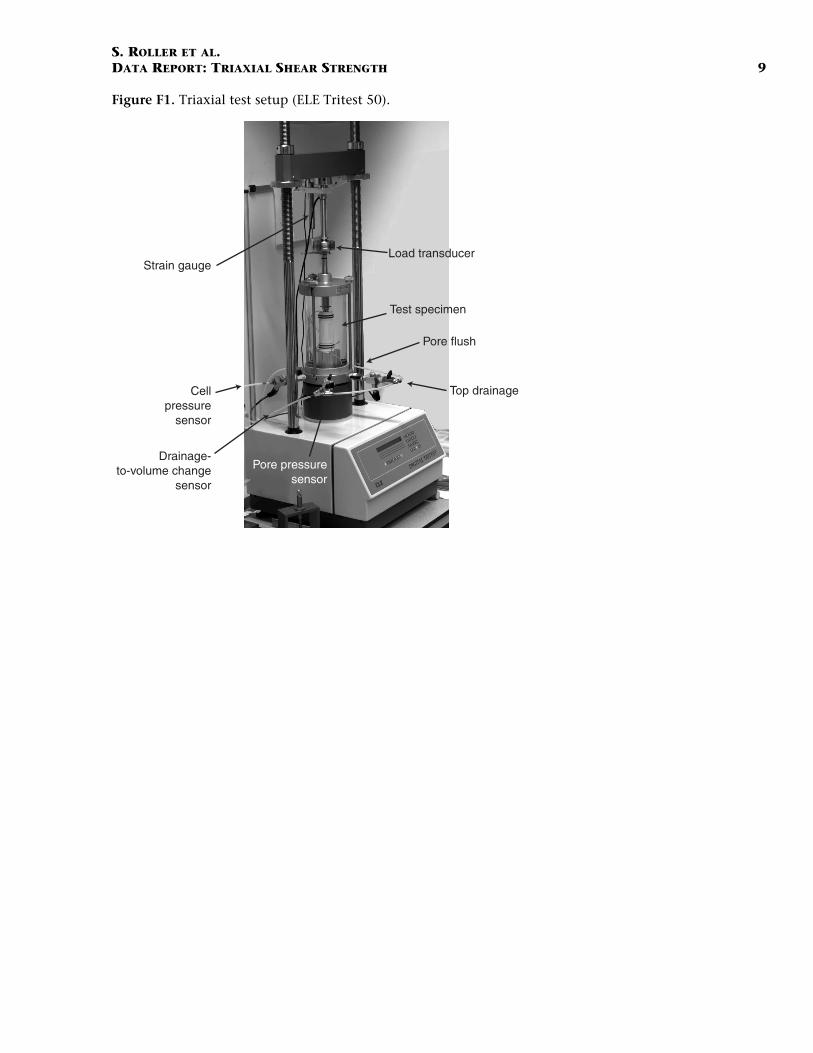
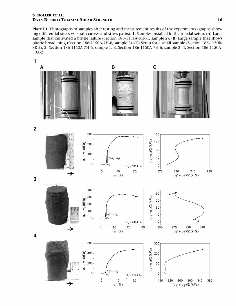
Different modes of failure were observed; most firm and hard sam-ples failed by shear and some of the softer samples showed plasticbroadening (see Plates P1, P2, P3, P4). Different modes of brittle failureoccurred, as there are near-vertical extension fractures, slightly inclinedhybrid-extension shear fractures, and shear fractures. Proof for the real-istic conditions of the triaxial tests is the perfect parallelism of healedoriginal fractures and artificial shear planes. The fact that a new shearplane was generated instead of reactivating a preexisting discontinuity(Plate P3, fig. 1) has an important implication—the inhomogeneitydoes not influence later deformation in terms of being a location of me-chanical weakness. In conclusion, it follows that apart from the need tofind intact parts of the cores for preparation of test specimens, thereseems to be no need for the samples to be free of healed fractures.

For the evaluation of the results, the effective stresses (σ′) have to becalculated, subtracting the measured pore pressure (∆u) from vertical(σ1) and horizontal (σ3) stresses.

P1. Samples after testing in triax-ial setup, p. 16.

0 10 20

180 220 260 300 340 380

σ 1 -

σ3

(kP

a)

(σ1

- σ 3

)/2

(kP

a)

σ 1 -

σ3

(kP

a)

(σ1

- σ 3

)/2

(kP

a)

σ 1 -

σ3

(kP

a)

(σ1

- σ 3

)/2

(kP

a)

0

200

400

600

0

100

200

300

0

100

200

300

400

0

40

80

120

160

0

100

200

300

0

40

80

120

160

ε1 (%) (σ1' + σ3')/2 (kPa)

ε1 (%) (σ1' + σ3')/2 (kPa)

ε1 (%) (σ1' + σ3')/2 (kPa)

0 10 20 30 250 270 290 310

0 10 20 170 190 210 230

Ev = 181 kPa

Ev = 240 kPa

Ev = 276 kPa

∆ (σ1 - σ3)∆ε1

∆(σ1 - σ3)∆ε1

∆(σ1 - σ3)

∆ε1

1

2

3

4

A B C

1cm

1cm1cm

P2. Section 186-1150B-8R-2, p. 17.

∆(σ1 - σ3)

σ 1 -

σ3

(kP

a)σ 1

- σ

3 (k

Pa)

σ 1 -

σ3

(kP

a)σ 1

- σ

3 (k

Pa)

0

1000

2000

0

2000

4000

0

1000

2000

0

1000

2000

3000

ε1 (%)

ε1 (%)

ε1 (%)

ε1 (%)

(σ1' + σ3')/2 (kPa)

(σ1' + σ3')/2 (kPa)

(σ1' + σ3')/2 (kPa)

(σ1' + σ3')/2 (kPa)

0

400

800

0

1000

2000

0

400

800

1200

0

400

800

1200

0 400 800 12000 2 4 6

0 1000 20000 2 4

0 400 800 12000 2 4

0 400 800 12000 2 4

(σ1

- σ 3

)/2

(kP

a)(σ

1 -

σ 3)/

2 (k

Pa)

(σ1

- σ 3

)/2

(kP

a)(σ

1 -

σ 3)/

2 (k

Pa)

Ev = 1789 kPa

Ev = 3472 kPa

Ev = 2763 kPa

Ev = 2348 kPa

∆(σ1 - σ3)

∆(σ1 - σ3)

∆(σ1 - σ3)

∆ε1

∆ε1

∆ε1

∆ε1

1

2

3

4

P3. Section 186-1151A-51R-1, p. 18.

Ev = 1103 kPa

Ev = 1324 kPa

Ev = 1119 kPa

Ev = 1854 kPa

σ 1 -

σ3

(kP

a)σ 1

- σ

3 (k

Pa)

σ 1 -

σ3

(kP

a)σ 1

- σ

3 (k

Pa)

∆(σ1 - σ3)

∆ε1

∆(σ1 - σ3)

∆ε1

∆(σ1 - σ3)

∆ε1

∆(σ1 - σ3)

∆ε1

(σ1

- σ 3

)/2

(kP

a)(σ

1 -

σ 3)/

2 (k

Pa)

(σ1

- σ 3

)/2

(kP

a)(σ

1 -

σ 3)/

2 (k

Pa)

0

2000

4000

0

400

800

1200

1600

0

1000

2000

0

1000

2000

3000

0

400

800

0

400

800

1200

0

1000

2000

0

400

800

1200

1600

(σ1' + σ3')/2 (kPa)

(σ1' + σ3')/2 (kPa)

(σ1' + σ3')/2 (kPa)

(σ1' + σ3')/2 (kPa)

ε1 (%)

ε1 (%)

ε1 (%)

ε1 (%)100 300 500 7000 2 4

400 600 800 1000 12000 2 4 6

200 600 1000 1400 18000 2 4 6 8 10 12 14

0 4 8 12 1000 2000 3000

1

2

3

4

P4. Section 186-1151A-107R-2, p. 19.

500 µm

100 µm

20 µm 2 µm

500 nm

1 cm

σ 1 -

σ3

(kP

a)σ 1

- σ

3 (k

Pa)

(σ1

- σ 3

)/2

(kP

a)(σ

1 -

σ 3)/

2 (k

Pa)

0

2000

4000

6000

0

1000

2000

3000

0

2000

4000

6000

8000

0

1000

2000

3000

4000

ε1 (%)

ε1 (%)

(σ1' + σ3')/2 (kPa)

(σ1' + σ3')/2 (kPa)

0 1 2 3 4 0 1000 2000 3000

0 1 2 3 0 2000 4000

Coefficients:b[0] = -6504.03b[1] = 5826.70r2 = 0.99

∆(σ1 - σ3)

∆ε1

∆(σ1 - σ3)

∆ε1Coefficients:b[0] = -4607.99b[1] = 5761.75r2 = 0.99

1

2

3A

5 6

B4

S. ROLLER ET AL.DATA REPORT: TRIAXIAL SHEAR STRENGTH 6

On Plates P1, P2, P3, and P4, the stress paths ([σ1′–σ3′]/2 vs. [σ1′–σ3′]/2) are presented. From the linear (elastic) parts of the σ1′–σ3′ vs. ε1

curves, a stiffness modulus for triaxial compression could be calculatedby

Ev = ∆(σ1′ – σ3′)/∆ε1

with

Ev = stiffness modulus (kPa);∆(σ1′ – σ3′) = increment of differential stress (kPa); and∆ε1 = increment of strain (percent).

The stiffness modulus is a measure of the amount of elastic deformationthe material can sustain before irreversible plastic or brittle deformationoccurs. Figure F6 shows the stiffness moduli vs. depth at both sites. Thestiffness modulus depends on the differential stress evolved during thecompression stage. The values increase with depth and, disregarding theSection 186-1151A-107R-2 samples, show an approximately linear rise.

Under the SEM, the slightly polished fault plane of the sample fromSection 186-1151A-51R-1 shows a kind of striae or groove-orienteddowndip (Plate P4, fig. 4a, 4b). An overview of the fracture plane isgiven in Plate P4, fig. 3. The striae can also be observed at this low mag-nification. Remarkably, at the end of many striae, a fossil impressedinto the matrix can be found (Plate P4, fig. 4b). Consistently notable isthe size of open pore voids, probably leading to a high permeability(Plate P4, fig. 5). Observation of the alignment of the clayey mineralswas inhibited by the “cemetery” of fossils in the samples. Nevertheless,when we observed clayey minerals on the fault plane, they were presentcumulatively (Plate P4, fig. 6) or in unique scales on fossil frameworks.

OUTLOOK

Further investigations, such as grain-size analysis and examination oftwo additional samples under the SEM to be compared to the samplefrom Section 186-1151-51R-1, will finally complete the data presentedhere. Results of the construction of the Mohr-Coulomb envelopes andthe construction of a “hypothetical” envelope by using the dip anglesof the produced failure planes, respectively, will complete the experi-ments and permit an interpretation of the shear parameters in terms ofcomparison of both sites.

ACKNOWLEDGMENTS

Many thanks to Volker Feeser for his conscientious review thathelped to clarify this data report. We thank Franz Auerbeck who madeavailable the soil lathe. Max Chaplin from ELE considerably helpedwith a sketch for a proper connection of the setup. Elmar Wosnitza pro-vided physical advice. Matthias Auer examined and corrected the draftand all following versions of the data report. This research used samplesand/or data provided by the Ocean Drilling Program (ODP). ODP issponsored by the U.S. National Science Foundation (NSF) and partici-pating countries under management of Joint Oceanographic Institu-tions (JOI), Inc. Funding for this research was provided by ODP

F6. Stiffness modulus vs. depth, p. 14.

Stiffness modulus (kPa)

0 1000 2000 3000 4000 5000 6000 7000

Dep

th (

mbs

f)

Site 1150 - large samplesSite 1150 - small samplesSite 1151

1200

1000

800

600

400

200

0

S. ROLLER ET AL.DATA REPORT: TRIAXIAL SHEAR STRENGTH 7

Germany. Many thanks to ODP for generously providing the large vol-ume of samples for our tests.

S. ROLLER ET AL.DATA REPORT: TRIAXIAL SHEAR STRENGTH 8

REFERENCES

DIN 18 137, 1990. (German Standard) Testing Procedures and Apparatus: Triaxial Test,Part 2: Berlin (Deutsches Institut für Normung).

DIN 18 121, 1976. (German Standard) Determination of Water Content by Oven Drying:Berlin (Deutsches Institut für Normung).

Head, K.H., 1982. Manual of Soil Laboratory Testing (Vol. 2): Permeability, Shear Strengthand Compressibility Tests: New York (Halsted Press/Wiley).

————, 1986. Manual of Soil Laboratory Testing (Vol. 3): Effective Stress Tests: NewYork (Halsted Press/Wiley).

Jaeger, J.C., and Cook, N.G.W., 1979. Fundamentals of Rock Mechanics (3rd ed.): NewYork (Chapman and Hall).

Sacks, I.S., Suyehiro, K., Acton, G.D., et al., 2000. Proc. ODP, Init. Repts., 186 [CD-ROM]. Available from: Ocean Drilling Program, Texas A&M University, College Sta-tion TX 77845-9547, USA.

S. ROLLER ET AL.DATA REPORT: TRIAXIAL SHEAR STRENGTH 9

Figure F1. Triaxial test setup (ELE Tritest 50).

Cellpressure

sensor

Drainage-to-volume change

sensor

Pore pressuresensor

Top drainage

Pore flush

Load transducerStrain gauge

Test specimen

S. ROLLER ET AL.DATA REPORT: TRIAXIAL SHEAR STRENGTH 10

Figure F2. Section 186-1151A-51R-1 shows a large fracture as a result of postdrilling stress relaxation.

Section 186-1151A-51R-1

S. ROLLER ET AL.DATA REPORT: TRIAXIAL SHEAR STRENGTH 11

Figure F3. Section 186-1150B-21R-1 relaxation phenomena.

S. ROLLER ET AL.DATA REPORT: TRIAXIAL SHEAR STRENGTH 12

Figure F4. Saturation data (sample 1, Section 186-1151A-51R-1). A. Diagram shows the rise of cell pressurein three steps vs. time. B. Diagram as a result of parallel rise in cell pressure and pore pressure. The volumechange device shows the flux of water into the sample.

Time (min)

0 1000 2000 3000 4000 5000

Vol

ume

chan

ge (

mL)

Cel

l pre

ssur

e (k

Pa)

A

B

-2

0

2

4

6

8

10

0

100

200

300

400

500

600

700

S. ROLLER ET AL.DATA REPORT: TRIAXIAL SHEAR STRENGTH 13

Figure F5. Consolidation diagram (sample 2, Section 186-1150A-7H-6).

Time (min)

Vol

ume

chan

ge (

mL)

4

5

6

7

8

9

0 200 400 600 800 1000 1200 1400 1600 1800

S. ROLLER ET AL.DATA REPORT: TRIAXIAL SHEAR STRENGTH 14

Figure F6. Stiffness modulus vs. depth.

Stiffness modulus (kPa)

0 1000 2000 3000 4000 5000 6000 7000

Dep

th (

mbs

f)

Site 1150 - large samplesSite 1150 - small samplesSite 1151

1200

1000

800

600

400

200

0

S. RO

LL

ER

ET A

L.D

AT

A R

EP

OR

T: TR

IAX

IAL S

HE

AR

ST

RE

NG

TH

1

5

Table

Note: C

Core,section est

Height (mm)

Diameter (mm)

Grain density (g/cm3)

Watercontent

(%)

Organic mattercontent

(%)

Saturation pressure

(kPa)

Consolidation pressure

(kPa)

Rate of deformation (mm/min)

Yield strength maximum

(σ1 – σ3) (kPa)

Stiffness modulusEv (kPa)

186-11507H-6 CU 73.3 35 2.5 57 4.8 480 630 0.06 280 181

CU 78.5 35 55 530 800 0.06 340 24030X-2 CU 81 35 2.33 88 5.7 200 400 0.03 485 276

186-11508R-2 CU 51.8 24 2.18 68 5.9 200 250 0.01 1891 178921R-1 CU 81.2 35 2.38 37 5.3 750 900 0.008 3912 347242R-5 CU 47.5 24 2.27 35 5 250 300 0.008 2211 2763

CU 46.3 24 35 250 355 0.008 2418 2348

186-115151R-1 CU 85.2 35 2.18 76 6.5 600 800 0.01 1371 1103

CU 72.5 35 79 600 1050 0.01 2045 132484R-2 CD 82 35 2.23 49 5.2 900 1300 0.01 5558 1119

CD 82 35 53 900 1545 0.01 4682 1854107R-2 CU 85.7 35 2.33 41 4.8 900 1000 0.002 6326 5827

CU 85.9 35 37 900 960 0.002 7278 5762

T1. List of samples, testing programs, and test results.

U = consolidated undrained, CD = consolidated drained.

Depth (mbsf) Lithology Induration

Sample number T

A-63 Glass diatom spicule-bearing silty clay Soft 1

2272 Diatom spicule glass-bearing clay Soft 1

B-769 Diatomaceous silty clay Hard 1893 Diatom glass quartz-bearing silty clay Hard 1

1101 Diatom glass-bearing silty clay Hard 12

A-546 Spicule-bearing diatomaceous silty clay Firm 1

2864 Glass diatom spicule-bearing silty clay Firm/hard 1

21087 Glass and spicule-bearing silty clay Hard 1

2

S. ROLLER ET AL.DATA REPORT: TRIAXIAL SHEAR STRENGTH 16

Plate P1. Photographs of samples after testing and measurement results of the experiments (graphs show-ing differential stress vs. strain curves and stress paths). 1. Samples installed in the triaxial setup. (A) Largesample that cultivated a brittle failure (Section 186-1151A-51R-1, sample 2). (B) Large sample that showsplastic broadening (Section 186-1150A-7H-6, sample 2). (C) Setup for a small sample (Section 186-1150B-8R-2). 2. Section 186-1150A-7H-6, sample 1. 3. Section 186-1150A-7H-6, sample 2. 4. Section 186-1150A-30X-2.

0 10 20

180 220 260 300 340 380

σ 1 -

σ3

(kP

a)

(σ1

- σ 3

)/2

(kP

a)

σ 1 -

σ3

(kP

a)

(σ1

- σ 3

)/2

(kP

a)

σ 1 -

σ3

(kP

a)

(σ1

- σ 3

)/2

(kP

a)

0

200

400

600

0

100

200

300

0

100

200

300

400

0

40

80

120

160

0

100

200

300

0

40

80

120

160

ε1 (%) (σ1' + σ3')/2 (kPa)

ε1 (%) (σ1' + σ3')/2 (kPa)

ε1 (%) (σ1' + σ3')/2 (kPa)

0 10 20 30 250 270 290 310

0 10 20 170 190 210 230

Ev = 181 kPa

Ev = 240 kPa

Ev = 276 kPa

∆ (σ1 - σ3)∆ε1

∆(σ1 - σ3)∆ε1

∆(σ1 - σ3)

∆ε1

1

2

3

4

A B C

1cm

1cm1cm

S. ROLLER ET AL.DATA REPORT: TRIAXIAL SHEAR STRENGTH 17

Plate P2. Photographs of samples after testing and measurement results of the experiments (graphs show-ing differential stress vs. strain curves and stress paths). 1. Section 186-1150B-8R-2. 2. Section 186-1150B-21R-1. 3. Section 186-1150B-42R-5, sample 1. 4. Section 186-1150B-42R-5, sample 2.

∆(σ1 - σ3)

σ 1 -

σ3

(kP

a)σ 1

- σ

3 (k

Pa)

σ 1 -

σ3

(kP

a)σ 1

- σ

3 (k

Pa)

0

1000

2000

0

2000

4000

0

1000

2000

0

1000

2000

3000

ε1 (%)

ε1 (%)

ε1 (%)

ε1 (%)

(σ1' + σ3')/2 (kPa)

(σ1' + σ3')/2 (kPa)

(σ1' + σ3')/2 (kPa)

(σ1' + σ3')/2 (kPa)

0

400

800

0

1000

2000

0

400

800

1200

0

400

800

1200

0 400 800 12000 2 4 6

0 1000 20000 2 4

0 400 800 12000 2 4

0 400 800 12000 2 4

(σ1

- σ 3

)/2

(kP

a)(σ

1 -

σ 3)/

2 (k

Pa)

(σ1

- σ 3

)/2

(kP

a)(σ

1 -

σ 3)/

2 (k

Pa)

Ev = 1789 kPa

Ev = 3472 kPa

Ev = 2763 kPa

Ev = 2348 kPa

∆(σ1 - σ3)

∆(σ1 - σ3)

∆(σ1 - σ3)

∆ε1

∆ε1

∆ε1

∆ε1

1

2

3

4

S. ROLLER ET AL.DATA REPORT: TRIAXIAL SHEAR STRENGTH 18

Plate P3. Photographs of samples after testing and measurement results of the experiments (graphs show-ing differential stress vs. strain curves and stress paths). 1. Section 186-1151A-51R-1, sample 1. 2. Section186-1151A-51R-1, sample 2. 3. Section 186-1151A-84R-2, drained experiment. Photograph shows samplewith filter paper. 4. Section 186-1151A-84R-2, drained experiment. Photograph shows sample with filterpaper.

Ev = 1103 kPa

Ev = 1324 kPa

Ev = 1119 kPa

Ev = 1854 kPa

σ 1 -

σ3

(kP

a)σ 1

- σ

3 (k

Pa)

σ 1 -

σ3

(kP

a)σ 1

- σ

3 (k

Pa)

∆(σ1 - σ3)

∆ε1

∆(σ1 - σ3)

∆ε1

∆(σ1 - σ3)

∆ε1

∆(σ1 - σ3)

∆ε1

(σ1

- σ 3

)/2

(kP

a)(σ

1 -

σ 3)/

2 (k

Pa)

(σ1

- σ 3

)/2

(kP

a)(σ

1 -

σ 3)/

2 (k

Pa)

0

2000

4000

0

400

800

1200

1600

0

1000

2000

0

1000

2000

3000

0

400

800

0

400

800

1200

0

1000

2000

0

400

800

1200

1600

(σ1' + σ3')/2 (kPa)

(σ1' + σ3')/2 (kPa)

(σ1' + σ3')/2 (kPa)

(σ1' + σ3')/2 (kPa)

ε1 (%)

ε1 (%)

ε1 (%)

ε1 (%)100 300 500 7000 2 4

400 600 800 1000 12000 2 4 6

200 600 1000 1400 18000 2 4 6 8 10 12 14

0 4 8 12 1000 2000 3000

1

2

3

4

S. ROLLER ET AL.DATA REPORT: TRIAXIAL SHEAR STRENGTH 19

Plate P4. Photographs of samples after testing and measurement results of the experiments (graphs show-ing differential stress vs. strain curves and stress paths). 1. Section 186-1151A-107R-2, sample 1. 2. Section186-1151A-107R-2, sample 2. 3. Section 186-1151A-51R-1, sample 1. View of the fracture plane after triaxialtest. 4. Section 186-1151A-51R-1, sample 1, SEM picture. (A) Shows striae oriented downdip (BSE mode)with (B) detail of (A) showing fossil remains impressed into the matrix at the end of the striae. 5. Section186-1151A-51R-1, sample 1, SEM picture. Example of the open pore voids between the fossils. 6. Section186-1151A-51R-1, sample 1, SEM picture. Accumulation of clay minerals. Detail shows a single platelet.

500 µm

100 µm

20 µm 2 µm

500 nm

1 cm

σ 1 -

σ3

(kP

a)σ 1

- σ

3 (k

Pa)

(σ1

- σ 3

)/2

(kP

a)(σ

1 -

σ 3)/

2 (k

Pa)

0

2000

4000

6000

0

1000

2000

3000

0

2000

4000

6000

8000

0

1000

2000

3000

4000

ε1 (%)

ε1 (%)

(σ1' + σ3')/2 (kPa)

(σ1' + σ3')/2 (kPa)

0 1 2 3 4 0 1000 2000 3000

0 1 2 3 0 2000 4000

Coefficients:b[0] = -6504.03b[1] = 5826.70r2 = 0.99

∆(σ1 - σ3)

∆ε1

∆(σ1 - σ3)

∆ε1Coefficients:b[0] = -4607.99b[1] = 5761.75r2 = 0.99

1

2

3A

5 6

B4