Data Rate Performance Gains in UMTS Evolution at the ...
109
b Data Rate Performance Gains in UMTS Evolution at the Cellular Level Gonçalo Nuno Coelho e Ferraz de Carvalho Dissertation submitted for obtaining the degree of Master in Electrical and Computer Engineering Jury Supervisor: Prof. Luís M. Correia Co-Supervisor: Mr. David Antunes President: Prof. José Bioucas Dias Member: Prof. António Rodrigues October 2009
Transcript of Data Rate Performance Gains in UMTS Evolution at the ...

b
Data Rate Performance Gains in UMTS Evolution at the
Cellular Level
Gonçalo Nuno Coelho e Ferraz de Carvalho
Dissertation submitted for obtaining the degree of
Master in Electrical and Computer Engineering
Jury
Supervisor: Prof. Luís M. Correia
Co-Supervisor: Mr. David Antunes
President: Prof. José Bioucas Dias
Member: Prof. António Rodrigues
October 2009

ii

To my family
iii

iv

Acknowledgements
Acknowledgements First of all, I would like to thank Professor Luís Correia for giving me the opportunity to write this
thesis, and for the constant knowledge and experience sharing. I am thankful for his orientation,
availability, constant support and advising, which were key factors to finish the work with the
demanded and desired quality.
To Optimus, especially to David Antunes and Luís Santo, for all the suggestions, technical support
and for having the time to answer all my doubts. I also would like to thank the opportunity to carry out
measurements in the Optimus network, which allowed me to improve my technical knowledge.
To Daniel Sebastião, for his availability to help me with Microsoft Access software.
I also want to thank my colleagues from RF2 Lab, Nuno Jacinto and João Araújo, for their friendship,
suggestions and constructive critics. Without their good company and support, this journey would have
been much harder.
To my girlfriend Joana, for her love, friendship, encouragement, dedication and understanding
throughout the years.
To my friends from Instituto Superior Técnico, for all the moments spent during the academic life. A
special thank to my futsal team mates, for all their fellowship.
To my great friends from ‘Os Cariocas’, for all their support and friendship since our childhood.
Finally, I would to thank my family, especially my parents and siblings, for their unconditional support,
patience, love and care, which are of vital importance to me.
v

vi

Abstract
Abstract The main purpose of this thesis was to analyse UMTS/HSPA+ performance at the cellular level. For
this purpose, measurements were performed in a single user scenario. The behaviour of some
performance parameters was studied, using several settings and under different radio channel
conditions. The comparison between the measured and theoretical data was done, pointing out
explanations for the deviations shown in some cases. In downlink, the highest measured throughput
was 16.3 and 12.6 Mbps, considering instantaneous and average value, respectively. It was confirmed
that, given the same radio channel conditions, the increase of available power does not necessarily
imply the achievement of a better performance. In uplink, the greatest instantaneous throughput was
5.32 Mbps, while the maximum average value was 4.27 Mbps.
Keywords UMTS, HSPA+, Performance, Throughput, Measurements.
vii

viii
Resumo
Resumo O principal objectivo desta tese foi estudar o desempenho do sistema UMTS/HSPA+ a nível celular.
Para tal, foram realizadas medidas num cenário de monoutilizador, tendo sido estudado o
comportamento de alguns parâmetros que medem o desempenho do sistema, usando várias
configurações e com diferentes condições de canal. Foi feita a comparação entre os resultados
medidos e teóricos, e procurou-se encontrar explicações para as disparidades encontradas em
alguns casos. No sentido descendente, o maior débito binário medido foi 16,3 e 12,6 Mbps,
considerando valor instantâneo e médio, respectivamente. Demonstrou-se que, nas mesmas
condições de canal, um aumento de potência disponível não implica necessariamente que se obtenha
uma melhor performance. No sentido ascendente, o débito binário instantâneo máximo medido foi de
5,32 Mbps, sendo que 4,27 Mbps foi o maior valor médio.
Palavras-chave UMTS, HSPA+, Desempenho, Débito Binário, Medidas.

Table of Contents
Table of Contents Acknowledgements .................................................................................. v
Abstract .................................................................................................. vii
Resumo .................................................................................................. viii
Table of Contents .................................................................................... ix
List of Figures .......................................................................................... xi
List of Tables .......................................................................................... xv
List of Acronyms .................................................................................... xvi
List of Symbols ...................................................................................... xix
List of Software ...................................................................................... xxi
1 Introduction .................................................................................... 1
2 Basic Concepts ............................................................................. 5
2.1 UMTS/HSPA ............................................................................................ 6
2.1.1 Network Architecture ............................................................................................. 6
2.1.2 Radio Interface ...................................................................................................... 7
2.1.3 Coverage and Capacity ......................................................................................... 9
2.2 HSPA+ ................................................................................................... 14
2.3 Comparison between HSPA+ and LTE ................................................. 18
2.4 Services and Applications...................................................................... 19
3 Models ......................................................................................... 21
3.1 HSPA+ DL ............................................................................................. 22
ix

x
3.2 HSPA+ UL ............................................................................................. 27
3.3 Assessment ........................................................................................... 28
4 Results Analysis .......................................................................... 31
4.1 Measurements Scenario ........................................................................ 32
4.2 HSPA+ DL ............................................................................................. 33
4.2.1 HS-DSCH Throughput ......................................................................................... 33
4.2.2 CPICH Ec/N0 ........................................................................................................ 44
4.2.3 CQI ...................................................................................................................... 46
4.2.4 Modulation Ratio .................................................................................................. 50
4.2.5 HS-PDSCH Codes............................................................................................... 53
4.2.6 HS-DSCH BLER .................................................................................................. 55
4.3 HSPA+ UL ............................................................................................. 58
4.3.1 E-DCH Throughput .............................................................................................. 58
4.3.2 MT Transmit Power ............................................................................................. 61
4.3.3 E-DCH BLER ....................................................................................................... 63
5 Conclusions ................................................................................. 65
Annex A – MIMO .................................................................................... 69
Annex B – Link Budget ........................................................................... 72
Annex C – HSPA+ DL Additional Results .............................................. 75
References ............................................................................................. 85

List of Figures
List of Figures
Figure 1.1. Peak data rate evolution of 3GPP technologies (adapted from [HoTo09]). ........................... 3
Figure 1.2. Global cellular technology market (extracted from [3GAM09]). ............................................. 3
Figure 2.1. UMTS network architecture (extracted from [HoTo04]). ........................................................ 6
Figure 2.2. HSDPA data rate as function of the average HS-DSCH SINR (extracted from [Pede05]). ..................................................................................................................... 11
Figure 2.3. HSUPA throughput in Vehicular A at 30 km/h, without power control (extracted from [HoTo06]). ..................................................................................................................... 13
Figure 2.4. The 90th percentile throughput for HOM and MIMO (extracted from [BEGG08]). ............... 15
Figure 2.5. Throughput as a function of Ec/N0 for UL HOM (extracted from [PWST07]). ...................... 15
Figure 3.1. HSPA+ DL power scheme. .................................................................................................. 23
Figure 3.2. CQI as a function of HS-DSCH SINR. ................................................................................. 24
Figure 3.3. BLER as a function of SINR on HS-DSCH, considering different CQI values. .................... 27
Figure 4.1. Node B and measurements’ locations view (extracted from [GoEa09]). ............................. 32
Figure 4.2. Theoretical and measured HS-DSCH throughputs as a function of CPICH RSCP using both MTs, with ........................................................................... 34 .dBm45=Tx
BSP
Figure 4.3. Theoretical and measured HS-DSCH throughputs as a function of CPICH RSCP for both MTs, with ..................................................................................... 35 .dBm43=Tx
BSP
Figure 4.4. Theoretical and measured HS-DSCH throughputs as a function of CPICH RSCP for both MTs, with ..................................................................................... 35 .dBm41=Tx
BSP
Figure 4.5. Theoretical and measured HS-DSCH throughputs as a function of CPICH RSCP for the category 14 MT, considering different power configurations. ................................. 36
Figure 4.6. Theoretical and measured HS-DSCH throughputs as a function of CPICH RSCP for the category 8 MT, considering different power configurations. ................................... 36
Figure 4.7. HS-DSCH throughput as a function of CPICH RSCP for the category 14 MT with considering all performed measurements. ......................................... 37 dBm,45=Tx
BSP
Figure 4.8. Theoretical and measured HS-DSCH throughputs as a function of CPICH Ec/N0 using both MTs, with ........................................................................... 38 .dBm45=Tx
BSP
Figure 4.9. Theoretical and measured HS-DSCH throughputs as a function of CPICH Ec/N0 for both MTs, with ..................................................................................... 38 .dBm43=Tx
BSP
Figure 4.10. Theoretical and measured HS-DSCH throughputs as a function of CPICH Ec/N0 for both MTs, with ..................................................................................... 39 .dBm41=Tx
BSP
Figure 4.11. Theoretical and measured HS-DSCH throughputs as a function of CPICH Ec/N0 for the category 14 MT, considering different power configurations. ................................. 39
Figure 4.12. Theoretical and measured HS-DSCH throughputs as a function of CPICH Ec/N0 for the category 8 MT, considering different power configurations. ................................... 40
Figure 4.13. HS-DSCH throughput as a function of CPICH Ec/N0 for the category 14 MT with
xi

dBm,45=TxBSP considering all performed measurements. ......................................... 40
Figure 4.14. Theoretical and measured HS-DSCH throughputs as a function of CQI for both MTs, with ............................................................................................. 41 .dBm45=Tx
BSP
Figure 4.15. Theoretical and measured HS-DSCH throughputs as a function of CQI for both MTs, with ............................................................................................. 42 .dBm43=Tx
BSP
Figure 4.16. Theoretical and measured HS-DSCH throughputs as a function of CQI for both MTs, with ............................................................................................. 42 .dBm41=Tx
BSP
Figure 4.17. Theoretical and measured HS-DSCH throughputs as a function of CQI for the category 14 MT, considering different power configurations. ....................................... 43
Figure 4.18. Theoretical and measured HS-DSCH throughputs as a function of CQI for the category 8 MT, considering different power configurations. ......................................... 43
Figure 4.19. HS-DSCH throughput as a function of CQI for the category 14 MT with considering all measured data. ........................................................... 43 dBm,45=Tx
BSP
Figure 4.20. Theoretical and measured CPICH Ec/N0 as a function of CPICH RSCP for the category 14 MT, considering different power configurations. ....................................... 44
Figure 4.21. Theoretical and measured CPICH Ec/N0 as a function of CPICH RSCP for the category 8 MT, considering different power configurations. ......................................... 45
Figure 4.22. CPICH Ec/N0 as a function of CPICH RSCP for the category 14 MT with considering all measured data. ........................................................... 45 dBm,45=Tx
BSP
Figure 4.23. Measured CPICH Ec/N0 as a function of CPICH RSCP using the category 14 MT with considering situations with and without HSPA+ DL activity. ........ 46 dBm,45=Tx
BSP
Figure 4.24. Theoretical and measured CQIs as a function of CPICH Ec/N0 for both MTs, with ............................................................................................................. 47 .dBm45=Tx
BSP
Figure 4.25. Theoretical and measured CQIs as a function of CPICH Ec/N0 for both MTs, with ............................................................................................................. 48 .dBm43=Tx
BSP
Figure 4.26. Theoretical and measured CQIs as a function of CPICH Ec/N0 for both MTs, with ............................................................................................................. 48 .dBm41=Tx
BSP
Figure 4.27. Theoretical and measured CQIs as a function of CPICH Ec/N0 for the category 14 MT, considering different power configurations. ........................................................... 48
Figure 4.28. Theoretical and measured CQIs as a function of CPICH Ec/N0 for the category 8 MT, considering different power configurations. ........................................................... 49
Figure 4.29. CQI as a function of CPICH Ec/N0 for the category 14 MT with considering all measured data. ..................................................................................... 49
dBm,45=TxBSP
Figure 4.30. Theoretical and measured modulation ratios as a function of CQI with using the category 8 MT. ..................................................................... 50 dBm,45=Tx
BSP
Figure 4.31. Theoretical and measured modulation ratios as a function of CQI with using the category 14 MT. ................................................................... 50 dBm,45=Tx
BSP
Figure 4.32. Theoretical and measured modulation ratios as a function of CPICH RSCP with using the category 8 MT. ..................................................................... 51 dBm,45=Tx
BSP
Figure 4.33. Theoretical and measured modulation ratios as a function of CPICH RSCP with using the category 14 MT. ................................................................... 52 dBm,45=Tx
BSP
Figure 4.34. Theoretical and measured modulation ratios as a function of CPICH Ec/N0 with
xii
dBm,45=TxBSP using the category 8 MT. ..................................................................... 52
Figure 4.35. Theoretical and measured modulation ratios as a function of CPICH Ec/N0 with using the category 14 MT. ................................................................... 53 dBm,45=Tx
BSP
Figure 4.36. Number of HS-PDSCH codes as a function of CQI with using the category 8 MT, considering theoretical and measured data. ....................................... 53
dBm,45=TxBSP
Figure 4.37. Number of HS-PDSCH codes as a function of CQI with using the category 14 MT, considering theoretical and measured data. ..................................... 54
dBm,45=TxBSP
Figure 4.38. Measured HS-PDSCH code usage as a function of CPICH RSCP with considering the category 8 MT. ........................................................... 54 dBm,45=Tx
BSP
Figure 4.39. Measured HS-PDSCH code usage as a function of CPICH RSCP with considering the category 14 MT. ......................................................... 55 dBm,45=Tx
BSP
Figure 4.40. Theoretical HS-DSCH BLER as a function of CPICH RSCP with CQI = 20 and α = 0.8, for different power configurations. ......................................................................... 56
Figure 4.41. Measured HS-DSCH BLER 1st as a function of CPICH RSCP with different power configurations, using the category 14 MT. .................................................................... 56
Figure 4.42. Theoretical HS-DSCH BLER as a function of CPICH Ec/N0 with CQI = 20 and α = 0.8, for different power configurations. ......................................................................... 57
Figure 4.43. Measured HS-DSCH BLER 1st as a function of CPICH Ec/N0 for different power configurations, using the category 14 MT. .................................................................... 57
Figure 4.44. Measured HS-DSCH BLER 1st as a function of CQI for different power configurations, using the category 14 MT. .................................................................... 58
Figure 4.45. Theoretical and measured E-DCH throughputs as a function of CPICH RSCP, considering both TTIs. .................................................................................................. 59
Figure 4.46. Measured E-DCH throughput as a function of CPICH RSCP with 10 ms TTI. .................. 59
Figure 4.47. Theoretical E-DCH throughput as a function of CPICH RSCP with 10 ms TTI. ................ 59
Figure 4.48. Measured E-DCH throughput as a function of CPICH RSCP with 2 ms TTI. .................... 60
Figure 4.49. Theoretical E-DCH throughput as a function of CPICH RSCP with 2 ms TTI. .................. 60
Figure 4.50. Theoretical and measured MT transmit powers as a function of CPICH RSCP, considering both TTIs. .................................................................................................. 61
Figure 4.51. MT transmit power as a function of CPICH RSCP with 10 ms TTI. ................................... 62
Figure 4.52. MT transmit power as a function of CPICH RSCP with 2 ms TTI. ..................................... 62
Figure 4.53. Measured E-DCH BLER 1st as a function of CPICH RSCP, considering both TTIs. ......... 63 Figure A.1. MIMO scheme (extracted from [Maćk07]). .......................................................................... 69
Figure C.1. Theoretical and measured modulation ratios as a function of CPICH RSCP for the category 8 MT, with ............................................................................. 75 .dBm43=Tx
BSP
Figure C.2. Theoretical and measured modulation ratios as a function of CPICH RSCP for the category 8 MT, with ............................................................................. 75 .dBm41=Tx
BSP
Figure C.3. Theoretical and measured modulation ratios as a function of CPICH RSCP for the category 14 MT, with .......................................................................... 76 .dBm43=Tx
BSP
Figure C.4. Theoretical and measured modulation ratios as a function of CPICH RSCP for the
xiii
category 14 MT, with ........................................................................... 76 .dBm41=TxBSP
Figure C.5. Theoretical and measured modulation ratios as a function of CPICH Ec/N0 for the category 8 MT, with ............................................................................. 77 .dBm43=Tx
BSP
Figure C.6. Theoretical and measured modulation ratios as a function of CPICH Ec/N0 for the category 8 MT, with ............................................................................. 77 .dBm41=Tx
BSP
Figure C.7. Theoretical and measured modulation ratios as a function of CPICH Ec/N0 for the category 14 MT, with .......................................................................... 77 .dBm43=Tx
BSP
Figure C.8. Theoretical and measured modulation ratios as a function of CPICH Ec/N0 for the category 14 MT, with ........................................................................... 78 .dBm41=Tx
BSP
Figure C.9. Theoretical and measured modulation ratios as a function of CQI for the category 8 MT, with .............................................................................................. 78 .dBm43=Tx
BSP
Figure C.10. Theoretical and measured modulation ratios as a function of CQI for the category 8 MT, with ............................................................................................... 78 .dBm41=Tx
BSP
Figure C.11. Theoretical and measured modulation ratios as a function of CQI for the category 14 MT, with ......................................................................................... 79 .dBm43=Tx
BSP
Figure C.12. Theoretical and measured modulation ratios as a function of CQI for the category 14 MT, with .......................................................................................... 79 .dBm41=Tx
BSP
Figure C.13. Number of HS-PDSCH codes as a function of CQI with using the category 8 MT, considering theoretical and measured data. ....................................... 80
dBm,43=TxBSP
Figure C.14. Number of HS-PDSCH codes as a function of CQI with using the category 8 MT, considering theoretical and measured data. ....................................... 80
dBm,41=TxBSP
Figure C.15. Number of HS-PDSCH codes as a function of CQI with using the category 14 MT, considering theoretical and measured data. ..................................... 80
dBm,43=TxBSP
Figure C.16. Number of HS-PDSCH codes as a function of CQI with using the category 14 MT, considering theoretical and measured data. ..................................... 81
dBm,41=TxBSP
Figure C.17. Measured HS-PDSCH code usage as a function of CPICH RSCP with considering the category 8 MT. ........................................................... 81 dBm,43=Tx
BSP
Figure C.18. Measured HS-PDSCH code usage as a function of CPICH RSCP with considering the category 8 MT. ............................................................ 81 dBm,41=Tx
BSP
Figure C.19. Measured HS-PDSCH code usage as a function of CPICH RSCP with considering the category 14 MT. ......................................................... 82 dBm,43=Tx
BSP
Figure C.20. Measured HS-PDSCH code usage as a function of CPICH RSCP with considering the category 14 MT. .......................................................... 82 dBm,41=Tx
BSP
Figure C.21. Measured HS-DSCH BLER 1st as a function of CPICH RSCP for different power configurations, using the category 8 MT. ...................................................................... 82
Figure C.22. Measured HS-DSCH BLER 1st as a function of CPICH Ec/N0 for different power configurations, using the category 8 MT. ...................................................................... 83
Figure C.23. Measured HS-DSCH BLER 1st as a function of CQI for different power configurations, using the category 8 MT. ...................................................................... 83
xiv

List of Tables
List of Tables Table 2.1. Comparison between UMTS stages (adapted from [HoTo06]). .............................................. 9
Table 2.2. FDD HS-DSCH physical layer categories (adapted from [3GPP09a] and [HoTo07]). .......... 17
Table 2.3. FDD E-DCH physical layer categories (adapted from [3GPP09a] and [HoTo06]). ............... 17
Table 2.4. Features comparison of HSPA+ and LTE. ............................................................................ 18
Table 2.5. Comparison between UMTS and LTE network elements. .................................................... 19
Table 2.6. Services and applications according to 3GPP (extracted from [3GPP08]). .......................... 20
Table 3.1. CQI mapping table for MT category 8 (adapted from [3GPP09c]). ....................................... 25
Table 3.2. CQI mapping table for MT category 14 (adapted from [3GPP09c]). ..................................... 26
Table 4.1. Power configurations of the HSPA+ DL measurements. ...................................................... 33
Table 4.2. Power values and activity factors of common channels for signalling and control. .............. 33
Table 4.3. Relative mean error and standard deviation of HS-DSCH throughput as a function of CPICH RSCP for the category 14 MT, with depending on the α. ....... 34 dBm,45=Tx
BSP
Table 4.4. Relative mean error and standard deviation of HS-DSCH throughput as a function of CPICH Ec/N0 with α = 0.9, considering different configurations. .................................. 38
Table 4.5. Relative mean error and standard deviation of CPICH Ec/N0 as a function of CPICH RSCP considering different configurations. .................................................................. 45
Table 4.6. Relative mean error and standard deviation of CQI as a function of CPICH Ec/N0 for the category 14 MT, with depending on the α. ................................... 47 dBm,45=Tx
BSP
Table B.1. HSPA+ processing gain and SNR definition. ........................................................................ 73
xv

List of Acronyms
List of Acronyms 2G
3G
3GPP
AMC
AoA
ARQ
BLEP
BLER
BPSK
BS
CIR
CN
CPICH
CPC
CQI
CRC
CS
DCH
DL
DOB
DRX
DS-CDMA
DTX
E-AGCH
E-DCH
E-DPCCH
E-DPDCH
E-HICH
EIRP
eNB
EPC
E-RGCH
E-UTRAN
FACH
Second Generation
Third Generation
Third Generation Partnership Project
Adaptive Modulation and Coding
Angle of Arrival
Automatic Repeat Request
Block Error Probability
Block Error Ratio
Binary Phase Shift Keying
Base Station
Channel Impulse Response
Core Network
Common Pilot Channel
Continuous Packet Connectivity
Channel Quality Indicator
Cyclic Redundancy Check
Circuit Switch
Dedicated Channel
Downlink
DL Optimised Broadcast
Discontinuous Reception
Direct-Sequence Code Division Multiple Access
Discontinuous Transmission
E-DCH Absolute Grant Channel
Enhanced DCH
E-DCH Dedicated Physical Control Channel
E-DCH Dedicated Physical Data Channel
E-DCH HARQ Indicator Channel
Equivalent Isotropic Radiated Power
Evolved Node B
Evolved Packet Core
E-DCH Relative Grant Channel
Evolved UTRAN
Forward Access Channel
xvi

F-DCH
FDD
FDMA
FRC
GGSN
GPRS
GSM
HARQ
HLR
HOM
HSDPA
HS-DPCCH
HS-DSCH
HSPA
HSPA+
HS-PDSCH
HS-SCCH
HSUPA
L1
L2
LTE
MAC
MBSFN
MCS
ME
MIMO
MME
MMS
MSC
MT
OFDMA
OVSF
PDN
PDU
P-GW
PLMN
PS
P-SCH
QAM
QoS
Fractional-DCH
Frequency Division Duplex
Frequency Division Multiple Access
Fixed Reference Channel
Gateway GPRS Support Node
General Packet Radio Service
Global System for Mobile Communications
Hybrid Automatic Repeat Request
Home Location Register
Higher-Order Modulation
High-Speed Downlink Packet Access
High-Speed Dedicated Physical Control Channel
High-Speed Downlink Shared Channel
High-Speed Packet Access
HSPA Evolution
High-Speed Physical Downlink Shared Channel
High-Speed Shared Control Channel
High-Speed Uplink Packet Access
Layer-1
Layer-2
Long Term Evolution
Media Access Control
Multicast/Broadcast Single-Frequency Network
Modulation and Coding Scheme
Mobile Equipment
Multiple Input Multiple Output
Mobility Management Entity
Multimedia Messaging Service
Mobile Switching Centre
Mobile Terminal
Orthogonal Frequency Division Multiple Access
Orthogonal Variable Spreading Factor
Packet Data Network
Protocol Data Unit
PDN Gateway
UMTS Public Land Mobile Network
Packet Switch
Primary-Synchronisation Channel
Quadrature Amplitude Modulation
Quality of Service
xvii

xviii
QPSK
RF
RLC
RMG
RMSE
RNC
RNS
RRM
RSCP
RTT
Rx
SC
SF
SGSN
Quaternary Phase Shift Keying
Radio Frequency
Radio Link Control
Relative MIMO Gain
Root Mean Square Error
Radio Network Controller
Radio Network Sub-System
Radio Resource Management
Received Signal Code Power
Round Trip Time
Receiver
Single Carrier
Spreading Factor
Serving GPRS Support Node
S-GW
SINR
SISO
SMS
SNR
S-SCH
TBS
TDD
TTI
ToA
Tx
UDP
UE
UL
UMTS
USIM
UTRA
UTRAN
VLR
VoIP
WCDMA
Serving Gateway
Signal-to-Interference-plus-Noise Ratio
Single Input Single Output
Short Messaging Service
Signal-to-Noise Ratio
Secondary-Synchronisation Channel
Transport Block Size
Time Division Duplex
Transmission Time Interval
Time of Arrival
Transmitter
User Datagram Protocol
User Equipment
Uplink
Universal Mobile Telecommunications System
UMTS Subscriber Identity Module
UMTS Terrestrial Radio Access
UMTS Terrestrial Radio Access Network
Visitor Location Register
Voice over Internet Protocol
Wideband Code Division Multiple Access

List of Symbols
List of Symbols
α DL orthogonality factor
Δf Signal bandwidth
ηBLER HS-DSCH BLER
ηDL DL load factor
ηUL UL load factor
ξ Mean correlation between links in a MIMO system
ρIN SINR
ρN SNR
ρpilot CPICH Ec/N0
σ Standard deviation
Ω CQI
apd Average power decay
CMIMO Capacity of a MIMO system
CSISO Capacity of a SISO system
e Relative mean error
Eb Bit energy
Ec Chip energy
RMSe RMSE
g Geometry factor
Gdiv Diversity gain
Gp Processing gain
GMHA Masthead amplifier gain
GM/S Relative MIMO gain
Gr Receiving antenna gain
Gt Transmitting antenna gain
F Noise figure
Fa Activity factor
hkl CIR between signal from the lth Tx antenna to the kth Rx antenna
Hn Normalised channel transfer matrix related to T
Iinter Received inter-cell interference
Iinter n Normalised inter-cell interference
Iintra Received intra-cell interference
INR NR dimensional identity matrix
xix

Lc Cable losses between transmitter and antenna
Lint Indoor penetration losses
Lp Path loss
Lu User losses
Lref Propagation model losses
MFF Fast fading margin
MI Interference margin
MSF Slow fading margin
N Total noise power
N0 Noise power spectral density
NR Number of Rx antennas
NRF Noise power at the RF band
Ns Number of samples
NT Number of Tx antennas Rx
BSP Node B received power TxBSP Total Node B transmit power
RxDSCHHSP − Received power of the HS-DSCH summing over all active HS-PDSCH
codes Tx
DSCHHSP − HS-DSCH transmit power
TxMTP MT transmit power
RxpilotP CPICH RSCP
TxpilotP CPICH transmit power
Pr Power available at the receiving antenna
PRx Received power at receiver input
PRx min Receiver sensitivity
PS&C Signalling and control power
Pt Power fed to the transmitting antenna
R Cell radius 2r Correlation factor
Rb Data rate
Rc Chip rate
SF16 HS-PDSCH spreading factor of 16
T Non-normalised channel transfer matrix, containing the channel transfer gains for each pair of antennas
zi Sample i
zr Reference value
xx

List of Software
List of Software Microsoft Access
Microsoft Excel
Microsoft Word
TEMS Investigation
Database management tool
Calculation tool
Text editor tool
Data collection tool
xxi

xxii

Chapter 1
Introduction 1 Introduction
This chapter gives a brief overview of the work. It provides the scope and the motivations of the thesis.
At the end of the chapter, the work structure is presented.
1

Access to information and communication technologies has a direct and measurable impact on social
and economic development. In emerging markets, the uptake of the mobile phone has driven
advances in commerce, education, healthcare and entertainment as well as social inclusion. The
boost to emerging economies provided by the deployment of mobile telephony will be further amplified
when there is also widespread access to the internet [Eric09].
The analogue cellular systems, known as first-generation systems, provided only the voice service.
Second Generation (2G) telecommunications systems, such as the Global System for Mobile
Communications (GSM), were already digital and have enabled voice traffic to go wireless in many of
the leading markets – the number of mobile phones surpasses the number of landline phones, and the
mobile phone penetration is approaching 100% in those markets – and provided new services, such
as text messaging and internet access, which started to grow rapidly [HoTo07].
In 1999, the Third Generation Partnership Project (3GPP) launched Universal Mobile
Telecommunications System (UMTS), the first Third Generation (3G) system, called Release 99. 3G
systems are designed for multimedia communication: with these, person-to-person communication
can be enhanced with high-quality images and video, and access to information and services on
public and private networks were enhanced by the higher data rates and new flexible communication
capabilities of 3G systems [HoTo07]. UMTS uses Wideband Code Division Multiple Access (WCDMA)
as air interface, providing data rates up to 384 kbps for the Downlink (DL) and Uplink (UL) in its
Release 99, despite having a theoretical maximum for DL of 2 Mbps. In UMTS, there are two different
modes of operation possible: Time Division Duplex (TDD) and Frequency Division Duplex (FDD). Only
the latter was commercially deployed.
In March 2002, High-Speed Downlink Packet Access (HSDPA) was set as standard in Release 5.
HSDPA became available in 2005, providing 1.8 Mbps, increasing to 3.6 Mbps in 2006 and achieving
7.2 Mbps in 2007, with the maximum peak data rate of 14.4 Mbps being currently offered by some
operators. The DL packet-data enhancements of HSDPA are complemented by High-Speed Uplink
Packet Access (HSUPA). HSUPA was standardised in 3GPP’s Release 6, commercially deployed
during 2007, with data rates up to 5.76 Mbps. HSDPA and HSUPA are commonly known as
High-Speed Packet Access (HSPA).
HSPA Evolution (HSPA+) is specified by 3GPP in Release 7. HSPA+ offers a number of
enhancements, providing substantial improvements to end-user performance and network capacity.
The aim of HSPA+ is to further improve the performance of UMTS through higher peak rates, lower
latency, greater capacity and increased battery times [BEGG08]. The introduction of Multiple Input
Multiple Output (MIMO) and Higher-Order Modulation (HOM) extends the peak data rate to 42 Mbps in
DL and 11.5 Mbps in UL. In 3GPP’s Release 8 is specified Long Term Evolution (LTE), which is the
next emergent technology. LTE uses a new access technique called Orthogonal Frequency Division
Multiple Access (OFDMA) and further pushes radio capabilities higher, with a larger bandwidth and a
lower latency. The peak data rate evolution of 3GPP technologies is presented in Figure 1.1.
2
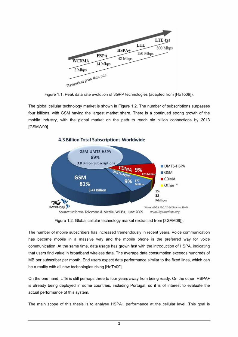
Figure 1.1. Peak data rate evolution of 3GPP technologies (adapted from [HoTo09]).
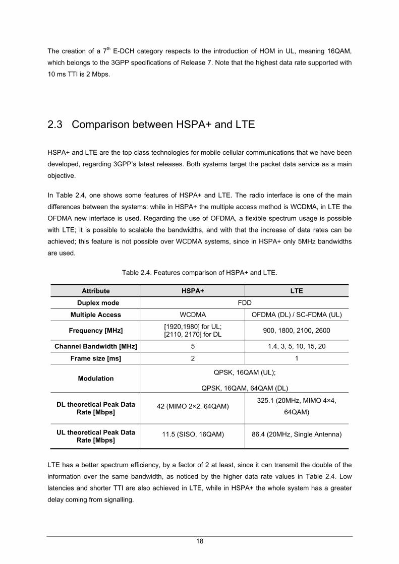
The global cellular technology market is shown in Figure 1.2. The number of subscriptions surpasses
four billions, with GSM having the largest market share. There is a continued strong growth of the
mobile industry, with the global market on the path to reach six billion connections by 2013
[GSMW09].
Figure 1.2. Global cellular technology market (extracted from [3GAM09]).
The number of mobile subscribers has increased tremendously in recent years. Voice communication
has become mobile in a massive way and the mobile phone is the preferred way for voice
communication. At the same time, data usage has grown fast with the introduction of HSPA, indicating
that users find value in broadband wireless data. The average data consumption exceeds hundreds of
MB per subscriber per month. End users expect data performance similar to the fixed lines, which can
be a reality with all new technologies rising [HoTo09].
On the one hand, LTE is still perhaps three to four years away from being ready. On the other, HSPA+
is already being deployed in some countries, including Portugal, so it is of interest to evaluate the
actual performance of this system.
The main scope of this thesis is to analyse HSPA+ performance at the cellular level. This goal is
3

4
accomplished by carrying out measurements in a single user scenario, studying the behaviour of
parameters such as throughput, Channel Quality Indicator (CQI) and modulation, using several
settings and under different radio channel conditions.
This thesis was made in collaboration with the Portuguese mobile telecommunications operator
Optimus. HSPA+ measurements were performed on Optimus’ network. Note that at the time of the
measurements HOM had already been introduced, unlike MIMO.
The main contribution of this thesis is the analysis of HSPA+ performance at the cellular level, in a
single user scenario, in both DL and UL. The comparison between measured and theoretical data is
also done.
This thesis is composed of 4 chapters, besides the current one, followed by a set of annexes.
In Chapter 2, an introduction to the main technologies that are related to the scope of this thesis is
presented, mainly focusing on the architecture, coverage and capacity aspects. First, a description of
HSPA and HSPA+ is provided. Later, a brief comparison between HSPA+ and LTE is shown. At the
end of the chapter, current services and applications are addressed.
Chapter 3 presents the theoretical models that are used in this work, as well as the parameters
required to compare expected and experimental data.
In Chapter 4, the measurements’ scenario is presented, describing the environment and the power
configurations. Afterwards, the HSPA+ DL and UL results are analysed, and the comparison with the
theoretical models is done.
Finally, in Chapter 5, the main conclusions of this work are drawn, along with future work suggestions.
A set of annexes with auxiliary information and additional results is also included. Annex A contains
the basic aspects of MIMO. In Annex B, one presents the detailed link budget. Finally, in Annex C, one
shows additional HSPA+ DL results.

Chapter 2
Basic Concepts 2 Basic Concepts
This chapter gives an introduction to the main technologies that are related to the scope of this thesis,
mainly focusing on the architecture, coverage and capacity aspects. First, a description of HSPA and
HSPA+ is provided. Later, a brief comparison between HSPA+ and LTE is presented. At the end of
the chapter, current services and applications are addressed.
5

2.1 UMTS/HSPA
In this section, based on [HoTo06], UMTS Releases 5 and 6 basic concepts are presented, namely
network architecture, radio interface and performance aspects.
2.1.1 Network Architecture
The UMTS architecture is represented in Figure 2.1, the network being grouped into three high-level
modules, which are specified by 3GPP:
• User Equipment (UE);
• UMTS Terrestrial Radio Access Network (UTRAN);
• Core Network (CN).
UE is, basically, the interface with the user, UTRAN deals with all radio related functionality, and
finally, CN handles switching and routing calls and data connection to external networks.
Figure 2.1. UMTS network architecture (extracted from [HoTo04]).
The UE is composed of the Mobile Equipment (ME) and the UMTS Subscriber Identity Module
(USIM). The ME is the Mobile Terminal (MT) used for radio communication over the Uu interface and
the USIM is a smart card that holds the subscriber identity, performs authentication algorithms and
stores information. USIM and ME communicate over the Cu interface.
UTRAN consists of one or more Radio Network Sub-Systems (RNSs), being composed of two
different elements:
• Node B, the Base Station (BS), switches the data flow between the Iub and Uu interfaces, with
some functionalities in the Radio Resource Management (RRM);
• Radio Network Controller (RNC) owns and controls the radio resources in Node Bs connected
to it by the Iub interface, carrying the major RRM functions, e.g., outer loop power control,
packet scheduling and handover control.
6

In UTRAN, RNCs are connected to each other by the Iur interface.
CN is adapted from GSM CN, the main elements being:
• Home Location Register (HLR) is a database located in the user’s home system;
• Mobile Switching Centre/Visitor Location Register (MSC/VLR) is the switch and the database
that serves the UE in its current location for Circuit-Switched (CS) services;
• Gateway MSC (GMSC) is the switch at the point where UMTS Public Land Mobile Network
(PLMN) is connected to external CS networks; it is where all incoming and outgoing CS
connections carry by;
• Serving GPRS Support Node (SGSN) that has similar functionalities to MSC/VLR, but is
normally used for Packet-Switched (PS) services;
• Gateway GPRS Support Node (GGSN) functionality is close to that of GMSC, but relative to
PS services.
2.1.2 Radio Interface
In the radio interface (identified as Uu in Figure 2.1), UMTS uses WCDMA, a wideband
Direct-Sequence Code Division Multiple Access (DS-CDMA) air interface. It has a chip rate of 3.84
Mcps, which leads to a channel bandwidth of 4.4 MHz, with a channel separation of 5 MHz. Currently,
UMTS uses only FDD, UMTS Terrestrial Radio Access (UTRA) occupying the band [1920, 1980] MHz
for UL and [2110, 2170] MHz for DL [Moli05].
WCDMA uses two types of codes for spreading and multiple access: channelisation and scrambling.
Channelisation codes, on spreading, are responsible for separating transmissions from the same
source, in DL at the same sector, and in UL are used to separate physical data and control information
from the same UE. These codes are Orthogonal Variable Spreading Factor (OVSF) ones, which allow
the Spreading Factor (SF) to be changed and orthogonality between codes to be maintained.
Therefore, the number of channelisation codes is given by SF. Scrambling codes are mainly used to
distinguish between cells and users. Scrambling is used on top of spreading so that the signal
bandwidth is not changed; in DL, it differentiates the sectors of the cell, and in UL it separates MTs
from each other, which allows the use of identical spreading codes for several transmitters.
HSDPA and HSUPA are Release 99 evolutions, both known as HSPA, and patented by 3GPP as
Release 5 and Release 6, respectively. While in Release 99 the scheduling control is based on the
RNC, and the Node B only has power control functionalities, in HSDPA capacity and spectral
efficiency are improved. Scheduling and fast link adaptation based on physical layer retransmissions
were moved to the Node B, reducing latency and providing a whole change in RRM.
In Release 99, radio transmissions are structured in frames of 10 ms, and transport data blocks are
transmitted over an integer number of frames. The Transmission Time Interval (TTI), which is the
transmission duration, is, usually, between 10 and 80 ms. HSPA supports a frame length of 2 ms,
7

which leads to the reduction of latency and a fast scheduling among different users.
HSDPA does not support soft handover or fast power control. Higher data rates are accomplished
through the use of 16 Quadrature Amplitude Modulation (QAM), which can only be used under good
radio channel conditions. Quaternary Phase Shift Keying (QPSK) is mainly used to maximise
coverage and robustness. HSDPA introduces Adaptive Modulation and Coding (AMC), which adjusts
the modulation and coding scheme to the radio channel conditions, and, together with 16QAM, allows
higher data rates.
Several new channels have been introduced for HSDPA operation. For user data, there are the High-
Speed Downlink Shared Channel (HS-DSCH) and the High-Speed Physical Downlink Shared Channel
(HS-PDSCH). For the associated signalling needs, there are two channels: High-Speed Shared
Control Channel (HS-SCCH) in the DL, and the High-Speed Dedicated Physical Control Channel (HS-
DPCCH) in the UL direction. For Release 6, the Fractional Dedicated Channel (F-DCH) was created
for handling power control when only packet services are active, allowing a larger number of users
with lower data rates [HoTo06].
The HS-DSCH supports the new 16QAM modulation. Node B scheduling with TTI of 2 ms and fast
physical layer transmission using Hybrid Automatic Repeat Request (HARQ) with two types of
retransmission are used. For user data transmission, HSDPA uses a fixed SF of 16, which means that
user data can be transmitted using up to 15 orthogonal codes, since the 16th is reserved for HS-
SCCH, allowing a theoretical peak bit rate of 14.4 Mbps. The HS-SCCH carries critical signalling
information for de-spreading of the correct codes and ARQ information providing the repetition of the
previous transmission based on received transmissions. It uses QPSK modulation and an SF of 128.
In order to keep a balanced evolution, there was the need to enhance UL as well. In Release 6,
HSUPA was introduced as an extension of Release 99, with the goal of achieving higher data rates
compared to Release 99’s 384 kbps in general urban outdoor scenarios, and later reaching 2 Mbps in
hot-spot, indoor areas.
HSUPA has some of the features of HSDPA, namely fast Layer-1 (L1) HARQ, fast Node B based
scheduling and, optionally, a shorter TTI of 2 ms, brought to UL with a new transport channel, the
Enhanced DCH (E-DCH). The HARQ used in HSUPA is fully synchronous, avoiding the need for
sequence numbering, and it can operate in soft handover. The modulation is Binary Phase Shift
Keying (BPSK), since transmission with multiple channels was adopted, instead of using higher order
modulation, avoiding severe changes on technical issues at the UE.
New operation channels were introduced. In UL, the E-DCH Dedicated Physical Control Channel
(E-DPCCH) is used for new control information, and for carrying data there is the E-DCH Dedicated
Physical Data Channel (E-DPDCH). In DL, the E-DCH Absolute Grant Channel (E-AGCH) and the
E-DCH Relative Grant Channel (E-RGCH) are used for scheduling control and the E-DCH HARQ
indicator channel (E-HICH) is used for retransmission support. The DCH channels from Release 99
8

were left unchanged. In HSUPA, the E-DCH is a dedicated channel, similar to Release 99, but with
fast retransmission and scheduling, while for HSDPA, the HS-DSCH is a shared one [HoTo06].
In HSDPA, one of the criteria for admission of new users is the available transmit power. On the other
hand, in HSUPA the common resource is the UL noise factor, directly connected to the interference
level, since each UE has its own transmitter. The scheduling main function is to keep the UL noise
factor low enough to allow a high cell capacity, assuring that cell overload is not reached.
Table 2.1 lists the applicability of key features for Release 99, HSDPA and HSUPA.
Table 2.1. Comparison between UMTS stages (adapted from [HoTo06]).
Feature Release 99 Release 5 (HSDPA) Release 6 (HSUPA)
Variable Spreading Factor Yes No Yes
Adaptive Modulation No Yes No
Soft Handover Yes No Yes
Fast Power Control Yes No Yes
Node B based scheduling No Yes Yes
Fast L1 HARQ No Yes Yes
TTI length [ms] 80, 40, 20, 10 2 10, 2
Maximum data rate [Mbps] 0.384 (urban outdoor) / 2 (indoor) 14.4 5.7
2.1.3 Coverage and Capacity
The trade-off between capacity and interference is of key importance in cellular networks. In UMTS,
capacity depends, essentially, on the number of users and on the type of services, via the interference
margin and the sharing of transmitting power. This margin is given by [Corr06]:
[ ] ( )η−−= 1log10dBIM (2.1)
where:
• η is the load factor.
A raise of the load factor leads to a reduction in coverage, via the increase of the interference margin.
The load factor depends on the services, and since there is asymmetry between UL and DL, it is
different between the two; it should not be higher than 50% in UL and 70% in DL. These factors, for a
given user j, are given by [Corr06]:
( )∑=
⋅ρ+
+=ηuN
j
jajN
jbcninterUL
F
RRI
1 1
11 (2.2)
9

10
( ) ( )[ jninterj
N
j jbc
jNjaninterDL I
RRFI
u
+α−ρ
+=η ∑=
1.11
] (2.3)
where:
• ηUL is the UL load factor;
• ηDL is the DL load factor;
• Iinter n is the normalised inter-cell interference (between [40, 60] % in UL and 0% in DL);
• Nu is the number of active users;
• Rc is the chip rate of WCDMA (3.84 Mcps);
• Rb j is the data rate associated to service of user j;
• ρN j is the Signal-to-Noise ratio (SNR) of user j;
• Fa j is the activity factor of user of user j (50% for voice and 100% for data);
• αj is the code orthogonality factor of user j (typically in [0.5, 0.9]).
The radius of a given cell can be estimated using the definition of the path loss and the model of the
average power decay with distance. The radius of a cell is given by [Corr06]:
[ ]
[ ] [ ] [ ] [ ] [ ]
pd
refrrtt
aLGPGP
R ⋅
−+−+
= 10km
dBdBidBmdBidBm
10 (2.4)
where:
• Pt is the power fed to the transmitting antenna;
• Gt is the gain of the transmitting antenna;
• Pr is the power available at the receiving antenna;
• Gr is the gain of the receiving antenna;
• Lref are propagation model losses;
• apd is the average power decay.
Release 99 uses Eb/N0, energy per bit to noise power spectral density ratio, as a metric to evaluate its
performance. In HSDPA, the bit rate can change every TTI using different modulation and coding
schemes. Therefore, the metric used for HSDPA is the average HS-DSCH Signal-to-Interference-plus-
Noise Ratio (SINR) that represents the narrowband SINR after the process of de-spreading of HS-
PDSCH. Link adaptation selects the modulation and coding schemes with the purpose of optimising
throughput and delay for the instantaneous SINR [HoTo06].
The HS-DSCH SINR for a single antenna Rake receiver is expressed by [HoTo06]:
( ) RFerintaintr
RxDSCHHS
IN NIIP
SF++⋅α−
=ρ −
116 (2.5)
where:

• ρIN is the SINR;
• SF16 is a HS-PDSCH spreading factor of 16;
• RxDSCHHSP − is the received power of the HS-DSCH summing over all active HS-PDSCH codes;
• Iintra is the received intra-cell interference;
• Iinter is the received inter-cell interference;
• NRF is the noise power at the radio frequency (RF) band.
HS-DSCH SINR is an important measure to network dimensioning and link budget planning. It is also
used to accomplish a certain Block Error Ratio (BLER) for the number of HS-PDSCH codes,
modulation and coding scheme used. Figure 2.2 illustrates the average throughput, including link
adaptation and HARQ, as a function of the average HS-DSCH SINR. Results are shown for 5, 10 and
15 HS-PDSCH codes.
Figure 2.2. HSDPA data rate as function of the average HS-DSCH SINR (extracted from [Pede05]).
The average cell throughput increases with the number of HS-PDSCH codes, having a growth of 50%
when the number of codes is modified from 5 to 10. HARQ, fast link adaptation and turbo-coding
contribute to have a capacity gain of almost 70% compared to Release 99 [HoTo06].
On the other hand, with the increase of the power allocated to HS-DSCH the data rates would be
higher as well, until it creates greater interference. For example, with 5 HS-PDSCH codes, 16QAM,
the HS-DSCH SINR should be in the range of [-3, 17] dB, [Salv08].
Network capacity depends on type of user and the respective scenario, type of service provided, and
number of HS-PDSCH codes used.
The Common Pilot Channel (CPICH) Ec/N0, pilot energy per chip to noise power spectral density ratio,
is frequently used to network dimensioning and to estimate single user throughput. SINR can be
11

expressed as a function of the pilot Ec/N0 [HoTo06]:
TxBS
pilot
Txpilot
TxDSCHHS
IN
PP
PSF
⋅α−ρ
=ρ −16 (2.6)
where:
• TxDSCHHSP − is the HS-DSCH transmit power;
• TxpilotP is the CPICH transmit power;
• ρpilot is the CPICH Ec/N0;
• TxBSP is the total Node B transmit power.
The HSDPA transmit power can be expressed as a function of the SINR, thus, as a function of the
desired data rate at the cell edge using:
16
1)1(SFP
gPTxBS
INTx
DSCHHS−
− +α−⋅ρ≥ (2.7)
where:
• g is the geometry factor, defined as:
RFerint
aintr
NII
g+
= (2.8)
As in HSDPA, performance in HSUPA depends highly on network algorithms, deployment scenarios,
UE transmitter capability, Node B performance and capability and type of traffic. For performance
testing purposes, 3GPP defined a set of E-DCH channel configurations called Fixed Reference
Channels (FRCs). FRC5 represents the first HSUPA phase UE, while FRC2 and FRC6 represent the
incoming UE’s releases with advanced capabilities, like higher coding rate and support 2 ms for TTI.
The performance metric used in HSUPA is Ec/N0. A high Ec/N0 at the Node B is necessary to achieve
higher data rates, leading to an increased UL noise and, as a result, a decreased cell coverage area.
For this reason, a maximum level for the UL noise may be defined for macro-cells, to guarantee the
coverage area, otherwise, limiting high data throughputs. In Figure 2.3, one presents the expected
data rate for vehicular UE as a function of the available E-DCH Ec/N0.
The relation between Eb/N0 and Ec/N0 is given by:
[dB][dB]0[dB]0 // Pcb GNENE += (2.9)
where:
• Gp is the processing gain, defined as:
12

⎟⎟⎠
⎞⎜⎜⎝
⎛=
b
cp R
RG log10[dB] (2.10)
Figure 2.3. HSUPA throughput in Vehicular A at 30 km/h, without power control (extracted from
[HoTo06]).
It is clear that the curves corresponding to FRC2 with 2 ms TTI and FRC6 with 10 ms TTI are similar.
Nevertheless, FRC2 can reach higher throughputs in circumstances of high enough Ec/N0 values,
which in real scenarios may be difficult to achieve. Values of received Ec/N0 higher than 0 dB allow, in
both cases, to obtain throughputs beyond 2 Mbps [HoTo06].
HSUPA, by using HARQ and a soft combination of HARQ retransmissions, allows a decrease of the
necessary Eb/N0 at the Node B, when comparing similar data rates with Release 99. Increasing the
Block Error Probability (BLEP) at first transmission increases the UL spectral efficiency and again
consequently a lower Eb/N0. The capacity improvement due to the use of HARQ is expected to be
between 15% and 20% [HoTo06].
Considering Node B based scheduling, it can provide the system two main advantages: faster
reallocation of radio resources among users, and tighter control of total received UL power. The
former dynamically takes resources from users with low utilisation of allocated radio resources and
redistributes them among users with high utilisation, while the latter allows faster adaptation to
interference variations. The use of HARQ and Node B scheduling improves a capacity gain of 15 to
60%, according to [Lope08], depending on the service and scenario.
There are 2 TTIs available: the 2 ms is used under good channel conditions and only for high data
rates, while the 10 ms is the default value for cell edge coverage suffering from a high number of
retransmissions due to the increased associated path loss [HoTo06].
13

2.2 HSPA+
In this section, HSPA+ main concepts are presented, based on [BEGG08] and [PWST07].
The aim of HSPA+ is to further improve UMTS performance, through higher peak data rates, greater
capacity, lower latency, and greater spectral efficiency. In order to support these enhanced
capabilities, HSPA+ introduces:
• HOM;
• MIMO;
• Continuous Packet Connectivity (CPC);
• Advanced Receivers;
• Layer-2 (L2) protocol enhancements;
• Multicast/Broadcast Single-Frequency Network (MBSFN);
• Enhanced Cell Forward Access Channel (CELL_FACH);
• Support optimisation for Voice over Internet Protocol (VoIP).
These new concepts will yield substantially higher peak data rates. In Release 8, for example, the
peak data rates will theoretically reach up to 42 Mbps in DL and 11.5 Mbps in UL (per 5 MHz carrier)
[BEGG08]. Additionally, for next specification releases, 3GPP is considering Downlink-Optimised
Broadcast (DOB) and multi-carrier operation.
HOM enables users to experience significantly higher data rates, under favourable radio conditions,
with the introduction in Release 6 of BPSK and QPSK in the UL and QPSK and 16QAM for the DL.
Furthermore, Release 7 incorporates 64QAM in DL, increasing the peak data rate to the double
[HoTo07] from 14.4 Mbps to around 28 Mbps in a 2x2 MIMO configuration.
MIMO increases the data rate by transmitting multiple transport blocks in parallel, using multiple
antennas, to a single user; taking advantage of spatial multiplexing, the receiver uses the channel,
modulation and coding schemes in order to separate the encoded streams. In Annex A, the basic
aspects of MIMO are presented.
The potential gain reachable with MIMO and HOM is illustrated in Figure 2.4 for the 90th percentile
throughput, for DL. The improvements verified for UL can be observed in Figure 2.5. Note the slightly
differences in DL with the use of multiple receiver branches SIMO, which extend the benefits of HOM
in lower SNRs, and the better power efficiency resulting in a better performance of QPSK compared
with 16QAM, when the data rate target is under 4 Mbps in the UL.
Moreover, in order to support the signalling of the new modulation schemes, larger transport block
sizes (TBS), HARQ per stream, and larger range for CQI, 3GPP updates several physical channels,
like HS-SCCH, HS-DPCCH, E-AGCH and E-DPCCH. Modulation and Coding Scheme (MCS) tables
determine the best combination of modulation and coding rate for a given SNR, leading to a limited
14

peak data rate, due to the use of the higher modulation and least amount of coding possible, for each
value of SNR.
Figure 2.4. The 90th percentile throughput for DL HOM and MIMO (extracted from [BEGG08]).
Figure 2.5. Throughput as a function of Ec/N0 for UL HOM (extracted from [PWST07]).
The receiver structures in UEs and Node Bs are constantly being improved to raise system
performance and increase user data bit rates. Release 6 and 7 introduced the use of receive diversity
antennas type-1, linear equalisers type-2, and the combination of linear equaliser with receive diversity
antennas. Release 8 introduces requirements for even more advanced receivers (type-3), with inter-
cell interference cancellation support.
15

With the activity level of packet users varying considerably over time, there is a need to efficiently
support continuously connected applications. The solution presented by 3GPP in Release 7 is CPC,
which has two main features called UE Discontinuous Transmission and Reception (UE DTX/DRX)
and HS-SCCH-less operation. The introduction of UE DTX/DRX leads to benefits, such as, reduced
battery consumption and increased capacity. In some situations of dense traffic transmission the
control channel HS-SCCH can carry a significant code overhead that is decreased by the “less
operation” referred above. In fact, this operation reduces code usage as well as interference from
control signalling and increases capacity. Simulations in [HGMT05] exhibit that the introduction of CPC
in Release 7 increases VoIP capacity by 40% in the UL and 10% in the DL.
The DL peak data rate is limited by the size of Radio Link Control (RLC) window, RLC Protocol Data
Unit (PDU) and by the RLC Round Trip Time (RTT). In order to support MIMO and 64QAM, a larger
RLC Protocol Data Unit is needed, therefore, in Release 7, flexible RLC PDU sizes are adopted as
well as Media Access Control (MAC) segmentation and MAC multiplexing for DL transmission. L2
protocol overhead is reduced, by reducing RLC header overhead, which is a consequence of the
ability of the transmitter to flexibly select the size of RLC PDUs. At the Node B level, a new protocol
was created, the MAC-ehs, which carries on the possibility of RLC PDUs segmentation, improving the
system coverage and reducing processing tasks at L2 [BEGG08].
The greater use of HSPA for Internet connections currently causes an impact on load and network
characteristics. Therefore, 3GPP has worked to enhance the CELL_FACH state in Release 7 and 8 in
order to keep up the data traffic level that has been carrying out. In Release 7, CELL_FACH has been
activated for the DL, whereas in Release 8, 3GPP improved the transport channel E-DCH in
CELL_FACH, enabling continuous data transmissions without interruptions even when channel
switching occurs. A critical enhancement in Release 7 that eliminates inter-cell interference is the use
of a common scrambling code on DL carriers for MBSFN transmission. The power efficiency is
improving beyond new levels, while now the limiting factor is associated with codes rather than power,
resulting in a larger ability of WCDMA technology concerning radio transmissions.
In Table 2.2, one presents the characteristics of MT categories for FDD HS-DSCH physical layer,
meaning HSDPA and HSPA+ DL. The inter-TTI parameter indicates the capability to sustain the peak
data rate over multiple continuous TTIs. Categories with a value of 1 correspond to devices that can
also sustain the peak rate during 2 ms over multiple TTIs, while terminals with an inter-TTI value
greater than 1 must wait for 2 or 4 ms after each received TTI [HoTo06].
Table 2.3 shows the HSUPA and HSPA+ UL MT categories’ characteristics.
3GPP standardised for HSDPA the common categories that go up to the 12th and the following ones
were frozen from Release 7 and 8, with the introduction of MIMO systems and in some cases dual cell
operation (21st to 24th MT categories).
16

Table 2.2. FDD HS-DSCH physical layer categories (adapted from [3GPP09a] and [HoTo07]).
MT Category
Maximum number of HS-PDSCH codes
received
Minimum inter-TTI
Supported Modulation
Supported Modulations with MIMO
Maximum theoretical peak data
rate [Mbps]
1
5
3
QPSK & 16QAM
Not applicable (MIMO
configurations not supported)
1.222 1.22 3
2 1.82
4 1.82 5
1
3.65 6 3.65 7
10 7.21
8 7.21 9
15 10.20
10 14.40 11
5 2
QPSK 0.91
12
1
1.82 13
15
QPSK, 16QAM & 64QAM
17.64 14 21.10 15
QPSK & 16QAM QPSK & 16QAM
23.37 16 27.95 17
QPSK, 16QAM & 64QAM
23.37 18 27.95 19 QPSK, 16QAM &
64QAM 35.28
20 42.20 21 --- --- 23.37 22 --- --- 27.95 23 --- --- 35.28 24 --- --- 42.20
Table 2.3. FDD E-DCH physical layer categories (adapted from [3GPP09a] and [HoTo06]).
MT Category
Maximum number of
E-DCH codes
transmitted
Minimum SF TTI length [ms]
Supported Modulation
Maximum theoretical
peak data rate [Mbps]
1 1 SF4 10
QPSK
0.71 2
2
2 x SF4 10, 2 1.45
3 10 1.45
4 2 x SF2
10, 2 2.89
5 10 2.00
6 4 2 x SF4 + 2 x SF2 10, 2
5.74
7 QPSK & 16QAM 11.50
17
The creation of a 7th E-DCH category respects to the introduction of HOM in UL, meaning 16QAM,
which belongs to the 3GPP specifications of Release 7. Note that the highest data rate supported with
10 ms TTI is 2 Mbps.
2.3 Comparison between HSPA+ and LTE
HSPA+ and LTE are the top class technologies for mobile cellular communications that we have been
developed, regarding 3GPP’s latest releases. Both systems target the packet data service as a main
objective.
In Table 2.4, one shows some features of HSPA+ and LTE. The radio interface is one of the main
differences between the systems: while in HSPA+ the multiple access method is WCDMA, in LTE the
OFDMA new interface is used. Regarding the use of OFDMA, a flexible spectrum usage is possible
with LTE; it is possible to scalable the bandwidths, and with that the increase of data rates can be
achieved; this feature is not possible over WCDMA systems, since in HSPA+ only 5MHz bandwidths
are used.
Table 2.4. Features comparison of HSPA+ and LTE.
Attribute HSPA+ LTE
Duplex mode FDD
Multiple Access WCDMA OFDMA (DL) / SC-FDMA (UL)
Frequency [MHz] [1920,1980] for UL; [2110, 2170] for DL 900, 1800, 2100, 2600
Channel Bandwidth [MHz] 5 1.4, 3, 5, 10, 15, 20
Frame size [ms] 2 1
Modulation QPSK, 16QAM (UL);
QPSK, 16QAM, 64QAM (DL)
DL theoretical Peak Data Rate [Mbps]
42 (MIMO 2×2, 64QAM) 325.1 (20MHz, MIMO 4×4,
64QAM)
UL theoretical Peak Data Rate [Mbps]
11.5 (SISO, 16QAM) 86.4 (20MHz, Single Antenna)
LTE has a better spectrum efficiency, by a factor of 2 at least, since it can transmit the double of the
information over the same bandwidth, as noticed by the higher data rate values in Table 2.4. Low
latencies and shorter TTI are also achieved in LTE, while in HSPA+ the whole system has a greater
delay coming from signalling.
18

In Table 2.5, one presents the comparison between UMTS and LTE network elements. In LTE, the
UMTS RNC functionalities are divided between evolved Node B (eNB), the single element of the
Evolved UTRAN (E-UTRAN), and Serving Gateway (S-GW), which has also the functionalities of
SGSN. The Packet Data Network (PDN) Gateway (P-GW) is similar to GGSN, while the Mobility
Management Entity (MME) has the functionalities of HLR and VLR in UMTS. MME, S-GW and P-GW
compose the Evolved Packet Core (EPC).
Table 2.5. Comparison between UMTS and LTE network elements.
Element UMTS LTE
Base Station Node B eNB
Controller RNC ---
Core Network / Evolved Packet Core
HLR - MSC/VLR MME
SGSN S-GW
GGSN P-GW
The LTE architecture is an IP-based flat one, with fewer elements and consequently simpler than the
hierarchical architecture used in HSPA+. On the other hand, HSPA+ is easier to implement, since
there is no need to modify the current network architecture, whereas in LTE there are several new
interfaces and functional upgrades.
2.4 Services and Applications
In order to manage the access to the different services and optimise system capacity, 3GPP defined
four classes of services based on their Quality of Service (QoS) requirements: Conversational,
Streaming, Interactive and Background. There are some important factors to distinguish them, such as
traffic delay, the guaranteed bit rate and the different priorities.
The Conversational class is mainly intended for speech services (e.g., CS or VoIP). Real time services
require tighter delay requirements to maintain a minimum quality of service. The delay order should
not overtake 400 ms [HoTo07], i.e., the maximum end-to-end delay given by the human perception for
audio and video conversation. Traffic is nearly symmetric between UL and DL. Video telephony has
even tighter Bit Error Ratio (BER) requirements than voice, due to video compression. When it works
on the PS domain, and in order to guarantee an efficient VoIP, service IP header compression and
QoS differentiation are needed. This class has priority over others, because voice is a primary service
and the one that is most required.
The Streaming class represents the audio and video streamings. This type of service enables the end
user to access the data before the transfer is complete, which is possible with the use of buffers in the
19

final applications and a continuous stream transmission. In this class, traffic is not symmetric, thus, DL
traffic is the most significant. Larger delays than in Conversational class can be tolerated, as the
receiver typically buffers several seconds of Streaming material.
The Interactive class has a very asymmetric traffic and is tolerant to delay. This class includes Web
browsing, online multiplayer games and push-to-talk applications, services that are based on PS
connections. These are characterised by requesting response patterns and preservation of payload
contents. Nevertheless, there are upper limits to tolerable delay, such as the time between choosing a
certain Website and its actual appearance on the screen, which should not exceed a few seconds. For
online multiplayer games, RTT is a very important parameter, especially in real time action games,
where the end-to-end delay should be below 100 ms [Lope08].
The Background class covers services where transmissions delays are not critical (e.g., Short
Messaging Service (SMS), Multimedia Messaging Service (MMS), E-mail), as opposed to the
Interactive one, where the end user is not waiting for a response within a short time; however, this
class is intolerant to transmission errors. Applications in this traffic class only use resource
transmissions when none of the other classes is active.
The main differences between the 3GPP classes are presented in Table 2.6.
Table 2.6. Services and applications according to 3GPP (extracted from [3GPP08]).
Service Class Conversational Streaming Interactive Background Real time Yes Yes No No
Symmetric Yes No No No Guaranteed bit rate Yes Yes No No
Delay Minimum Fixed Minimum Variable Moderate Variable High Variable Buffer No Yes Yes Yes Bursty No No Yes Yes
Switching Type CS CS PS PS Example Voice Video Streaming Web Browsing E-mail
20

21
Chapter 3
Models 3 Models
This chapter presents the theoretical models used throughout this work, as well as the parameters
needed to compare expected and experimental data.
3.1 HSPA+ DL
In this section, one presents the HSPA+ DL theoretical models of the several parameters under
analysis. For all the link budget aspects, refer to Annex B.
As mentioned in the previous chapter, the metric used in HSPA+ DL to evaluate the performance is
HS-DSCH SINR. Equations (2.5) and (2.6) give SINR as a function of HS-DSCH received power and
CPICH Ec/N0, respectively. It is also possible to relate SINR with the CPICH Received Signal Code
Power (RSCP), which is the received power on one code after de-spreading, measured on the
Primary CPICH [3GPP09b].
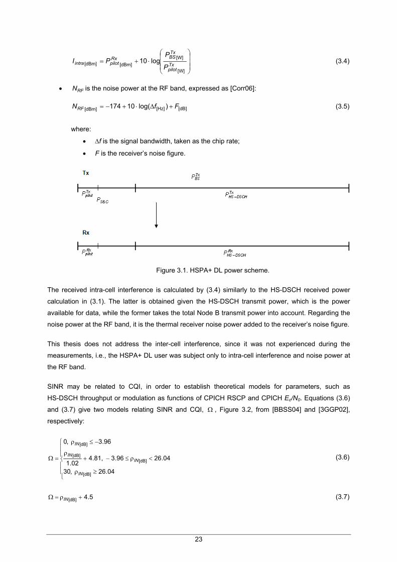
The HSPA+ DL power scheme is presented in Figure 3.1. Note that the propagation losses in the
CPICH and in the HS-DSCH are the same, so the HS-DSCH received power can be expressed as
[HoTo06]:
⎟⎟⎟
⎠
⎞
⎜⎜⎜
⎝
⎛⋅+=
−−
[W]
[W][dBm][dBm] log10
Txpilot
TxDSCHHSRx
pilotRx
DSCHHSP
PPP (3.1)
where:
• RxpilotP is the CPICH RSCP;
• TxDSCHHSP − is the HS-DSCH transmit power, given by:
][&][[W] WCSWTxBS
TxDSCHHS PPP −=− (3.2)
where:
• CSP & is the signalling and control power.
Manipulating (2.5) and (3.1), one has the SINR as a function of CPICH RSCP. Moreover, CPICH Ec/N0
can also be expressed as a function of CPICH RSCP [3GPP09b]:
⎟⎟⎟
⎠
⎞
⎜⎜⎜
⎝
⎛
++⋅=ρ
[W][W][W]
[W][dB]
log10RFerintaintr
Rxpilot
pilot NII
P (3.3)
where:
• aintrI is the received intra-cell interference, given by [HoTo06]:
22
23
⎟⎟⎟
⎠
⎞
⎜⎜⎜
⎝
⎛⋅+=
[W]
[W][dBm][dBm] log10
Txpilot
TxBSRx
pilotaintrP
PPI (
• N is the no
3.4)
ise power at the RF band, expressed as [Corr06]: RF
[dB][Hz][dBm] )log(10174 FfNRF +Δ⋅+−=
(3.5)
where:
Δf is the signal bandwidth, taken as the chip rate; •
• F is the receiver’s noise figure.
Figure 3.1. HSPA+ DL power scheme.
The received intra-cell interference is calculated by (3.4) similarly to the HS-DSCH received power
This thesis does not address the inter-cell interference, since it was not experienced during the
SINR may be related to CQI, in order to establish theoretical models for parameters, such as
calculation in (3.1). The latter is obtained given the HS-DSCH transmit power, which is the power
available for data, while the former takes the total Node B transmit power into account. Regarding the
noise power at the RF band, it is the thermal receiver noise power added to the receiver’s noise figure.
measurements, i.e., the HSPA+ DL user was subject only to intra-cell interference and noise power at
the RF band.
HS-DSCH throughput or modulation as functions of CPICH RSCP and CPICH Ec/N0. Equations (3.6)
and (3.7) give two models relating SINR and CQI, Ω , Figure 3.2, from [BBSS04] and [3GGP02],
respectively:
⎪⎪
⎩
⎪⎪
⎨
⎧
≥ρ
<ρ≤−+ρ
−≤ρ
=Ω
04.26,30
04.2696.3.81,402.1
96.3,0
[dB]
[dB][dB]
[dB]
IN
ININ
IN
(3.6)
(3.7) 5.4[dB] +ρ=Ω IN

24
Figure 3.2 shows that both
BLER is considered to be less than or equal to 10%.
models are similar and it was decided to use the one in (3.6). Note that the
0
5
10
15
20
25
30
-5 0 5 10 15 20 25 30
CQ
I
HS-DSCH SINR [dB]
[BBSS04] [3GPP02]
Figure 3.2. CQI as a function of HS-DSCH SINR.
For CQI definition, the UE a single HS-DSCH sub-
frame formatted with the TBS, number of HS-PDSCH codes and modulation corresponding to the
fined as the ratio of the number of erroneous blocks received to the total number of blocks
sent. An erroneous block is defined as a transport block, the cyclic redundancy check (CRC) of which
reports the highest tabulated CQI value for which
reported or lower CQI value could be received with a BLER not exceeding 10% [3GPP09c]. The CQI
mapping tables for MT categories 8 and 14 are presented in Table 3.1 and Table 3.2, respectively.
These tables define the TBS, number of codes and modulation that the MT should use for each CQI
and are used as a theoretical model throughout this thesis. The HS-DSCH throughput using these
UEs is approximated by dividing the TBS by TTI length (2 ms) and considering 16.7% for the
necessary overheads – 6.7% due to the RLC and MAC layers and 10% for BLER and application
[Lope08].
BLER is de
is wrong [3GPP09d]. HS-DSCH BLER can analytically be well approximated by [BBSS04]:
7.01
26.503.12 [dB]
−
⎟⎞
⎜⎛ +Ω⋅−ρ ⎤⎡ IN
)log(3 110⎟⎠
⎜⎝ Ω−
⎥⎥⎥
⎦⎢⎢⎢
⎣
+=ηBLER (3.8)
where:
• is the HS-DSCH BLER.
3.3 as a function of SINR for six different values of CQI,
from 5 to 30. One can observe a trend to a decrease of BLER with the increase of SINR for all CQI
BLERη
BLER on the HS-DSCH is illustrated in Figure
values. Note that the higher the SINR the greater the obtained CQI, given (3.6). Consequently, the
SINR needed to achieve BLER less than 10% increases when one considers higher CQIs.

25
Table 3.1. CQI mapping table for MT category 8 (adapted from [3GPP09c]).
CQI value Transport Block Size
[bits]
Number of HS-PDSCH
Codes Modulation
1 137
1
QPSK
2 173
3 233
4 317
5 377
6 461
7 650
2 8 792
9 931
1 1
3
0 262
1 11 483
12 1742
13 2279 4
14 2583
15 3319
5
16 3565
16QAM
17 4189
18 4664
19 5287
20 5887
21 6554
22 7168
23 9719 7
24 1 8 1418
25 1
10
4411
26 14411
27 14411
28 14411
29 14411
30 14411

Table 3.2. CQI mapping table for MT category 14 (adapted from [3GPP09c]).
CQI value Transport Block Size
[bits]
Number of HS-PDSCH
Codes Modulation
1 136
1
QPSK
2 176
3 232
4 320
5 376
6 464
7 648
2 8 792
9 928
10 1264
3 11 1488
12 1744
13 2288 4
14 2592
15 3328
5
16 3576
16QAM
17 4200
18 4672
19 5296
20 5896
21 6568
22 7184
23 9736 7
24 11432 8
25 14424 10
26 15776
64QAM 27 21768 12
28 26504 13
29 32264 14
30 38576 15
26

1
10
100
-5 0 5 10 15 20 25 30
HS-
DSC
H BL
ER
[%]
HS-DSCH SINR [dB]
5 10 15 20 25 30CQI
Figure 3.3. BLER as a function of SINR on HS-DSCH, considering different CQI values.
3.2 HSPA+ UL
As stated earlier, the performance metric used in HSPA+ UL is E-DCH Ec/N0. Physical throughput as a
function of Ec/N0 is given by (3.9) and (3.10), considering TTIs of 10 and 2 ms, respectively, and the
usage of QPSK [Preg08]. E-DCH throughput is obtained considering MAC and RLC overheads of
5.1% and BLER and application overhead equal to 10% [Lope08].
⎪⎪⎪
⎩
⎪⎪⎪
⎨
⎧
>
≤<−+⋅+⋅−⋅−
−≤<−+⋅+⋅
−≤≤−+⋅+⋅
=
1,2
15,9094.1)(0841.0)(0431.0)(0048.0
510,7137.1)(141.0)(0021.0
1013,02.9)(405.1)(055.0
[dB]0
[dB]0[dB]02
[dB]03
[dB]0
[dB]0[dB]02
[dB]0
[dB]0[dB]02
[dB]0
[Mbps]
NE
NENENENE
NENENE
NENENE
R
c
cccc
ccc
ccc
b
(3.9)
⎪⎪⎪
⎩
⎪⎪⎪
⎨
⎧
≤≤
<≤+⋅+⋅−⋅
<≤−+⋅+⋅−
−<≤−+⋅+⋅
=
116,7.5
62,04.1)(5012.2)(5429.0)(0417.0
21,77.3)(31.0)(05.0
110,8283.3)(5778.0)(0231.0
[dB]0
[dB]0[dB]02
[dB]03
[dB]0
[dB]0[dB]02
[dB]0
[dB]0[dB]02
[dB]0
[Mbps]
NE
NENENENE
NENENE
NENENE
R
c
cccc
ccc
ccc
b
(3.10)
In order to obtain E-DCH throughput as a function of CPICH RSCP, it is necessary to relate the latter
with E-DCH Ec/N0. Equation (B.10) gives Ec/N0 considering the received power in the Node B and total
noise power. The Node B received power can be related with RSCP, since the path loss is
approximately the same in UL and DL. Nevertheless, one should take the Node B diversity gain and
masthead amplifier gain into account, (3.11).
27

[dB][dB][W]
[W][dBm][dBm] log10 MHAdivTx
pilot
TxMTRx
pilotRx
BS GGP
PPP ++
⎟⎟⎟
⎠
⎞
⎜⎜⎜
⎝
⎛⋅+= (3.11)
where:
• RxBSP is the Node B received power;
• TxMTP is the MT transmit power;
• Gdiv is the diversity gain;
• GMHA is the masthead amplifier gain.
3.3 Assessment
Given the amount of data collected in measurements, parameters such as average and standard
deviation are used throughout this thesis, (3.12) and (3.13), respectively.
s
N
ii
N
zz
s
∑== 1
(3.12)
where:
• zi is the sample i;
• Ns is the number of samples.
∑=
−=σsN
ii
szz
N 1
2)(1
(3.13)
In order to compare experimental and expected results, one uses the relative mean error and Root
Mean Square Error (RMSE), (3.14) and (3.15), respectively. As reference value for the relative mean
error, the theoretical value is considered.
r
ir
zzz
e−
= (3.14)
where:
• zr is the reference value.
∑=
−=sN
iir
sRMS zz
Ne
1
2)(1
(3.15)
28

The correlation factor between two variables x and y is given by:
2
1
2
1
2
12
)()(
)()(
⎥⎥⎥⎥⎥⎥
⎦
⎤
⎢⎢⎢⎢⎢⎢
⎣
⎡
−⋅−
−⋅−
=
∑∑
∑
==
=
ss
s
N
ii
N
ii
N
iii
yyxx
yyxxr
(3.16)
29

30

31
Chapter 4
Results Analysis 4 Results Analysis
This chapter presents the results of the HSPA+ measurements that were performed. A description of
scenario and configurations is provided followed by the comparison between the collected data and
the theoretical models in both DL and UL.

4.1 Measurements Scenario
In this work, there was the possibility of carrying out HSPA+ measurements in a single user scenario,
in an Optimus site, using TEMS data collection software [Asco09]. Despite the fact that the MT was
inside a car, the environment may be considered indoor, given that the car was always parked during
the measurements and, therefore, mobility should not be taken into account. Since there are no
retransmissions in User Datagram Protocol (UDP), this transport layer protocol was chosen for the
measurements. A PERL script was used to force the continuous transfer of several files for 10
minutes.
The user was in ten locations within the cell radius to obtain results with average CPICH RSCP
varying between -110 and -65 dBm, corresponding to distance from Node B to MT between 0.22 and
0.65 km, Figure 4.1. In each location, six measurements were performed in DL and two in UL,
resulting in a total of eighty. In DL, one used a category 14 MT and an emulated category 8 MT by
imposing the usage of a maximum number of 10 HS-PDSCH codes and modulations QPSK and
16QAM. Both MTs had linear equaliser type-2 receivers. Concerning UL, an MT category 6 was used
to measure the performance with both 10 and 2 ms TTIs. Note that at the time of measurements HOM
had already been introduced, unlike MIMO.
Figure 4.1. Node B and measurements’ locations view (extracted from [GoEa09]).
In Table 4.1, one presents the total Node B transmit power, signalling and control power and data
power values of the HSPA+ DL measurements configurations, the latter calculated by (3.2). In Table
4.2, one shows the power values and activity factors of common channels for signalling and control,
which were CPICH, Broadcast Channel (BCH), Primary-Synchronisation Channel (P-SCH),
32

Secondary-Synchronisation Channel (S-SCH), HS-SCCH and an A-DCH for the signalling radio
bearer [Opti09].
Table 4.1. Power configurations of the HSPA+ DL measurements.
Power [dBm] TxBSP 45 43 41
CSP & 32.6
TxDSCHHSP − 44.7 42.6 40.3
Table 4.2. Power values and activity factors of common channels for signalling and control.
Channel Power [dBm] Activity Factor [%]
CPICH 29 100
BCH 25.9 90
P-SCH 27.2 10
S-SCH 25.5 10
HS-SCCH 27 100
A-DCH 19 100
The activity factors in Table 4.2 refer to typical values, the one relative to HS-SCCH being traffic
dependent [Opti09].
The receiver’s noise figure was 6 and 2.5 dB, considering MT and Node B, respectively. In UL, there
was no masthead amplifier gain, while the diversity gain was 2 dB.
4.2 HSPA+ DL
In this section, the comparison between the HSPA+ DL measurements results and the theoretical
models described in Chapter 3 is presented. The addressed parameters are HS-DSCH throughput,
CPICH Ec/N0, CQI, modulation ratio, number of used HS-PDSCH codes and HS-DSCH BLER.
Additional results are shown in Annex C.
4.2.1 HS-DSCH Throughput
The theoretical and experimental HS-DSCH throughputs as a function of CPICH RSCP considering
total Node B transmit power of 45 dBm are shown in Figure 4.2. In Figure 4.3 and Figure 4.4, one
33

34
presents additional results considering of 43 and 41 dBm, respectively. TxBSP
0
2
4
6
8
10
12
14
-110 -105 -100 -95 -90 -85 -80 -75 -70 -65
HS-
DSC
H Th
roug
hput
[M
bps]
CPICH RSCP [dBm]
10 Codes Theoretical 10 Codes Measured15 Codes Theoretical 15 Codes Measured
Figure 4.2. Theoretical and measured HS-DSCH throughputs as a function of CPICH RSCP using
both MTs, with .dBm45=TxBSP
Series “10 Codes” and “15 Codes” refer to the category 8 and 14 MT, respectively, corresponding to
the maximum number of HS-PDSCH codes used by each terminal. Since the experimental data
correspond to average values measured in each of the ten locations, standard deviations are also
shown. In Table 4.3, one shows the relative mean error and standard deviation between theoretical
and measured curves for the category 14 MT in Figure 4.2. It was necessary to choose the α in (2.5),
in order to minimise the relative mean error. Note that the orthogonality factor is not constant during
the measurements, depending on the distance from Node B to MT, therefore the relative mean errors
are high, the lowest being 36.9% for α equal to 0.9, with a standard deviation of 22.3%. It is also
important to mention that for high α values, the error decreases when CPICH RSCP increases, while
for low values of α the opposite happens. Regarding the category 8 MT, the value of α that minimises
the error is also 0.9, with relative mean error and standard deviation of 35.3% and 24.3%,
respectively. In this case, since the MT category was emulated, the performance was better than
expected for an actual category 8 MT. It should be reminded that the receiver was an equaliser type-2,
which allows greater DL orthogonality factor and, as a result, less intra-cell interference.
Table 4.3. Relative mean error and standard deviation of HS-DSCH throughput as a function of
CPICH RSCP for the category 14 MT, with depending on the α. dBm,45=TxBSP
α 0.1 0.2 0.3 0.4 0.5 0.6 0.7 0.8 0.9
e [%] 304 244 244 209 175 149 128 72.8 36.9 σ [%] 215 183 183 164 142 125 107 50.7 22.3
In Figure 4.2, one shows that for CPICH RSCP between -105 and -95 dBm, i.e., under unfavourable
radio channel conditions, the measured HS-DSCH throughput was similar for both MT categories,
being in the [2, 4] Mbps range, while as RSCP increased the difference between the data rates

increased as well, given the fact that 64QAM is used with high RSCP. The highest achieved data rate
was 8.26 and 10.9 Mbps, with mean CPICH RSCP of -74.1 and -74.3 dBm, using 10 and 15 HS-
PDSCH codes, respectively. It should be mentioned that the theoretical HS-DSCH throughput reaches
its maximum value for CPICH RSCP greater than -60 dBm for both MT categories, being constant for
RSCP between -94 and -60 dBm, which denotes that the used models are pessimistic.
02468
101214
-110 -105 -100 -95 -90 -85 -80 -75 -70 -65
HS-D
SCH
Thr
ough
put
[Mbp
s]
CPICH RSCP [dBm]
10 Codes Theoretical 10 Codes Measured15 Codes Theoretical 15 Codes Measured
Figure 4.3. Theoretical and measured HS-DSCH throughputs as a function of CPICH RSCP for both
MTs, with .dBm43=TxBSP
02468
101214
-110 -105 -100 -95 -90 -85 -80 -75 -70 -65 -60
HS-D
SCH
Thr
ough
put
[Mbp
s]
CPICH RSCP [dBm]
10 Codes Theoretical 10 Codes Measured15 Codes Theoretical 15 Codes Measured
Figure 4.4. Theoretical and measured HS-DSCH throughputs as a function of CPICH RSCP for both
MTs, with .dBm41=TxBSP
Figure 4.3 and Figure 4.4 exhibit the same trend of Figure 4.2; when there was an increase of RSCP,
the average measured throughput increased as well. Once more, the difference between data rates
was greater for RSCP higher than -85 dBm, i.e., only under good radio channel conditions the
category 14 MT can reach its maximum performance. With of 43 dBm the highest average
throughput was 7.9 and 11.6 Mbps, with mean RSCP of -74.4 and -74.2 dBm, using 10 and 15
HS-PDSCH codes, respectively, while considering equal to 41 dBm the average data rate
reached 8.23 and 12.6 Mbps, with mean RSCP equal to -63.4 and -70.5 dBm, for category 8 and 14,
TxBSP
TxBSP
35
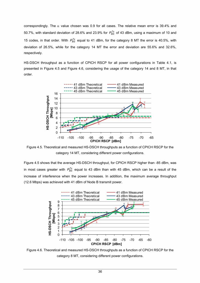
36
correspondingly. The α value chosen was 0.9 for all cases. The relative mean error is 39.4% and
50.7%, with standard deviation of 28.6% and 23.9% for of 43 dBm, using a maximum of 10 and
15 codes, in that order. With equal to 41 dBm, for the category 8 MT the error is 40.5%, with
deviation of 26.5%, while for the category 14 MT the error and deviation are 55.6% and 32.6%,
respectively.
TxBSP
TxBSP
HS-DSCH throughput as a function of CPICH RSCP for all power configurations in Table 4.1, is
presented in Figure 4.5 and Figure 4.6, considering the usage of the category 14 and 8 MT, in that
order.
02468
10121416
-110 -100 -95 -90 -85 -80 -75 -70 -65
HS-D
SCH
Thro
ughp
ut
[Mbp
s]
CPICH RSCP [dBm]-105
41 dBm Theoretical 41 dBm Measured43 dBm Theoretical 43 dBm Measured45 dBm Theoretical 45 dBm Measured
Figure 4.5. Theoretical and measured HS-DSCH throughputs as a function of CPICH RSCP for the
category 14 MT, considering different power configurations.
Figure 4.5 shows that the average HS-DSCH throughput, for CPICH RSCP higher than -85 dBm, was
in most cases greater with equal to 43 dBm than with 45 dBm, which can be a result of the
increase of interference when the power increases. In addition, the maximum average throughput
(12.6 Mbps) was achieved with 41 dBm of Node B transmit power.
TxBSP
0123456789
-110 -105 -100 -95 -90 -85 -80 -75 -70 -65 -60
HS-
DSC
H Th
roug
hput
[M
bps]
CPICH RSCP [dBm]
41 dBm Theoretical 41 dBm Measured43 dBm Theoretical 43 dBm Measured45 dBm Theoretical 45 dBm Measured
Figure 4.6. Theoretical and measured HS-DSCH throughputs as a function of CPICH RSCP for the
category 8 MT, considering different power configurations.
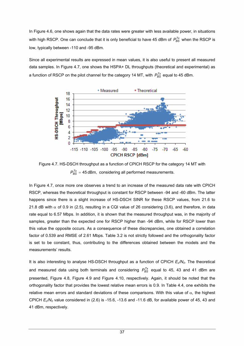
In Figure 4.6, one shows again that the data rates were greater with less available power, in situations
with high RSCP. One can conclude that it is only beneficial to have 45 dBm of when the RSCP is
low, typically between -110 and -95 dBm.
TxBSP
Since all experimental results are expressed in mean values, it is also useful to present all measured
data samples. In Figure 4.7, one shows the HSPA+ DL throughputs (theoretical and experimental) as
a function of RSCP on the pilot channel for the category 14 MT, with equal to 45 dBm. TxBSP
Figure 4.7. HS-DSCH throughput as a function of CPICH RSCP for the category 14 MT with
considering all performed measurements. dBm,45=TxBSP
In Figure 4.7, once more one observes a trend to an increase of the measured data rate with CPICH
RSCP, whereas the theoretical throughput is constant for RSCP between -94 and -60 dBm. The latter
happens since there is a slight increase of HS-DSCH SINR for these RSCP values, from 21.6 to
21.8 dB with α of 0.9 in (2.5), resulting in a CQI value of 26 considering (3.6), and therefore, in data
rate equal to 6.57 Mbps. In addition, it is shown that the measured throughput was, in the majority of
samples, greater than the expected one for RSCP higher than -94 dBm, while for RSCP lower than
this value the opposite occurs. As a consequence of these discrepancies, one obtained a correlation
factor of 0.539 and RMSE of 2.61 Mbps. Table 3.2 is not strictly followed and the orthogonality factor
is set to be constant, thus, contributing to the differences obtained between the models and the
measurements’ results.
It is also interesting to analyse HS-DSCH throughput as a function of CPICH Ec/N0. The theoretical
and measured data using both terminals and considering equal to 45, 43 and 41 dBm are
presented,
TxBSP
Figure 4.8, Figure 4.9 and Figure 4.10, respectively. Again, it should be noted that the
orthogonality factor that provides the lowest relative mean errors is 0.9. In Table 4.4, one exhibits the
relative mean errors and standard deviations of these comparisons. With this value of α, the highest
CPICH Ec/N0 value considered in (2.6) is -15.6, -13.6 and -11.6 dB, for available power of 45, 43 and
41 dBm, respectively.
37

Table 4.4. Relative mean error and standard deviation of HS-DSCH throughput as a function of
CPICH Ec/N0 with α = 0.9, considering different configurations.
TxBSP [dBm] 45 43 41
MT Category 8 14 8 14 8 14
e [%] 17.6 26.9 27.1 51.9 40.5 38.8 σ [%] 14.4 23.3 46.2 53.8 26.5 39.9
02468
1012141618
-20 -18 -16 -14 -12
HS-D
SCH
Thr
ough
put
[Mbp
s]
CPICH Ec/N0 [dB]
10 Codes Theoretical 10 Codes Measured15 Codes Theoretical 15 Codes Measured
Figure 4.8. Theoretical and measured HS-DSCH throughputs as a function of CPICH Ec/N0 using both
MTs, with . dBm45=TxBSP
In Figure 4.8, a trend to an increase of data rate with CPICH Ec/N0 is visible. According to the model,
with an Ec/N0 lower than -16 dB, the throughput should be approximately the same for both MTs,
whereas the experimental data show greater average throughput using the category 14 MT, for all
Ec/N0 values. The highest mean throughput was achieved with average Ec/N0 equal to -12.3 and -15.8
dB, in the measurements with 10 and 15 HS-PDSCH codes, respectively.
02468
1012141618
-19 -17 -15 -13 -11
HS-D
SCH
Thro
ughp
ut
[Mbp
s]
CPICH Ec/N0 [dB]
10 Codes Theoretical 10 Codes Measured15 Codes Theoretical 15 Codes Measured
Figure 4.9. Theoretical and measured HS-DSCH throughputs as a function of CPICH Ec/N0 for both
MTs, with .dBm43=TxBSP
38
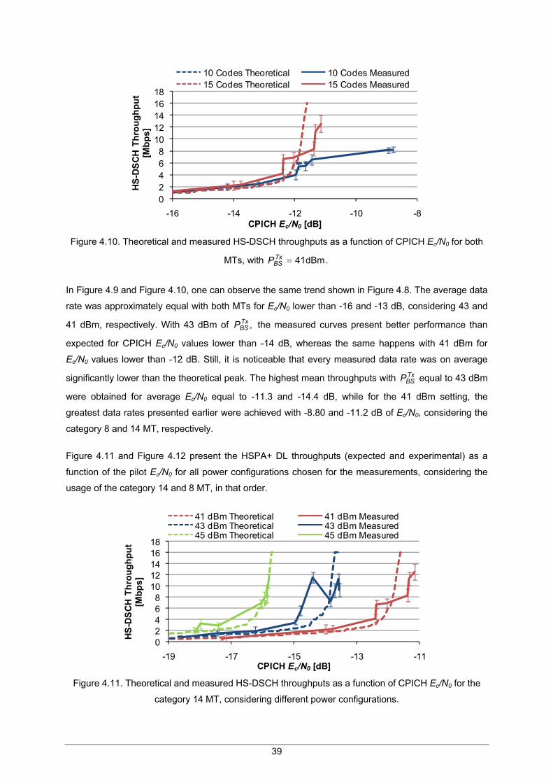
02468
1012141618
-16 -14 -12 -10 -8
HS-
DSC
H Th
roug
hput
[M
bps]
CPICH Ec/N0 [dB]
10 Codes Theoretical 10 Codes Measured15 Codes Theoretical 15 Codes Measured
Figure 4.10. Theoretical and measured HS-DSCH throughputs as a function of CPICH Ec/N0 for both
MTs, with .dBm41=TxBSP
In Figure 4.9 and Figure 4.10, one can observe the same trend shown in Figure 4.8. The average data
rate was approximately equal with both MTs for Ec/N0 lower than -16 and -13 dB, considering 43 and
41 dBm, respectively. With 43 dBm of the measured curves present better performance than
expected for CPICH Ec/N0 values lower than -14 dB, whereas the same happens with 41 dBm for
Ec/N0 values lower than -12 dB. Still, it is noticeable that every measured data rate was on average
significantly lower than the theoretical peak. The highest mean throughputs with equal to 43 dBm
were obtained for average Ec/N0 equal to -11.3 and -14.4 dB, while for the 41 dBm setting, the
greatest data rates presented earlier were achieved with -8.80 and -11.2 dB of Ec/N0, considering the
category 8 and 14 MT, respectively.
,TxBSP
TxBSP
Figure 4.11 and Figure 4.12 present the HSPA+ DL throughputs (expected and experimental) as a
function of the pilot Ec/N0 for all power configurations chosen for the measurements, considering the
usage of the category 14 and 8 MT, in that order.
02468
1012141618
-19 -17 -15 -13 -11
HS-D
SCH
Thr
ough
put
[Mbp
s]
CPICH Ec/N0 [dB]
41 dBm Theoretical 41 dBm Measured43 dBm Theoretical 43 dBm Measured45 dBm Theoretical 45 dBm Measured
Figure 4.11. Theoretical and measured HS-DSCH throughputs as a function of CPICH Ec/N0 for the
category 14 MT, considering different power configurations.
39

0
2
4
6
8
10
-20 -18 -16 -14 -12 -10 -8
HS-D
SCH
Thro
ughp
ut
[Mbp
s]
CPICH Ec/N0 [dB]
41 dBm Theoretical 41 dBm Measured43 dBm Theoretical 43 dBm Measured45 dBm Theoretical 45 dBm Measured
Figure 4.12. Theoretical and measured HS-DSCH throughputs as a function of CPICH Ec/N0 for the
category 8 MT, considering different power configurations.
Figure 4.11 and Figure 4.12 show that the model fits better for the setting with 45 dBm of , which
is reflected in the results of
TxBSP
Table 4.4. In Figure 4.11, the relative mean error is 26.9% for the
configuration with 45 dBm, being 51.9% and 38.8% with 43 and 41 dBm, respectively. Using the
category 8 MT, the errors are 17.6%, 27.1% and 40.5%, in the same order. It is visible that the higher
the available power, the lower the measured and theoretical CPICH Ec/N0. Subsection 4.2.2
addresses this parameter as a function of CPICH RSCP.
Taking all measured results into account, HS-DSCH throughputs (theoretical and experimental) as a
function of CPICH Ec/N0 for the category 14 MT with equal to 45 dBm are presented, TxBSP Figure 4.13.
Figure 4.13. HS-DSCH throughput as a function of CPICH Ec/N0 for the category 14 MT with
considering all performed measurements. dBm,45=TxBSP
As shown in Figure 4.13, measured Ec/N0 varied between -24 and -4.5 dB. The maximum theoretical
value of this parameter, for the chosen α of 0.9, is -15.6 dB, as stated earlier. This is a clear indication
that the orthogonality factor was not constant during the measurements. Note that the theoretical
model defines a trend to an increase of the throughput with CPICH Ec/N0 while the greatest measured
40
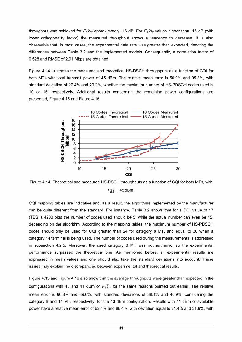
throughput was achieved for Ec/N0 approximately -16 dB. For Ec/N0 values higher than -15 dB (with
lower orthogonality factor) the measured throughput shows a tendency to decrease. It is also
observable that, in most cases, the experimental data rate was greater than expected, denoting the
differences between Table 3.2 and the implemented models. Consequently, a correlation factor of
0.528 and RMSE of 2.91 Mbps are obtained.
Figure 4.14 illustrates the measured and theoretical HS-DSCH throughputs as a function of CQI for
both MTs with total transmit power of 45 dBm. The relative mean error is 50.9% and 95.3%, with
standard deviation of 27.4% and 29.2%, whether the maximum number of HS-PDSCH codes used is
10 or 15, respectively. Additional results concerning the remaining power configurations are
presented, Figure 4.15 and Figure 4.16.
02468
1012141618
10 15 20 25 30
HS-
DSC
H Th
roug
hput
[M
bps]
CQI
10 Codes Theoretical 10 Codes Measured15 Codes Theoretical 15 Codes Measured
Figure 4.14. Theoretical and measured HS-DSCH throughputs as a function of CQI for both MTs, with
.dBm45=TxBSP
CQI mapping tables are indicative and, as a result, the algorithms implemented by the manufacturer
can be quite different from the standard. For instance, Table 3.2 shows that for a CQI value of 17
(TBS is 4200 bits) the number of codes used should be 5, while the actual number can even be 15,
depending on the algorithm. According to the mapping tables, the maximum number of HS-PDSCH
codes should only be used for CQI greater than 24 for category 8 MT, and equal to 30 when a
category 14 terminal is being used. The number of codes used during the measurements is addressed
in subsection 4.2.5. Moreover, the used category 8 MT was not authentic, so the experimental
performance surpassed the theoretical one. As mentioned before, all experimental results are
expressed in mean values and one should also take the standard deviations into account. These
issues may explain the discrepancies between experimental and theoretical results.
Figure 4.15 and Figure 4.16 also show that the average throughputs were greater than expected in the
configurations with 43 and 41 dBm of , for the same reasons pointed out earlier. The relative
mean error is 60.8% and 89.6%, with standard deviations of 38.1% and 40.9%, considering the
category 8 and 14 MT, respectively, for the 43 dBm configuration. Results with 41 dBm of available
power have a relative mean error of 62.4% and 86.4%, with deviation equal to 21.4% and 31.6%, with
TxBSP
41

42
maximum usage of 10 and 15 codes, respectively. These values represent the high divergence
between the models in Table 3.1 and Table 3.2 and the experimental data.
02468
1012141618
5 10 15 20 25 3
HS-D
SCH
Thro
ughp
ut
[Mbp
s]
CQI 0
10 Codes Theoretical 10 Codes Measured15 Codes Theoretical 15 Codes Measured
Figure 4.15. Theoretical and measured HS-DSCH throughputs as a function of CQI for both MTs, with
.dBm43=TxBSP
02468
1012141618
5 10 15 20 25
HS-
DSC
H Th
roug
hput
[M
bps]
CQI 30
10 Codes Theoretical 10 Codes Measured15 Codes Theoretical 15 Codes Measured
Figure 4.16. Theoretical and measured HS-DSCH throughputs as a function of CQI for both MTs, with
.dBm41=TxBSP
The HSPA+ DL throughput as a function of CQI considering all power configurations, for the category
14 device, is shown in Figure 4.17. Figure 4.18 presents the results using the category 8 MT. One can
see that the achieved throughput was similar for all power settings (being higher than the theoretical),
given the same CQI. This is expected since the model is independent of the available power.
In Figure 4.19, one shows the HS-DSCH throughputs (theoretical and experimental) as a function of
CQI for the category 14 MT, with equal to 45 dBm, taking all measured results into consideration.
One can observe a trend to an increase of the measured HS-DSCH throughput with CQI, as predicted
in the model, resulting in a correlation factor of 0.772. However, as expected from the analysis with
mean values, the measured throughput was, most of time, higher than the experimental one, the
RMSE being 2.91 Mbps. It is shown that the manufacturer did not take the CQI mapping tables into
account, which leads to the errors obtained in the comparisons that use
TxBSP
Table 3.1 and Table 3.2 as
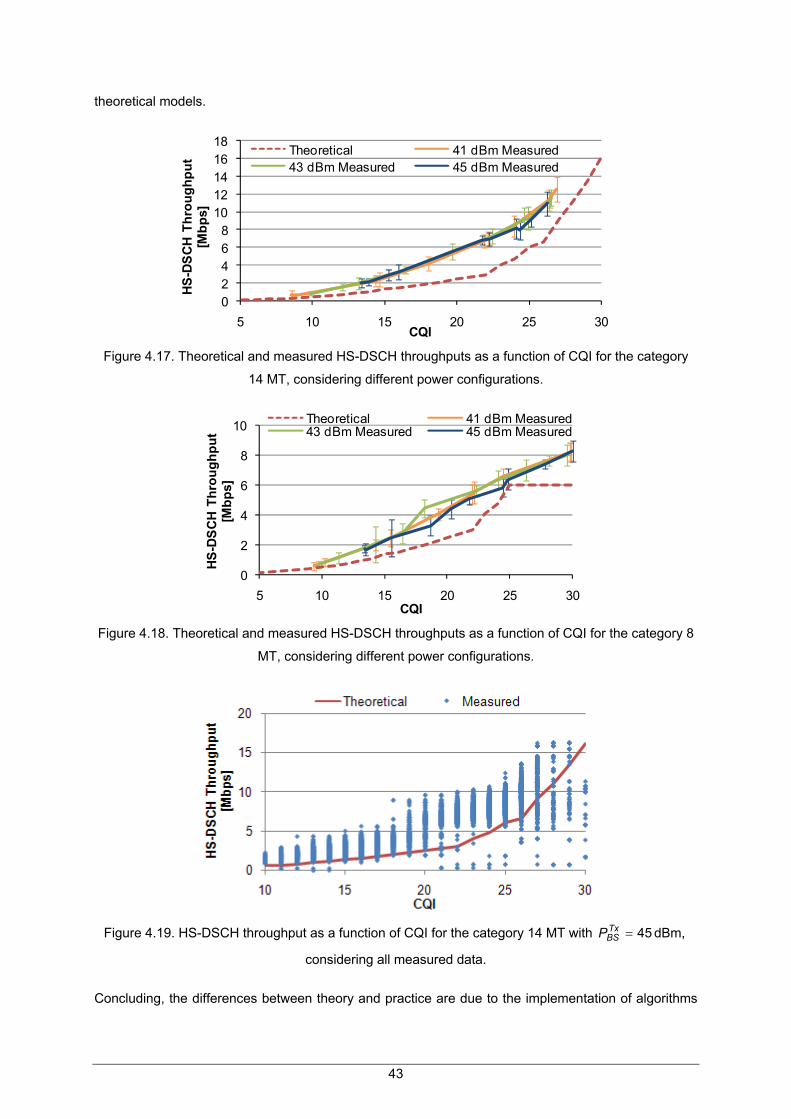
43
theoretical models.
02468
1012141618
5 10 15 20 25
HS-D
SCH
Thro
ughp
ut
[Mbp
s]
CQI 30
Theoretical 41 dBm Measured43 dBm Measured 45 dBm Measured
Figure 4.17. Theoretical and measured HS-DSCH throughputs as a function of CQI for the category
14 MT, considering different power configurations.
0
2
4
6
8
10
5 10 15 20 25 3
HS-D
SCH
Thro
ughp
ut
[Mbp
s]
CQI 0
Theoretical 41 dBm Measured43 dBm Measured 45 dBm Measured
Figure 4.18. Theoretical and measured HS-DSCH throughputs as a function of CQI for the category 8
MT, considering different power configurations.
Figure 4.19. HS-DSCH throughput as a function of CQI for the category 14 MT with
considering all measured data.
dBm,45=TxBSP
Concluding, the differences between theory and practice are due to the implementation of algorithms

that do not follow the CQI mapping tables, together with the use of an emulated 8th category MT and
the choice of fixed orthogonality factors. In addition, note that the maximum throughput measured was
16.3 and 12.6 Mbps with the category 14 MT, considering instantaneous and mean value,
respectively.
4.2.2 CPICH Ec/N0
Equation (3.3) gives CPICH Ec/N0 as a function of CPICH RSCP. The theoretical and experimental
data for this relation considering a maximum usage of 15 HS-PDSCH codes and all power
configurations are presented, Figure 4.20. In Figure 4.21, one shows the results for the category 8 MT.
-22-20-18-16-14-12-10
-120 -115 -110 -105 -100 -95 -90 -85 -80 -75 -70 -65 -60
CPIC
H E
c/N
0[d
B]
CPICH RSCP [dBm]
41 dBm Theoretical 41 dBm Measured43 dBm Theoretical 43 dBm Measured45 dBm Theoretical 45 dBm Measured
Figure 4.20. Theoretical and measured CPICH Ec/N0 as a function of CPICH RSCP for the category
14 MT, considering different power configurations.
In Figure 4.20, one shows that the greater the available power, the lower the achieved CPICH Ec/N0.
Still, with poor channel quality, e.g., for an RSCP of -105 dBm, the differences between the obtained
Ec/N0 values were smaller than for higher RSCP. The highest average Ec/N0 measured was -15.7,
-13.6 and -11.2 dB, considering equal to 45, 43 and 41 dBm, respectively. These results can be
explained with the trend to an increase of interference with power, which leads to a decrease of Ec/N0,
as the model forecasts. In theory, one should obtain the maximum CPICH Ec/N0 for an RSCP near
-100 dBm, whereas the experimental Ec/N0 saturated for RSCP between -90 and -80 dBm, resulting in
greater relative errors for low RSCP values.
TxBSP
In Figure 4.21, it is noticeable that the average CPICH Ec/N0 exceeded the theoretical maximum for
high RSCP. In fact, the greatest measured Ec/N0 was -12.3, -11.3 and -8.80 dB, considering
equal to 45, 43 and 41 dBm, respectively. Again, the differences between the measured Ec/N0 present
a trend to increase with RSCP.
TxBSP
Table 4.5 contains the relative mean error and standard deviation between the theoretical and the
measured data. Note that the configuration with the highest available power and 15 HS-PDSCH codes
usage has the lowest error, which is 6.13%. Moreover, all errors are lower than 20%, indicating a good
44
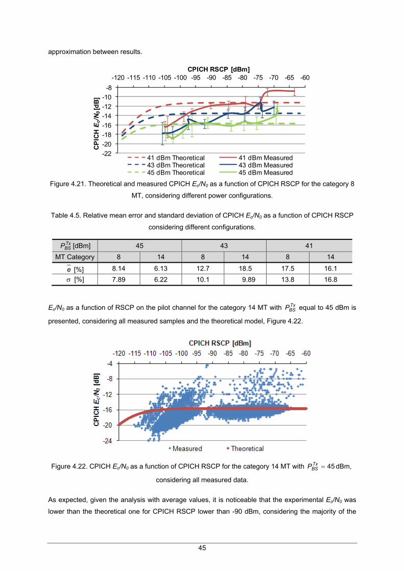
approximation between results.
-22-20-18-16-14-12-10
-8-120 -115 -110 -105 -100 -95 -90 -85 -80 -75 -70 -65 -60
CPI
CH E
c/N
0[d
B]
CPICH RSCP [dBm]
41 dBm Theoretical 41 dBm Measured43 dBm Theoretical 43 dBm Measured45 dBm Theoretical 45 dBm Measured
Figure 4.21. Theoretical and measured CPICH Ec/N0 as a function of CPICH RSCP for the category 8
MT, considering different power configurations.
Table 4.5. Relative mean error and standard deviation of CPICH Ec/N0 as a function of CPICH RSCP
considering different configurations.
TxBSP [dBm] 45 43 41
MT Category 8 14 8 14 8 14
e [%] 8.14 6.13 12.7 18.5 17.5 16.1 σ [%] 7.89 6.22 10.1 9.89 13.8 16.8
Ec/N0 as a function of RSCP on the pilot channel for the category 14 MT with equal to 45 dBm is
presented, considering all measured samples and the theoretical model,
TxBSP
Figure 4.22.
Figure 4.22. CPICH Ec/N0 as a function of CPICH RSCP for the category 14 MT with
considering all measured data.
dBm,45=TxBSP
As expected, given the analysis with average values, it is noticeable that the experimental Ec/N0 was
lower than the theoretical one for CPICH RSCP lower than -90 dBm, considering the majority of the
45

collected samples. In addition, Ec/N0 exceeded the theoretical maximum of -15.7 dB in several
occasions. As a result, one obtains an RMSE of 1.98 dB. The correlation factor is 0.544, since the
measured CPICH Ec/N0 did not always follow the theoretical trend.
It is also interesting to analyse how HSPA+ DL activity affected CPICH Ec/N0, i.e., what was,
considering the same RSCP, the degradation of Ec/N0 between situations without and with load. In
Figure 4.23, one presents this analysis using the category 14 MT with 45 dBm of available power.
-21
-17
-13
-9
-5
-1-105 -100 -95 -90 -85 -80 -75 -70
Ave
rage
CP
ICH
Ec/
N0
[dB]
Average CPICH RSCP [dBm]
Load No Load Figure 4.23. Measured CPICH Ec/N0 as a function of CPICH RSCP using the category 14 MT with
considering situations with and without HSPA+ DL activity. dBm,45=TxBSP
Results denote that the difference between Ec/N0 values increased as the path loss decreased, i.e.,
when there was an increase of the RSCP. In fact, while data were being transmitted the average
CPICH Ec/N0 saturated for RSCP around -88 dBm and did not exceed -15.8 dB. On the contrary, the
mean Ec/N0 without HSPA+ DL activity reached a maximum of -2.96 dB with an average RSCP equal
to -71.4 dBm. In summary, Ec/N0 degradation varied between 3.47 and 12.9 dB, with average value of
9.52 dB and standard deviation of 3.75 dB.
To sum up, one can conclude that the average measured Ec/N0 was close to expected, considering
the model in (3.3). Still, a correlation factor of 0.544 and RMSE of 1.98 dB are achieved, taking all
experimental values into account.
4.2.3 CQI
As mentioned earlier, CQI can be expressed as a function of CPICH Ec/N0 using (2.6) and (3.6). The
theoretical and measured data considering 45 dBm of total transmit power are shown for both
terminals, Figure 4.24. When the 15 HS-PDSCH codes were used, the highest CQI measured was 26,
with -15.8 dB of Ec/N0, while for 10 codes the maximum CQI was 30 when Ec/N0 reached -12.3 dB.
One can see a tendency to an increase of theoretical and measured CQIs with CPICH Ec/N0, given the
increase of HS-DSCH SINR.
46

47
10
15
20
25
30
-20 -18 -16 -14 -12
CQ
I
CPICH Ec/N0 [dB]
10 Codes Theoretical 10 Codes Measured15 Codes Theoretical 15 Codes Measured
Figure 4.24. Theoretical and measured CQIs as a function of CPICH Ec/N0 for both MTs, with
.dBm45=TxBSP
In Table 4.6, one shows the relative mean error and standard deviation between the theoretical and
measured curves for the category 14 MT in Figure 4.24, considering different values of orthogonality
factor. The lowest relative mean error is 8.92% with 5.84% of standard deviation, for α equal to 0.8.
Concerning the MT that uses a maximum of 10 HS-PDSCH codes, the α chosen was 0.6, resulting in
11.3% and 5.05% of relative mean error and standard deviation, respectively. As stated before, the
orthogonality factor depends on the distance, so when it is assumed a fixed α the errors are inevitable.
Nevertheless, the results show that the use of these theoretical models is appropriate.
Table 4.6. Relative mean error and standard deviation of CQI as a function of CPICH Ec/N0 for the
category 14 MT, with depending on the α. dBm,45=TxBSP
α 0.1 0.2 0.3 0.4 0.5 0.6 0.7 0.8 0.9
e [%] 31.9 26.7 26.4 22.8 18.6 16.5 11.9 8.92 11.2 σ [%] 24.6 20.2 18.2 15.2 11.9 8.81 6.72 5.84 6.45
In Figure 4.25 and Figure 4.26, one shows the results for both MTs, considering equal to 43 and
41 dBm, respectively.
TxBSP
In the measurements with the maximum usage of 10 HS-PDSCH codes the highest CQI was 30 for
Ec/N0 of -11.3 and -8.80 dB, with 43 and 41 dBm of respectively, while using 15 codes the
greatest CQI was 27 for -14.4 and -11.2 dB of Ec/N0, in the same order. The orthogonality factors
considered in
,TxBSP
Figure 4.25 and Figure 4.26 were 0.7 and 0.8, for the category 8 and 14 MT,
respectively. One can see that the experimental CQI followed the theoretical trend. With 43 dBm of
the relative mean error is 9.74% and 11.4%, with 8.37% and 9.08% of standard deviation, for the
category 8 and 14, correspondingly, while for 41 dBm the error is 9.06% and 10.1%, with deviation of
6.86% and 6.46%, in the same order. These results are representative of the minor discrepancies
between theoretical and measured data.
TxBSP
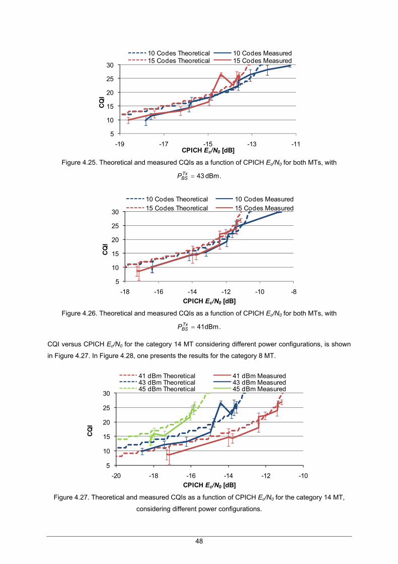
5
10
15
20
25
30
-19 -17 -15 -13 -11
CQ
I
CPICH Ec/N0 [dB]
10 Codes Theoretical 10 Codes Measured15 Codes Theoretical 15 Codes Measured
Figure 4.25. Theoretical and measured CQIs as a function of CPICH Ec/N0 for both MTs, with
.dBm43=TxBSP
5
10
15
20
25
30
-18 -16 -14 -12 -10 -8
CQ
I
CPICH Ec/N0 [dB]
10 Codes Theoretical 10 Codes Measured15 Codes Theoretical 15 Codes Measured
Figure 4.26. Theoretical and measured CQIs as a function of CPICH Ec/N0 for both MTs, with
.dBm41=TxBSP
CQI versus CPICH Ec/N0 for the category 14 MT considering different power configurations, is shown
in Figure 4.27. In Figure 4.28, one presents the results for the category 8 MT.
5
10
15
20
25
30
-20 -18 -16 -14 -12 -10
CQ
I
CPICH Ec/N0 [dB]
41 dBm Theoretical 41 dBm Measured43 dBm Theoretical 43 dBm Measured45 dBm Theoretical 45 dBm Measured
Figure 4.27. Theoretical and measured CQIs as a function of CPICH Ec/N0 for the category 14 MT,
considering different power configurations.
48

5
10
15
20
25
30
-20 -18 -16 -14 -12 -10 -8
CQI
CPICH Ec/N0 [dB]
41 dBm Theoretical 41 dBm Measured43 dBm Theoretical 43 dBm Measured45 dBm Theoretical 45 dBm Measured
Figure 4.28. Theoretical and measured CQIs as a function of CPICH Ec/N0 for the category 8 MT,
considering different power configurations.
Figure 4.27 and Figure 4.28 show that for a given CPICH Ec/N0, the higher the available power, the
greater the achieved CQI. As shown in the previous subsection, Ec/N0 increases with which
means that the CQIs were reached with higher Ec/N0 when lesser power was available.
,TxBSP
In Figure 4.29, one presents CQI as a function of CPICH Ec/N0, considering all experimental samples
and theoretical data, for the terminal of 14th category and 45 dBm of .TxBSP
Figure 4.29. CQI as a function of CPICH Ec/N0 for the category 14 MT with
considering all measured data.
dBm,45=TxBSP
Again, one observes a trend to an increase of CQI with CPICH Ec/N0, both in theory and in practice.
This is reflected in the correlation factor, which is 0.639. It is noticeable that, in the great majority of
cases, Ec/N0 did not exceed the maximum theoretical value (-15 dB), being the orthogonality factor
0.8. Still, results indicate that α was varying during the measurements. First, measured CQI presents a
significant variation for any given Ec/N0, resulting in an RMSE of 3. Additionally, CPICH Ec/N0 reached
values that are only specified with lower orthogonality factor values in (2.6).
49
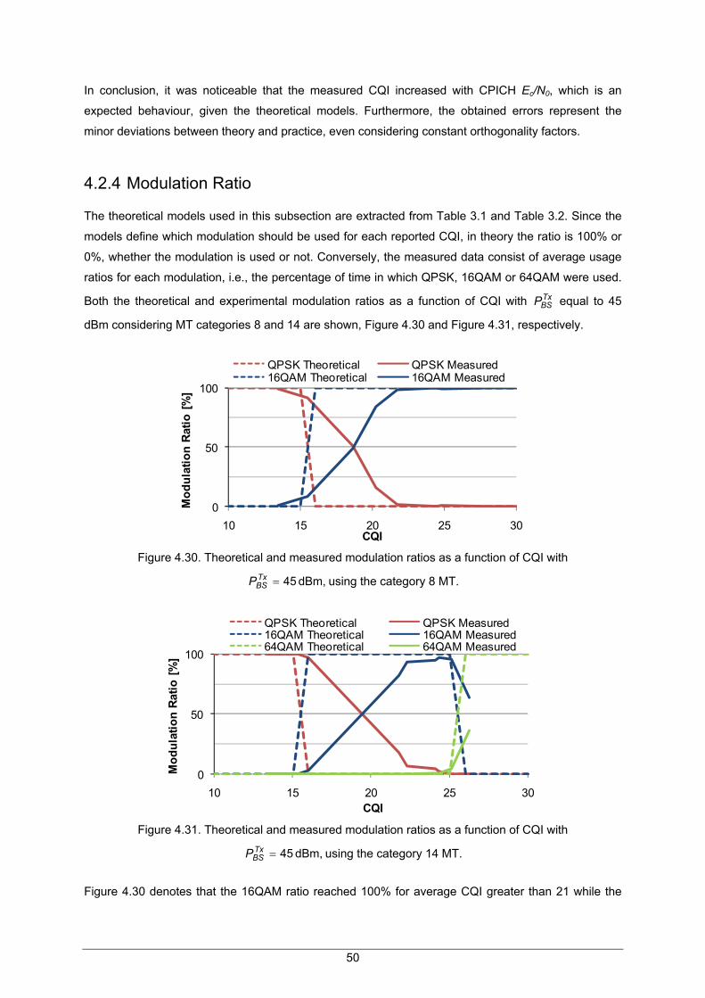
50
In conclusion, it was noticeable that the measured CQI increased with CPICH Ec/N0, which is an
expected behaviour, given the theoretical models. Furthermore, the obtained errors represent the
minor deviations between theory and practice, even considering constant orthogonality factors.
4.2.4 Modulation Ratio
The theoretical models used in this subsection are extracted from Table 3.1 and Table 3.2. Since the
models define which modulation should be used for each reported CQI, in theory the ratio is 100% or
0%, whether the modulation is used or not. Conversely, the measured data consist of average usage
ratios for each modulation, i.e., the percentage of time in which QPSK, 16QAM or 64QAM were used.
Both the theoretical and experimental modulation ratios as a function of CQI w TxBSP equal to 45
dBm considering MT categories 8 and 14 are shown,
ith
ely. Figure 4.30 and Figure 4.31, respectiv
0
50
100
10 15 20 25 30
Mod
ulat
ion
Rat
io [
%]
CQI
QPSK Theoretical QPSK Measured16QAM Theoretical 16QAM Measured
Figure 4.30. Theoretical and measured modulation ratios as a function of CQI with
using the category 8 MT. dBm,45=TxBSP
0
50
100
10 15 20 25 30
Mod
ulat
ion
Ratio
[%]
CQI
QPSK Theoretical QPSK Measured16QAM Theoretical 16QAM Measured64QAM Theoretical 64QAM Measured
Figure 4.31. Theoretical and measured modulation ratios as a function of CQI with
using the category 14 MT. dBm,45=TxBSP
Figure 4.30 denotes that the 16QAM ratio reached 100% for average CQI greater than 21 while the

model predicts its usage for CQI higher than 15. Nevertheless, since the comparison is done between
fixed and mean values, the model can be considered appropriate for this relation. One obtains 16.1%
of relative mean error with a standard deviation of 30.9%.
Regarding the 14th category MT, the relative error and standard deviation are 20% and 33.2%, in that
order. In Figure 4.31, one shows that the QPSK usage was greater than expected given the measured
CQI, leading to a lower 16QAM usage. Since the measured CQI did not achieve values greater than
26, there is not enough data to analyse the 64QAM ratio. Still, it should be noted that for an average
CQI of 26, the measured 64QAM ratio was 36.5%, distant from the theoretical 100%.
In Figure 4.32, one presents the comparison between the theoretical and measured modulation ratios
as a function of CPICH RSCP for the terminal of 8th category, with total transmit power equal to
45 dBm. Equivalent comparison concerning the MT that can use 64QAM is also shown, Figure 4.33.
0
50
100
-115 -110 -105 -100 -95 -90 -85 -80 -75 -70
Mod
ulat
ion
Ratio
[%]
CPICH RSCP [dBm]
QPSK Theoretical QPSK Measured16 QAM Theoretical 16QAM Measured
Figure 4.32. Theoretical and measured modulation ratios as a function of CPICH RSCP with
using the category 8 MT. dBm,45=TxBSP
The α value in (2.5) that gives the lowest relative mean error for both MTs is 0.1. Even taking the
lowest orthogonality factor into account, the model surpasses what was measured, which means that
the used model is very optimistic for this relation. For all measured CPICH RSCP average values
using the category 8 MT, the model indicates the usage of 16QAM for α between 0.1 and 0.9,
resulting in a relative mean error of 36% with standard deviation of 44.9%. As mentioned earlier, the
orthogonality factor depends on the distance and it varied during the measurements. Therefore, it is
supposed to be greater in situations with high received signal, normally when the MT is near the Node
B.
The relative mean error is minimised with 0.1 of orthogonality factor, being 47.2% with 45.8% of
standard deviation. Nevertheless, the 64QAM theoretical curve shown in Figure 4.33 was obtained for
α equal to 0.9, since that is the only value defining the usage of this modulation for RSCP lower than
-60 dBm, according to the models presented in the previous chapter. Once again, the achieved errors
for this relation are significant, which can be justified by the fact that the implemented algorithms differ
51

from the several models used, together with the use of mean experimental values in these analyses.
0
50
100
-115 -110 -105 -100 -95 -90 -85 -80 -75 -70
Mod
ulat
ion
Ratio
[%]
CPICH RSCP [dBm]
QPSK Theoretical QPSK Measured16QAM Theoretical 16QAM Measured64QAM Theoretical 64QAM Measured
Figure 4.33. Theoretical and measured modulation ratios as a function of CPICH RSCP with
using the category 14 MT. dBm,45=TxBSP
The relation between the modulation ratio and the CPICH Ec/N0 considering the MT that uses QPSK
and 16QAM, for a total transmit power of 45 dBm, is presented, Figure 4.34.
0
50
100
-20 -19 -18 -17 -16 -15 -14
Mod
ulat
ion
Rat
io [
%]
CPICH Ec/N0 [dB]
QPSK Theoretical QPSK Measured16QAM Theoretical 16QAM Measured
Figure 4.34. Theoretical and measured modulation ratios as a function of CPICH Ec/N0 with
using the category 8 MT. dBm,45=TxBSP
The smallest relative mean error between model and measured data is 7.8%, with standard deviation
equal to 16.1%, considering an α of 0.3 in (2.6). Again, there is a clear indication that this model is
optimistic for this relation, i.e., if one considers higher orthogonality factor values, 16QAM is defined
for lower Ec/N0 values and the relative error increases. However, a good approximation of what was
measured is achieved by taking this specific α into account, as shown in Figure 4.34.
In Figure 4.35, one shows the modulation ratio versus CPICH Ec/N0 using the category 14 MT. The
orthogonality factor chosen is again 0.3, resulting in a relative mean error of 7.8% with 11.4% of
standard deviation. Despite the fact that the error is not considerable, the 64QAM curves differ from
each other. In theory, only when α equals 0.9 this modulation is used for Ec/N0 approximately -16 dB.
52

0
50
100
-19 -18 -17 -16 -15 -14 -13 -12 -11
Mod
ulat
ion
Ratio
[%]
CPICH Ec/N0 [dB]
QPSK Theoretical QPSK Measured16QAM Theoretical 16QAM Measured64QAM Theoretical 64QAM Measured
Figure 4.35. Theoretical and measured modulation ratios as a function of CPICH Ec/N0 with
using the category 14 MT. dBm,45=TxBSP
To conclude, it is shown that the model based on the CQI mapping tables, being optimistic, is a good
approximation of the measured modulation ratio as a function of CQI. Since this model is also used in
the remaining analysis, the smallest errors are obtained with low orthogonality factor. Nevertheless,
considering these α values, the 64QAM’s theoretical curves are quite different from the measured
ones.
4.2.5 HS-PDSCH Codes
The number of HS-PDSCH codes that an MT should use for each reported CQI is defined in Table 3.1
and Table 3.2. Both the theoretical and measured number of codes versus CQI for the 8th category
MT, considering 45 dBm of transmit power, are presented, Figure 4.36. Regarding the MT that uses a
maximum of 15 codes, the same relation is shown, Figure 4.37.
2
4
6
8
10
10 15 20 25 30
Num
ber
of H
S-P
DSCH
C
odes
CQI
Theoretical Measured
Figure 4.36. Number of HS-PDSCH codes as a function of CQI with using the category
8 MT, considering theoretical and measured data.
dBm,45=TxBSP
It should be noted that experimental data consist of weighted averages, taking the average code
usage during the measurements into account. In Figure 4.36, one shows that for every measured CQI
greater than 16, the MT used 10 HS-PDSCH codes. Since the CQI table defines the use of 10 codes
53

only for CQI higher than or equal to 25, the discrepancies between the CQI mapping table and the
implemented algorithm are evident, leading to a relative mean error of 67.5% and standard deviation
equal to 54.1%.
3
5
7
9
11
13
15
10 15 20 25 30
Num
ber
of H
S-P
DSCH
Co
des
CQI
Theoretical Measured
Figure 4.37. Number of HS-PDSCH codes as a function of CQI with using the category
14 MT, considering theoretical and measured data.
dBm,45=TxBSP
Once more, it can be seen in Figure 4.37 that the measured results are significantly different than
expected. One gets a relative mean error equal to 143% and a standard deviation of 66%,
representative of the great disparity between the model and experimental results. For example, for a
CQI of 22 the model indicates the use of 5 codes while the actual number of codes in use was 15.
In Figure 4.38, one shows the measured HS-PDSCH average code usage considering different values
of CPICH RSCP, for the category 8 terminal with 45 dBm of transmit power.
0
20
40
60
80
100
-104.7 -102.3 -99.2
Aver
age
HS-
PDS
CH
Code
Us
age
[%]
Average CPICH RSCP [dBm]
2 4 6 8 10Number of HS-PDSCH codes
Figure 4.38. Measured HS-PDSCH code usage as a function of CPICH RSCP with
considering the category 8 MT. dBm,45=TxBSP
For all the remaining RSCP samples, the average usage of 10 codes surpassed 99%. Results indicate
that the 10 codes usage increased as CPICH RSCP increased, varying from 66.5% to 88.3%. Adding
to this, it is interesting to note that only even numbers of codes were used more than 1% of the time.
54

The same analysis is done for the 14th category MT, Figure 4.39.
0
20
40
60
80
100
-104.4 -103.9 -100.5 -98.2
Aver
age
HS-P
DSC
H Co
de
Usag
e [%
]
Average CPICH RSCP [dBm]
5 6 8 10 13 15Number of HS-PDSCH codes
Figure 4.39. Measured HS-PDSCH code usage as a function of CPICH RSCP with
considering the category 14 MT. dBm,45=TxBSP
In Figure 4.39, it is shown that a larger range of codes was used in more than 1% of the 10 minutes,
which is the duration of each measurement. The mean usage of 15 HS-PDSCH codes increased from
47.5% to 85%, with average RSCP equal to -104.4 and -98.2 dBm, respectively. Concerning these
results, it is important to emphasise that even for low CPICH RSCP values, i.e., under unfavourable
radio channel conditions, the 15 codes usage was substantial, suggesting that the implemented
algorithm defines the usage of the maximum number of codes whenever possible.
Concluding, one shows that the algorithm is quite different from the theoretical model, which may
explain the errors in the comparison between measured and theoretical throughput, i.e., since the
actual number of codes used was higher than expected for any given CQI, the theoretical throughput
tends to be lower than the measured one.
4.2.6 HS-DSCH BLER
In Figure 4.40, one presents the theoretical HS-DSCH BLER as a function of CPICH RSCP for the
three power configurations, considering CQI equal to 20 and an orthogonality factor of 0.8 in (3.8) and
(2.5), respectively. A CQI of 20 was chosen because this value represents a good approximation of
the average measured CQI, whereas the defined α takes the fact that a linear equaliser receiver was
used into account.
The model indicates that the higher the available power, the lower the CPICH RSCP needs to be in
order to achieve a BLER lower than 10%. In Figure 4.41, one shows the measured HS-DSCH BLER
on first transmission as a function of RSCP with different power configurations, using the terminal with
15 HS-PDSCH codes. Again, it should be noted that neither the CQI nor the orthogonality factor were
constant during the measurements. In theory, BLER decreases as the radio channel conditions
become more favourable; measured results show that it was not always the case. One explanation for
55
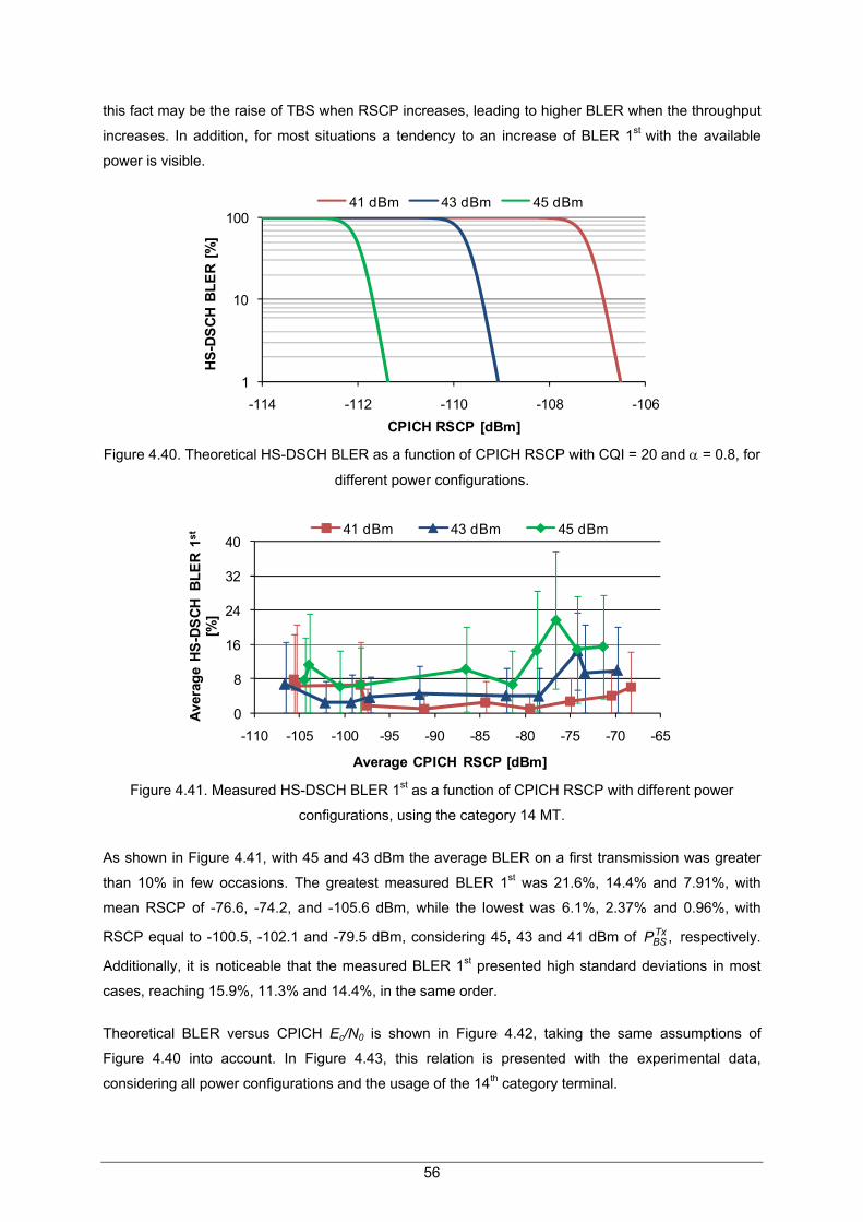
this fact may be the raise of TBS when RSCP increases, leading to higher BLER when the throughput
increases. In addition, for most situations a tendency to an increase of BLER 1st with the available
power is visible.
1
10
100
-114 -112 -110 -108 -106
HS-
DSCH
BLE
R [%
]
CPICH RSCP [dBm]
41 dBm 43 dBm 45 dBm
Figure 4.40. Theoretical HS-DSCH BLER as a function of CPICH RSCP with CQI = 20 and α = 0.8, for
different power configurations.
0
8
16
24
32
40
-110 -105 -100 -95 -90 -85 -80 -75 -70 -65
Aver
age
HS-D
SCH
BLE
R 1s
t
[%]
Average CPICH RSCP [dBm]
41 dBm 43 dBm 45 dBm
Figure 4.41. Measured HS-DSCH BLER 1st as a function of CPICH RSCP with different power
configurations, using the category 14 MT.
As shown in Figure 4.41, with 45 and 43 dBm the average BLER on a first transmission was greater
than 10% in few occasions. The greatest measured BLER 1st was 21.6%, 14.4% and 7.91%, with
mean RSCP of -76.6, -74.2, and -105.6 dBm, while the lowest was 6.1%, 2.37% and 0.96%, with
RSCP equal to -100.5, -102.1 and -79.5 dBm, considering 45, 43 and 41 dBm of respectively.
Additionally, it is noticeable that the measured BLER 1st presented high standard deviations in most
cases, reaching 15.9%, 11.3% and 14.4%, in the same order.
,TxBSP
Theoretical BLER versus CPICH Ec/N0 is shown in Figure 4.42, taking the same assumptions of
Figure 4.40 into account. In Figure 4.43, this relation is presented with the experimental data,
considering all power configurations and the usage of the 14th category terminal.
56

1
10
100
-18 -17 -16 -15 -14 -13 -12
HS-D
SCH
BLE
R [%
]
CPICH Ec/N0 [dB]
41 dBm 43 dBm 45 dBm
Figure 4.42. Theoretical HS-DSCH BLER as a function of CPICH Ec/N0 with CQI = 20 and α = 0.8, for
different power configurations.
The model sets that, for a given Ec/N0 greater than -17 dB, the lower the available power, the greater
the resultant BLER. Note that the theoretical HS-DSCH BLER is 10% for Ec/N0 approximately -16.9,
-14.8 and -12.8 dB, considering transmit power of 45, 43 and 41 dBm, in that order. In Figure 4.43,
one shows that the highest obtained BLER was reached for an average CPICH Ec/N0 equal to -15.8,
-14.4 and -17.3 dB, while the minimum BLER was obtained for -17.9, -17.4 and -11.4 dB of Ec/N0, with
equal to 45, 43 and 41 dBm, respectively. TxBSP
0
8
16
24
32
40
-19 -18 -17 -16 -15 -14 -13 -12 -11
Ave
rage
HS-
DSC
H BL
ER 1
st
[%]
Average CPICH Ec/N0 [dB]
41 dBm 43 dBm 45 dBm
Figure 4.43. Measured HS-DSCH BLER 1st as a function of CPICH Ec/N0 for different power
configurations, using the category 14 MT.
HS-DSCH BLER on a first transmission as a function of CQI using the 15 codes MT for all power
configurations is presented, Figure 4.44. Again, it should be noted that the greatest BLER values were
achieved for CQI higher than 24, in the 45 and 43 dBm configurations.
One can conclude that the results are not in accordance with the model. The latter expects the
decrease of the BLER with the increase of RSCP, Ec/N0 and CQI, while the former present the
opposite trend, with 45 and 43 dBm of It was also shown that average BLER on first .TxBSP
57

transmission reached the highest values for the maximum Node B available power.
0
8
16
24
32
40
8 10 12 14 16 18 20 22 24 26 28
Ave
rage
HS
-DS
CH B
LER
1st
[%]
Average CQI
41 dBm 43 dBm 45 dBm
Figure 4.44. Measured HS-DSCH BLER 1st as a function of CQI for different power configurations,
using the category 14 MT.
4.3 HSPA+ UL
In this section, one presents the comparison between the HSPA+ UL measurements results and the
theoretical models described in Chapter 3. The parameters addressed are E-DCH throughput, MT
transmit power and E-DCH BLER.
4.3.1 E-DCH Throughput
E-DCH throughput as a function of CPICH RSCP is presented, considering theoretical and
experimental data, for both 10 and 2 ms TTIs, Figure 4.45. As mentioned in the previous chapter, the
theoretical throughput is obtained taking the measured MT transmit power into account.
In Figure 4.45, one shows that the average throughput with 10 ms TTI was almost constant for RSCP
greater than -100 dBm, not exceeding 0.9 Mbps. On the contrary, with a TTI of 2 ms there was an
increase of the mean throughput as the radio channel conditions became more favourable, being
1.76 Mbps with average RSCP equal to -103.6 dBm to reach 4.27 Mbps with an RSCP of -64.9 dBm.
Moreover, the variation of data rate is perceptible on standard deviations, the largest being 0.23 and
0.75 Mbps for 10 and 2 ms TTIs, correspondingly. It is noticeable that the average data do not differ
significantly from the models, obtaining 31.2% and 21.4% of relative mean error, with standard
deviation of 22.9% and 29.6% considering 10 and 2 ms TTIs, respectively.
E-DCH throughput as a function of CPICH RSCP with a TTI of 10 ms, considering all data collected in
the measurements, is shown, Figure 4.46. In Figure 4.47, one presents the theoretical throughput
58

based on measured MT transmit power. Equivalent analysis with 2 ms TTI is also shown, Figure 4.48
and Figure 4.49.
0
1
2
3
4
5
-115 -110 -105 -100 -95 -90 -85 -80 -75 -70 -65 -60
E-D
CH T
hrou
ghpu
t [M
bps]
CPICH RSCP [dBm]
10 ms Theoretical 10 ms Measured2 ms Theoretical 2 ms Measured
Figure 4.45. Theoretical and measured E-DCH throughputs as a function of CPICH RSCP,
considering both TTIs.
Figure 4.46. Measured E-DCH throughput as a function of CPICH RSCP with 10 ms TTI.
Figure 4.47. Theoretical E-DCH throughput as a function of CPICH RSCP with 10 ms TTI.
With TTI equal to 10 ms, it is noticeable the great variation of throughput, both experimental and
59

theoretical. In both cases, the peak throughput (1.45 and 1.6 Mbps, considering measured and
expected value, respectively) is achieved for CPICH RSCP higher than -105 dBm. One obtained a
correlation factor of 0.333 and the RMSE is 0.435 Mbps, consistent with the results of the analysis
with average values. Additionally, one can observe several samples of E-DCH data rate equal to zero,
which also happened with 2 ms TTI, due to the fact that some packets were discarded when the buffer
reached its pole capacity.
Figure 4.48. Measured E-DCH throughput as a function of CPICH RSCP with 2 ms TTI.
Figure 4.49. Theoretical E-DCH throughput as a function of CPICH RSCP with 2 ms TTI.
In Figure 4.48 and Figure 4.49, one can observe a trend to an increase of E-DCH throughput with
RSCP, especially with RSCP between -120 and -95 dBm. Note that for RSCP lower than -100 dBm,
the maximum throughput was approximately 4 Mbps, while the peak throughput (measured 5.32 Mbps
and expected 5.15 Mbps) was reached for RSCP greater than -95 dBm. Still, the correlation factor is
0.444. In addition, the expected data rate is higher than the measured one in 66.6% of the samples,
which indicates that the theoretical performance was not achieved in the majority of occasions, with
the RMSE being 1.35 Mbps.
In conclusion, it was shown that the average E-DCH throughput was almost constant for TTI of 10 ms,
not surpassing 0.9 Mbps, while in the 2 ms TTI case it increased with CPICH RSCP, reaching 4.27
60
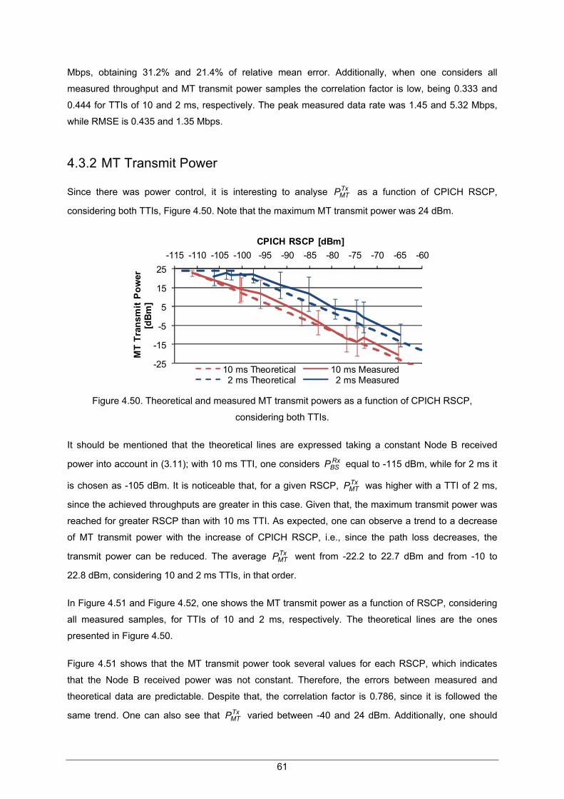
Mbps, obtaining 31.2% and 21.4% of relative mean error. Additionally, when one considers all
measured throughput and MT transmit power samples the correlation factor is low, being 0.333 and
0.444 for TTIs of 10 and 2 ms, respectively. The peak measured data rate was 1.45 and 5.32 Mbps,
while RMSE is 0.435 and 1.35 Mbps.
4.3.2 MT Transmit Power
Since there was power control, it is interesting to analyse as a function of CPICH RSCP,
considering both TTIs,
TxMTP
Figure 4.50. Note that the maximum MT transmit power was 24 dBm.
-25
-15
-5
5
15
25-115 -110 -105 -100 -95 -90 -85 -80 -75 -70 -65 -60
MT
Tran
smit
Pow
er
[dB
m]
CPICH RSCP [dBm]
10 ms Theoretical 10 ms Measured2 ms Theoretical 2 ms Measured
Figure 4.50. Theoretical and measured MT transmit powers as a function of CPICH RSCP,
considering both TTIs.
It should be mentioned that the theoretical lines are expressed taking a constant Node B received
power into account in (3.11); with 10 ms TTI, one considers equal to -115 dBm, while for 2 ms it
is chosen as -105 dBm. It is noticeable that, for a given RSCP, was higher with a TTI of 2 ms,
since the achieved throughputs are greater in this case. Given that, the maximum transmit power was
reached for greater RSCP than with 10 ms TTI. As expected, one can observe a trend to a decrease
of MT transmit power with the increase of CPICH RSCP, i.e., since the path loss decreases, the
transmit power can be reduced. The average went from -22.2 to 22.7 dBm and from -10 to
22.8 dBm, considering 10 and 2 ms TTIs, in that order.
RxBSP
PTxMT
TxMTP
In Figure 4.51 and Figure 4.52, one shows the MT transmit power as a function of RSCP, considering
all measured samples, for TTIs of 10 and 2 ms, respectively. The theoretical lines are the ones
presented in Figure 4.50.
Figure 4.51 shows that the MT transmit power took several values for each RSCP, which indicates
that the Node B received power was not constant. Therefore, the errors between measured and
theoretical data are predictable. Despite that, the correlation factor is 0.786, since it is followed the
same trend. One can also see that varied between -40 and 24 dBm. Additionally, one should TxMTP
61

mention that the experimental transmit power is higher than expected (considering -115 dBm of )
in 67.7% of the samples, so, in these cases, the received power was greater than -115 dBm.
RxBSP
Figure 4.51. MT transmit power as a function of CPICH RSCP with 10 ms TTI.
Figure 4.52. MT transmit power as a function of CPICH RSCP with 2 ms TTI.
Figure 4.52 also denotes that the Node B received power was not constant (as considered). In fact,
was higher than -105 dBm in 68.9% of the time, considering measured and CPICH RSCP.
Again, one can observe a trend to a decrease of MT transmit power, from 24 to -33 dBm, with
increase of RSCP, i.e., as the radio channel conditions become more favourable. In this situation the
correlation factor is 0.732.
RxBSP Tx
MTP
To summarise, it was shown that the average measured was higher for the lowest TTI case. It
was also noticeable the high correlation between measured and expected data, even considering fixed
TxMTP
.RxBSP
62

63
4.3.3 E-DCH BLER
In Figure 4.53, one presents the measured E-DCH BLER on a first transmission as a function of
CPICH RSCP, for both TTIs.
0
5
10
15
20
25
-115 -110 -105 -100 -95 -90 -85 -80 -75 -70 -65 -60
Aver
age
E-D
CH B
LER
1st[%
]
Average CPICH RSCP [dBm]
10 ms 2 ms
Figure 4.53. Measured E-DCH BLER 1st as a function of CPICH RSCP, considering both TTIs.
Figure 4.53 shows that the average E-DCH BLER 1st did not exceed 1.58% with 10 ms TTI, while it
reached 8.52% for TTI of 2 ms. In addition, standard deviations were also greater with the smallest
TTI, being the maximum deviation 3.89% and 14.42%, for 10 and 2 ms, respectively. It is noticeable
that average BLER was almost constant in the 10 ms TTI case, whereas with 2 ms it was greater with
average RSCP of -91.5 and -64.9 dBm. These results can be justified by the fact that the throughput is
higher with TTI of 2 ms, leading to lower data coding and, consequently, greater error probability.

64

65
Chapter 5
Conclusions 5 Conclusions
In this chapter, the main conclusions of this thesis are pointed out, as well as some future work
suggestions.
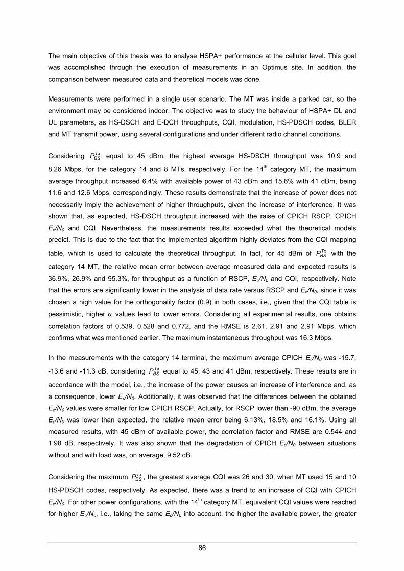
The main objective of this thesis was to analyse HSPA+ performance at the cellular level. This goal
was accomplished through the execution of measurements in an Optimus site. In addition, the
comparison between measured data and theoretical models was done.
Measurements were performed in a single user scenario. The MT was inside a parked car, so the
environment may be considered indoor. The objective was to study the behaviour of HSPA+ DL and
UL parameters, as HS-DSCH and E-DCH throughputs, CQI, modulation, HS-PDSCH codes, BLER
and MT transmit power, using several configurations and under different radio channel conditions.
Considering equal to 45 dBm, the highest average HS-DSCH throughput was 10.9 and
8.26 Mbps, for the category 14 and 8 MTs, respectively. For the 14th category MT, the maximum
average throughput increased 6.4% with available power of 43 dBm and 15.6% with 41 dBm, being
11.6 and 12.6 Mbps, correspondingly. These results demonstrate that the increase of power does not
necessarily imply the achievement of higher throughputs, given the increase of interference. It was
shown that, as expected, HS-DSCH throughput increased with the raise of CPICH RSCP, CPICH
Ec/N0 and CQI. Nevertheless, the measurements results exceeded what the theoretical models
predict. This is due to the fact that the implemented algorithm highly deviates from the CQI mapping
table, which is used to calculate the theoretical throughput. In fact, for 45 dBm of with the
category 14 MT, the relative mean error between average measured data and expected results is
36.9%, 26.9% and 95.3%, for throughput as a function of RSCP, Ec/N0 and CQI, respectively. Note
that the errors are significantly lower in the analysis of data rate versus RSCP and Ec/N0, since it was
chosen a high value for the orthogonality factor (0.9) in both cases, i.e., given that the CQI table is
pessimistic, higher α values lead to lower errors. Considering all experimental results, one obtains
correlation factors of 0.539, 0.528 and 0.772, and the RMSE is 2.61, 2.91 and 2.91 Mbps, which
confirms what was mentioned earlier. The maximum instantaneous throughput was 16.3 Mbps.
TxBSP
TxBSP
In the measurements with the category 14 terminal, the maximum average CPICH Ec/N0 was -15.7,
-13.6 and -11.3 dB, considering equal to 45, 43 and 41 dBm, respectively. These results are in
accordance with the model, i.e., the increase of the power causes an increase of interference and, as
a consequence, lower Ec/N0. Additionally, it was observed that the differences between the obtained
Ec/N0 values were smaller for low CPICH RSCP. Actually, for RSCP lower than -90 dBm, the average
Ec/N0 was lower than expected, the relative mean error being 6.13%, 18.5% and 16.1%. Using all
measured results, with 45 dBm of available power, the correlation factor and RMSE are 0.544 and
1.98 dB, respectively. It was also shown that the degradation of CPICH Ec/N0 between situations
without and with load was, on average, 9.52 dB.
TxBSP
Considering the maximum , the greatest average CQI was 26 and 30, when MT used 15 and 10
HS-PDSCH codes, respectively. As expected, there was a trend to an increase of CQI with CPICH
Ec/N0. For other power configurations, with the 14th category MT, equivalent CQI values were reached
for higher Ec/N0, i.e., taking the same Ec/N0 into account, the higher the available power, the greater
TxBSP
66
the CQI. Again, a constant orthogonality factor (0.8) was considered in the theoretical model, the
relative mean error being 8.92%, 11.4% and 10.1%, for equal to 45, 43 and 41 dBm, in that
order. In the analysis with all collected data and 45 dBm of available power, one obtains a correlation
factor of 0.639 and an RMSE of 3. Summarising, the adopted model proved to be a good
approximation to the measured results.
TxBSP
Regarding the modulation ratio, for the 8th category MT with 45 dBm of , the average usage of
16QAM reached 100% for mean CQI greater than 21, with CPICH RSCP and CPICH Ec/N0 higher
than 83.8 dBm and -16.2 dB, respectively. For the 14th category device, the maximum 64QAM usage
was 36.5%, with an average CQI of 26, RSCP of -74.3 dBm and Ec/N0 equal to -15.8 dB. Note that the
theoretical modulation ratio is 100% or 0%, whether the modulation is used or not, while the
experimental results correspond to mean values during the measurements. The relative mean error for
modulation ratio as a function of CQI, RSCP and Ec/N0 is 16.1%, 36% and 7.8%, in that order,
considering the category 8 MT, and 20%, 47.2% and 7.8%, using the category 14 MT. It was shown
that the model based on the CQI mapping tables, being optimistic, is a good approximation of the
measured modulation ratio as a function of CQI. Since this model is also used in the remaining
analysis, the smallest errors are obtained with low orthogonality factor values (0.1 and 0.3 for RSCP
and Ec/N0, respectively). Nevertheless, considering these α values, the 64QAM’s theoretical curves
are quite different from the measured ones, given that the orthogonality factor was not constant during
the measurements.
TxBSP
The number of used HS-PDSCH codes was another parameter analysed. Using the category 8 MT,
10 HS-PDSCH codes were used for CQI greater than 16, while the CQI mapping table only defines
the usage of 10 codes for CQI higher than or equal to 25. In the measurements with the category 14
MT, 15 codes were used with CQI greater than 22, whereas, in theory, the usage of the maximum
number of codes is defined only for CQI equal to 30. The relative mean error is 67.5% and 143%,
using the category 8 and 14 MTs, respectively. It should be mentioned that even for low CPICH RSCP
values, i.e., under unfavourable radio conditions, the average usage of the greatest number of codes
varied from 66.5% to 88.3% and from 47.5% to 85%, using 10 and 15 codes, respectively, suggesting
that the implemented algorithm defines the usage of the maximum number of HS-PDSCH codes
whenever possible. These results are representative of the discrepancies between model and
experimental data, revealing why the theoretical throughput is generally lower than the measured.
During the measurements with the 14th category terminal, one observed a trend to an increase of the
average HS-DSCH BLER on a first transmission with the available power. In addition, with 45 and 43
dBm of the average BLER 1st increased with the raise of CPICH RSCP, CPICH Ec/N0 and CQI.
This is due to the increase of TBS, achieving higher throughput as well as greater BLER. The greatest
experimental BLER 1st was 21.6%, 14.4% and 7.91%, while the lowest was 6.1%, 2.37% and 0.96%,
considering 45, 43 and 41 dBm of respectively.
,TxBSP
,TxBSP
67

68
The average E-DCH throughput was almost constant with 10 ms TTI for CPICH RSCP greater than
-100 dBm, while with a 2 ms TTI there was an increase of throughput with RSCP. The average data
rate ranged between 0.27 and 0.90 Mbps, and 1.76 and 4.27 Mbps, considering 10 and 2 ms TTI, in
that order. Experimental results do not differ significantly from the models; one obtains 31.2% and
21.4% of relative mean error. Considering all available data, it was noticeable the wide variation of
throughput, with some samples equal to zero, due to the fact that there were packets discarded when
the buffer reached its pole capacity. The peak instantaneous E-DCH throughput was 1.45 and 5.32
Mbps, for 10 and 2 ms TTIs, respectively. With a TTI of 10 ms, one obtains a correlation factor of
0.333 and the RMSE is 0.435 Mbps, while with the smallest TTI the correlation factor and RMSE are
0.444 and 1.35 Mbps, correspondingly.
It was observed a trend to a decrease of MT transmit power with the increase of CPICH RSCP, i.e.,
when the path loss decreased. The average varied between -22.2 and 22.7 dBm, and between
-10 and -22.8 dBm, considering 10 and 2 ms TTI, in that order. Given the same RSCP, the average
was greater with the lowest TTI, since the achieved throughputs were higher. Moreover,
considering -115 and -105 dBm of Node B received power for 10 and 2 ms TTIs, the correlation factor
is 0.786 and 0.732, considering fixed . The instantaneous MT transmit power ranged from -40 to
24 dBm with a 10 ms TTI, and from -33 to 24 dBm with a 2 ms TTI.
TxMTP
TxMTP
RxBSP
The average E-DCH BLER 1st did not exceed 1.58% with 10 ms TTI, while it reached 8.52% for TTI of
2 ms. UL BLER on first transmission was almost constant in the 10 ms TTI case, whereas with 2 ms
TTI presented higher values with mean CPICH RSCP of -91.5 and -64.9 dBm. These results can be
explained by the fact that the throughput is higher with TTI of 2 ms, leading to lower data coding and,
consequently, greater error probability.
For future work, it is suggested the study of HSPA+ performance with the introduction of MIMO and
16QAM in UL, by performing measurements with these capabilities, and comparing the measured
data with theoretical models. Other suggestion is to carry out measurements in different environments.
Also the impact of introducing more users in the same cell, it is interesting to analyse. One could also
suggest the study of LTE performance at the cellular level, both in single and multiple user scenarios,
by developing a simulator.

69
Annex A – MIMO
Annex A – MIMO
A brief overview over the general and capacity aspects of MIMO is presented in this annex.
MIMO takes advantage of the multipath propagation, where the Receiver (Rx) antenna is reached by
many copies of the transmitted signal. The difference in each component propagation path results in
diversity of Time of Arrival (ToA), Angle of Arrival (AoA), signal amplitude and phase. With the purpose
of achieving a better performance, MIMO systems take advantage of all arriving arrays [Maćk07]. It
exploits independently the transmission between the Transmitter (Tx) and Rx antennas.
The MIMO scheme, which is the result of parallel deployment of several space-separated antennas at
input and output, improves not only BER performance but also causes an increase of channel capacity
[Maćk07]. Even so, the capacity in such system strongly depends on the propagation conditions in the
radio channel and can vary considerably [Dziu04].
A MIMO system is composed of NT Tx antennas and NR Rx antennas, Figure A.1.
Figure A.1. MIMO scheme (extracted from [Maćk07]).
ξ is the mean correlation between links in a MIMO system, and is defined by:
( )(∑ ∑ ∑ ∑= = = =
ξ=ξ T R T RN
k
N
l
N
m
N
n mnklRT
hhNN 1 1 1 12
,1 ) (A.1)
where:
• hkl is a Channel Impulse Response (CIR) between signal from the lth Tx antenna to the kth Rx
antenna.

According to the general principles of information theory, the capacity of the radio channel is bounded
by Shannon’s rule, [Proa01], which represents the capacity of a Single Input Single Output (SISO)
system, usually taken as a reference:
)1(log2[bps/hz] NSISOC ρ+= (A.2)
where:
• CSISO is the capacity of a radio channel;
• ρN is the SNR.
In an ideal case, it can be shown that the channel capacity grows linearly with the number of Tx and
Rx antennas [ECGF05]. In MIMO systems is possible to establish multiple parallel subchannels, which
operate simultaneously at the same time and on the same frequency band. The theoretical capacity of
such a system has been presented in [FoGa98]:
⎪⎭
⎪⎬⎫
⎪⎩
⎪⎨⎧
⎥⎦
⎤⎢⎣
⎡ ρ+= H
nnRN HHIT
NMIMO N
C detlog2[bps/Hz] (A.3)
where:
• INR is the NR dimensional identity matrix;
• ρN is defined at each Rx antenna as:
bPP
noise
totalN =ρ (A.4)
where:
• Pnoise is the noise power at the Rx antenna.
• Hn is the normalised channel transfer matrix related to T as:
bTHn = (A.5)
• T is the non-normalised channel transfer matrix, containing the channel transfer gains for each
pair of antennas;
• b is defined as:
[ ] 2
1 1
22 1 ∑ ∑= === R TN
m
N
n mnRT
TNN
Rb T (A.6)
It is possible to obtain the upper and lower bounds for capacity from (A.3) since the correlation varies
between zero and one. The maximum capacity is achieved if there is no correlation between parallel
paths (ξ=0):
)1(log);min( 2)0(T
NNRTMIMO NNC ρ
=ξ += (A.7)
70

On the other hand, when all subchannels are totally correlated (ξ=1), the minimum capacity of a MIMO
channel occurs:
));min(1(log2)1(T
NNRTMIMO NNC ρ
=ξ += (A.8)
When the channel is known at the Tx, meaning the correlation between subchannels is known at the
Tx, the waterfilling power distribution can be performed. In specified conditions this allows to operate
with the maximum achievable capacity.
The Relative MIMO Gain (RMG) can be defined as the relation between the capacities of a MIMO
system related to the SISO one, [KuCo08]:
SISO
MIMOSM C
CG = (A.9)
71

Annex B – Link Budget
Annex B – Link Budget The presented link budget is based on the Release 99 one, described in detail in [CoLa06] and
[Sant04], adapted to HSPA+.
The path loss can be calculated by [Corr06]:
[dBi][dBm][dBm][dBi][dBm][dBi][dBm][dB] rrrrttP GPEIRPGPGPL +−=+−+= (B.1)
where:
• Lp is the path loss;
• Pt is the transmitting power at antenna port;
• Gt is the transmitting antenna gain;
• Pr is the available receiving power at antenna port;
• Gr is the receiving antenna gain.
If diversity is used, Gr in (B.1) is replaced by:
[dB][dBi][dB] divrrdiv GGG += (B.2)
where:
• Gdiv represents the diversity gain.
The Equivalent Isotropic Radiated Power (EIRP) can be calculated for DL by (B.3), and for UL by
(B.4).
( ) [dBi][dB][dBm]&[dBm] tcCSt GLPPEIRP +−−= (B.3)
( ) [dB][dBi][dB][dBm]&[dBm] MHAtuCSt GGLPPEIRP −+−−= (B.4)
where:
• Lc are the cable losses between transmitter and antenna;
• Lu are user losses;
• GMHA is the masthead amplifier gain;
• PS&C is the signalling and control power.
The received power can be calculated by (B.5) for DL and (B.6) for UL:
[dB][dBm][dBm] urRx LPP −= (B.5)
72

[dB][dBm][dBm] crRx LPP −= (B.6)
where:
• PRx is the received power at receiver input.
The HSPA+ receiver sensitivity can be approximated by:
[dB][dB][dBm][dBm]min INpRx GNP ρ+−= (B.7)
where:
• minRxP is the receiver sensitivity;
• N is the total noise power given by (B.8);
• Gp is the processing gain, Table B.1;
• ρIN is the signal to noise ratio, Table B.1;
• Rb is the data rate;
• Rc is the WCDMA chip rate;
• Ec/N0 is the energy per chip to noise power spectral density ratio.
Table B.1. HSPA+ processing gain and SNR definition.
System Processing Gain SNR/SINR HSPA+ DL Fixed and equal to 16 (SF16) ρIN
HSPA+ UL Rc/Rb Ec/N0
The total noise power is:
[dB][dB][Hz][dBm] )log(10174 IMFfN ++Δ⋅+−= (B.8)
where:
• Δf is the signal bandwidth;
• F is the receiver’s noise figure;
• MI is the interference margin.
For HSPA+ UL, the metric used for SNR is the Ec/N0. The E-DPDCH throughput is a continuous
function of the Eb/N0 at the Node B.
The Eb/N0 is necessary being obtained from interpolation of Ec/N0:
[dB][dB]0[dB]0 pcb GNENE += (B.9)
In HSPA+ UL, manipulating (B.7) and (B.9), the Ec/N0 for a certain user’s distance is given by:
73
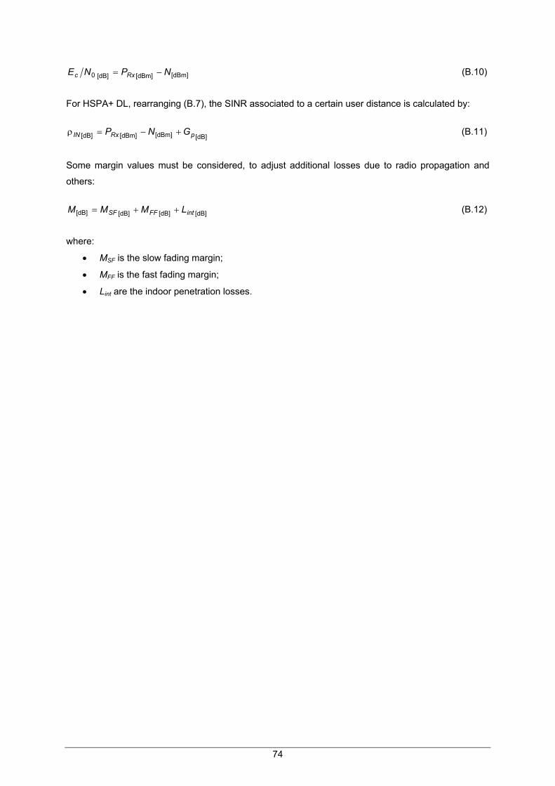
[dBm][dBm][dB]0 NPNE Rxc −= (B.10)
For HSPA+ DL, rearranging (B.7), the SINR associated to a certain user distance is calculated by:
[dB][dBm][dBm][dB] pRxIN GNP +−=ρ (B.11)
Some margin values must be considered, to adjust additional losses due to radio propagation and
others:
[dB][dB][dB][dB] intFFSF LMMM ++= (B.12)
where:
• MSF is the slow fading margin;
• MFF is the fast fading margin;
• Lint are the indoor penetration losses.
74

Annex C – HSPA+ DL Additional Results
Annex C – HSPA+ DL Additional
Results Modulation ratio as a function of CPICH RSCP is presented for the 8th category MT, considering
equal to 43 and 41 dBm,
TxBSP
Figure C.1 and Figure C.2. The analysis regarding the category 14 terminal
is also shown, Figure C.3 and Figure C.4, for 43 and 41 dBm, respectively.
0
50
100
-115 -110 -105 -100 -95 -90 -85 -80 -75 -70
Mod
ulat
ion
Ratio
[%
]
CPICH RSCP [dBm]
QPSK Theoretical QPSK Measured16 QAM Theoretical 16QAM Measured
Figure C.1. Theoretical and measured modulation ratios as a function of CPICH RSCP for the
category 8 MT, with .dBm43=TxBSP
0
50
100
-115 -110 -105 -100 -95 -90 -85 -80 -75 -70
Mod
ulat
ion
Ratio
[%
]
CPICH RSCP [dBm]
QPSK Theoretical QPSK Measured16 QAM Theoretical 16QAM Measured
Figure C.2. Theoretical and measured modulation ratios as a function of CPICH RSCP for the
category 8 MT, with .dBm41=TxBSP
75

0
50
100
-115 -110 -105 -100 -95 -90 -85 -80 -75 -70 -65
Mod
ulat
ion
Ratio
[%]
CPICH RSCP [dBm]
QPSK Theoretical QPSK Measured16QAM Theoretical 16QAM Measured64QAM Theoretical 64QAM Measured
Figure C.3. Theoretical and measured modulation ratios as a function of CPICH RSCP for the
category 14 MT, with .dBm43=TxBSP
0
50
100
-115 -110 -105 -100 -95 -90 -85 -80 -75 -70 -65
Mod
ulat
ion
Rat
io [%
]
CPICH RSCP [dBm]
QPSK Theoretical QPSK Measured16QAM Theoretical 16QAM Measured64QAM Theoretical 64QAM Measured
Figure C.4. Theoretical and measured modulation ratios as a function of CPICH RSCP for the
category 14 MT, with .dBm41=TxBSP
In Figure C.5, one shows the modulation ratio versus Ec/N0 for the category 8 MT, with equal to
43 dBm. Results concerning the minimum available power are also presented,
TxBSP
Figure C.6. In addition,
the same analysis for the 14th category MT is done, Figure C.7 and Figure C.8.
In Figure C.9 and Figure C.10, one presents the modulation ratio as a function of CQI, for the terminal
that only uses QPSK and 16QAM, considering the power configurations with 43 and 41 dBm,
respectively. Again, results regarding the usage of 64QAM are also shown, Figure C.11 and Figure
C.12.
76

0
50
100
-19 -18 -17 -16 -15 -14 -13
Mod
ulat
ion
Ratio
[%]
CPICH Ec/N0 [dB]
QPSK Theoretical QPSK Measured16QAM Theoretical 16QAM Measured
Figure C.5. Theoretical and measured modulation ratios as a function of CPICH Ec/N0 for the category
8 MT, with .dBm43=TxBSP
0
50
100
-17 -16 -15 -14 -13 -12 -11
Mod
ulat
ion
Ratio
[%]
CPICH Ec/N0 [dB]
QPSK Theoretical QPSK Measured16QAM Theoretical 16QAM Measured
Figure C.6. Theoretical and measured modulation ratios as a function of CPICH Ec/N0 for the category
8 MT, with .dBm41=TxBSP
0
50
100
-16 -14 -12 -10 -8 -6
Mod
ulat
ion
Rat
io [%
]
CPICH Ec/N0 [dB]
QPSK Theoretical QPSK Measured16QAM Theoretical 16QAM Measured 64QAM Theoretical 64QAM Measured
Figure C.7. Theoretical and measured modulation ratios as a function of CPICH Ec/N0 for the category
14 MT, with .dBm43=TxBSP
77
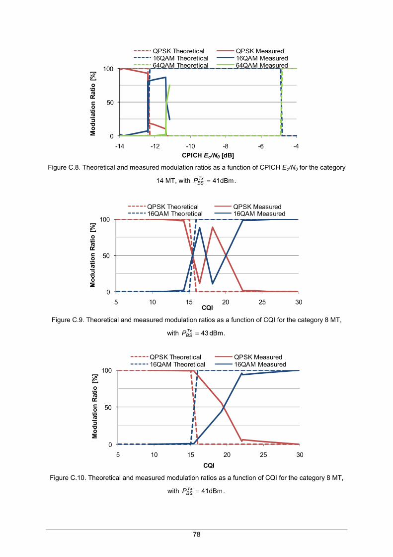
78
0
50
100
-14 -12 -10 -8 -6 -4
Mod
ulat
ion
Ratio
[%]
CPICH Ec/N0 [dB]
QPSK Theoretical QPSK Measured16QAM Theoretical 16QAM Measured64QAM Theoretical 64QAM Measured
Figure C.8. Theoretical and measured modulation ratios as a function of CPICH Ec/N0 for the category
14 MT, with .dBm41=TxBSP
0
50
100
5 10 15 20 25 3
Mod
ulat
ion
Ratio
[%]
CQI0
QPSK Theoretical QPSK Measured16QAM Theoretical 16QAM Measured
Figure C.9. Theoretical and measured modulation ratios as a function of CQI for the category 8 MT,
with .dBm43=TxBSP
0
50
100
5 10 15 20 25 3
Mod
ulat
ion
Ratio
[%]
CQI0
QPSK Theoretical QPSK Measured16QAM Theoretical 16QAM Measured
Figure C.10. Theoretical and measured modulation ratios as a function of CQI for the category 8 MT,
with .dBm41=TxBSP
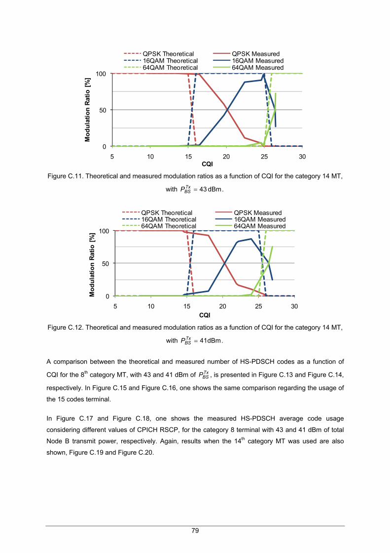
79
0
50
100
5 10 15 20 25 3
Mod
ulat
ion
Rat
io [
%]
CQI0
QPSK Theoretical QPSK Measured16QAM Theoretical 16QAM Measured64QAM Theoretical 64QAM Measured
Figure C.11. Theoretical and measured modulation ratios as a function of CQI for the category 14 MT,
with .dBm43=TxBSP
0
50
100
5 10 15 20 25 3
Mod
ulat
ion
Ratio
[%
]
CQI0
QPSK Theoretical QPSK Measured16QAM Theoretical 16QAM Measured64QAM Theoretical 64QAM Measured
Figure C.12. Theoretical and measured modulation ratios as a function of CQI for the category 14 MT,
with .dBm41=TxBSP
A comparison between the theoretical and measured number of HS-PDSCH codes as a function of
CQI for the 8th category MT, with 43 and 41 dBm of , is presented in TxBSP Figure C.13 and Figure C.14,
respectively. In Figure C.15 and Figure C.16, one shows the same comparison regarding the usage of
the 15 codes terminal.
In Figure C.17 and Figure C.18, one shows the measured HS-PDSCH average code usage
considering different values of CPICH RSCP, for the category 8 terminal with 43 and 41 dBm of total
Node B transmit power, respectively. Again, results when the 14th category MT was used are also
shown, Figure C.19 and Figure C.20.

80
2
4
6
8
10
10 15 20 25 30
Num
ber
of H
S-P
DSC
H C
odes
CQI
Theoretical Measured
Figure C.13. Number of HS-PDSCH codes as a function of CQI with using the
category 8 MT, considering theoretical and measured data.
dBm,43=TxBSP
0
2
4
6
8
10
5 10 15 20 25 3
Num
ber o
f HS-
PDS
CH
Cod
es
CQI 0
Theoretical Measured
Figure C.14. Number of HS-PDSCH codes as a function of CQI with using the category
8 MT, considering theoretical and measured data.
dBm,41=TxBSP
3
5
7
9
11
13
15
10 15 20 25 30
Num
ber o
f HS
-PD
SCH
Code
s
CQI
Theoretical Measured
Figure C.15. Number of HS-PDSCH codes as a function of CQI with using the
category 14 MT, considering theoretical and measured data.
dBm,43=TxBSP

3
579
111315
10 15 20 25 30
Num
ber o
f HS-
PDS
CH
Code
s
CQI
Theoretical Measured
Figure C.16. Number of HS-PDSCH codes as a function of CQI with using the category
14 MT, considering theoretical and measured data.
dBm,41=TxBSP
0
20
40
60
80
100
-105.7 -102.5 -97.5
Ave
rage
HS-
PDS
CH C
ode
Usa
ge [%
]
Average CPICH RSCP [dBm]
2 4 6 8 10Number of HS-PDSCH codes
Figure C.17. Measured HS-PDSCH code usage as a function of CPICH RSCP with
considering the category 8 MT. dBm,43=TxBSP
0
20
40
60
80
100
-105.0 -104.1 -98.9 -96.3
Ave
rage
HS
-PDS
CH C
ode
Usa
ge [%
]
Average CPICH RSCP [dBm]
2 4 6 8 10Number of HS-PDSCH codes
Figure C.18. Measured HS-PDSCH code usage as a function of CPICH RSCP with
considering the category 8 MT. dBm,41=TxBSP
81

0
20
40
60
80
100
-106.6 -102.1 -99.2 -97.2
Ave
rage
HS-
PDS
CH C
ode
Usag
e [%
]
Average CPICH RSCP [dBm]
2 3 4 6 7 10 12 15Number of HS-PDSCH codes
Figure C.19. Measured HS-PDSCH code usage as a function of CPICH RSCP with
considering the category 14 MT. dBm,43=TxBSP
0
20
40
60
80
-105.6 -105.4 -98.2 -97.5
Ave
rage
HS-
PDS
CH C
ode
Usag
e [%
]
Average CPICH RSCP [dBm]
1 2 3 4 5 7 9 12 13 15Number of HS-PDSCHcodes
Figure C.20. Measured HS-PDSCH code usage as a function of CPICH RSCP with
considering the category 14 MT. dBm,41=TxBSP
HS-DSCH BLER on first transmission as a function of CPICH RSCP, CPICH Ec/N0 and CQI, for the
category 8 MT, is presented, Figure C.21, Figure C.22 and Figure C.23, respectively.
0
8
16
24
32
40
-110 -105 -100 -95 -90 -85 -80 -75 -70 -65 -60
Aver
age
HS-D
SCH
BLE
R 1s
t [%
]
Average CPICH RSCP [dBm]
41 dBm 43 dBm 45 dBm
Figure C.21. Measured HS-DSCH BLER 1st as a function of CPICH RSCP for different power
configurations, using the category 8 MT.
82

0
8
16
24
32
40
-20 -18 -16 -14 -12 -10 -8
Aver
age
HS-
DSC
H B
LER
1s
t [%
]
Average CPICH Ec/N0 [dB]
41 dBm 43 dBm 45 dBm
Figure C.22. Measured HS-DSCH BLER 1st as a function of CPICH Ec/N0 for different power
configurations, using the category 8 MT.
0
8
16
24
32
40
8 10 12 14 16 18 20 22 24 26 28 30
Ave
rage
HS-
DSC
H BL
ER
1st [
%]
Average CQI
41 dBm 43 dBm 45 dBm
Figure C.23. Measured HS-DSCH BLER 1st as a function of CQI for different power configurations,
using the category 8 MT.
83

84
References
References [3GAM09] http://www.3gamericas.org/index.cfm?fuseaction=page&pageid=565, Set. 2009.
[3GPP02] 3GPP, Technical Specification Group - Radio Access Network Working, Revised CQI
Proposal, Motorola, Ericsson, Report R1-020675, Paris, France, Apr. 2002.
[3GPP08] 3GPP, Technical Specification Group Services and System Aspects, Service aspects;
Services and Service Capabilities (Release 9), Report TS 22.105, V9.0.0, Dec. 2008
(http://www.3gpp.org/ftp/Specs/html-info/22105.htm).
[3GPP09a] 3GPP, Technical Specification Group Radio Access Network, UE Radio Access
capabilities (Release 8), Report TS 25.306, V8.7.0, Jun. 2009
(http://www.3gpp.org/ftp/Specs/html-info/25306.htm).
[3GPP09b] 3GPP, Technical Specification Group Radio Access Network, Physical layer -
Measurements (FDD) (Release 8), Report TS 25.215, V8.3.0, Mar. 2009
(http://www.3gpp.org/ftp/Specs/html-info/25215.htm).
[3GPP09c] 3GPP, Technical Specification Group Radio Access Network, Physical Layer Procedures
(FDD) (Release 8), Report TS 25.214, V8.6.0, May 2009
(http://www.3gpp.org/ftp/Specs/html-info/25214.htm).
[3GPP09d] 3GPP, Technical Specification Group Radio Access Network, User Equipment (UE)
conformance specification; Radio transmission and reception (FDD); Part 1:
Conformance specification (Release 8), Report TS 34.121-1, V8.7.0, Jun. 2009
(http://www.3gpp.org/ftp/Specs/html-info/34121-1.htm).
[Asco09] http://www.ascom.com/en/index/products-solutions/technology-platforms/platform/tems/
solutionloader.htm, Oct. 2009.
[BBSS04] Brouwer,F., Bruin,I., Silva,J., Souto,N., Cercas,F. and Correia,A., “Usage of Link-Level
Performance Indicators for HSDPA Network-Level Simulations in E-UMTS”, in Proc. of
ISSSTA-2004 - IEEE International Symposium on Spread Spectrum Techniques and
Applications, Sydney, Australia, Sep. 2004.
[BEGG08] Bergman,J., Ericson,M., Gerstenberger,D., Göransson,B., Peisa,J. and Wager,S., HSPA
Evolution – Boosting the performance of mobile broadband access, Ericsson Review,
Nº1, 2008.
85

[CoLa06] Costa,P. and Ladeira,D., Planning of UMTS Cellular Networks for Data Services Based
on HSDPA (in Portuguese), Graduation Thesis, Instituto Superior Técnico, Lisbon,
Portugal, Jun. 2006.
[Corr06] Correia,L.M., Mobile Communication Systems – Course Notes, IST-TUL, Lisbon,
Portugal, Mar. 2006.
[Dziu04] Dziunikowski,W., Multiple-Input Multiple-Output (MIMO) Antenna Systems, in Chandran,
S. (ed.), Adaptive Antenna Arrays, Springer, Berlin, Germany, 2004.
[ECGF05] El Zein,G., Cosquer,R., Guillet,J., Farhat,H. and Sagnard,F., “Characterisation and
Modeling of the MIMO Propagation Channel: An Overview”, in Proc. of European
Conference Wireless Technology, Paris, France, Oct. 2005.
[Eric09] White Paper, Accelerating global development with mobile broadband, Ericsson
Research, Feb. 2009 (http://www.ericsson.com/technology/whitepapers/acc-global-dev-
with-mbb.pdf).
[GoEa09] http://earth.google.com/, Sep. 2009.
[GSMW09] http://gsmworld.com/newsroom/press-releases/2009/2521.htm#nav-6, Sep. 2009.
[HGMT05] Hagerman,B., Gunnarsson,F., Murai,H., Tadenuma,M. and Karlsson,J., “WCDMA Uplink
Parallel Interference Cancellation - System Simulations and Prototype Field Trials”,
EURASIP Journal on Applied Signal Processing, Vol. 2005, Issue 11, Nov. 2005, pp.
1725-1735.
[HoTo04] Holma,H. and Toskala,A., WCDMA for UMTS – Radio Access For Third Generation
Mobile Communications, John Wiley & Sons, Chichester, UK, 2004.
[HoTo06] Holma,H. and Toskala,A., HSDPA/HSUPA for UMTS – High Speed Radio Access for
Mobile Communications, John Wiley & Sons, Chichester, UK, 2006.
[HoTo07] Holma,H. and Toskala,A., WCDMA for UMTS – HSPA Evolution and LTE (4th Edition),
John Wiley & Sons, Chichester, UK, 2007.
[HoTo09] Holma,H. and Toskala,A., LTE for UMTS – OFDMA and SC-FDMA Based Radio Access,
John Wiley & Sons, Chichester, UK, 2009.
[KuCo08] Kuipers,M. and Correia,L.M., "Modelling the Relative MIMO Gain", in Proc. of PIMRC’08 -
IEEE Personal, Indoor and Mobile Radio Communications, Cannes, France, Sep. 2008.
[Lope08] Lopes,J., Performance of UMTS/HSDPA/HSUPA at the Cellular Level, M.Sc. Thesis,
Instituto Superior Técnico, Lisbon, Portugal, Mar. 2008.
[Maćk07] Maćkowiak,M., Geometrically Based Multibounce MIMO Channel Models, M.Sc. Thesis,
86

87
Instituto Superior Técnico, Lisbon, Portugal, Sep. 2007.
[Moli05] Molisch,A.F., Wireless Communications, John Wiley & Sons, Chichester, UK, 2005.
[Opti09] Private Communication, Optimus, 2009.
[Pede05] Pedersen,K.I., “Quality Based HSDPA Access Algorithms”, in Proc of VTC Fall 2005 –
62nd IEEE Vehicular Technology Conference, Dallas, TX, USA, Sep. 2005.
[Preg08] Preguiça,R., Comparison between UMTS/HSPA+ and WiMax/IEEE 802.16e in Mobility
Scenarios, M.Sc. Thesis, Instituto Superior Técnico, Lisbon, Portugal, Sep. 2008.
[Proa01] Proakis,J.G., Digital Communications, MacGraw Hill, New York, NY, USA, 2001.
[Salv08] Salvado,L., UMTS/HSDPA comparison with WiMAX/IEEE 802.16e in mobility scenarios,
M.Sc. Thesis, Instituto Superior Técnico, Lisbon, Portugal, Fev. 2008.
[Sant04] Santo,L., UMTS Performance in Multi-Service Non-Uniform Traffic Networks, M.Sc.
Thesis, Instituto Superior Técnico, Lisbon, Portugal, Dec. 2004.