Data Mining: Datadatamining.rutgers.edu/teaching/fall2014/DM/lecture2.pdf · Data Mining: Data Dr....

Data Mining: Data

Dr. Hui XiongRutgers University

Introduction to Data Mining 1/2/2009 1

Outline

Attributes and Objects

Types of Data

Data Quality


Data Preprocessing

What is Data?

Collection of data objects and their attributes

An attribute is a property or Tid Ref nd Marital Ta able

Attributes

An attribute is a property or characteristic of an object

– Examples: eye color of a person, temperature, etc.

– Attribute is also known as variable, field, characteristic, or feature

Tid Refund MaritalStatus

Taxable Income Cheat

1 Yes Single 125K No

2 No Married 100K No

3 No Single 70K No

4 Yes Married 120K No

5 No Divorced 95K YesObj

ects

A collection of attributes describe an object

– Object is also known as record, point, case, sample, entity, or instance

5 No Divorced 95K Yes

6 No Married 60K No

7 Yes Divorced 220K No

8 No Single 85K Yes

9 No Married 75K No

10 No Single 90K Yes 10

O

Attribute Values

Attribute values are numbers or symbols assigned to an attribute for a particular object

Distinction between attributes and attribute values– Same attribute can be mapped to different attribute

valuesExample: height can be measured in feet or meters

– Different attributes can be mapped to the same set of


Different attributes can be mapped to the same set of values

Example: Attribute values for ID and age are integersBut properties of attribute values can be different

Measurement of Length

The way you measure an attribute may not match the attributes properties.

15 A

B2

3

7

8

10 4

B

C

D

This scale preserves the ordering and additive properties of length

This scale preserves only the ordering property of length

515

10 4

E

length.length.

Types of Attributes

There are different types of attributes– Nominal

Examples: ID numbers, eye color, zip codes– Ordinal

Examples: rankings (e.g., taste of potato chips on a scale from 1-10), grades, height in {tall, medium, short}

– Interval


Examples: calendar dates, temperatures in Celsius or Fahrenheit.

– RatioExamples: temperature in Kelvin, length, time, counts

Properties of Attribute Values

The type of an attribute depends on which of the following properties it possesses:

Di ti t– Distinctness: = ≠– Order: < >– Addition: + -– Multiplication: * /

N i l tt ib t di ti t


– Nominal attribute: distinctness– Ordinal attribute: distinctness & order– Interval attribute: distinctness, order & addition– Ratio attribute: all 4 properties

Difference Between Ratio and Interval

Is it physically meaningful to say that a temperature of 10 ° degrees twice that of 5° on – the Celsius scale?the Celsius scale?– the Fahrenheit scale?– the Kelvin scale?

Consider measuring the height above averageIf Bill’s height is three inches above average and


– If Bill s height is three inches above average and Bob’s height is six inches above average, then would we say that Bob is twice as tall as Bob?

– Is this situation analogous to that of temperature?

Attribute Type

Description

Examples

Operations

Nominal

Nominal attribute values only distinguish. (=, ≠)

zip codes, employee ID numbers, eye color, sex: {male, female}

mode, entropy, contingency correlation, χ2 test or

ical

ta

tive

Cat

egQ

ualit

Ordinal Ordinal attribute values also order objects. (<, >)

hardness of minerals, {good, better, best}, grades, street numbers

median, percentiles, rank correlation, run tests, sign tests

Interval For interval attributes, differences between values are

calendar dates, temperature in Celsius or Fahrenheit

mean, standard deviation, Pearson's correlation, t and er

ic

ativ

e

meaningful. (+, - ) F tests

Num

eQ

uant

it

Ratio For ratio variables, both differences and ratios are meaningful. (*, /)

temperature in Kelvin, monetary quantities, counts, age, mass, length, current

geometric mean, harmonic mean, percent variation

This categorization of attributes is due to S. S. Stevens

Attribute Type

Transformation

Comments

Nominal

Any permutation of values

If all employee ID numbers were reassigned, would it make any difference?

oric

al

ativ

e

Ordinal An order preserving change of An attribute encompassing

Cat

ego

Qua

lita Ordinal An order preserving change of

values, i.e., new_value = f(old_value) where f is a monotonic function

An attribute encompassing the notion of good, better best can be represented equally well by the values {1, 2, 3} or by { 0.5, 1, 0}.

Interval new_value =a * old_value + b where a and b are constants

Thus, the Fahrenheit and Celsius temperature scales differ in terms of where their zero value is and the size of am

eric

tit

ativ

e

zero value is and the size of a unit (degree). N

umQ

uant

Ratio new_value = a * old_value

Length can be measured in meters or feet.

This categorization of attributes is due to S. S. Stevens

Discrete and Continuous Attributes

Discrete Attribute– Has only a finite or countably infinite set of values– Examples: zip codes, counts, or the set of words in a p p , ,

collection of documents – Often represented as integer variables. – Note: binary attributes are a special case of discrete

attributes Continuous Attribute

– Has real numbers as attribute values


– Examples: temperature, height, or weight. – Practically, real values can only be measured and

represented using a finite number of digits.– Continuous attributes are typically represented as floating-

point variables.

Asymmetric Attributes

Only presence (a non-zero attribute value) is regarded as importantExamples:p

– Words present in documents– Items present in customer transactions

If we met a friend in the grocery store would we ever say the following?

“I see our purchases are very similar since we didn’t buy most f h hi ”


of the same things.”

We need two asymmetric binary attributes to represent one ordinary binary attribute

– Association analysis uses asymmetric attributes

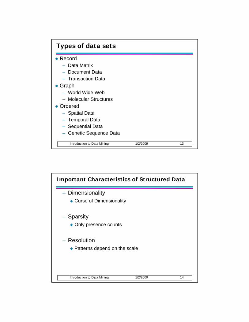
Types of data sets

Record– Data Matrix– Document Data– Transaction Data

Graph– World Wide Web– Molecular Structures

OrderedSpatial Data


– Spatial Data– Temporal Data– Sequential Data– Genetic Sequence Data

Important Characteristics of Structured Data

– DimensionalityCurse of Dimensionality

– SparsityOnly presence counts

– Resolution


Patterns depend on the scale

Record Data

Data that consists of a collection of records, each of which consists of a fixed set of attributes

Tid R f d M it l T blTid Refund MaritalStatus

TaxableIncome Cheat

1 Yes Single 125K No

2 No Married 100K No

3 No Single 70K No

4 Yes Married 120K No

5 No Divorced 95K Yes


6 No Married 60K No

7 Yes Divorced 220K No

8 No Single 85K Yes

9 No Married 75K No

10 No Single 90K Yes 10

Data Matrix

If data objects have the same fixed set of numeric attributes, then the data objects can be thought of as points in a multi-dimensional space, where each dimension represents a distinct attribute

Such data set can be represented by an m by n matrix, where there are m rows, one for each object, and n columns, one for each attribute

ThicknessLoadDistanceProjectionProjection ThicknessLoadDistanceProjectionProjection


1.12.216.226.2512.65

1.22.715.225.2710.23

Thickness LoadDistanceProjection of y load

Projection of x Load

1.12.216.226.2512.65

1.22.715.225.2710.23

Thickness LoadDistanceProjection of y load

Projection of x Load

Document Data

Each document becomes a `term' vector, – each term is a component (attribute) of the vector,

th l f h t i th b f ti– the value of each component is the number of times the corresponding term occurs in the document.


Transaction Data

A special type of record data, where – each record (transaction) involves a set of items.

F l id t Th t f– For example, consider a grocery store. The set of products purchased by a customer during one shopping trip constitute a transaction, while the individual products that were purchased are the items.

TID Items

1 Bread, Coke, Milk


2 Beer, Bread

3 Beer, Coke, Diaper, Milk

4 Beer, Bread, Diaper, Milk

5 Coke, Diaper, Milk

Graph Data

Examples: Generic graph, a Moleule, and Webpages

2

5

2

1 2

5


Benzene Molecule: C6H6

Ordered Data

Sequences of transactions

Items/Events


An element of the sequence

Ordered Data

Genomic sequence data

GGTTCCGCCTTCAGCCCCGCGCCGGTTCCGCCTTCAGCCCCGCGCCCGCAGGGCCCGCCCCGCGCCGTCGAGAAGGGCCCGCCTGGCGGGCGGGGGGAGGCGGGGCCGCCCGAGCCCAACCGAGTCCGACCAGGTGCCCCCTCTGCTCGGCCTAGACCTGA


GCTCATTAGGCGGCAGCGGACAGGCCAAGTAGAACACGCGAAGCGCTGGGCTGCCTGCTGCGACCAGGG

Ordered Data

Spatio-Temporal Data

Average Monthly Temperature of land and ocean


Data Quality

Poor data quality negatively affects many data processing efforts

“The most important point is that poor data quality is an unfoldingThe most important point is that poor data quality is an unfolding disaster.– Poor data quality costs the typical company at least ten

percent (10%) of revenue; twenty percent (20%) is probably a better estimate.”

Thomas C. Redman, DM Review, August 2004


Data mining example: a classification model for detecting people who are loan risks is built using poor data

– Some credit-worthy candidates are denied loans– More loans are given to individuals that default

Data Quality …

What kinds of data quality problems?How can we detect problems with the data? What can we do about these problems?

Examples of data quality problems: – Noise and outliers

Mi i l


– Missing values – Duplicate data

Noise

Noise refers to modification of original values– Examples: distortion of a person’s voice when talking

on a poor phone and “snow” on television screenon a poor phone and snow on television screen

Introduction to Data Mining 1/2/2009 25Two Sine Waves Two Sine Waves + Noise

Outliers are data objects with characteristics that are considerably different than most of the other data objects in the data set

Outliers

data objects in the data set– Case 1: Outliers are

noise that interfereswith data analysis

– Case 2: Outliers are th l f l i


the goal of our analysisCredit card fraudIntrusion detection

Missing Values

Reasons for missing values– Information is not collected

(e.g., people decline to give their age and weight)( g , p p g g g )– Attributes may not be applicable to all cases

(e.g., annual income is not applicable to children)

Handling missing values– Eliminate data objects

Estimate missing values


– Estimate missing valuesExample: time series of temperatureExample: census results

– Ignore the missing value during analysis

Duplicate Data

Data set may include data objects that are duplicates, or almost duplicates of one another

Major issue when merging data from heterogeous– Major issue when merging data from heterogeous sources

Examples:– Same person with multiple email addresses


Data cleaning– Process of dealing with duplicate data issues

Data Preprocessing

Aggregation

Sampling

Dimensionality Reduction

Feature subset selection

Feature creation

Discretization and Binarization


Discretization and Binarization

Attribute Transformation

Aggregation

Combining two or more attributes (or objects) into a single attribute (or object)

Purpose– Data reduction

Reduce the number of attributes or objects– Change of scale

Citi t d i t i t t t i t


Cities aggregated into regions, states, countries, etc– More “stable” data

Aggregated data tends to have less variability

Example: Precipitation in Australia

This example is based on precipitation in Australia from the period 1982 to 1993. The next slide showsThe next slide shows – A histogram for the standard deviation of average

monthly precipitation for 3,030 0.5◦ by 0.5◦ grid cells in Australia, and

– A histogram for the standard deviation of the average yearly precipitation for the same locations.


The average yearly precipitation has less variability than the average monthly precipitation. All precipitation measurements (and their standard deviations) are in centimeters.

Example: Precipitation in Australia …

Variation of Precipitation in Australia


Standard Deviation of Average Monthly Precipitation

Standard Deviation of Average Yearly Precipitation

Sampling

Sampling is the main technique employed for dataselection.

– It is often used for both the preliminary investigation ofp y gthe data and the final data analysis.

Statisticians sample because obtaining the entireset of data of interest is too expensive or timeconsuming.


Sampling …

The key principle for effective sampling is the following:

– Using a sample will work almost as well as using the entire data sets, if the sample is representative

– A sample is representative if it has approximately the same property (of interest) as the original set of data


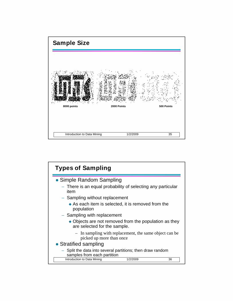
Sample Size


8000 points 2000 Points 500 Points

Types of Sampling

Simple Random Sampling– There is an equal probability of selecting any particular

item– Sampling without replacement

As each item is selected, it is removed from the population

– Sampling with replacementObjects are not removed from the population as they are selected for the sample.


– In sampling with replacement, the same object can be picked up more than once

Stratified sampling– Split the data into several partitions; then draw random

samples from each partition

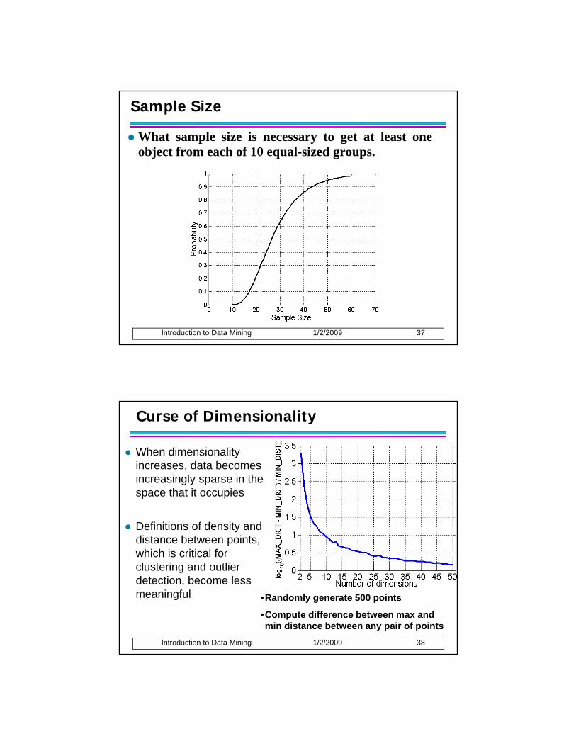
Sample Size

What sample size is necessary to get at least oneobject from each of 10 equal-sized groups.


Curse of Dimensionality

When dimensionality increases, data becomes increasingly sparse in the space that it occupies

Definitions of density and distance between points, which is critical for clustering and outlier


clustering and outlier detection, become less meaningful •Randomly generate 500 points

•Compute difference between max and min distance between any pair of points

Dimensionality Reduction

Purpose:– Avoid curse of dimensionality– Reduce amount of time and memory required by dataReduce amount of time and memory required by data

mining algorithms– Allow data to be more easily visualized– May help to eliminate irrelevant features or reduce

noise

Techniques


Techniques– Principal Components Analysis (PCA)– Singular Value Decomposition– Others: supervised and non-linear techniques

Dimensionality Reduction: PCA

Goal is to find a projection that captures the largest amount of variation in data

x2

e


x1

Dimensionality Reduction: PCA


Feature Subset Selection

Another way to reduce dimensionality of dataRedundant features

Duplicate much or all of the information contained in– Duplicate much or all of the information contained in one or more other attributes

– Example: purchase price of a product and the amount of sales tax paid

Irrelevant features– Contain no information that is useful for the data

mining task at hand


mining task at hand– Example: students' ID is often irrelevant to the task of

predicting students' GPAMany techniques developed, especially for classification

Feature Creation

Create new attributes that can capture the important information in a data set much more efficiently than the original attributesefficiently than the original attributes

Three general methodologies:– Feature extraction

Example: extracting edges from images– Feature construction


– Feature constructionExample: dividing mass by volume to get density

– Mapping data to new spaceExample: Fourier and wavelet analysis

Mapping Data to a New Space

Fourier and wavelet transform


Two Sine Waves + Noise Frequency

Frequency

Discretization

Discretization is the process of converting a continuous attribute into an ordinal attribute

A potentially infinite number of values are mapped– A potentially infinite number of values are mapped into a small number of categories

– Discretization is commonly used in classification– Many classification algorithms work best if both

the independent and dependent variables have only a few values


y– We give an illustration of the usefulness of

discretization using the Iris data set

Iris Sample Data Set

Many of the exploratory data techniques are illustrated with the Iris Plant data set.

– Can be obtained from the UCI Machine Learning Repository http://www.ics.uci.edu/~mlearn/MLRepository.html

– From the statistician Douglas Fisher– Three flower types (classes):

SetosaVirginica Versicolour


– Four (non-class) attributesSepal width and lengthPetal width and length

Virginica. Robert H. Mohlenbrock. USDA NRCS. 1995. Northeast wetland flora: Field office guide to plant species. Northeast National Technical Center, Chester, PA. Courtesy of USDA NRCS Wetland Science Institute.

Discretization: Iris Example

Petal width low or petal length low implies Setosa.Petal width medium or petal length medium implies Versicolour.Petal width high or petal length high implies Virginica.

Discretization: Iris Example …

How can we tell what the best discretization is?– Unsupervised discretization: find breaks in the data

values50

Example:Petal Length

10

20

30

40

50

Cou

nts


– Supervised discretization: Use class labels to find breaks

0 2 4 6 80

Petal Length

Discretization Without Using Class Labels


Data consists of four groups of points and two outliers. Data is one-dimensional, but a random y component is added to reduce overlap.



Equal interval width approach used to obtain 4 values.



Equal frequency approach used to obtain 4 values.



K-means approach to obtain 4 values.

Binarization

Binarization maps a continuous or categorical attribute into one or more binary variables

Typically used for association analysis

Often convert a continuous attribute to a categorical attribute and then convert a categorical attribute to a set of binary attributes


g y– Association analysis needs asymmetric binary

attributes– Examples: eye color and height measured as

{low, medium, high}

Attribute Transformation

An attribute transform is a function that maps the entire set of values of a given attribute to a new set of replacement values such that each oldset of replacement values such that each old value can be identified with one of the new values– Simple functions: xk, log(x), ex, |x|– Normalization

Refers to various techniques to adjust to differences among attributes in terms of frequency


g q yof occurrence, mean, variance, magnitude

– In statistics, standardization refers to subtracting off the means and dividing by the standard deviation

Example: Sample Time Series of Plant Growth

Minneapolis

Net Primary Production (NPP) is a measure of plant growth used by ecosystem scientists.


Correlations between time series

Minneapolis Atlanta Sao PaoloMinneapolis 1.0000 0.7591 -0.7581 Atlanta 0.7591 1.0000 -0.5739 Sao Paolo -0.7581 -0.5739 1.0000


Seasonality Accounts for Much Correlation

Minneapolis

Normalized using monthly Z Score:Subtract off monthly mean and divide by monthly standard deviation



Minneapolis Atlanta Sao PaoloMinneapolis 1.0000 0.0492 0.0906 Atlanta 0.0492 1.0000 -0.0154 Sao Paolo 0.0906 -0.0154 1.0000


Outline of Second Lecture for Chapter 2

Basics of Similarity and Dissimilarity Measures

Distances and Their Properties

Similarities and Their Properties

Density


Density

Similarity and Dissimilarity Measures

Similarity measure– Numerical measure of how alike two data objects are.

I hi h h bj t lik– Is higher when objects are more alike.– Often falls in the range [0,1]

Dissimilarity measure– Numerical measure of how different are two data

objectsLower when objects are more alike


– Lower when objects are more alike– Minimum dissimilarity is often 0– Upper limit varies

Proximity refers to a similarity or dissimilarity

Similarity/Dissimilarity for Simple Attributes

p and q are the corresponding attribute values for two data objects.


Euclidean Distance

Euclidean Distance

∑=n

qpdist 2)(

Where n is the number of dimensions (attributes) and pk and qk are, respectively, the kth attributes (components) or data objects p and q.

∑=

−=k

kk qpdist1

)(


Standardization is necessary, if scales differ.

Euclidean Distance

2

3

p1point x y

p1 0 2

0

1

0 1 2 3 4 5 6

p2

p3 p4p1 0 2p2 2 0p3 3 1p4 5 1

p1 p2 p3 p4

Introduction to Data Mining 1/2/2009 61Distance Matrix

p1 0 2.828 3.162 5.099p2 2.828 0 1.414 3.162p3 3.162 1.414 0 2p4 5.099 3.162 2 0

Minkowski Distance

Minkowski Distance is a generalization of Euclidean Distance

1

Where r is a parameter, n is the number of dimensions (attributes) and pk and qk are, respectively, the kth attributes (components) or data objects p and q.

rn

k

rkk qpdist

1

1)||( ∑

=−=


Minkowski Distance: Examples

r = 1. City block (Manhattan, taxicab, L1 norm) distance. – A common example of this is the Hamming distance, which

is just the number of bits that are different between two bi tbinary vectors

r = 2. Euclidean distance

r → ∞. “supremum” (Lmax norm, L∞ norm) distance. – This is the maximum difference between any component of


the vectors

Do not confuse r with n, i.e., all these distances are defined for all numbers of dimensions.

Minkowski Distance

L1 p1 p2 p3 p4p1 0 4 4 6p2 4 0 2 4p3 4 2 0 2

point x yp1 0 2p2 2 0p3 3 1p4 5 1

p3 4 2 0 2p4 6 4 2 0

L2 p1 p2 p3 p4p1 0 2.828 3.162 5.099p2 2.828 0 1.414 3.162p3 3.162 1.414 0 2p4 5.099 3.162 2 0

L∞ p1 p2 p3 p4


Distance Matrix

L∞ p p p pp1 0 2 3 5p2 2 0 1 3p3 3 1 0 2p4 5 3 2 0

Mahalanobis Distance

Tqpqpqpsmahalanobi )()(),( 1 −∑−= −

Σ is the covariance matrix of the input data X

∑=

−−−

=Σn

ikikjijkj XXXX

n 1, ))((

11

Determining similarity of an unknown Sample set to a known


For red points, the Euclidean distance is 14.7, Mahalanobis distance is 6.

unknown Sample set to a known one. It takes Into account the correlations of the Data set and is scale-invariant.

Mahalanobis Distance

Covariance Matrix:

⎤⎡ 2.03.0⎥⎦

⎤⎢⎣

⎡=Σ

3.02.02.03.0

A: (0.5, 0.5)

B: (0, 1)

C: (1.5, 1.5)

B

A

C


( )

Mahal(A,B) = 5

Mahal(A,C) = 4

Common Properties of a Distance

Distances, such as the Euclidean distance, have some well known properties.

1 d( ) 0 f ll d d d( ) 0 l if1. d(p, q) ≥ 0 for all p and q and d(p, q) = 0 only if p = q. (Positive definiteness)

2. d(p, q) = d(q, p) for all p and q. (Symmetry)3. d(p, r) ≤ d(p, q) + d(q, r) for all points p, q, and r.

(Triangle Inequality)

where d(p, q) is the distance (dissimilarity) between


(p, q) ( y)points (data objects), p and q.

A distance that satisfies these properties is a metric

Common Properties of a Similarity

Similarities, also have some well known properties.

1. s(p, q) = 1 (or maximum similarity) only if p = q.

2. s(p, q) = s(q, p) for all p and q. (Symmetry)

where s(p, q) is the similarity between points (data objects), p and q.


j ) p q

Similarity Between Binary Vectors

Common situation is that objects, p and q, have only binary attributes

Compute similarities using the following quantitiesg gF01 = the number of attributes where p was 0 and q was 1F10 = the number of attributes where p was 1 and q was 0F00 = the number of attributes where p was 0 and q was 0F11 = the number of attributes where p was 1 and q was 1

Simple Matching and Jaccard Coefficients S C f / f


SMC = number of matches / number of attributes = (F11 + F00) / (F01 + F10 + F11 + F00)

J = number of 11 matches / number of non-zero attributes= (F11) / (F01 + F10 + F11)

SMC versus Jaccard: Example

p = 1 0 0 0 0 0 0 0 0 0 q = 0 0 0 0 0 0 1 0 0 1

F01 = 2 (the number of attributes where p was 0 and q was 1)F01 = 1 (the number of attributes where p was 1 and q was 0)F00 = 7 (the number of attributes where p was 0 and q was 0)F11 = 0 (the number of attributes where p was 1 and q was 1)


SMC = (F11 + F00) / (F01 + F10 + F11 + F00)= (0+7) / (2+1+0+7) = 0.7

J = (F11) / (F01 + F10 + F11) = 0 / (2 + 1 + 0) = 0

Cosine Similarity

If d1 and d2 are two document vectors, thencos( d1, d2 ) = (d1 • d2) / ||d1|| ||d2|| ,

where • indicates vector dot product and || d || is thewhere indicates vector dot product and || d || is thelength of vector d.

Example:

d1 = 3 2 0 5 0 0 0 2 0 0d2 = 1 0 0 0 0 0 0 1 0 2

d • d = 3*1 + 2*0 + 0*0 + 5*0 + 0*0 + 0*0 + 0*0 + 2*1 + 0*0 + 0*2 = 5


d1 • d2= 3 1 + 2 0 + 0 0 + 5 0 + 0 0 + 0 0 + 0 0 + 2 1 + 0 0 + 0 2 = 5||d1|| = (3*3+2*2+0*0+5*5+0*0+0*0+0*0+2*2+0*0+0*0)0.5 = (42) 0.5 = 6.481||d2|| = (1*1+0*0+0*0+0*0+0*0+0*0+0*0+1*1+0*0+2*2) 0.5 = (6) 0.5 = 2.245

cos( d1, d2 ) = .3150

Extended Jaccard Coefficient (Tanimoto)

Variation of Jaccard for continuous or count attributes

Reduces to Jaccard for binary attributes– Reduces to Jaccard for binary attributes


Correlation

Correlation measures the linear relationship between objectsT t l ti t d di d tTo compute correlation, we standardize data objects, p and q, and then take their dot product

)(/))(( pstdpmeanpp kk −=′

)(/))(( td′


)(/))(( qstdqmeanqq kk −=′

)1/(),( −′•′= nqpqpncorrelatio

Visually Evaluating Correlation

Scatter plots showing the similarity from –1 to 1.

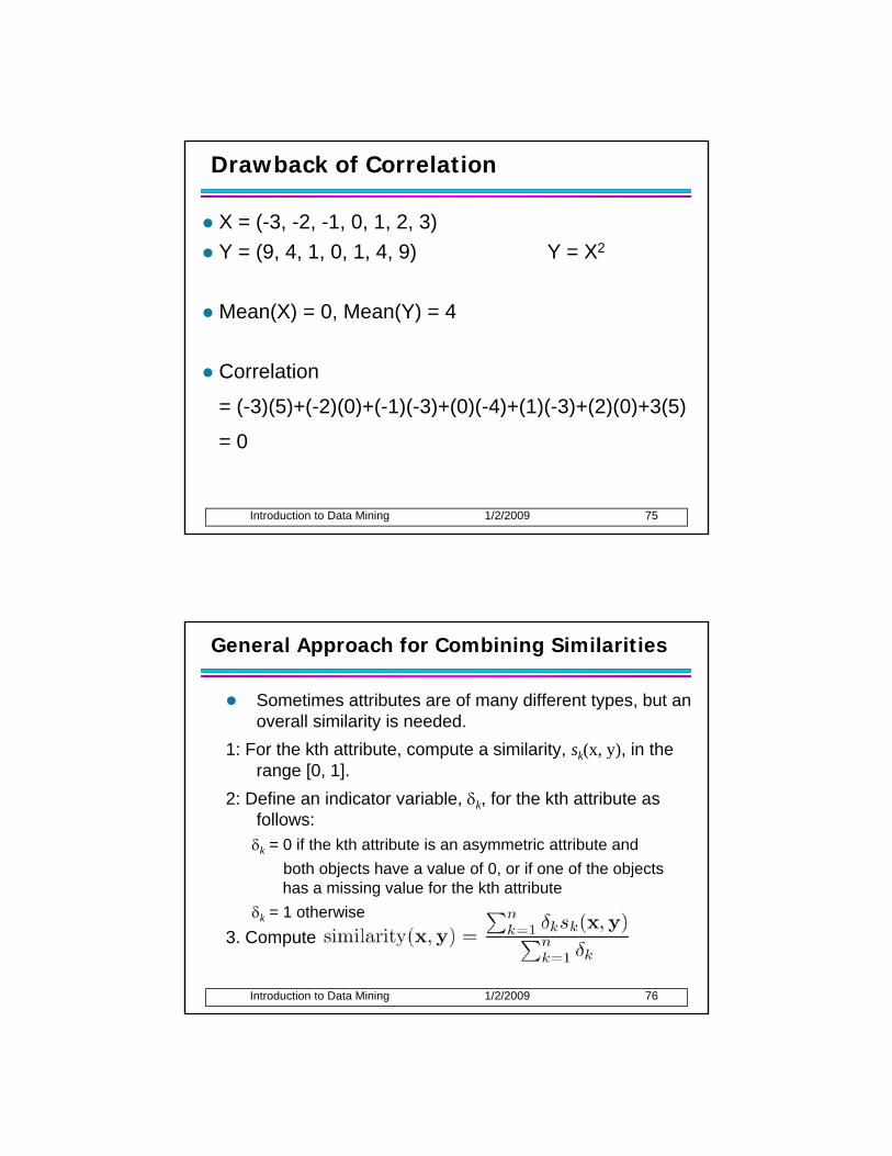
Drawback of Correlation

X = (-3, -2, -1, 0, 1, 2, 3)Y = (9, 4, 1, 0, 1, 4, 9) Y = X2

Mean(X) = 0, Mean(Y) = 4

Correlation

= ( 3)(5)+( 2)(0)+( 1)( 3)+(0)( 4)+(1)( 3)+(2)(0)+3(5)


= (-3)(5)+(-2)(0)+(-1)(-3)+(0)(-4)+(1)(-3)+(2)(0)+3(5)

= 0

General Approach for Combining Similarities

Sometimes attributes are of many different types, but an overall similarity is needed.

1: For the kth attribute compute a similarity sk(x y) in the1: For the kth attribute, compute a similarity, sk(x, y), in the range [0, 1].

2: Define an indicator variable, δk, for the kth attribute as follows:δk = 0 if the kth attribute is an asymmetric attribute and

both objects have a value of 0, or if one of the objects h i i l f th kth tt ib t


has a missing value for the kth attributeδk = 1 otherwise

3. Compute

Using Weights to Combine Similarities

May not want to treat all attributes the same.– Use weights wk which are between 0 and 1 and sum

to 1to 1.


Density

Measures the degree to which data objects are close to each other in a specified areaThe notion of density is closely related to that of proximityThe notion of density is closely related to that of proximityConcept of density is typically used for clustering and anomaly detectionExamples:– Euclidean density

Euclidean density = number of points per unit volume


– Probability densityEstimate what the distribution of the data looks like

– Graph-based densityConnectivity

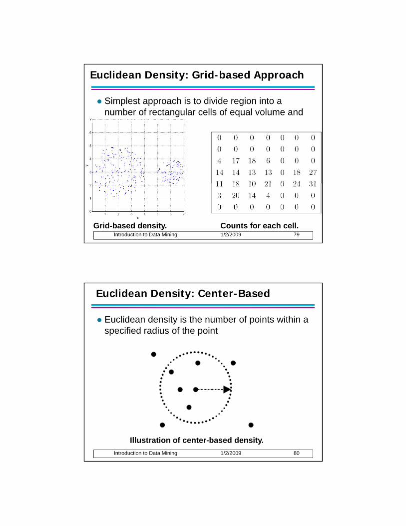
Euclidean Density: Grid-based Approach

Simplest approach is to divide region into a number of rectangular cells of equal volume and define density as # of points the cell containsdefine density as # of points the cell contains

Introduction to Data Mining 1/2/2009 79Grid-based density. Counts for each cell.

Euclidean Density: Center-Based

Euclidean density is the number of points within a specified radius of the point


Illustration of center-based density.

Data Mining: Datadatamining.rutgers.edu/teaching/fall2014/DM/lecture2.pdf · Data Mining: Data Dr....

Documents

Transcript of Data Mining: Datadatamining.rutgers.edu/teaching/fall2014/DM/lecture2.pdf · Data Mining: Data Dr....