
Data Mining I - uni-mannheim.de · University ofMannheim –Bizer: Data Mining I –FSS2019...
76
University of Mannheim – Bizer: Data Mining I – FSS2019 (Version: 14.2.2019) – Slide 1 Data Mining I Cluster Analysis
Transcript of Data Mining I - uni-mannheim.de · University ofMannheim –Bizer: Data Mining I –FSS2019...
University of Mannheim – Bizer: Data Mining I – FSS2019 (Version: 14.2.2019) – Slide 1
Data Mining I
Cluster Analysis

University of Mannheim – Bizer: Data Mining I – FSS2019 (Version: 14.2.2019) – Slide 2
Outline
1. What is Cluster Analysis?
2. K-Means Clustering
3. Density-based Clustering
4. Hierarchical Clustering
5. Proximity Measures
University of Mannheim – Bizer: Data Mining I – FSS2019 (Version: 14.2.2019) – Slide 3
1. What is Cluster Analysis?
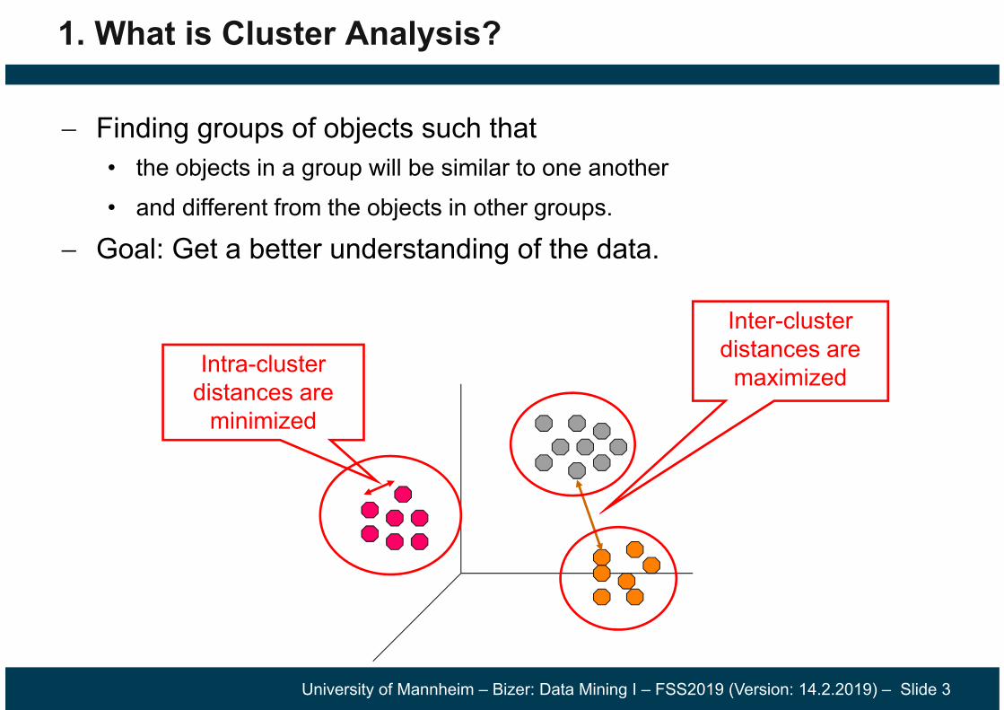
Finding groups of objects such that • the objects in a group will be similar to one another• and different from the objects in other groups.
Goal: Get a better understanding of the data.
Inter-cluster distances are
maximizedIntra-cluster distances are
minimized

University of Mannheim – Bizer: Data Mining I – FSS2019 (Version: 14.2.2019) – Slide 4
Types of Clusterings
p4p1
p3
p2
p4p1 p2 p3
Partitional Clustering• A division data objects into non-overlapping subsets (clusters) such
that each data object is in exactly one subset
Hierarchical Clustering• A set of nested clusters organized as a hierarchical tree
Dendrogram
Clustering

University of Mannheim – Bizer: Data Mining I – FSS2019 (Version: 14.2.2019) – Slide 5
Aspects of Cluster Analysis
A clustering algorithm• Partitional algorithms• Density-based algorithms• Hierarchical algorithms• …
A proximity (similarity, or dissimilarity) measure• Euclidean distance• Cosine similarity• Domain-specific similarity measures• …
Clustering Quality• Intra-clusters distance minimized.• Inter-clusters distance maximized.

University of Mannheim – Bizer: Data Mining I – FSS2019 (Version: 14.2.2019) – Slide 6
The Notion of a Cluster is Ambiguous
How many clusters?
Four Clusters Two Clusters
Six Clusters
The usefulness of a clustering depends on the goals of the analysis.

University of Mannheim – Bizer: Data Mining I – FSS2019 (Version: 14.2.2019) – Slide 7
Example Application: Market Research
Identify groups of similar customers Level of granularity depends on the task at hand Relevant customer attributes depend on the task at hand
University of Mannheim – Bizer: Data Mining I – FSS2019 (Version: 14.2.2019) – Slide 8
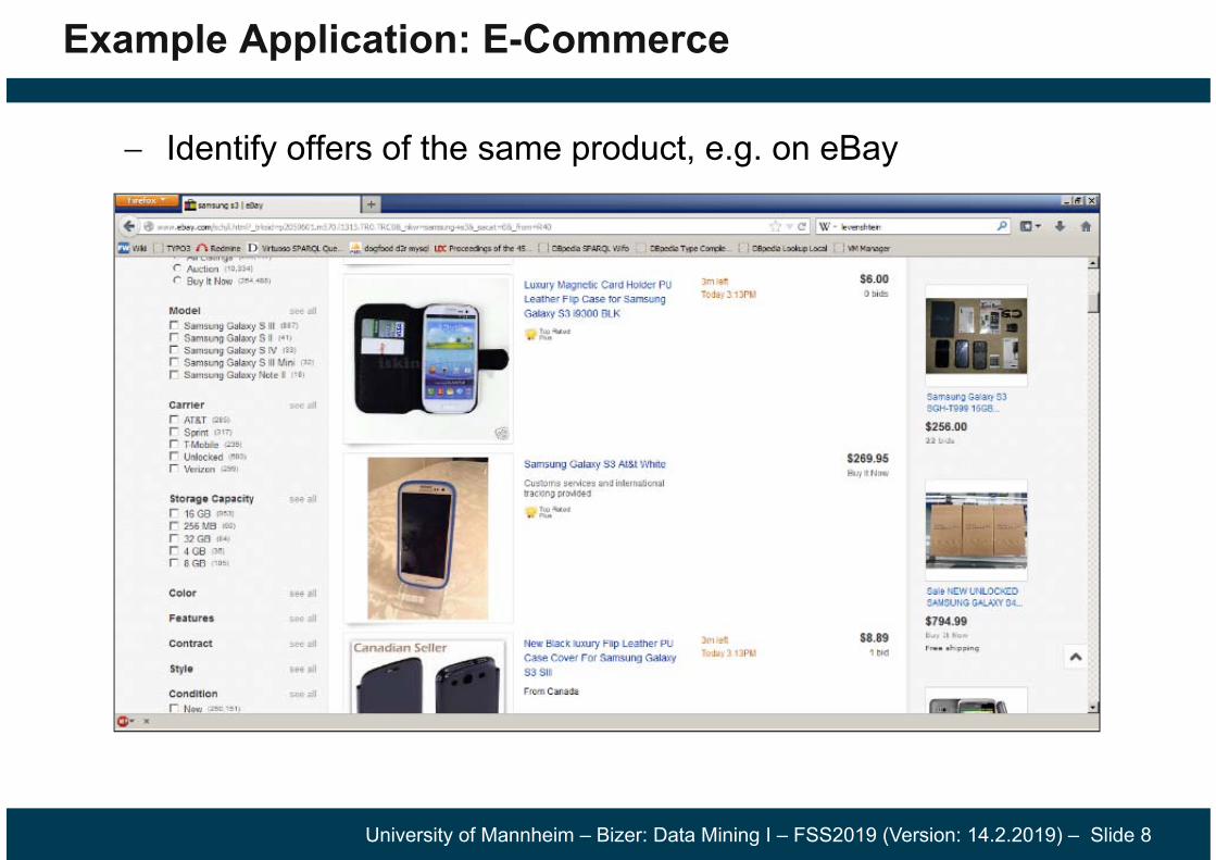
Example Application: E-Commerce
Identify offers of the same product, e.g. on eBay

University of Mannheim – Bizer: Data Mining I – FSS2019 (Version: 14.2.2019) – Slide 9
Example Application: Image Recognition
Identify parts of an image that belong to the same object
University of Mannheim – Bizer: Data Mining I – FSS2019 (Version: 14.2.2019) – Slide 10
Cluster Analysis as Unsupervised Learning
Supervised learning: Discover patterns in the data that relate data attributes with a target (class) attribute. • These patterns are then utilized to predict the values of the
target attribute in unseen data instances. • The set of classes is known before.• Training data is often provided by human annotators.
Unsupervised learning: The data has no target attribute. • We want to explore the data to find some intrinsic structures in it.• The set of classes/clusters is not known before.• No training data is used.
Cluster Analysis is an unsupervised learning task.
University of Mannheim – Bizer: Data Mining I – FSS2019 (Version: 14.2.2019) – Slide 11
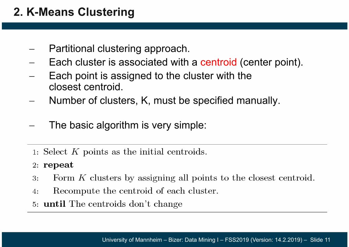
2. K-Means Clustering
Partitional clustering approach. Each cluster is associated with a centroid (center point). Each point is assigned to the cluster with the
closest centroid. Number of clusters, K, must be specified manually.
The basic algorithm is very simple:
University of Mannheim – Bizer: Data Mining I – FSS2019 (Version: 14.2.2019) – Slide 12
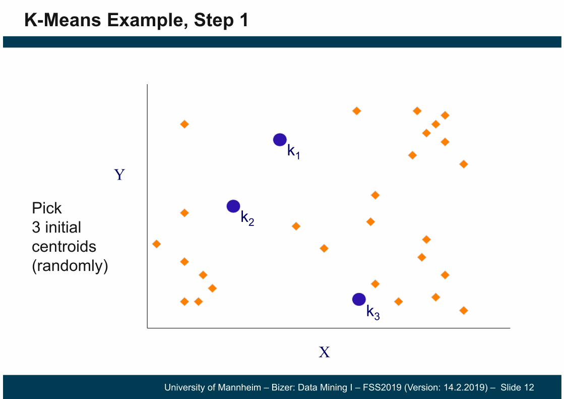
K-Means Example, Step 1
k1
k2
k3
X
Y
Pick 3 initialcentroids(randomly)
University of Mannheim – Bizer: Data Mining I – FSS2019 (Version: 14.2.2019) – Slide 13
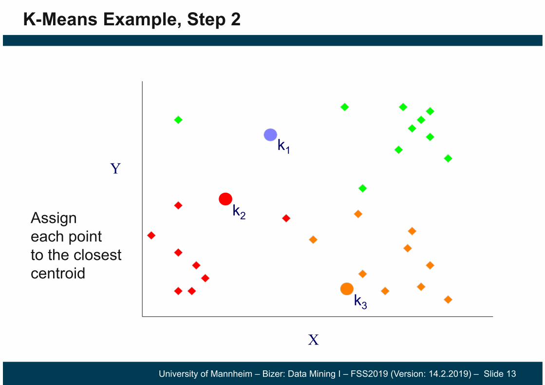
K-Means Example, Step 2
k1
k2
k3
X
Y
Assigneach pointto the closestcentroid
University of Mannheim – Bizer: Data Mining I – FSS2019 (Version: 14.2.2019) – Slide 14
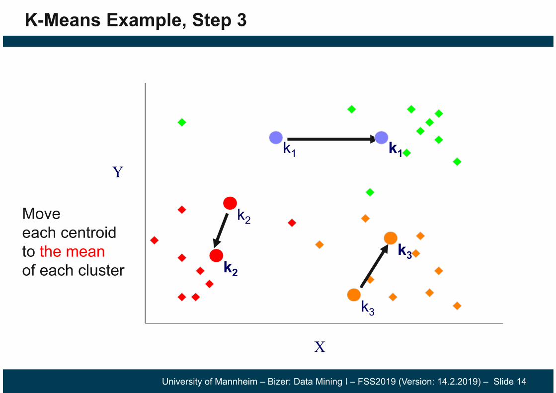
K-Means Example, Step 3
X
Y
Moveeach centroid to the meanof each cluster
k1
k2
k2
k1
k3
k3
University of Mannheim – Bizer: Data Mining I – FSS2019 (Version: 14.2.2019) – Slide 15
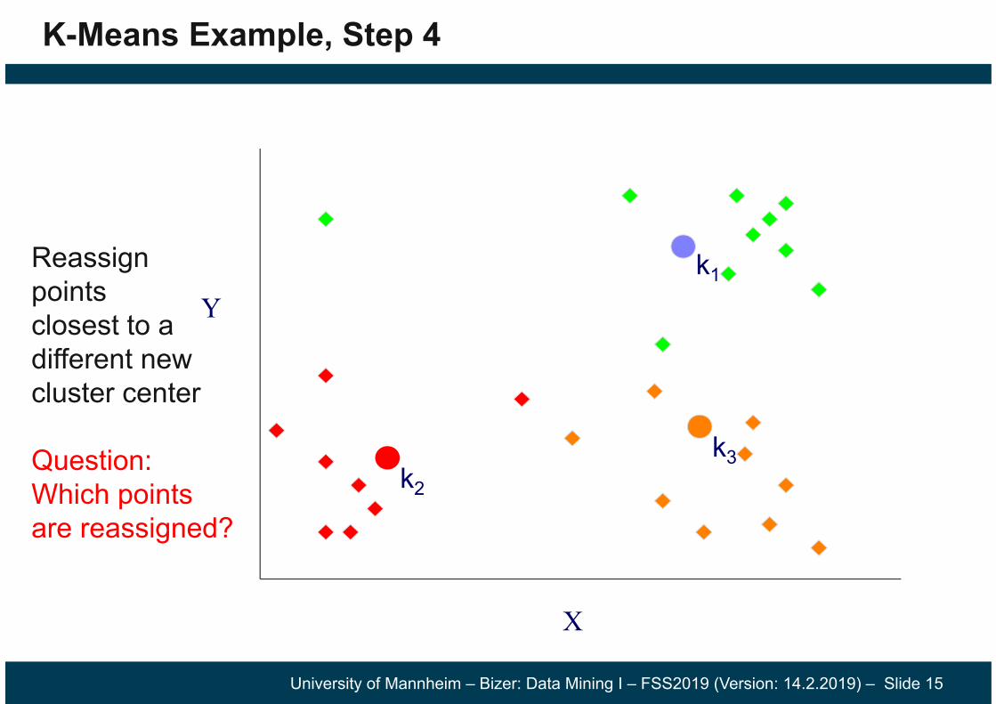
K-Means Example, Step 4
X
Y
Reassignpoints closest to a different new cluster center
Question: Which points are reassigned?
k1
k2
k3

University of Mannheim – Bizer: Data Mining I – FSS2019 (Version: 14.2.2019) – Slide 16
K-Means Example, Step 4
X
Y
Answer: Three points are reassigned
k1
k3k2

University of Mannheim – Bizer: Data Mining I – FSS2019 (Version: 14.2.2019) – Slide 17
K-Means Example, Step 5
X
Y
1. Re-compute cluster means2. Move centroids to new cluster means
k2
k3
k1

University of Mannheim – Bizer: Data Mining I – FSS2019 (Version: 14.2.2019) – Slide 18
K-Means Clustering – Second Example
-2 -1.5 -1 -0.5 0 0.5 1 1.5 2
0
0.5
1
1.5
2
2.5
3
x
y
Iteration 1
-2 -1.5 -1 -0.5 0 0.5 1 1.5 2
0
0.5
1
1.5
2
2.5
3
xy
Iteration 2
-2 -1.5 -1 -0.5 0 0.5 1 1.5 2
0
0.5
1
1.5
2
2.5
3
x
y
Iteration 3
-2 -1.5 -1 -0.5 0 0.5 1 1.5 2
0
0.5
1
1.5
2
2.5
3
x
y
Iteration 4
-2 -1.5 -1 -0.5 0 0.5 1 1.5 2
0
0.5
1
1.5
2
2.5
3
x
y
Iteration 5
-2 -1.5 -1 -0.5 0 0.5 1 1.5 2
0
0.5
1
1.5
2
2.5
3
xy
Iteration 6

University of Mannheim – Bizer: Data Mining I – FSS2019 (Version: 14.2.2019) – Slide 19
Convergence Criterions
Standard Convergence Criterion1. no (or minimum) change of centroidsAlternative Convergence Criterions1. no (or minimum) re-assignments of data points to different
clusters2. stop after X iterations3. minimum decrease in the sum of squared error (SSE)
• see next slide

University of Mannheim – Bizer: Data Mining I – FSS2019 (Version: 14.2.2019) – Slide 20
Evaluating K-Means Clusterings
Most common cohesion measure: Sum of Squared Error (SSE)• For each point, the error is the distance to the nearest centroid.• To get SSE, we square these errors and sum them.
• Cj is the j-th cluster• mj is the centroid of cluster Cj (the mean vector of all the data points in Cj), • dist(x, mj) is the distance between data point x and centroid mj.
Given several clusterings, we should prefer the one with the smallest SSE.
k
jC j
jdistSSE
1
2),(x
mx
University of Mannheim – Bizer: Data Mining I – FSS2019 (Version: 14.2.2019) – Slide 21
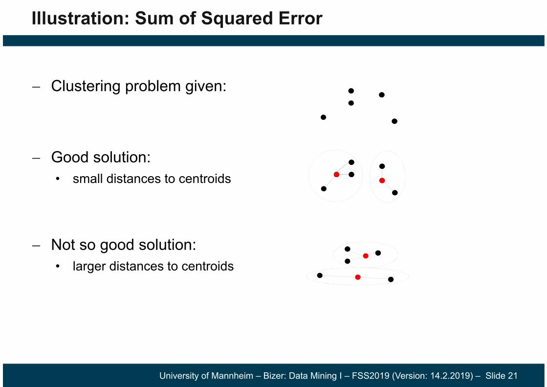
Illustration: Sum of Squared Error
Clustering problem given:
Good solution:• small distances to centroids
Not so good solution:• larger distances to centroids
University of Mannheim – Bizer: Data Mining I – FSS2019 (Version: 14.2.2019) – Slide 22
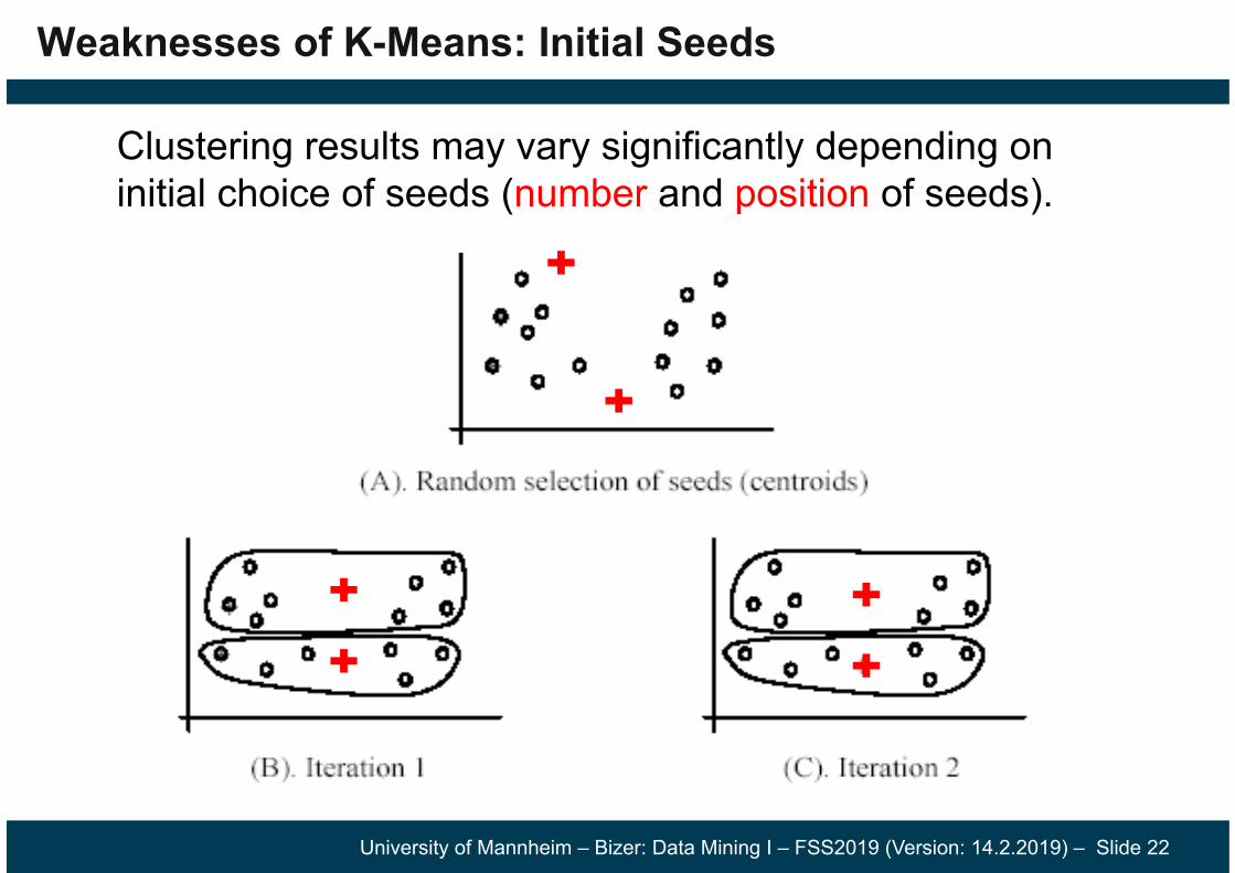
Weaknesses of K-Means: Initial Seeds
Clustering results may vary significantly depending on initial choice of seeds (number and position of seeds).

University of Mannheim – Bizer: Data Mining I – FSS2019 (Version: 14.2.2019) – Slide 23
Weaknesses of K-Means: Initial Seeds
If we use different seeds, we get good results.

University of Mannheim – Bizer: Data Mining I – FSS2019 (Version: 14.2.2019) – Slide 24
-2 -1.5 -1 -0.5 0 0.5 1 1.5 2
0
0.5
1
1.5
2
2.5
3
x
y
Iteration 1
-2 -1.5 -1 -0.5 0 0.5 1 1.5 2
0
0.5
1
1.5
2
2.5
3
x
y
Iteration 2
-2 -1.5 -1 -0.5 0 0.5 1 1.5 2
0
0.5
1
1.5
2
2.5
3
x
y
Iteration 3
-2 -1.5 -1 -0.5 0 0.5 1 1.5 2
0
0.5
1
1.5
2
2.5
3
x
y
Iteration 4
-2 -1.5 -1 -0.5 0 0.5 1 1.5 2
0
0.5
1
1.5
2
2.5
3
x
y
Iteration 5
Bad Initial Seeds – Second Example

University of Mannheim – Bizer: Data Mining I – FSS2019 (Version: 14.2.2019) – Slide 25
Weaknesses of K-Means: Initial Seeds
Approaches to increase the chance of finding good clusters:1. Restart a number of times with different random seeds
chose the resulting clustering with the smallest sum of squared error (SSE)
2. Run k-means with different values of k The SSE for different values of k cannot directly be compared.
Think: What happens for k → number of examples? Workarounds
1. Choose k where SSE improvement decreases (knee value of k)
2. Employ X-Means Variation of K-Means algorithm
that automatically determines k starts with small k, then splits large
clusters and checks if result improves
knee value

University of Mannheim – Bizer: Data Mining I – FSS2019 (Version: 14.2.2019) – Slide 26
Weaknesses of K-Means: Problems with Outliers

University of Mannheim – Bizer: Data Mining I – FSS2019 (Version: 14.2.2019) – Slide 27
Weaknesses of K-Means: Problems with Outliers
Approaches to deal with outliers:
1. K-Medoids• K-Medoids is a K-Means variation that uses the median of each
cluster instead of the mean.• Medoids are the most central existing data points in each cluster.• K-Medoids is more robust against outliers as the median is less
affected by extreme values:• Mean and Median of 1, 3, 5, 7, 9 is 5• Mean of 1, 3, 5, 7, 1009 is 205• Median of 1, 3, 5, 7, 1009 is 5
2. DBSCAN• Density-based clustering method that removes outliers.
• see next section

University of Mannheim – Bizer: Data Mining I – FSS2019 (Version: 14.2.2019) – Slide 28
K-Means Clustering Summary
Advantages
Simple, understandable
Efficient time complexity: O(t k n) where • n is the number of data points • k is the number of clusters• t is the number of iterations
Disadvantages
Need to determine number of clusters
All items are forced into a cluster
Sensitive to outliers
Sensitive to initial seeds

University of Mannheim – Bizer: Data Mining I – FSS2019 (Version: 14.2.2019) – Slide 29
K-Means Clustering in RapidMiner

University of Mannheim – Bizer: Data Mining I – FSS2019 (Version: 14.2.2019) – Slide 30
K-Means Clustering Results
New cluster attribute

University of Mannheim – Bizer: Data Mining I – FSS2019 (Version: 14.2.2019) – Slide 31
K-Medoits Clustering in RapidMiner

University of Mannheim – Bizer: Data Mining I – FSS2019 (Version: 14.2.2019) – Slide 32
X-Means Clustering in RapidMiner
Boundaries for testing k values

University of Mannheim – Bizer: Data Mining I – FSS2019 (Version: 14.2.2019) – Slide 33
3. Density-based Clustering
Challenging use case for K-Means:
Problem 1: Non-globular shapes
Problem 2: Outliers / Noise points

University of Mannheim – Bizer: Data Mining I – FSS2019 (Version: 14.2.2019) – Slide 34
DBSCAN
DBSCAN is a density-based algorithm Density = number of points within a specified radius Epsilon (Eps)
Divides data points in three classes:1. A point is a core point if it has at least a specified number of
neighboring points (MinPts) within the specified radius Eps
The point itself is counted as well
These points form the interior of a dense region (cluster)
2. A border point has fewer than MinPts within Eps, but is in the neighborhood of a core point
3. A noise point is any point that is not a core point or a border point

University of Mannheim – Bizer: Data Mining I – FSS2019 (Version: 14.2.2019) – Slide 35
Examples of Core, Border, and Noise Points 1

University of Mannheim – Bizer: Data Mining I – FSS2019 (Version: 14.2.2019) – Slide 36
Original Points Point types: core, border and noise
Examples of Core, Border, and Noise Points 2

University of Mannheim – Bizer: Data Mining I – FSS2019 (Version: 14.2.2019) – Slide 37
The DBSCAN Algorithm
Eliminates noise points and returns clustering of the remaining points:
1. Label all points as core, border, or noise points
2. Eliminate all noise points
3. Put an edge between all core points that are within Eps of each other
4. Make each group of connected core points into a separate cluster
5. Assign each border point to one of the clusters of its associated core points • as a border point can be at the border of multiple clusters• use voting if core points belong to different clusters. • if equal vote, than assign border point randomly

University of Mannheim – Bizer: Data Mining I – FSS2019 (Version: 14.2.2019) – Slide 38
How to Determine suitable Eps and MinPts values?
Eps = 9
For points in a cluster, their kth nearest neighbor (single point) should be at roughly the same distance. Noise points have their kth nearest neighbor at farther distance.1. Start with setting MinPts = 4 (rule of thumb)2. Plot sorted distance of every point to its kth nearest neighbor:
3. Set Eps to the sharp increase of the distances (start of noise points)
4. Decrease k if small clusters are labeled as noise (subjective decision)
5. Increase k if outliers are included into the clusters (subjective decision)

University of Mannheim – Bizer: Data Mining I – FSS2019 (Version: 14.2.2019) – Slide 39
When DBSCAN Works Well
Original Points Clusters
Resistant to noise
Can handle clusters of different shapes and sizes

University of Mannheim – Bizer: Data Mining I – FSS2019 (Version: 14.2.2019) – Slide 40
Application: Sky Images

University of Mannheim – Bizer: Data Mining I – FSS2019 (Version: 14.2.2019) – Slide 41
When DBSCAN Does NOT Work Well
Original Points
(MinPts=4, Eps=9.92)
(MinPts=4, Eps=9.75)
DBSCAN has problems with datasets of varying densities.
University of Mannheim – Bizer: Data Mining I – FSS2019 (Version: 14.2.2019) – Slide 42
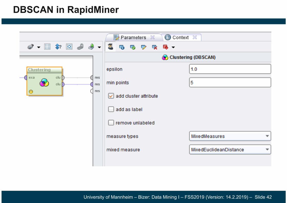
DBSCAN in RapidMiner

University of Mannheim – Bizer: Data Mining I – FSS2019 (Version: 14.2.2019) – Slide 43
4. Hierarchical Clustering
Produces a set of nested clusters organized as a hierarchical tree.
Can be visualized as a Dendrogram• A tree like diagram that records the sequences of merges or splits.• The y-axis displays the former distance between merged clusters.
1 3 2 5 4 60
0.05
0.1
0.15
0.2
1
2
3
4
5
6
1
23 4
5 Dendrogram

University of Mannheim – Bizer: Data Mining I – FSS2019 (Version: 14.2.2019) – Slide 44
Strengths of Hierarchical Clustering
We do not have to assume any particular number of clusters• any desired number of clusters can be obtained by ‘cutting’
the dendogram at the proper level.
May be used to discover meaningful taxonomies• taxonomies of biological species• taxonomies of different customer groups

University of Mannheim – Bizer: Data Mining I – FSS2019 (Version: 14.2.2019) – Slide 45
Two Main Types of Hierarchical Clustering
Agglomerative • Start with the points as individual clusters• At each step, merge the closest pair of clusters until only
one cluster (or k clusters) is left
Divisive • Start with one, all-inclusive cluster • At each step, split a cluster until each cluster contains a point
(or there are k clusters)
Agglomerative Clustering is more widely used.

University of Mannheim – Bizer: Data Mining I – FSS2019 (Version: 14.2.2019) – Slide 46
Agglomerative Clustering Algorithm
The basic algorithm is straightforward:
1. Compute the proximity matrix2. Let each data point be a cluster3. Repeat
1. Merge the two closest clusters2. Update the proximity matrixUntil only a single cluster remains
The key operation is the computation of the proximity of two clusters.
The different approaches to defining the distance between clusters distinguish the different algorithms.

University of Mannheim – Bizer: Data Mining I – FSS2019 (Version: 14.2.2019) – Slide 47
Starting Situation
Start with clusters of individual points and a proximity matrix.
p1
p3
p5p4
p2
p1 p2 p3 p4 p5 . . .
.
.
. Proximity Matrix

University of Mannheim – Bizer: Data Mining I – FSS2019 (Version: 14.2.2019) – Slide 48
Intermediate Situation
After some merging steps, we have larger clusters. We want to keep on merging the two closest clusters
(C2 and C5?)
C1
C4
C2 C5
C3

University of Mannheim – Bizer: Data Mining I – FSS2019 (Version: 14.2.2019) – Slide 49
How to Define Inter-Cluster Similarity?
Similarity?
Different Approaches possible:1. Single Link2. Complete Link 3. Group Average4. Distance Between Centroids

University of Mannheim – Bizer: Data Mining I – FSS2019 (Version: 14.2.2019) – Slide 50
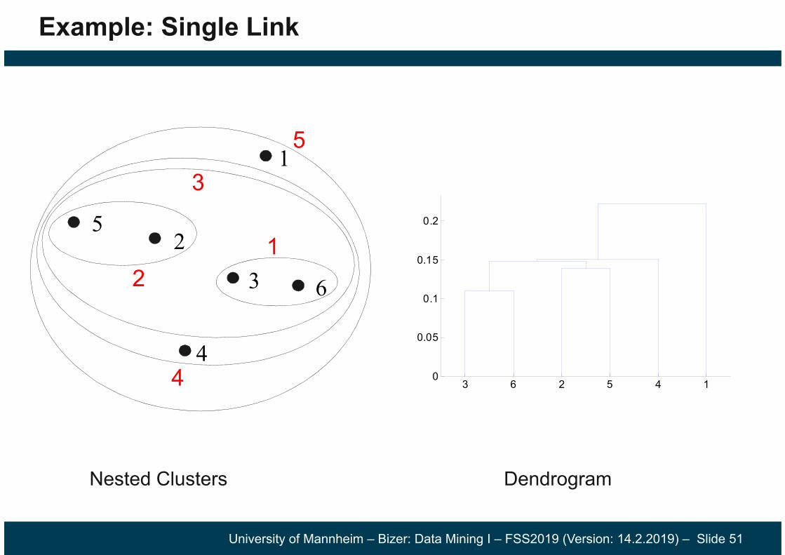
Cluster Similarity: Single Link
Similarity of two clusters is based on the two most similar (closest) points in the different clusters
Determined by one pair of points, i.e. by one link in the proximity graph.
University of Mannheim – Bizer: Data Mining I – FSS2019 (Version: 14.2.2019) – Slide 51
Example: Single Link
Nested Clusters Dendrogram
1
2
3
4
5
6
12
3
4
5
3 6 2 5 4 10
0.05
0.1
0.15
0.2

University of Mannheim – Bizer: Data Mining I – FSS2019 (Version: 14.2.2019) – Slide 52
Cluster Similarity: Complete Linkage
Similarity of two clusters is based on the two least similar (most distant) points in the different clusters
Determined by all pairs of points in the two clusters

University of Mannheim – Bizer: Data Mining I – FSS2019 (Version: 14.2.2019) – Slide 53
Example: Complete Linkage
Nested Clusters Dendrogram
3 6 4 1 2 50
0.05
0.1
0.15
0.2
0.25
0.3
0.35
0.4
1
2
3
4
5
61
2 5
3
4
University of Mannheim – Bizer: Data Mining I – FSS2019 (Version: 14.2.2019) – Slide 54
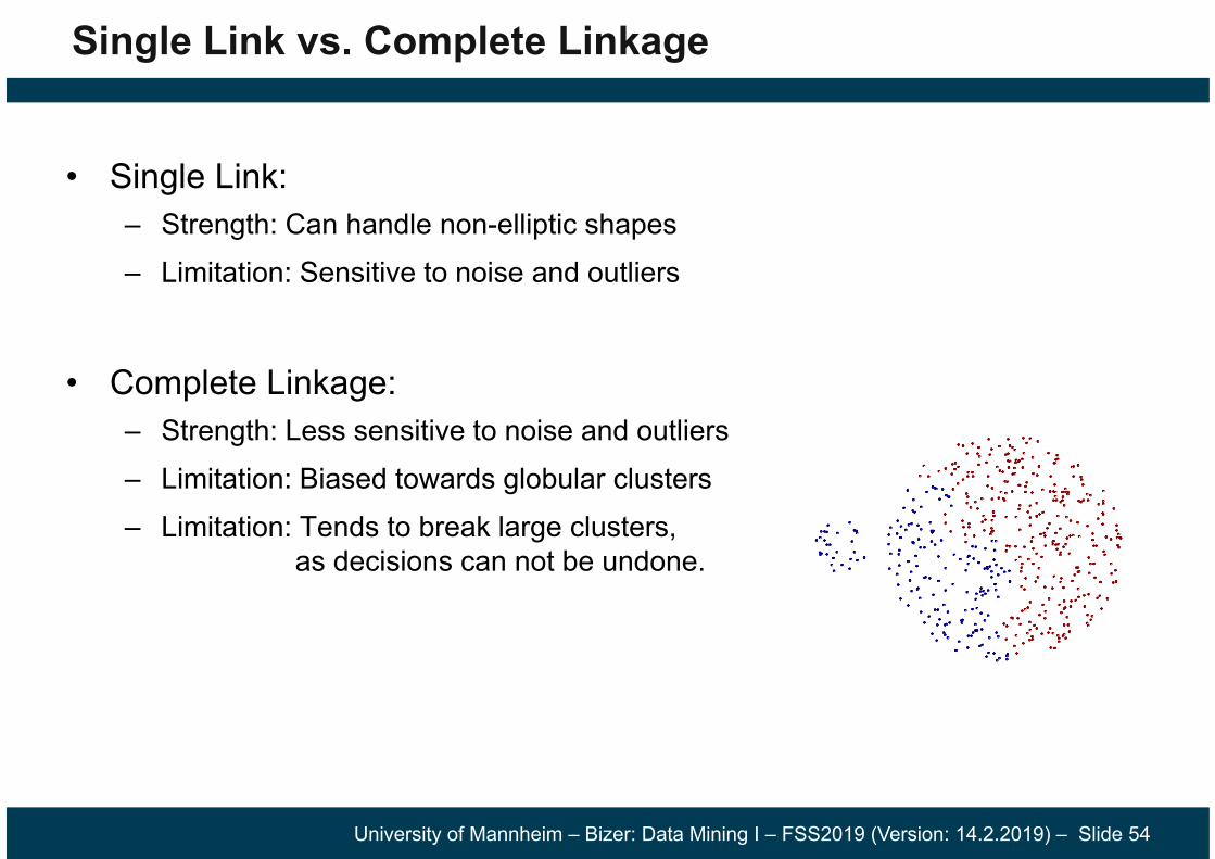
Single Link vs. Complete Linkage
• Single Link:– Strength: Can handle non-elliptic shapes– Limitation: Sensitive to noise and outliers
• Complete Linkage:– Strength: Less sensitive to noise and outliers– Limitation: Biased towards globular clusters– Limitation: Tends to break large clusters,
as decisions can not be undone.

University of Mannheim – Bizer: Data Mining I – FSS2019 (Version: 14.2.2019) – Slide 55
Cluster Similarity: Group Average
Proximity of two clusters is the average of pair-wise proximity between all points in the two clusters.
Compromise between single and complete link• Strength: Less sensitive to noise and outliers than single link• Limitation: Biased towards globular clusters
||Cluster||Cluster
)p,pproximity(
)Cluster,Clusterproximity(ji
ClusterpClusterp
ji
jijjii

University of Mannheim – Bizer: Data Mining I – FSS2019 (Version: 14.2.2019) – Slide 56
Example: Group Average
Nested Clusters Dendrogram
3 6 4 1 2 50
0.05
0.1
0.15
0.2
0.25
1
2
3
4
5
61
2
5
3
4

University of Mannheim – Bizer: Data Mining I – FSS2019 (Version: 14.2.2019) – Slide 57
Hierarchical Clustering: Problems and Limitations
Different schemes have problems with one or more of the following:1. Sensitivity to noise and outliers2. Difficulty handling non-elliptic shapes3. Breaking large clusters
High Space and Time Complexity• O(N2) space since it uses the proximity matrix.
N is the number of points.• O(N3) time in many cases
There are N steps and at each step the size N2 proximity matrix must be updated and searched.
Complexity can be reduced to O(N2 log(N)) time in some cases.• Workaround: Apply hierarchical clustering to a random sample of the
original data (<10,000 examples).

University of Mannheim – Bizer: Data Mining I – FSS2019 (Version: 14.2.2019) – Slide 58
Agglomerative Clustering in RapidMiner
Createshierarchical clustering
Flattens clustering to a given number of clusters

University of Mannheim – Bizer: Data Mining I – FSS2019 (Version: 14.2.2019) – Slide 59
5. Proximity Measures
So far, we have seen different clustering algorithms all of which rely on proximity (distance, similarity, ...) measures.
Now, we treat proximity measures in more detail.
A wide range of different measures is used depending on the requirements of the application.
Similarity• Numerical measure of how alike two data objects are.• Often falls in the range [0,1]
Dissimilarity• Numerical measure of how different are two data objects• Minimum dissimilarity is often 0• Upper limit varies

University of Mannheim – Bizer: Data Mining I – FSS2019 (Version: 14.2.2019) – Slide 60
5.1 Proximity of Single Attributes
p and q are attribute values for two data objects

University of Mannheim – Bizer: Data Mining I – FSS2019 (Version: 14.2.2019) – Slide 61
Levenshtein Distance
Measures the dissimilarity of two strings.
Measures the minimum number of edits needed to transform one string into the other.
Allowed edit operations:1. insert a character into the string
2. delete a character from the string
3. replace one character with a different character
Examples: levensthein('Table', 'Cable') = 1 (1 Substitution)
levensthein('Table', 'able') = 1 (1 Deletion)
University of Mannheim – Bizer: Data Mining I – FSS2019 (Version: 14.2.2019) – Slide 62
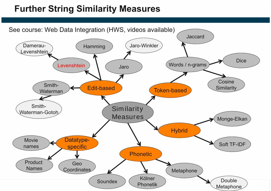
Further String Similarity Measures
SimilarityMeasures
Edit-based Token-based
Phonetic
HybridDatatype-specific
Movienames
GeoCoordinates
Soundex KölnerPhonetik
Soft TF-IDF
Monge-Elkan
Words / n-grams
Jaccard
Dice
Damerau-Levenshtein
Levenshtein Jaro
Jaro-Winkler
Smith-Waterman
Metaphone
DoubleMetaphone
Smith-Waterman-Gotoh
Hamming
CosineSimilarity
Product Names
See course: Web Data Integration (HWS, videos available)
University of Mannheim – Bizer: Data Mining I – FSS2019 (Version: 14.2.2019) – Slide 63
5.2 Proximity of Multidimensional Data Points
All measures discussed so far cover the proximity of single attribute values
But we usually have data points with many attributes
e.g., age, height, weight, sex...
Thus, we need proximity measures for data points
taking multiple attributes/dimensions into account

University of Mannheim – Bizer: Data Mining I – FSS2019 (Version: 14.2.2019) – Slide 64
Euclidean Distance
Definition
Where n is the number of dimensions (attributes) and pk and qk are the kth attributes of data points p and q.
n
kkk qpdist
1
2)(

University of Mannheim – Bizer: Data Mining I – FSS2019 (Version: 14.2.2019) – Slide 65
Example: Euclidean Distance
0
1
2
3
0 1 2 3 4 5 6
p1
p2
p3 p4
point x yp1 0 2p2 2 0p3 3 1p4 5 1
Distance Matrix
p1 p2 p3 p4p1 0 2.828 3.162 5.099p2 2.828 0 1.414 3.162p3 3.162 1.414 0 2p4 5.099 3.162 2 0

University of Mannheim – Bizer: Data Mining I – FSS2019 (Version: 14.2.2019) – Slide 66
Normalization
Attributes should be normalized so that all attributes can have equal impact on the computation of distances.
Consider the following pair of data points • xi: (0.1, 20) and xj: (0.9, 720).
The distance is almost completely dominated by (720-20) = 700.
Solution: Normalize attributes to all have a common value range, for instance [0,1].
700.000457)20720()1.09.0(),( 22 jidist xx

University of Mannheim – Bizer: Data Mining I – FSS2019 (Version: 14.2.2019) – Slide 67
Normalizing Attribute Values in Rapidminer

University of Mannheim – Bizer: Data Mining I – FSS2019 (Version: 14.2.2019) – Slide 68
Similarity of Binary Attributes
Common situation is that objects, p and q, have only binary attributes.
• Products in shopping basket• Courses attended by students
We compute similarities using the following quantities:M11 = the number of attributes where p was 1 and q was 1M00 = the number of attributes where p was 0 and q was 0M01 = the number of attributes where p was 0 and q was 1M10 = the number of attributes where p was 1 and q was 0

University of Mannheim – Bizer: Data Mining I – FSS2019 (Version: 14.2.2019) – Slide 69
Symmetric Binary Attributes
A binary attribute is symmetric if both of its states (0 and 1) have equal importance, and carry the same weights, e.g., male and female
Similarity measure: Simple Matching Coefficient
Number of matches / number of all attributes values
00111001
0011),(MMMM
MMSMC ji
xx

University of Mannheim – Bizer: Data Mining I – FSS2019 (Version: 14.2.2019) – Slide 70
Asymmetric Binary Attributes
Asymmetric: If one of the states is more important than the other. • By convention, state 1 represents the more important state.• 1 is typically the rare or infrequent state. • Examples: Shopping basket, word vector
Similarity measure: Jaccard Coefficient
Number of 11 matches / number of not-both-zero attributes values
111001
11),(MMM
MJ ji xx

University of Mannheim – Bizer: Data Mining I – FSS2019 (Version: 14.2.2019) – Slide 71
SMC versus Jaccard: Example
p = 1 0 0 0 0 0 0 0 0 0 q = 0 0 0 0 0 0 1 0 0 1
M11 = 0 (the number of attributes where p was 1 and q was 1)M00 = 7 (the number of attributes where p was 0 and q was 0)M01 = 2 (the number of attributes where p was 0 and q was 1)M10 = 1 (the number of attributes where p was 1 and q was 0)
SMC = (M11 + M00)/(M01 + M10 + M11 + M00) = (0+7) / (2+1+0+7) = 0.7
J = (M11) / (M01 + M10 + M11) = 0 / (2 + 1 + 0) = 0
University of Mannheim – Bizer: Data Mining I – FSS2019 (Version: 14.2.2019) – Slide 72
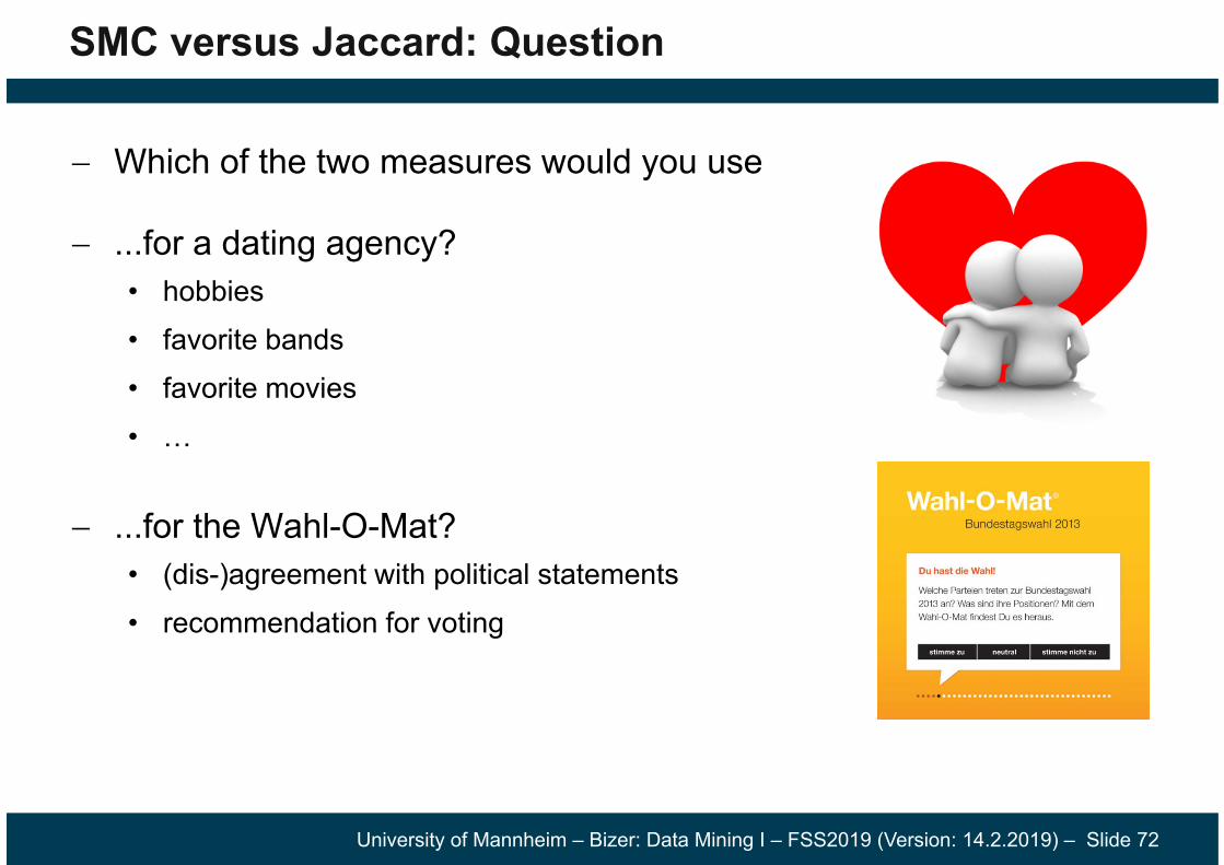
SMC versus Jaccard: Question
Which of the two measures would you use
...for a dating agency?• hobbies• favorite bands• favorite movies• …
...for the Wahl-O-Mat?• (dis-)agreement with political statements• recommendation for voting

University of Mannheim – Bizer: Data Mining I – FSS2019 (Version: 14.2.2019) – Slide 73
Using Weights to Combine Similarities
You may not want to treat all attributes the same.• Use weights wk which are between 0 and 1 and sum up to 1.• Weights are set according to the importance of the attributes.
Example: Weighted Euclidean Distance
22222
2111 )(...)()(),( jrirrjijiji xxwxxwxxwdist xx

University of Mannheim – Bizer: Data Mining I – FSS2019 (Version: 14.2.2019) – Slide 74
Combining different Similarity Measures

University of Mannheim – Bizer: Data Mining I – FSS2019 (Version: 14.2.2019) – Slide 75
How to choose a good Clustering Algorithm?
“Best” algorithm depends on1. the analytical goals of the specific use case2. the distribution of the data
Standardization of data, feature selection, distance function, and parameter settings have equally high influence on results.
Due to these complexities, the common practice is to 1. run several algorithms using different distance functions,
feature subsets and parameter settings, and 2. then visualize and interpret the results based on knowledge
about the application domain as well as the goals of the analysis.

University of Mannheim – Bizer: Data Mining I – FSS2019 (Version: 14.2.2019) – Slide 76
Literature Reference for this Slideset
Pang-Ning Tan, Michael Steinbach, Vipin Kumar: Introduction to Data Mining. Pearson / Addison Wesley.
Chapter 8: Cluster Analysis
Chapter 8.2: K-Means
Chapter 8.3: Agglomerative Hierarchical Clustering
Chapter 8.4: DBSCAN
Chapter 2.4: Measures of Similarity and Dissimilarity


![NG-DBSCAN: Scalable Density-Based Clustering for Arbitrary ...DBCURE-MR [16] is a density-based MapReduce algorithm which is not equivalent to DBSCAN: rather than circular "-neigh-borhoods,](https://static.fdocuments.in/doc/165x107/5f424d49448c527f8d210593/ng-dbscan-scalable-density-based-clustering-for-arbitrary-dbcure-mr-16-is.jpg)


