Data mining for evolution of association rules for...

Data mining for evolution of association rules for droughts and floods

in India using climate inputs

C. T. Dhanya1 and D. Nagesh Kumar1

Received 23 May 2008; revised 20 October 2008; accepted 10 November 2008; published 22 January 2009.

[1] An accurate prediction of extreme rainfall events can significantly aid in policymaking and also in designing an effective risk management system. Frequent occurrencesof droughts and floods in the past have severely affected the Indian economy, whichdepends primarily on agriculture. Data mining is a powerful new technology which helpsin extracting hidden predictive information (future trends and behaviors) from largedatabases and thus allowing decision makers to make proactive knowledge-drivendecisions. In this study, a data-mining algorithm making use of the concepts of minimaloccurrences with constraints and time lags is used to discover association rulesbetween extreme rainfall events and climatic indices. The algorithm considers only theextreme events as the target episodes (consequents) by separating these from the normalepisodes, which are quite frequent, and finds the time-lagged relationships with theclimatic indices, which are treated as the antecedents. Association rules are generated forall the five homogenous regions of India and also for All India by making use of thedata from 1960 to 1982. The analysis of the rules shows that strong relationships existbetween the climatic indices chosen, i.e., Darwin sea level pressure, North AtlanticOscillation, Nino 3.4 and sea surface temperature values, and the extreme rainfall events.Validation of the rules using data for the period 1983–2005 clearly shows that most of therules are repeating, and for some rules, even if they are not exactly the same, thecombinations of the indices mentioned in these rules are the same during validationperiod, with slight variations in the classes taken by the indices.

Citation: Dhanya, C. T., and D. Nagesh Kumar (2009), Data mining for evolution of association rules for droughts and floods in

India using climate inputs, J. Geophys. Res., 114, D02102, doi:10.1029/2008JD010485.

1. Introduction

[2] Asian monsoon greatly influences most of the tropicsand subtropics of the eastern hemisphere and more than60% of the earth’s population [Webster et al., 1998]. Whilethe failure of the monsoon brings famine, an excess orstrong monsoon will result in devastating floods, particu-larly if they are unanticipated. An accurate prediction ofthese two extremes (drought and flood) can help decisionmakers to improve planning to mitigate the adverse impactsof monsoon variability and to take advantage of beneficialconditions [Webster et al., 1998]. From the early 1900s,various climatic and oceanic parameters had been used aspredictors for monsoon rainfall prediction. Thus, if theassociation of the extremes with the climatic and oceanicparameters can be revealed, this can be used for designingan effective risk management system for facing the extremes.[3] India receives major portion of its annual rainfall

during the south west monsoon season (June–September).Even a small variation in this seasonal rainfall can have an

adverse impact on Indian economy. As per the IndianMeteorological Department (IMD), an annual rainfall eventis considered a drought (flood) if it is less (greater) than onestandard deviation from the long-term average annualrainfall. According to this definition, in the past 50 years,India has experienced around 10 droughts and 9 floods withhighest intensity of drought and flood in 1972 and 1959respectively. Two multiyear droughts also occurred in the1960s and 1980s. The frequency and intensity of drought ismuch more than of the flood.[4] Recent studies in the variation of the Gross Domestic

Product (GDP) and the monsoon [Gadgil and Gadgil, 2006]have showed that the impact of severe droughts is about 2 to5% of the GDP throughout. This indicates the need fortaking proactive steps to address the impacts of both therainfall extremes which in turn demand for an accurateprediction of the occurrence and nonoccurrence of theextremes. It is also shown that the impact of deficit rainfall(drought) on GDP is larger than that of surplus rainfall(flood).[5] Studies on the prediction of Indian Summer Monsoon

Rainfall (ISMR) have used various empirical and physical(atmospheric and coupled) models. A brief history of thesestudies and the models and predictors used is shown inTable 1. A comparative study between empirical andphysical models [Goddard et al., 2001] has shown that

JOURNAL OF GEOPHYSICAL RESEARCH, VOL. 114, D02102, doi:10.1029/2008JD010485, 2009ClickHere

for

FullArticle

1Department of Civil Engineering, Indian Institute of Science,Bangalore, India.

Copyright 2009 by the American Geophysical Union.0148-0227/09/2008JD010485$09.00

D02102 1 of 15

http://dx.doi.org/10.1029/2008JD010485

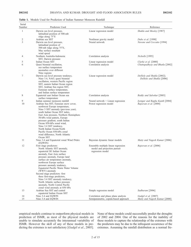
empirical models continue to outperform physical models inprediction of ISMR, as most of the physical models areunable to simulate accurately the interannual variability ofISMR. However the skill of any of these models in pre-dicting the extremes is not satisfactory [Gadgil et al., 2005].

None of these models could successfully predict the droughtsof 2002 and 2004. One of the reasons for the inability ofthese models to capture the relationship of the extremes withthe predictors may be due to the infrequent occurrence of theextremes. Assuming the rainfall distribution as a normal fre-

Table 1. Models Used for Prediction of Indian Summer Monsoon Rainfall

SerialNumber Predictors Used Technique Reference

1 Darwin sea level pressure,latitudinal position of 500-mbridge along 75�E

Linear regression model Shukla and Mooley [1987]

2 Arabian sea SST Nonlinear gravity model Dube et al. [1990]3 Darwin sea level pressure,

latitudinal position of500-mb ridge along 75�E,May surface resultantwind speed

Neural network Navone and Ceccatto [1994]

4 Northern Australia-IndonesiaSST, Darwin pressure

Correlation analysis Nicholls [1995]

5 Indian Ocean SST Linear regression model Clarke et al. [2000]6 Quasi biennial oscillation,

sea surface temperatureanomalies over differentNino regions

Correlation analysis Chattopadhyay and Bhatla [2002]

7 Darwin sea level pressure tendency,Nino 3.4, NAO, quasi biennialoscillation, western Pacific regionSST, eastern Indian Ocean regionSST, Arabian Sea region SST,Eurasian surface temperature,and Indian surface temperature

Linear regression model DelSole and Shukla [2002];DelSole and Shukla [2006]

8 Equatorial east Indian Ocean seasurface temperature

Correlation analysis Reddy and Salvekar [2003]

9 Indian summer monsoon rainfall Neural network + Linear regression Iyengar and Raghu Kanth [2004]10 Arabian Sea SST, Eurasian snow cover,

northwest Europe temperature,Nino 3 SST anomaly (previous year),south Indian Ocean SST index,East Asia pressure, Northern Hemisphere50-hPa wind pattern, Europepressure gradient, south IndianOcean 850-hPa zonal wind,Nino 3.4 SST tendency,North Indian Ocean-NorthPacific Ocean 850-hPa zonalwind difference, North AtlanticOcean SST

Power regression model Rajeevan et al. [2004]

11 Nino 3.4 and Equatorial zonal Wind INdex(EQWIN)

Bayesian dynamic linear models Maity and Nagesh Kumar [2006]

12 First stage predictors:North Atlantic SST anomaly,equatorial SE Indian Oceananomaly, East Asia surfacepressure anomaly, Europe landsurface air temperature anomaly,northwest Europe surfacepressure anomaly tendency,Equatorial Pacific Warm Water Volume(WWV) anomaly

Ensemble multiple linear regressionmodel and projection pursuitregression model

Rajeevan et al. [2006]

Second stage predictors: firstthree first-stage predictors,Nino 3.4 SST anomaly tendency,North Atlantic surface pressureanomaly, North Central Pacificzonal wind anomaly at 850 hPa

13 Arabian Sea SST and centralequatorial Indian Ocean SST

Simple regression model Sadhuram [2006]

14 Nino 3.4 and EQWIN Correlation and phase plane analysis Gadgil et al. [2007]15 Nino 3.4 and EQWIN Semiparametric, copula-based approach Maity and Nagesh Kumar [2008]

D02102 DHANYA AND KUMAR: DROUGHT AND FLOOD ASSOCIATION RULES

2 of 15

D02102

quency curve, the occurrence of either drought or floodcovers only 16% of the time (since only 16% of the distrib-ution area is less than the mean � 1 � standard deviation).[6] In this study, a time series data-mining algorithm

is used to generate the association rules between oceanicand atmospheric parameters and rainfall extremes. In thisattempt, attention is given to find the relationship betweenonly the extremes and the predictors, without consideringthe normal rainfall which is quite frequent. By using such adata-mining algorithm in this context, one of the advantagesis that there is no need to have a prior idea about thecorrelation and causal relationships between the variables.Unlike the empirical methods, this method takes intoaccount the interrelationships between the predictor varia-bles very well. The exact values of the model parameterssuch as coefficients in a regression model or weights in aneural network are of little importance in this approach.Thus the objective here is to unearth all the frequent patterns(episodes) of the predictors that precede the extreme epi-sodes of rainfall using a time series data-mining algorithm.

2. Time Series Data Mining

[7] Data mining can be defined as a process in whichspecific algorithms are used for extracting some newnontrivial information from large databases. Data-miningtechniques are widely applied in business activities and alsoin scientific and engineering scenarios. Various data-miningtechniques can be broadly classified into two types [Hanand Kamber, 2006]: descriptive data mining, in which thedata in the database are characterized according to theirgeneral properties and predictive data mining, in whichpredictions are made by performing inference from thecurrent data. Frequent patterns and association rules, clus-tering and deviation detection come under the first categorywhile regression and classification come under the secondone. Almost all the studies done so far on rainfall extremesare based on the predictive data-mining techniques. Asmentioned earlier, these studies were unable to successfullypredict the infrequent extreme episodes. Hence, in thisstudy, a descriptive data-mining technique is used to captureespecially the infrequent extreme episodes.[8] Temporal data mining is concerned with data mining

of large sequential sets (ordered data with respect to someindex). Time series is a popular class of sequential data inwhich records are indexed by time. The possible objectivesin the case of temporal data mining can be grouped asfollows: (1) prediction, (2) classification, (3) clustering,(4) search and retrieval, and (5) pattern discovery [Hanand Kamber, 2006]. Among these, algorithms of patterninterest are of most recent origin. The word ‘‘pattern’’means a local structure in the data. The objective is tosimply unearth all patterns of interest. One common mea-sure to assess the value of a pattern is the frequency of thepattern. A frequent pattern is one that occurs many times inthe data. The frequent patterns thus discovered can be usedto discover the causal rules.[9] A rule consists of a left-hand side proposition (ante-

cedent) and a right hand side proposition (consequent). Therule states that when the antecedent occurs (is true), then theconsequent also occurs (is true). Rule based approaches are

often used to ascertain the relationships within the data set.For example, association rules determine the rules thatindicate whether or how much the values of an attributedepend on the values of the other attributes in the data set.These are used to capture correlations between differentattributes in the data. In such cases, the conditional proba-bility of the occurrence of the consequent given the ante-cedent is referred to as the confidence of the rule. Forexample, if a pattern ‘‘B follows A’’ occurs n1 times and thepattern ‘‘C follows B follows A’’ occurs n2 times, then thetemporal association rule ‘‘whenever B follows A, C willalso follow’’ has a confidence of (n2/n1). The value of a ruleis usually measured in terms of its confidence.[10] There are two popular frameworks for frequent

pattern discovery namely sequential patterns and episodes.In the sequential patterns framework, a collection of sequen-ces are given and the task is to discover the order ofsequences of the items (i.e., sequential patterns) that occursin sufficiently good number of those sequences. In thefrequent episodes framework, the data are given in a singlelong sequence and the task is to unearth temporal patterns(called episodes) that occur sufficiently often along thatsequence. Frequent episodes framework is used in thepresent study, since one does not know in prior all thesequences to be searched in the time series as is required insequential patterns framework. Also, concern is to extractthe temporal patterns of the climatic indices and extremeevents which can be done by applying frequent episodesframework. Several algorithms were formulated [Mannila etal., 1997] for the discovery of frequent episodes within onesequence.

2.1. Framework of Frequent Episode Discovery

2.1.1. Event Sequence[11] The data, referred to here as an event sequence, are

denoted by h(E1, t1), (E2, t2),. . .i where Ei takes values froma finite set of event types e, and ti is an integer denoting thetime stamp of the ith event. The sequence is ordered withrespect to the time stamps so that, ti � ti+1 for all i = 1, 2,. . ..The following is a sample event sequence with six eventtypes A, B, C, D, E and F in it:

[12] Any event sequence can be expressed as a tripleelement (s, TB, TD) where s is the time-ordered sequence ofevents from beginning to end, TB is the beginning time andTD is the ending time.The above sample event sequencecan be expressed as S = (s, 9, 43) where s = h(B, 10), (C, 11),(A, 12), (F, 13), (A, 15), . . . (C, 42)i.2.1.2. Episode[13] An episode a is defined by a triple element (Va, �a,

ga), where Va is a collection of nodes, �a is a partial orderon Va and ga: Va ! e is a map that associates each node inthe episode with an event type. Thus an episode is acombination of events with a time-specified order. Whenthere is a fixed order among the event types of an episode, itis called a serial episode and when there is no order at all,the episode is called a parallel episode.


3 of 15

D02102

[14] An episode is said to occur in an event sequence ifthere exist events in the sequence occurring in exactly thesame order as that prescribed in the episode, within a giventime bound. For example, in the above sample eventsequence, the events (A, 19), (B, 21) and (C, 22) constitutean occurrence of a 3-node serial episode (A ! B ! C)while the events (A, 12), (B, 10) and (C, 11) do not, be-cause for this serial episode to occur, A must occur beforeB and C.2.1.3. Window[15] Now, to find all frequent episodes from a class of

episodes, the user has to define how close is close enoughby defining a time window width within which the episodesshould appear. For an episode to be interesting, the events inan episode must occur close to each other in time span. Awindow can be defined as a slice of an event sequence andthen the event is considered as a sequence of partiallyoverlapping windows. A window on an event sequence (s,Ts, Te) can also be expressed as a triple element w = (w, ts,te)., where ts < Te, te > Ts and w consists of those event pairsfrom s where ts � ti � te. The time span te � ts is called thewidth of the window w.[16] Consider the example of event sequence given

above. Two windows of width 5 are shown. The firstwindow starting at time 10 is shown in solid line, followedby a second window shown in dashed line. First window canbe represented as (h(B, 10), (C, 11), (A, 12), (F, 13)i, 10, 15).Here the event (A, 15) occurred at the ending time is notincluded in the sequence. Similarly, the second window canbe represented as (h(C, 11), (A, 12), (F, 13), (A, 15)i, 11, 16).[17] For a sequence S with a given window width ‘‘win’’,

the total number of windows possible is given byW(s, win) =Te � Ts + win. This is because the first and last windowsextend outside the sequence, such that the first windowcontains only the first time stamp of the sequence and thelast window contains only the last time stamp. Hence an eventclose to either end of a sequence is observed in equally manywindows to an event in the middle of the sequence. For thesequence given above, totally there are 39 partially over-lapping windows with first window (F, 5, 10) and lastwindow (F, 43, 48).[18] The frequency of an episode is defined as the number

of windows in which the episode occurs divided by the totalnumber of windows in the data set. For the 3-node serialepisode (A ! B ! C), there are only two occurrences i.e.,in windows (h(F, 18), (A, 19), (B, 21), (C, 22), 18, 23) and(h(A, 19), (B, 21), (C, 22), (E, 23)i, 19, 24). Thus thefrequency of the episode is (2/39) � 100 = 5.13%. Now,given an event sequence, a window width and a frequencythreshold, the task is to discover all frequent episodes in theevent sequence.[19] Once the frequent episodes are known, it is possible

to generate rules that describe temporal correlations be-tween events. However, there can be other ways to defineepisode frequency.2.1.4. MINEPI Algorithm[20] One such alternative proposed by Mannila et al.

[1997] is MINEPI algorithm and is based on counting whatare known as minimal occurrences of episodes. A minimaloccurrence of an episode is defined as a window (orcontiguous slice) of the input sequence in which the episodeoccurs, subject to the condition that no proper subwindow

of this window contains an occurrence of the episode. Thealgorithm for counting minimal occurrences trades spaceefficiency for time efficiency as compared to the windows-based counting algorithm. In addition, since the algorithmlocates and directly counts occurrences (as against countingthe number of windows in which episodes occur), itfacilitates the discovery of patterns with extra constraints(such as being able to discover rules of the form ‘‘if A and Boccur within 10 seconds of one another, C follows withinanother 20 seconds’’).[21] Minimal occurrences of episodes with their time

intervals are identified in the following way. For a givenepisode a and an event sequence S, the minimal occurrenceof a in S is the interval [ts, te], if (1) a occurs in the windoww = (w, ts, te) on S, and if (2) a does not occur in any propersubwindow on w. Awindow w0 = (w0, t0s, t

0e) will be a proper

subwindow of w if ts � t0s, t0e � te, and width(w0) <width(w). The set of minimal occurrences of an episode ain a given event sequence is denoted by mo(a) = {[ts, te)j[ts,te)} . For the example sequence given above, the serialepisode a = B ! C has four minimal occurrences i.e.,mo(a) = {[10,11), [21,22), [32,36), [38,42)}.[22] The concept of frequency of episodes explained in

the previous section is not very useful in the case ofminimal occurrences as there is no fixed window size andalso a window may contain several minimal occurrences ofan episode. Therefore Mannila et al. [1997] used theconcept of support instead of frequency. The support ofan episode a in a given event sequence S is jmo(a)j. Anepisode a is frequent if jmo(a)j user defined minimumsupport threshold.2.1.5. MOWCATL Algorithm[23] The above approach was modified to handle separate

antecedent and consequent constraints and maximum win-dow widths and also the time lags between the antecedentand consequent to find natural delays embedded within theepisodal relationships by Harms and Deogun [2004] inMinimal Occurrences With Constraints And Time Lags(MOWCATL) algorithm. Although MINEPI and MOW-CATL both use the concept of minimal occurrences to findthe episodal relationships, MOWCATL has some additionalmechanisms like (1) allowing a time lag between theantecedent and consequent of a discovered rule, and (2)working with episodes from across multiple sequences[Harms et al., 2002]. Episodal rules are found out wherethe antecedent episode occurs within a given maximumwindow width wina, the consequent episode occurs within agiven maximum window width winc, and the start of theconsequent follows the start of the antecedent within a givenmaximum time lag. This algorithm allows to find rules ofthe form: ‘‘if A and B occur within 3 months, then within 2months they will be followed by C and D occurring togetherwithin 4 months’’.[24] This algorithm first goes through the data sequence

and stores the occurrences of all single events for theantecedent and consequent separately. The algorithm onlylooks for the target episodes specified by the user. So itprunes the episodes that do not meet the user specifiedminimum support threshold. Then two event episodes aregenerated by pairing up the single events so that the pairs ofevents occur within the prescribed window width and theoccurrences of these two event episodes in the data se-


4 of 15

D02102

quence are recorded. This is repeated until there are no moreevents to be paired up. The process repeats for three events,four events and so on until there are no episodes left to becombined that meet the minimum threshold. The frequentepisodes for antecedent and consequent sequences are foundindependently. These frequent episodes are combined toform an episodal rule.[25] An episodal rule is that in which an antecedent

episode occurs within a given window width, a consequentepisode occurs within a given window width and the start ofthe consequent follows the start of the antecedent within auser specified time lag. For example, let episode X is of theevents A and B, and episode Y is of the events C and D.Also the user specified antecedent window width is 3months, consequent window width is 2 months and thetime lag is 3 months. Then the rule generated would indicatethat if A and B occur within 3 months, then within 3 monthsthey will be followed by C and D occurring together within2 months. The support of the rule is the number of times therule occurs in the data sequence. The confidence of the ruleis the conditional probability that the consequent occurs,given the antecedent occurs. For the rule ‘‘X is followed byY’’, the confidence is the ratio of the Support[X and Y] andSupport[X]. Here X is a serial antecedent episode (A ! B)and Y is a serial consequent episode (C ! D).

[26] The support and confidence are the two measuresused for measuring the value of the rule. The values of theseare set high to prune the association rules. Even after settingthe threshold of these measures high, there will be anadequate number of rules, making the user’s task of ruleselection difficult. The user needs some quantifying meas-ures to select the most valuable rules in addition to thesupport and confidence measures. Several interestingness orgoodness measures are used to compare and select betterrules from the ones that are generated [Bayardo andAgarwal, 1999; Das et al., 1998; Harms et al., 2002]. InMOWCATL algorithm, J measure is used for rule ranking[Smyth and Goodman, 1991]. The J measure is given by

J x; yð Þ ¼ p xð Þp yjxð Þ � log p yjxð Þ=p yð Þ½ �þ

1� p yjxð Þ½ � � log 1� p yjxð Þ½ �= 1� p yð Þ½ �f g

24

35

ð1Þ

where p(x), p(y) and p(yjx) are the probabilities ofoccurrence of x, y and y given x respectively in the datasequence. The first term in the J measure is a bias towardrules which occur more frequently. The second term i.e., theterm inside the square brackets is well known as cross-entropy, namely the information gained in going from the

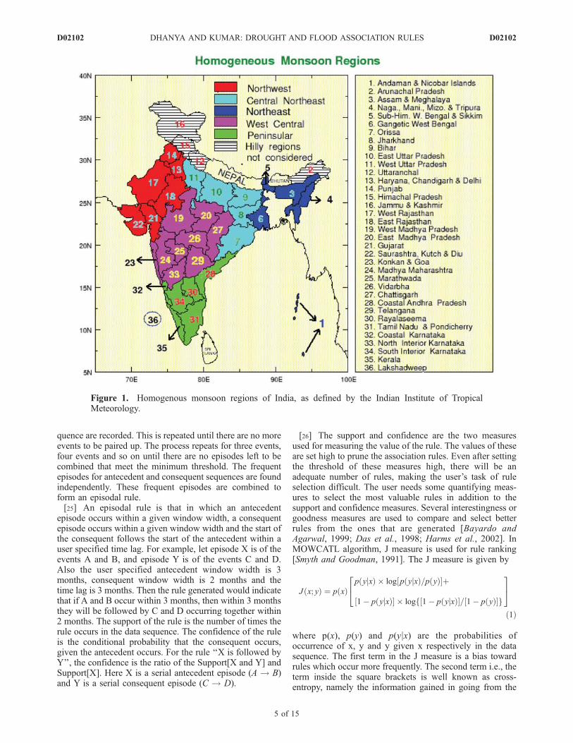
Figure 1. Homogenous monsoon regions of India, as defined by the Indian Institute of TropicalMeteorology.


5 of 15

D02102

prior probability p(y) to a posterior probability p(yjx) [Daset al., 1998]. Compared to other measures which directlydepend on the probabilities [Piatetsky-Shapiro, 1991],thereby assigning less weight to the rarer events, J measureis better suited to rarer events since it uses a log scale(information based). As shown by Smyth and Goodman[1991], J measure has the unique properties as a ruleinformation measure and is a special case of Shannon’smutual information.[27] The J values range from 0 to 1. The higher the J

value the better it is. However, since drought and flood areso infrequent, the J values are so small that all values greaterthan 0.025 are to be considered.[28] MOWCATL algorithm is used in the present study

for extracting rules between extreme episodes and climaticindices, since this algorithm can be used for multiplesequences and also this will capture by itself the lagbetween the occurrences of climatic indices and rainfallevents.

3. Data Used for the Study

[29] The time series data sets used in this study are of themonthly values for the period 1960 to 2005 and are definedas follows.

[30] 1. Summer monsoonal rainfall (June to September)for All India and also for the five homogeneous regions (asdefined by Indian Institute of Tropical Meteorology), for theperiod 1960 to 2005 (http://www.tropmet.res.in).[31] 2. Darwin sea level pressure (DSLP), (NCEP,

ftp.ncep.noaa.gov/pub/cpc/wd52dg/data/indices).[32] 3. Nino 3.4, east central tropical Pacific sea surface

temperature (SST), 170�E–120�W, 5�S–5�N (http://www.cpc.ncep.noaa.gov/data/indices/sstoi.indices).[33] 4. North Atlantic Oscillation (NAO), normalized sea

level pressure difference between Gibraltor and southwestIceland (http://www.cru.uea.ac.uk/cru/data/nao.htm).[34] 5. 1 � 1 degree grid SST data over the region 40�E–

120�E, 25�S–25�N (ICOADS, http://www.cdc.noaa.gov/icoads-las/servlets/datset).

4. Association Rules for Extremes

[35] The data-mining algorithm is applied to find theassociation rules of the extreme rainfall episodes with theclimatic indices and thus to find the spatial and temporalpatterns of extreme episodes throughout the country. Thegeographical locations of the homogenous regions: north-west, central northeast, northeast, west central and peninsu-lar are shown in Figure 1.

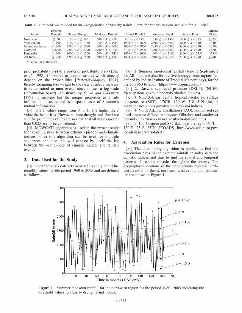
Table 2. Threshold Values Used for the Categorization of Monthly Rainfall (mm) for Various Regions and Also for All Indiaa

RegionExtremeDrought Severe Drought Moderate Drought Normal Rainfall Moderate Flood Severe Flood

ExtremeFlood

Northwest �150 150 < X � 500 500 < X � 850 850 < X < 1550 1550 � X < 1900 1900 � X < 2250 2250West central �1100 1100 < X � 1450 1450 < X � 1900 1900 < X < 2600 2600 � X < 3000 3000 � X < 3400 3400Central northeast �1200 1200 < X � 1600 1600 < X � 2000 2000 < X < 2850 2850 � X < 3300 3300 � X < 3700 3700Northeast �2200 2200 < X � 2700 2700 < X � 3100 3100 < X < 3900 3900 � X < 4300 4300 � X < 4700 4700Peninsular �1000 1000 < X � 1200 1200 < X � 1450 1450 < X < 1900 1900 � X < 2100 2100 � X < 2350 2350All India �1200 1200 < X � 1500 1500 < X � 1800 1800 < X < 2400 2400 � X < 2700 2700 � X < 2900 2900

aRainfall in millimeters.

Figure 2. Summer monsoon rainfall for the northwest region for the period 1960–2005 indicating thethreshold values to classify droughts and floods.


6 of 15

D02102

4.1. Selection of Consequent Episodes

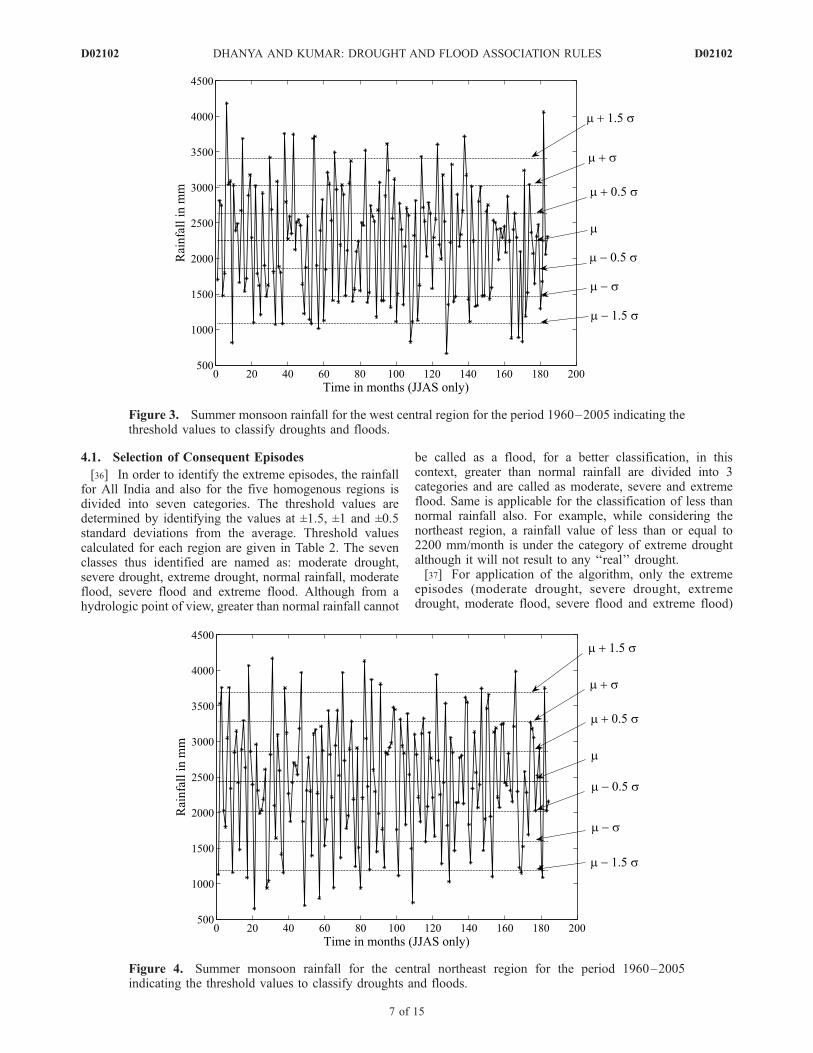
[36] In order to identify the extreme episodes, the rainfallfor All India and also for the five homogenous regions isdivided into seven categories. The threshold values aredetermined by identifying the values at ±1.5, ±1 and ±0.5standard deviations from the average. Threshold valuescalculated for each region are given in Table 2. The sevenclasses thus identified are named as: moderate drought,severe drought, extreme drought, normal rainfall, moderateflood, severe flood and extreme flood. Although from ahydrologic point of view, greater than normal rainfall cannot

be called as a flood, for a better classification, in thiscontext, greater than normal rainfall are divided into 3categories and are called as moderate, severe and extremeflood. Same is applicable for the classification of less thannormal rainfall also. For example, while considering thenortheast region, a rainfall value of less than or equal to2200 mm/month is under the category of extreme droughtalthough it will not result to any ‘‘real’’ drought.[37] For application of the algorithm, only the extreme

episodes (moderate drought, severe drought, extremedrought, moderate flood, severe flood and extreme flood)

Figure 3. Summer monsoon rainfall for the west central region for the period 1960–2005 indicating thethreshold values to classify droughts and floods.

Figure 4. Summer monsoon rainfall for the central northeast region for the period 1960–2005indicating the threshold values to classify droughts and floods.


7 of 15

D02102

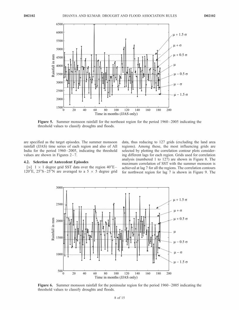
are specified as the target episodes. The summer monsoonrainfall (JJAS) time series of each region and also of AllIndia for the period 1960–2005, indicating the thresholdvalues are shown in Figures 2–7.

4.2. Selection of Antecedent Episodes

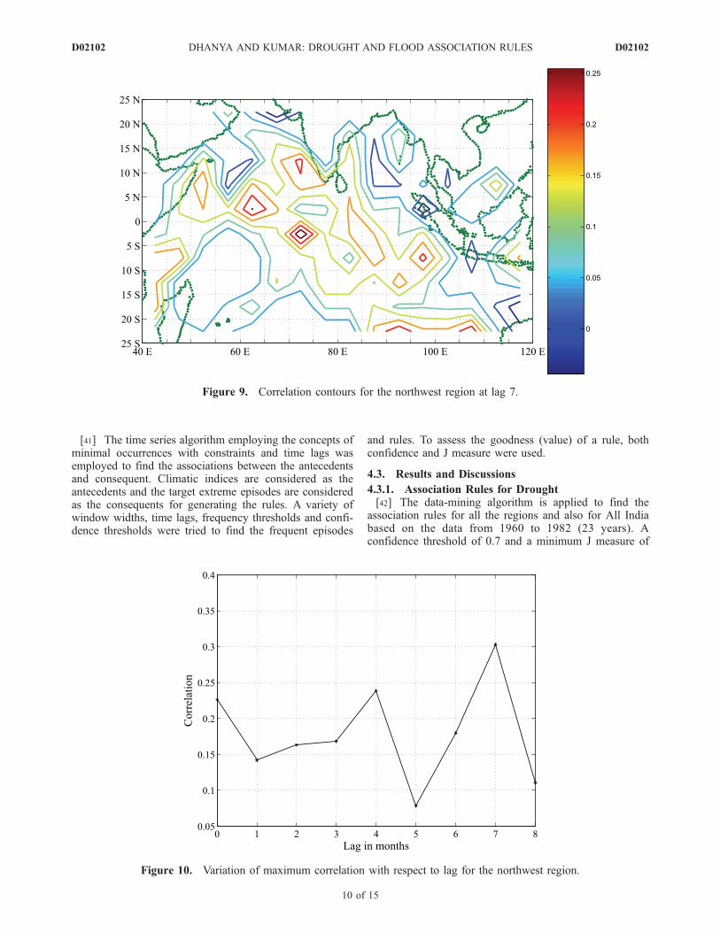
[38] 1 � 1 degree grid SST data over the region 40�E–120�E, 25�S–25�N are averaged to a 5 � 5 degree grid

data, thus reducing to 127 grids (excluding the land arearegions). Among these, the most influencing grids areselected by plotting the correlation contour plots consider-ing different lags for each region. Grids used for correlationanalysis (numbered 1 to 127) are shown in Figure 8. Themaximum correlation of SST with the summer monsoon isachieved at lag 7 for all the regions. The correlation contoursfor northwest region for lag 7 is shown in Figure 9. The

Figure 5. Summer monsoon rainfall for the northeast region for the period 1960–2005 indicating thethreshold values to classify droughts and floods.

Figure 6. Summer monsoon rainfall for the peninsular region for the period 1960–2005 indicating thethreshold values to classify droughts and floods.


8 of 15

D02102

variation of correlation versus lag for northwest region isshown in Figure 10 as an illustration.[39] The climatic indices which are used as antecedents in

rule generation are thus, DSLP, Nino 3.4, NAO and SSTvalues of those grids which are showing maximum corre-lation with the summer monsoon rainfall of each region.The most influencing grids and the corresponding maxi-mum correlation for each region are given in Table 3.

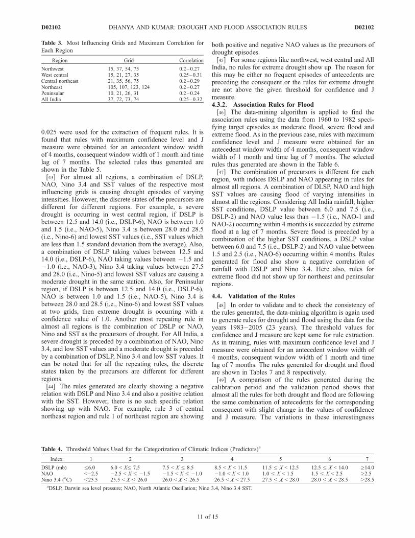
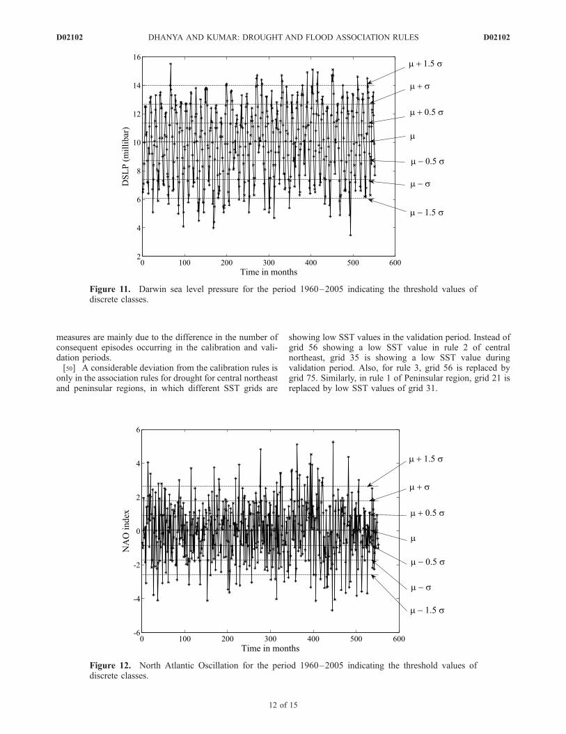
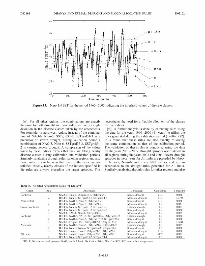
[40] The climatic indices are also categorized into sevencategories by segregating at ±1.5, ±1 and ±0.5 standarddeviations from the average. Threshold values for theseindices (except the SST grids) are given in Table 4. Thetime series of the climatic indices (DSLP, NAO and Nino3.4) for the period 1960–2005, indicating the thresholdvalues are shown in Figures 11–13.

Figure 7. Summer monsoon rainfall for All India for the period 1960–2005 indicating the thresholdvalues to classify droughts and floods.

Figure 8. SST grids of size 5� � 5� over the region 40�E–120�E, 25�S–25�N (excluding the landregions) used for correlation analysis.


9 of 15

D02102

[41] The time series algorithm employing the concepts ofminimal occurrences with constraints and time lags wasemployed to find the associations between the antecedentsand consequent. Climatic indices are considered as theantecedents and the target extreme episodes are consideredas the consequents for generating the rules. A variety ofwindow widths, time lags, frequency thresholds and confi-dence thresholds were tried to find the frequent episodes

and rules. To assess the goodness (value) of a rule, bothconfidence and J measure were used.

4.3. Results and Discussions

4.3.1. Association Rules for Drought[42] The data-mining algorithm is applied to find the

association rules for all the regions and also for All Indiabased on the data from 1960 to 1982 (23 years). Aconfidence threshold of 0.7 and a minimum J measure of

Figure 9. Correlation contours for the northwest region at lag 7.

Figure 10. Variation of maximum correlation with respect to lag for the northwest region.


10 of 15

D02102

0.025 were used for the extraction of frequent rules. It isfound that rules with maximum confidence level and Jmeasure were obtained for an antecedent window widthof 4 months, consequent window width of 1 month and timelag of 7 months. The selected rules thus generated areshown in the Table 5.[43] For almost all regions, a combination of DSLP,

NAO, Nino 3.4 and SST values of the respective mostinfluencing grids is causing drought episodes of varyingintensities. However, the discrete states of the precursors aredifferent for different regions. For example, a severedrought is occurring in west central region, if DSLP isbetween 12.5 and 14.0 (i.e., DSLP-6), NAO is between 1.0and 1.5 (i.e., NAO-5), Nino 3.4 is between 28.0 and 28.5(i.e., Nino-6) and lowest SST values (i.e., SST values whichare less than 1.5 standard deviation from the average). Also,a combination of DSLP taking values between 12.5 and14.0 (i.e., DSLP-6), NAO taking values between �1.5 and�1.0 (i.e., NAO-3), Nino 3.4 taking values between 27.5and 28.0 (i.e., Nino-5) and lowest SST values are causing amoderate drought in the same station. Also, for Peninsularregion, if DSLP is between 12.5 and 14.0 (i.e., DSLP-6),NAO is between 1.0 and 1.5 (i.e., NAO-5), Nino 3.4 isbetween 28.0 and 28.5 (i.e., Nino-6) and lowest SST valuesat two grids, then extreme drought is occurring with aconfidence value of 1.0. Another most repeating rule inalmost all regions is the combination of DSLP or NAO,Nino and SST as the precursors of drought. For All India, asevere drought is preceded by a combination of NAO, Nino3.4, and low SST values and a moderate drought is precededby a combination of DSLP, Nino 3.4 and low SST values. Itcan be noted that for all the repeating rules, the discretestates taken by the precursors are different for differentregions.[44] The rules generated are clearly showing a negative

relation with DSLP and Nino 3.4 and also a positive relationwith the SST. However, there is no such specific relationshowing up with NAO. For example, rule 3 of centralnortheast region and rule 1 of northeast region are showing

both positive and negative NAO values as the precursors ofdrought episodes.[45] For some regions like northwest, west central and All

India, no rules for extreme drought show up. The reason forthis may be either no frequent episodes of antecedents arepreceding the consequent or the rules for extreme droughtare not above the given threshold for confidence and Jmeasure.4.3.2. Association Rules for Flood[46] The data-mining algorithm is applied to find the

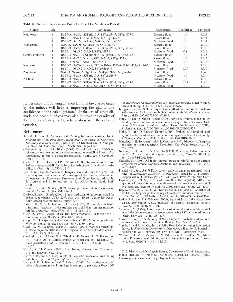
association rules using the data from 1960 to 1982 speci-fying target episodes as moderate flood, severe flood andextreme flood. As in the previous case, rules with maximumconfidence level and J measure were obtained for anantecedent window width of 4 months, consequent windowwidth of 1 month and time lag of 7 months. The selectedrules thus generated are shown in the Table 6.[47] The combination of precursors is different for each

region, with indices DSLP and NAO appearing in rules foralmost all regions. A combination of DLSP, NAO and highSST values are causing flood of varying intensities inalmost all the regions. Considering All India rainfall, higherSST conditions, DSLP value between 6.0 and 7.5 (i.e.,DSLP-2) and NAO value less than �1.5 (i.e., NAO-1 andNAO-2) occurring within 4 months is succeeded by extremeflood at a lag of 7 months. Severe flood is preceded by acombination of the higher SST conditions, a DSLP valuebetween 6.0 and 7.5 (i.e., DSLP-2) and NAO value between1.5 and 2.5 (i.e., NAO-6) occurring within 4 months. Rulesgenerated for flood also show a negative correlation ofrainfall with DSLP and Nino 3.4. Here also, rules forextreme flood did not show up for northeast and peninsularregions.

4.4. Validation of the Rules

[48] In order to validate and to check the consistency ofthe rules generated, the data-mining algorithm is again usedto generate rules for drought and flood using the data for theyears 1983–2005 (23 years). The threshold values forconfidence and J measure are kept same for rule extraction.As in training, rules with maximum confidence level and Jmeasure were obtained for an antecedent window width of4 months, consequent window width of 1 month and timelag of 7 months. The rules generated for drought and floodare shown in Tables 7 and 8 respectively.[49] A comparison of the rules generated during the

calibration period and the validation period shows thatalmost all the rules for both drought and flood are followingthe same combination of antecedents for the correspondingconsequent with slight change in the values of confidenceand J measure. The variations in these interestingness

Table 3. Most Influencing Grids and Maximum Correlation for

Each Region

Region Grid Correlation

Northwest 15, 37, 54, 75 0.2–0.27West central 15, 21, 27, 35 0.25–0.31Central northeast 21, 35, 56, 75 0.2–0.29Northeast 105, 107, 123, 124 0.2–0.27Peninsular 10, 21, 26, 31 0.2–0.24All India 37, 72, 73, 74 0.25–0.32

Table 4. Threshold Values Used for the Categorization of Climatic Indices (Predictors)a

Index 1 2 3 4 5 6 7

DSLP (mb) �6.0 6.0 < X� 7.5 7.5 < X � 8.5 8.5 < X < 11.5 11.5 � X < 12.5 12.5 � X < 14.0 14.0NAO <�2.5 �2.5 < X � �1.5 �1.5 < X � �1.0 �1.0 < X < 1.0 1.0 � X < 1.5 1.5 � X < 2.5 2.5Nino 3.4 (�C) �25.5 25.5 < X � 26.0 26.0 < X � 26.5 26.5 < X < 27.5 27.5 � X < 28.0 28.0 � X < 28.5 28.5

aDSLP, Darwin sea level pressure; NAO, North Atlantic Oscillation; Nino 3.4, Nino 3.4 SST.


11 of 15

D02102

measures are mainly due to the difference in the number ofconsequent episodes occurring in the calibration and vali-dation periods.[50] A considerable deviation from the calibration rules is

only in the association rules for drought for central northeastand peninsular regions, in which different SST grids are

showing low SST values in the validation period. Instead ofgrid 56 showing a low SST value in rule 2 of centralnortheast, grid 35 is showing a low SST value duringvalidation period. Also, for rule 3, grid 56 is replaced bygrid 75. Similarly, in rule 1 of Peninsular region, grid 21 isreplaced by low SST values of grid 31.

Figure 11. Darwin sea level pressure for the period 1960–2005 indicating the threshold values ofdiscrete classes.

Figure 12. North Atlantic Oscillation for the period 1960–2005 indicating the threshold values ofdiscrete classes.


12 of 15

D02102

[51] For all other regions, the combinations are exactlythe same for both drought and flood rules, with only a slightdeviation in the discrete classes taken by the antecedents.For example, in northwest region, instead of the combina-tion of NAO-6, Nino-5, SSTgrid37-3, SSTgrid54-3 as aprecursor of severe drought, during validation period acombination of NAO-5, Nino-6, SSTgrid37-3, SSTgrid54-2 is causing severe drought. A comparison of the valuestaken by these indices reveals that they are taking nearbydiscrete classes during calibration and validation periods.Similarly, analyzing drought rules for other regions and alsoflood rules, it can be seen that even if the rules are notsatisfied exactly, nearby classes of the indices specified inthe rules are always preceding the target episodes. This

necessitates the need for a flexible allotment of the classesfor the indices.[52] A further analysis is done by extracting rules using

the data for the years 1960–2000 (41 years) to affirm therules generated during the calibration period (1960–1982).It is found that these rules are also exactly followingthe same combination as that of the calibration period.The validation of these rules is conducted using the datafor the years 2001–2005. Drought episodes occur almost inall regions during the years 2002 and 2004. Severe droughtepisodes in these years for All India are preceded by NAO-5, Nino-5, Nino-6 and lower SST values and are inaccordance to the drought rules generated for All India.Similarly, analyzing drought rules for other regions and also

Figure 13. Nino 3.4 SST for the period 1960–2005 indicating the threshold values of discrete classes.

Table 5. Selected Association Rules for Droughta

Region Rule Antecedent Consequent Confidence J measure

Northwest 1 NAO-6, Nino-5, SSTgrid37-3, SSTgrid54-3 Severe drought 0.75 0.0382 DSLP-5, Nino-5, SSTgrid54-1, SSTgrid54-3 Moderate drought 0.75 0.0394

West central 1 DSLP-6, NAO-5, Nino-6, SSTgrid15-2 Severe drought 0.75 0.0382 DSLP-6, NAO-3, Nino-5, SSTgrid21-2 Moderate drought 1.0 0.043

Central northeast 1 DSLP-6, Nino-6, SSTgrid21-2, SSTgrid56-2 Extreme drought 1.0 0.0342 DSLP-6, Nino-5, SSTgrid21-2, SSTgrid56-3 Severe drought 1.0 0.0363 NAO-3, NAO-6, Nino-6, SSTgrid56-3 Moderate drought 1.0 0.035

Northeast 1 DSLP-5, NAO-3, NAO-5, SSTgrid105-2, SSTgrid123-2 Extreme drought 1.0 0.0362 DSLP-6, NAO-2, Nino-6, SSTgrid107-2, SSTgrid123-2 Severe drought 1.0 0.0383 NAO-7, SSTgrid105-3, SSTgrid107-3, SSTgrid123-2 Moderate drought 1.0 0.0484

Peninsular 1 DSLP-6, NAO-5, Nino-6, SSTgrid21-2, SSTgrid26-2 Extreme drought 1.0 0.0392 DSLP-6, Nino-5, Nino-6, SSTgrid26-3, SSTgrid31-2 Severe drought 1.0 0.0383 NAO-5, Nino-5, Nino-6, SSTgrid21-3, SSTgrid26-2 Moderate drought 0.75 0.038

All India 1 NAO-5, Nino-5, Nino-6, SSTgrid72-3, SSTgrid74-3 Severe drought .0.75 0.0312 DSLP-5, Nino-5, SSTgrid73-2, SSTgrid74-1 Moderate drought 1.0 0.056

aDSLP, Darwin sea level pressure; NAO, North Atlantic Oscillation; Nino, Nino 3.4 SST; SST, sea surface temperature.


13 of 15

D02102

flood rules, it can be seen that almost all the drought andflood episodes are preceded by the exact combinations ofthe climatic indices shown by the respective rules. In all thecases, either the indices are taking the exact values men-tioned in the rules or at least they are taking the nearbyclasses of the indices specified in the rules. This againdemands for a flexible allotment of the classes for theindices. Instead of defining the classes with abrupt and welldefined boundaries, a vague and ambiguous boundary bymaking use of the concept of fuzzy sets, can be used forclassifying the indices into different sets.

5. Conclusions

[53] Data mining is a powerful technology to extract thehidden predictive information from databases thus helpingin the prediction of future trends and behaviors. Data-mining tools scour databases for hidden patterns, findingpredictive information that experts may miss because it liesoutside their expectations. Implementing this technology inthe extraction of association rules for the extreme conditionsmay help decision makers to improve their fundamentalscientific understanding of drought, about its causes, pre-

dictability, impacts, mitigation actions, planning methodol-ogies, and policy alternatives.[54] Various rules generated for each region and also for

All India clearly indicate a strong relationship with climaticindices chosen, i.e., DSLP, NAO, Nino 3.4 and SST values.From the rules extracted, it can be seen that almost all theclimatic indices mentioned above are occurring as antece-dents for drought episodes, with different combinations andconfidence values. However, for rules extracted for floodepisodes, the combinations with Nino 3.4 are confrontedonly a few times.[55] The validation of the rules, using the data from 1983

to 2005, shows good consistency of the rules in thevalidation period. Almost all rules are exactly followingthe same combination as that of the calibration period rules.For some of the rules, although the combination of theindices mentioned is followed during the validation period,one or two climatic indices which are indicated as theprecursors to the extremes in the rules are not falling inthe same discrete range specified in the training period rulesor in other words they are taking the nearby discrete states.Thus a better extraction of the rules may be possible if theclassification of the indices is done in a fuzzy manner andnot in a crisp manner. This fuzzy aspect can be taken up as

Table 6. Selected Association Rules for Flood


Northwest 1 DSLP-3, NAO-5, SSTgrid15-6, SSTgrid54-5, SSTgrid75-5 Extreme flood 1.0 0.0382 DSLP-1, NAO-6, Nino-2, Nino-3, SSTgrid75-5 Severe flood 1.0 0.03763 DSLP-2, DSLP-3, NAO-3, NAO-6, SSTgrid37-5 Moderate flood 0.75 0.038

West central 1 NAO-3, NAO-6, SSTgrid21-5, SSTgrid27-6 Extreme flood 1.0 0.0362 DSLP-3, NAO-3, SSTgrid15-6, SSTgrid27-5, SSTgrid35-5 Severe flood 1.0 0.0343 DSLP-1, DSLP-2, NAO-1, SSTgrid35-5 Moderate flood 0.8 0.052

Central northeast 1 DSLP-3, NAO-3, SSTgrid21-5, SSTgrid56-5, SSTgrid75-7 Extreme flood 1.0 0.0352 DSLP-3, NAO-3, Nino-3, SSTgrid21-5, SSTgrid75-6 Severe flood 1.0 0.0423 DSLP-1, Nino-2, Nino-3, SSTgrid35-5 Moderate flood 1.0 0.060

Northeast 1 DSLP-2, NAO-6, Nino-3, SSTgrid107-5, SSTgrid123-6, SSTgrid124-5 Severe flood 1.0 0.0382 DSLP-1, DSLP-2, NAO-2, SSTgrid124-5 Moderate flood 0.75 0.036

Peninsular 1 NAO-3, Nino-3, SSTgrid10-5, SSTgrid21-5, SSTgrid26-6 Severe flood 0.75 0.0432 DSLP-1, NAO-6, SSTgrid10-5, SSTgrid26-6 Moderate flood 1.0 0.029

All India 1 DSLP-2, NAO-1, NAO-2, SSTgrid37-6 Extreme flood 1.0 0.0582 DSLP-2, NAO-6, SSTgrid37-5, SSTgrid72-5, SSTgrid73-5 Severe flood 0.83 0.0633 DSLP-2, NAO-7, Nino-3, SSTgrid37-5, SSTgrid72-5 Moderate flood 0.75 0.037

Table 7. Selected Association Rules for Drought for Validation Period


Northwest 1 NAO-5, Nino-6, SSTgrid37-3, SSTgrid54-2 Severe drought 0.75 0.0322 DSLP-6, Nino-5, SSTgrid54-1, SSTgrid54-2 Moderate drought 0.75 0.034

West central 1 DSLP-7, NAO-5, Nino-6, SSTgrid15-3 Severe drought 1.0 0.0602 DSLP-5, NAO-3, Nino-6, SSTgrid21-2 Moderate drought 0.75 0.043

Central northeast 1 DSLP-5, Nino-6, SSTgrid21-1, SSTgrid56-3 Extreme drought 1.0 0.0812 DSLP-5, Nino-5, SSTgrid21-2, SSTgrid35-3 Severe drought 0.8 0.0573 NAO-3, NAO-7, Nino-6, SSTgrid75-1 Moderate drought 1.0 0.054

Northeast 1 DSLP-5, NAO-3, NAO-5, SSTgrid105-2, SSTgrid123-2 Extreme drought 1.0 0.0522 DSLP-6, NAO-3, Nino-5, SSTgrid107-2, SSTgrid123-2 Severe drought 1.0 0.0343 NAO-6, SSTgrid105-3, SSTgrid107-1, SSTgrid123-2 Moderate drought 0.75 0.037

Peninsular 1 DSLP-6, NAO-5, Nino-6, SSTgrid26-3, SSTgrid31-2 Extreme drought 1.0 0.0392 DSLP-6, Nino-5, Nino-6, SSTgrid26-2, SSTgrid31-2 Severe drought 1.0 0.0563 NAO-5, Nino-5, Nino-6, SSTgrid21-3, SSTgrid26-3 Moderate drought 1.0 0.031

All India 1 NAO-5, Nino-5, Nino-6, SSTgrid72-2, SSTgrid74-3 Severe drought 0.75 0.0372 DSLP-5, Nino-6, SSTgrid73-1, SSTgrid74-2 Moderate drought 1.0 0.047


14 of 15

D02102

further study. Introducing an uncertainty in the classes takenby the indices will help in improving the quality andconfidence of the rules generated. Inclusion of other cli-matic and oceanic indices may also improve the quality ofthe rules in identifying the relationships with the extremeepisodes.

ReferencesBayardo, R. J., and R. Agarwal (1999), Mining the most interesting rules, inProceedings of the Fifth ACM International Conference on KnowledgeDiscovery and Data Mining, edited by S. Chaudhuri and D. Madigan,pp. 145–154, Assoc. for Comput. Mach., San Diego, Calif.

Chattopadhyay, J., and R. Bhatla (2002), Possible influence of QBO onteleconnections relating Indian summer monsoon rainfall and sea-surfacetemperature anomalies across the equatorial Pacific, Int. J. Climatol.,22(1), 121–127.

Clark, C. O., J. E. Cole, and P. J. Webster (2000), Indian ocean SST andIndian summer rainfall: Predictive relationships and their decadal varia-bility, J. Clim., 13(14), 2503–2519.

Das, G., K. I. Lin, H. Mannila, G. Ranganathan, and P. Smyth (1998), Rulediscovery from time series, in Proceedings of the Fourth InternationalConference on Knowledge Discovery and Data Mining, edited byR. Agrawal and P. Stolorz, pp. 16–22, AAAI Press, Menlo Park,Calif.

DelSole, T., and J. Shukla (2002), Linear prediction of Indian monsoonrainfall, J. Clim., 15(24), 3645–3658.

DelSole, T., and J. Shukla (2006), Linear prediction of monsoon rainfall forIndian subdivisions, COLA Tech. Rep. 208, 19 pp., Center for Ocean-Land Atmosphere Studies, Calverton, Md.

Dube, S. K., M. E. Luther, and J. O’Brien (1990), Relationships betweeninterannual variability in the Arabian Sea and Indian summer monsoonrainfall, Meteorol. Atmos. Phys., 44(1–4), 153–165.

Gadgil, S., and S. Gadgil (2006), The Indian monsoon—GDP and agricul-ture, Econ. Polit. Weekly, 41(47), 4887–4895.

Gadgil, S., M. Rajeevan, and R. Nanjunduah (2005), Monsoon prediction:Why yet another failure, Curr. Sci., 88(9), 1389–1400.

Gadgil, S., M. Rajeevan, and P. A. Francis (2007), Monsoon variability:Links to major oscillations over the equatorial Pacific and Indian oceans,Curr. Sci., 93(2), 182–194.

Goddard, L., S. J. Mason, S. E. Zebiak, C. F. Ropelewski, R. Basher, andM. A. Cane (2001), Current approaches to seasonal to inter-annual cli-mate predictions, Int. J. Climatol., 21(9), 1111–1152, doi:10.1002/joc636.

Han, J., and M. Kamber (2006), Data Mining: Concepts and Techniques,770 pp., Elsevier, New York.

Harms, S. K., and J. S. Deogun (2004), Sequential association rule miningwith time lags, J. Intelligent Inf. Syst., 22(1), 7–22.

Harms, S. K., J. Deogun, and T. Tadesse (2002), Discovering sequentialrules with constraints and time lags in multiple sequences, in Proc. 2002

Int. Symposium on Methodologies for Intelligent Systems, edited by M. S.Hacid et al., pp. 432–441, ISMIS, Lyon, France.

Iyengar, R. N., and S. T. G. Raghu Kanth (2004), Intrinsic mode functionsand a strategy for forecasting Indian monsoon rainfall, Meteorol. Atmos.Phys., doi:10.1007/s00703-004-0089-4.

Maity, R., and D. Nagesh Kumar (2006), Bayesian dynamic modeling formonthly Indian summer monsoon rainfall using El Nino-Southern Oscil-lation (ENSO) and Equatorial Indian Ocean Oscillation (EQUINOO),J. Geophys. Res., 111, D07104, doi:10.1029/2005JD006539.

Maity, R., and D. Nagesh Kumar (2008), Probabilistic prediction ofhydroclimatic variables with nonparametric quantification of uncertainty,J. Geophys. Res., 113, D14105, doi:10.1029/2008JD009856.

Mannila, H., H. Toivonen, and A. I. Verkamo (1997), Discovery of frequentepisodes in event sequences, Data Min. Knowledge Discovery, 1(3),259–289.

Navone, H. D., and H. A. Ceccatto (1994), Predicting Indian monsoonrainfall: A neural network approach, Clim. Dyn., 10(6 –7), 305–312,doi:10.1007/BF00228029.

Nicholls, N. (1995), All-India summer monsoon rainfall and sea surfacetemperatures around Northern Australia and Indonesia, J. Clim., 8(5),1463–1467.

Piatetsky-Shapiro, G. (1991), Discovery, analysis, and presentation of strongrules, in Knowledge Discovery in Databases, edited by G. Piatetsky-Shapiro and W. J. Frawley, pp. 229–248, AAAI Press, Menlo Park, Calif.

Rajeevan, M., D. S. Pai, S. K. Diskhit, and R. R. Kelkar (2004), IMD’s newoperational models for long range forecast of southwest monsoon rainfallover India and their verification for 2003, Curr. Sci., 86(3), 422–430.

Rajeevan, M., D. S. Pai, R. Anil Kumar, and B. Lal (2006), New statisticalmodels for long range forecasting of southwest monsoon rainfall overIndia, Clim. Dyn., 28(7–8), 813–828, doi:10.1007/s00382-006-0197-6.

Reddy, P. R., and P. S. Salvekar (2003), Equatorial east Indian Ocean seasurface temperature: A new predictor for seasonal and annual rainfall,Curr. Sci., 85(11), 1600–1604.

Sadhuram, Y. (2006), Long range forecast of southwest monthly rainfallover India during summer monsoon season using SST in the north IndianOcean, Curr. Sci., 91(4), 425–428.

Shukla, J., and D. A. Mooley (1987), Empirical prediction of summermonsoon rainfall over India, Mon. Weather Rev., 115, 695–703.

Smyth, P., and R. M. Goodman (1991), Rule induction using informationtheory, in Knowledge Discovery in Databases, edited by G. Piatetsky-Shapiro and W. J. Frawley, pp. 159–176, MIT, Cambridge, Mass.

Webster, P. J., V. O. Magana, T. N. Palmer, and J. Shukla (1998), Mon-soons: Processes, predictability, and the prospects for prediction, J. Geo-phys. Res., 103(C7), 14,451–14,510.

��C. T. Dhanya and D. Nagesh Kumar, Department of Civil Engineering,

Indian Institute of Science, Bangalore, Karnataka 560012, India.([email protected]; [email protected])

Table 8. Selected Association Rules for Flood for Validation Period


Northwest 1 DSLP-3, NAO-5, SSTgrid15-5, SSTgrid54-5, SSTgrid75-7 Extreme flood 1.0 0.0382 DSLP-1, NAO-6, Nino-2, Nino-3, SSTgrid75-6 Severe flood 1.0 0.0413 DSLP-2, DSLP-3, NAO-3, NAO-6, SSTgrid37-5 Moderate flood 0.71 0.031

West central 1 NAO-3, NAO-6, SSTgrid21-7, SSTgrid27-7 Extreme flood 1.0 0.0422 DSLP-3, NAO-2, SSTgrid15-5, SSTgrid27-5, SSTgrid35-7 Severe flood 1.0 0.0393 DSLP-1, DSLP-2, NAO-1, SSTgrid35-6 Moderate flood 0.8 0.046

Central northeast 1 DSLP-3, NAO-3, SSTgrid21-7, SSTgrid56-6, SSTgrid75-5 Extreme flood 1.0 0.0452 DSLP-3, NAO-3, Nino-3, SSTgrid21-5, SSTgrid75-6 Severe flood 1.0 0.0353 DSLP-2, Nino-2, Nino-3, SSTgrid35-7 Moderate flood 1.0 0.044

Northeast 1 DSLP-2, NAO-6, Nino-3, SSTgrid107-6, SSTgrid123-6, SSTgrid124-5 Severe flood 1.0 0.0382 DSLP-1, DSLP-2, NAO-2, SSTgrid124-6 Moderate flood 0.75 0.039

Peninsular 1 NAO-3, Nino-2, SSTgrid10-7, SSTgrid21-5, SSTgrid26-5 Severe flood 1.0 0.0432 DSLP-2, NAO-6, SSTgrid10-5, SSTgrid26-5 Moderate flood 1.0 0.034

All India 1 DSLP-2, NAO-2, NAO-3, SSTgrid37-7 Extreme flood 1.0 0.0482 DSLP-2, NAO-7, SSTgrid37-6, SSTgrid72-5, SSTgrid73-6 Severe flood 0.75 0.0403 DSLP-2, NAO-7, Nino-3, SSTgrid37-5, SSTgrid72-5 Moderate flood 1.0 0.030


15 of 15

D02102

Data mining for evolution of association rules for...

Documents

Transcript of Data mining for evolution of association rules for...