“Data Mining”

COPPE/UFRJ/nttwww.ntt.ufrj.br

Nelson F. F. Ebeckennelson@ntt.ufrj.br

The Evolution of Science

Data Exploration Science- Data captured by instrumentsOr data generated by simulator

- Processed by software- Placed in a database / files- Scientist analyzes database/files

• Observational Science – Scientist gathers data by

direct observation– Scientist analyzes data

• Analytical Science – Scientist builds analytical

model– Makes predictions.

• Computational Science – Simulate analytical model– Validate model and makes

predictions

Information Avalanche• Both

– better observational instruments and – Better simulations are producing a data avalanche

• Examples– Turbulence: 100 TB simulation

then mine the Information – BaBar: Grows 1TB/day

2/3 simulation Information 1/3 observational Information

– CERN: LHC will generate 1GB/s10 PB/y

– VLBA (NRAO) generates 1GB/s today– NCBI: “only ½ TB” but doubling each year, very rich dataset.– Pixar: 100 TB/Movie

Image courtesy of C. Meneveau & A. Szalay @ JHU

Computational Science Evolves • Historically, Computational Science = simulation.• New emphasis on informatics:

– Capturing, – Organizing, – Summarizing, – Analyzing, – Visualizing

• Largely driven by observational science, but also needed by simulations.

• Too soon to say if comp-X and X-info will unify or compete.

BaBar, Stanford

P&E Gene SequencerFromhttp://www.genome.uci.edu/

Space Telescope

Next-Generation Data Analysis• As data and computers grow at same rate…

• A way out? – Discard notion of optimal (data is fuzzy, answers

are approximate)– Don’t assume infinite computational resources or

memory• Requires combination of statistics & computer

science

Organization & Algorithms• Use of clever data structures (trees, cubes):

– Large speedup during the analysis– Tree-codes for correlations – Data Cubes for OLAP (all vendors)

• Fast, approximate heuristic algorithms– No need to be more accurate than data variance

• Take cost of computation into account– Controlled level of accuracy– Best result in a given time, given our computing resources

• Use parallelism– Many disks– Many cpus

Analysis and Databases• Much statistical analysis deals with

– Creating uniform samples –– data filtering– Assembling relevant subsets– Estimating completeness – censoring bad data– Counting and building histograms– Generating Monte-Carlo subsets– Likelihood calculations– Hypothesis testing

• Traditionally these are performed on files• Most of these tasks are much better done inside DB

Information => Data => Knowledge

● KDD (Knowledge Discovery on Databases) does not exist in a vacuum– External forces can have more impact on the field

than internal forces● KDD is a young field with little history to guide it

- in contrast the American Statistical Association is meeting for their 166nd annual meeting this year

● Predicting the future is hard even with historical data

Reason for Data Model

Data = $$

Within the scientific community:- the data is much more dispersed- the goal in modeling scientific problems was to find and to formulate governing laws in the form of precise mathematical terms.

• It has long been recognized that such perfect descriptions are not always possible. Incomplete and imprecise knowledge, observations that are often of a qualitative nature, the great heterogeneity of the surrounding world, boundaries and initial conditions being not completely know, all this generate the search for data models.

• To build a model that does not need complex mathematical equations, one needs sufficient and good data.

Motivation

• Data explosion problem

– Automated data collection tools and mature database technology

lead to tremendous amounts of data stored in databases, data

warehouses and other information repositories

• We are drowning in data, but starving for knowledge!

• Solution: Data warehousing and data mining

– Data warehousing and on-line analytical processing

– Extraction of interesting knowledge (rules, regularities, patterns,

constraints) from data in large databases

Evolution of Database Technology• 1960s:

– Data collection, database creation, IMS and network DBMS• 1970s:

– Relational data model, relational DBMS implementation• 1980s:

– RDBMS, advanced data models (extended-relational, OO, deductive, etc.) and application-oriented DBMS (spatial, scientific, engineering, etc.)

• 1990s—2000s: – Data mining and data warehousing, multimedia databases, and

Web databases– Oracle Data Mining, MS SQL Server, IBM DB2,…– Free and opened databases

What Is Data Mining?• Data mining (knowledge discovery in databases):

– Extraction of interesting (non-trivial, implicit, previously unknownand potentially useful) information or patterns from data in large databases

• What is not data mining?– (Deductive) query processing. – Expert systems or small ML/statistical programs– …..– …..– Unstructured queries, OLAP(on line analytical processing)

differs from SQL queries in the level of abstraction, or “open ended-ness” that can be included in the query

– …..

Potential Applications

• Database analysis and decision support– Market analysis and management

– Risk analysis and management

– …..

• New Applications– Text mining (documents…)

– Web mining

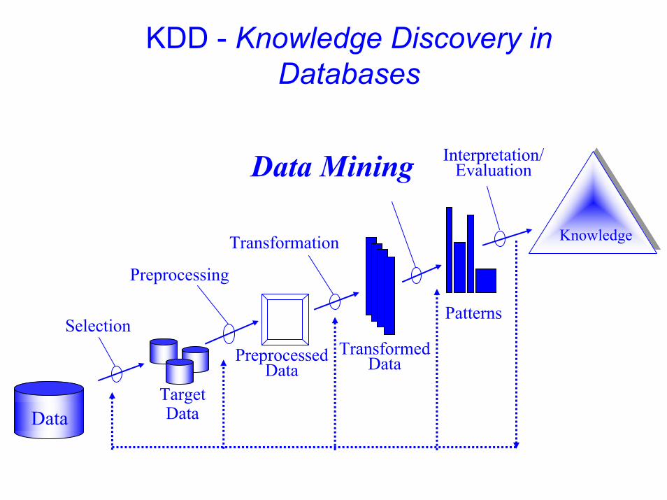
KDD - Knowledge Discovery in Databases

Data

Knowledge

Transformed Data

Patterns

Target Data

Preprocessed Data

Selection

Preprocessing

Transformation

Data Mining Interpretation/Evaluation

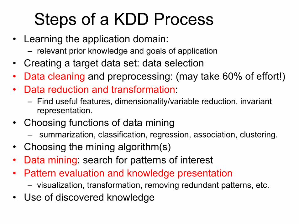
Steps of a KDD Process• Learning the application domain:

– relevant prior knowledge and goals of application• Creating a target data set: data selection• Data cleaning and preprocessing: (may take 60% of effort!)• Data reduction and transformation:

– Find useful features, dimensionality/variable reduction, invariant representation.

• Choosing functions of data mining – summarization, classification, regression, association, clustering.

• Choosing the mining algorithm(s)• Data mining: search for patterns of interest• Pattern evaluation and knowledge presentation

– visualization, transformation, removing redundant patterns, etc.• Use of discovered knowledge

Multiple Disciplines

Data Mining

Database Technology Statistics

MachineLearning Visualization

InformationScience

OtherDisciplines

Major Tasks in Data Preprocessing

• Data cleaning– Fill in missing values, smooth noisy data, identify or remove

outliers, and resolve inconsistencies

• Data integration– Integration of multiple databases, data cubes, or files

• Data transformation– Normalization and aggregation

• Data reduction– Obtains reduced representation in volume but produces the

same or similar analytical results

• Data discretization– Part of data reduction but with particular importance, especially

for numerical data

Data Mining Functionalities • Concept description: Characterization and discrimination

– Generalize, summarize, and contrast data characteristics.

• Association (correlation and causality)– Multi-dimensional vs. single-dimensional association

• Antecedent (X)=> Consequent (Y)• Rule 13 (1266 registers):• Cumulative Rain 6 days [> 92.6 mm] => ACCIDENT• (25,5% 91.9% 323 297 23.5%)

• 25.5% - rule support [P (X U Y)]• 91.9% - confidence [P (Y|X)] • 323 - number of occurrences on the union • 297 - number of occurrences on the intersection • 23.5% - percentage of the intersection

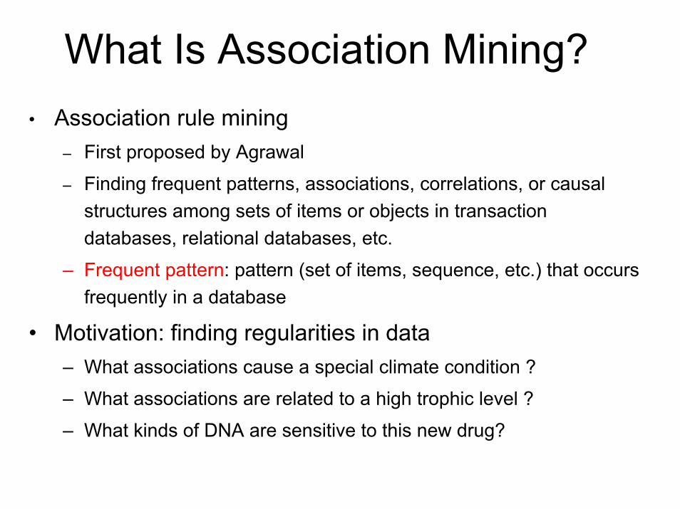
What Is Association Mining?• Association rule mining

– First proposed by Agrawal

– Finding frequent patterns, associations, correlations, or causalstructures among sets of items or objects in transaction databases, relational databases, etc.

– Frequent pattern: pattern (set of items, sequence, etc.) that occurs frequently in a database

• Motivation: finding regularities in data– What associations cause a special climate condition ?

– What associations are related to a high trophic level ?

– What kinds of DNA are sensitive to this new drug?

Visualization of Association Rules

Classification and Prediction

• Classification:– predicts categorical class labels (discrete or

nominal)– classifies data (constructs a model) based on the

training set and the values (class labels) in a classifying attribute and uses it in classifying new data

• Prediction:– models continuous-valued functions, i.e., predicts

unknown or missing values

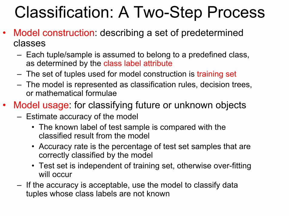
Classification: A Two-Step Process• Model construction: describing a set of predetermined

classes– Each tuple/sample is assumed to belong to a predefined class,

as determined by the class label attribute– The set of tuples used for model construction is training set– The model is represented as classification rules, decision trees,

or mathematical formulae• Model usage: for classifying future or unknown objects

– Estimate accuracy of the model• The known label of test sample is compared with the

classified result from the model• Accuracy rate is the percentage of test set samples that are

correctly classified by the model• Test set is independent of training set, otherwise over-fitting

will occur– If the accuracy is acceptable, use the model to classify data

tuples whose class labels are not known

Supervised and Unsupervised Learning

• Supervised learning (classification)– Supervision: The training data (observations,

measurements, etc.) are accompanied by labels indicating the class of the observations

– New data is classified based on the training set

• Unsupervised learning (clustering)– The class labels of training data is unknown

– Given a set of measurements, observations, etc. with the aim of establishing the existence of classes or clusters in the data

A Decision Tree

INDEX ?

overcast

AX?

CY?

no yes fairexcellent

<=10 >30

no noyes yes

B

10..30

Algorithm for Decision Tree Induction

• Basic algorithm (a greedy algorithm)– Tree is constructed in a top-down recursive divide-and-conquer

manner– At start, all the training examples are at the root– Attributes are categorical (if continuous-valued, they are

discretized in advance)– Examples are partitioned recursively based on selected

attributes– Test attributes are selected on the basis of a heuristic or

statistical measure (ex., information gain)• Conditions for stopping partitioning

– All samples for a given node belong to the same class– There are no remaining attributes for further partitioning –

majority voting is employed for classifying the leaf– There are no samples left

Other Attribute Selection Measures

• Gini index (CART, IBM IntelligentMiner)– All attributes are assumed continuous-valued– Assume there exist several possible split values for

each attribute– May need other tools, such as clustering, to get the

possible split values– Can be modified for categorical attributes

Extracting Classification Rules from Trees

• Represent the knowledge in the form of IF-THEN rules• One rule is created for each path from the root to a leaf• Each attribute-value pair along a path forms a

conjunction• The leaf node holds the class prediction• Rules are easier for humans to understand• Example

IF X = “<= C” AND Y = “no” THEN Y = “no”

Presentation of Classification Results

Decision Tree in SGI/MineSet

Bayesian Classification• Probabilistic learning: Calculate explicit probabilities for

hypothesis, among the most practical approaches to certain types of learning problems

• Incremental: Each training example can incrementally increase/decrease the probability that a hypothesis is correct. Prior knowledge can be combined with observed data.

• Probabilistic prediction: Predict multiple hypotheses, weighted by their probabilities

• Standard: Even when Bayesian methods are computationally intractable, they can provide a standard of optimal decision making against which other methods can be measured

Naïve Bayes Classifier • A simplified assumption: attributes are

conditionally independent:

• The product of occurrence of say 2 elements x1 and x2, given the current class is C, is the product of the probabilities of each element taken separately, given the same class P([y1,y2],C) = P(y1,C) * P(y2,C)

• No dependence relation between attributes • Greatly reduces the computation cost, only count the

class distribution.• Once the probability P(X|Ci) is known, assign X to the

class with maximum P(X|Ci)*P(Ci)

∏=

=n

kCixkPCiXP

1)|()|(

Naïve Bayesian Classifier: Comments

• Advantages : – Easy to implement – Good results obtained in most of the cases

• Disadvantages– Assumption: class conditional independence , therefore loss of

accuracy– Practically, dependencies exist among variables – E.g., hospitals: patients: Profile: age, family history etc

Symptoms: fever, cough etc., Disease: lung cancer, diabetes etc – Dependencies among these cannot be modeled by Naïve

Bayesian Classifier

• How to deal with these dependencies?– Bayesian Belief Networks

Bayesian Networks• Bayesian belief network allows a subset of the

variables conditionally independent

• A graphical model of causal relationships– Represents dependency among the variables – Gives a specification of joint probability distribution

X Y

ZP

Nodes: random variablesLinks: dependencyX,Y are the parents of Z, and Y is the

parent of PNo dependency between Z and PHas no loops or cycles

Neural Networks

• Analogy to Biological Systems (Indeed a great example of a good learning system)

• Massive Parallelism allowing for computational efficiency

• The first learning algorithm came in 1959 (Rosenblatt) who suggested that if a target output value is provided for a single neuron with fixed inputs, one can incrementally change weights to learn to produce these outputs using the perceptron learning rule

Network Training• The ultimate objective of training

– obtain a set of weights that makes almost all the tuples in the training data classified correctly

• Steps– Initialize weights with random values – Feed the input tuples into the network one by one– For each unit

• Compute the net input to the unit as a linear combination of all the inputs to the unit

• Compute the output value using the activation function• Compute the error• Update the weights and the bias

SVM – Support Vector MachinesIn very simple terms an SVM corresponds to a linear method in a very high dimensional feature space

that is nonlinearly related to the input space. Even though we think of it as a linear algorithm in a high dimensional feature space, in practice, it does not involve any computations in that high dimensional space. By the use of kernels, all necessary computations are performed directly in input space!

Support Vectors

Small Margin Large Margin

SVM vs. Neural Network

• Neural Network– Quiet Old– Generalizes well but

doesn’t have strong mathematical foundation

– Can easily be learned in incremental fashion

– To learn complex functions – use multilayer perceptron(not that trivial)

• SVM– Relatively new concept– Nice Generalization

properties– Hard to learn – learned in

batch mode using quadratic programming techniques

– Using kernels can learn very complex functions

The k-Nearest Neighbor Algorithm• All instances correspond to points in the n-D space.• The nearest neighbor are defined in terms of Euclidean distance.• The target function could be discrete - or real- valued.

• The k-NN algorithm for continuous-valued target functions– Calculate the mean values of the k nearest neighbors

• Distance-weighted nearest neighbor algorithm– Weight the contribution of each of the k neighbors according to their

distance to the query point– giving greater weight to closer neighbors– Similarly, for real-valued target functions

• Robust to noisy data by averaging k-nearest neighbors• Curse of dimensionality: distance between neighbors could be

dominated by irrelevant attributes. To overcome it, axes stretch or elimination of the least relevant attributes.

• Genetic Algorithms: were used in optimization and search problems arrive at a near optimal solution in a relatively short time. More recently GAs have been considered for use in data mining using different approaches.– In conjunction with existing classification algorithms-by finding near optimal

solution the GA can narrow the search space of possible solutions to which the traditional system is then applied, the resultant hybrid approach presenting a more efficient solution to problems in large domains.

– GAs have been used as post-processors of classification models - neural networks, decision-trees and decision-rules are structures that can be adapted; by coding these structures it is possible to optimize their performance, e.g. in a neural network the number and organization of neural may be adapted.

• GAs may be used in the building of classifier systems - genetic-based decision rules that classify in their own right (clustering and prediction).

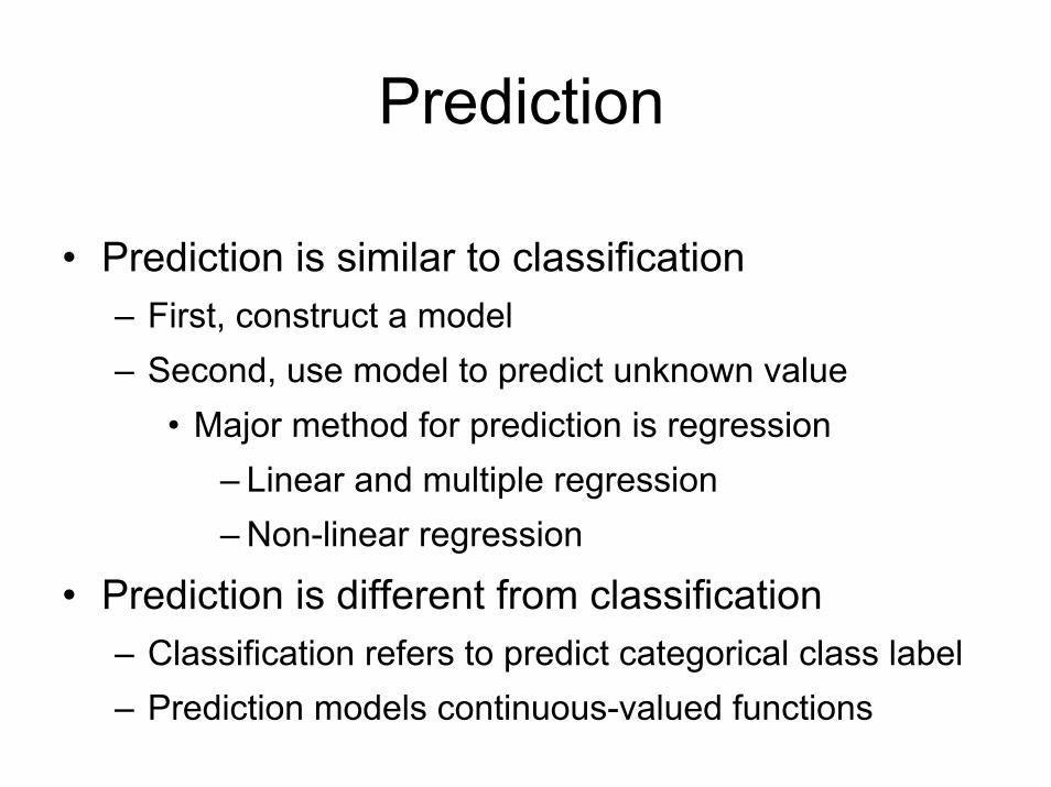
Prediction

• Prediction is similar to classification– First, construct a model– Second, use model to predict unknown value

• Major method for prediction is regression– Linear and multiple regression– Non-linear regression

• Prediction is different from classification– Classification refers to predict categorical class label– Prediction models continuous-valued functions

Prediction: Numerical Data

Classification Accuracy: Estimating Error Rates

• Partition: Training-and-testing– use two independent data sets, e.g., training set (2/3),

test set(1/3)– used for data set with large number of samples

• Cross-validation– divide the data set into k subsamples– use k-1 subsamples as training data and one sub-

sample as test data—k-fold cross-validation– for data set with moderate size

• Bootstrapping (leave-one-out)– for small size data

Bagging and Boosting

• General idea Training data

Altered Training data

Altered Training data……..Aggregation ….

Classification method (CM)

Classifier C

CM

Classifier C1

CM

Classifier C2

Classifier C*

Bagging • Given a set S of s samples • Generate a bootstrap sample T from S. Cases in S may

not appear in T or may appear more than once. • Repeat this sampling procedure, getting a sequence of k

independent training sets• A corresponding sequence of classifiers C1,C2,…,Ck is

constructed for each of these training sets, by using the same classification algorithm

• To classify an unknown sample X,let each classifier predict or vote

• The Bagged Classifier C* counts the votes and assigns X to the class with the “most” votes

Boosting Technique — Algorithm

• Assign every example an equal weight 1/N• For t = 1, 2, …, T Do

– Obtain a hypothesis (classifier) h(t) under w(t)

– Calculate the error of h(t) and re-weight the examples based on the error . Each classifier is dependent on the previous ones. Samples that are incorrectly predicted are weighted more heavily

– Normalize w(t+1) to sum to 1 (weights assigned to different classifiers sum to 1)

• Output a weighted sum of all the hypothesis, with each hypothesis weighted according to its accuracy on the training set

What is Cluster Analysis?

• Cluster: a collection of data objects– Similar to one another within the same cluster– Dissimilar to the objects in other clusters

• Cluster analysis– Grouping a set of data objects into clusters

• Clustering is unsupervised classification: no predefined classes

• Typical applications– As a stand-alone tool to get insight into data distribution – As a preprocessing step for other algorithms

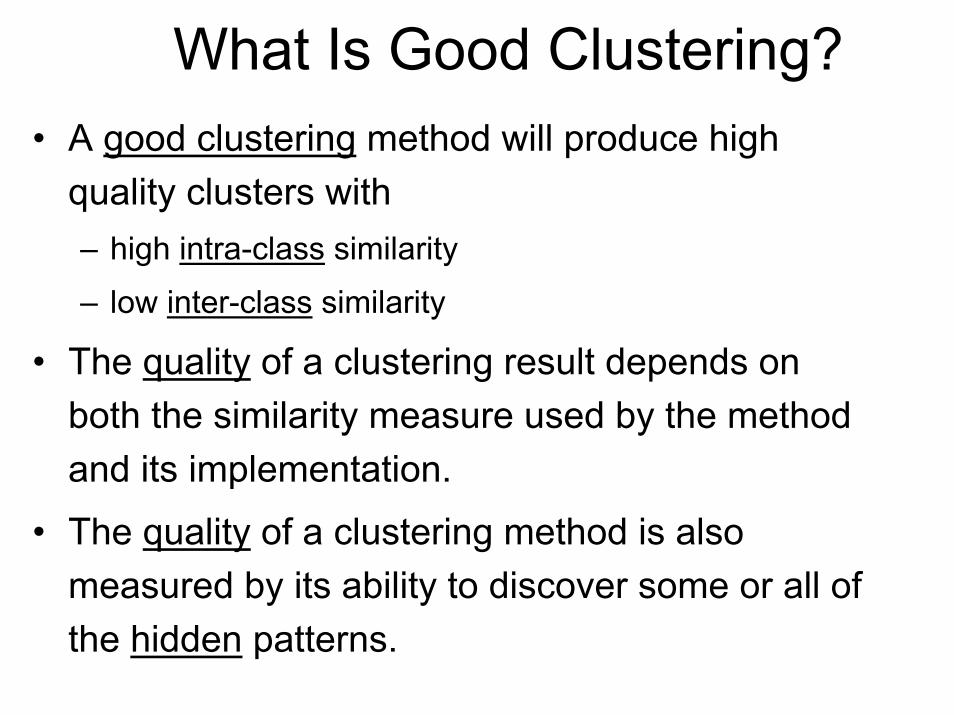
What Is Good Clustering?• A good clustering method will produce high

quality clusters with– high intra-class similarity

– low inter-class similarity

• The quality of a clustering result depends on both the similarity measure used by the method and its implementation.

• The quality of a clustering method is also measured by its ability to discover some or all of the hidden patterns.

Major Clustering Approaches• Partitioning algorithms: Construct various partitions and

then evaluate them by some criterion

• Hierarchy algorithms: Create a hierarchical decomposition of the set of data (or objects) using some criterion

• Density-based: based on connectivity and density functions

• Grid-based: based on a multiple-level granularity structure

• Model-based: A model is hypothesized for each of the clusters and the idea is to find the best fit of that model to each other

The K-Means Clustering Method

• Given k, the k-means algorithm is implemented in four steps:– Partition objects into k nonempty subsets

– Compute seed points as the centroids of the clusters of the current partition (the centroid is the center, i.e., mean point, of the cluster)

– Assign each object to the cluster with the nearest seed point

– Go back to Step 2, stop when no more new assignment

The K-Means Clustering Method• Example

0

1

2

3

4

5

6

7

8

9

10

0 1 2 3 4 5 6 7 8 9 100

1

2

3

4

5

6

7

8

9

10

0 1 2 3 4 5 6 7 8 9 100

1

2

3

4

5

6

7

8

9

10

0 1 2 3 4 5 6 7 8 9 10

Update the cluster means

Assign each objects to most similar center

0

1

2

3

4

5

6

7

8

9

10

0 1 2 3 4 5 6 7 8 9 10

reassign reassign

0

1

2

3

4

5

6

7

8

9

10

0 1 2 3 4 5 6 7 8 9 10

K=2

Arbitrarily choose K object as initial cluster center Update

the cluster means

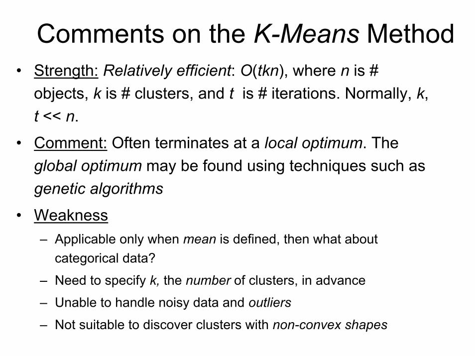
Comments on the K-Means Method• Strength: Relatively efficient: O(tkn), where n is #

objects, k is # clusters, and t is # iterations. Normally, k, t << n.

• Comment: Often terminates at a local optimum. The global optimum may be found using techniques such as genetic algorithms

• Weakness– Applicable only when mean is defined, then what about

categorical data?

– Need to specify k, the number of clusters, in advance

– Unable to handle noisy data and outliers

– Not suitable to discover clusters with non-convex shapes

Hierarchical Clustering• Use distance matrix as clustering criteria. This method

does not require the number of clusters k as an input, but needs a termination condition

Step 0 Step 1 Step 2 Step 3 Step 4

b

dc

e

a a b

d ec d e

a b c d e

Step 4 Step 3 Step 2 Step 1 Step 0

agglomerative(AGNES)

divisive(DIANA)

A Dendrogram Shows How the Clusters are Merged Hierarchically

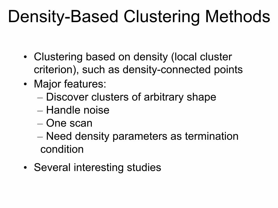
Density-Based Clustering Methods

• Clustering based on density (local cluster criterion), such as density-connected points

• Major features:– Discover clusters of arbitrary shape– Handle noise– One scan– Need density parameters as terminationcondition

• Several interesting studies

Grid-Based Clustering Method

• Using multi-resolution grid data structure

• Several interesting methods

– Statistical Information Grid approach,

– Multi-resolution clustering approach using wavelet method

– ……

Other Model-Based Clustering Methods

• Neural network approaches– Represent each cluster as an exemplar, acting as a

“prototype” of the cluster– New objects are distributed to the cluster whose

exemplar is the most similar according to some distance measure

• Competitive learning– Involves a hierarchical architecture of several units

(neurons)– Neurons compete in a “winner-takes-all” fashion for

the object currently being presented

Self-organizing feature maps (SOMs)

• Clustering is also performed by having several units competing for the current object

• The unit whose weight vector is closest to the current object wins

• The winner and its neighbors learn by having their weights adjusted

• SOMs are believed to resemble processing that can occur in the brain

• Useful for visualizing high-dimensional data in 2-or 3-D space

CLUTO VIZUALIZATIONwww-users.cs.umn.edu/~karypis/cluto/

Matrix

Mountain

What Is Outlier Discovery?

• What are outliers?– The set of objects are considerably dissimilar from the

remainder of the data– Outlier: a data object that does not comply with the general

behavior of the data

– It can be considered as noise or exception but is quite useful rare events analysis

• Problem– Find top n outlier points

Outlier Discovery: Statistical

Approaches

Assume a model underlying distribution that generates data set (e.g. normal distribution)

• Use discordancy tests depending on – data distribution– distribution parameter (e.g., mean, variance)– number of expected outliers

• Drawbacks– most tests are for single attribute– In many cases, data distribution may not be known

Outlier Discovery:Distance-Based Approach• Introduced to counter the main limitations imposed by

statistical methods- multi-dimensional analysis without knowing data

distribution.• Distance-based outlier: at least a fraction of the objects lies

at a distance greater than D from the object

Outlier Discovery:Deviation-Based Approach• Identifies outliers by examining the main characteristics of objects in a group

• Objects that “deviate” from this description are considered outliers

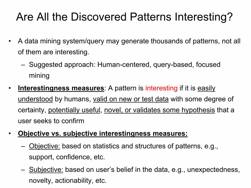
Are All the Discovered Patterns Interesting?

• A data mining system/query may generate thousands of patterns, not all of them are interesting.

– Suggested approach: Human-centered, query-based, focused mining

• Interestingness measures: A pattern is interesting if it is easily understood by humans, valid on new or test data with some degree of certainty, potentially useful, novel, or validates some hypothesis that a user seeks to confirm

• Objective vs. subjective interestingness measures:

– Objective: based on statistics and structures of patterns, e.g., support, confidence, etc.

– Subjective: based on user’s belief in the data, e.g., unexpectedness, novelty, actionability, etc.

Applications• Nowadays Data Mining is fully developed, very powerful and ready to be

used. Data Mining finds applications in many areas. The more popular are:• Data Mining on Government: Detection and Prevention of Fraud and Money

Laundering, Criminal Patterns, Health Care Transactions, etc..• Data Mining for Competitive Intelligence: CRM, New Product Ideas, Retail

Marketing and Sales Pattern, Competitive Decisions, Future Trends and Competitive Opportunities, etc..

• Data Mining on Finance: Consumer Credit Policy, Portfolio Management, Bankruptcy Prediction, Foreign Exchange Forecasting, Derivatives Pricing, Risk Management, Price Prediction, Forecasting Macroeconomic Data, Time Series Modeling, etc..

• Building Models from Data: Applications of Data Mining in Science, Engineering, Medicine, Global Climate Change Modeling, Ecological Modeling, etc..

Data Mining SystemArchitectures

• Coupling data mining system with DB/DW system– No coupling—flat file processing, not recommended– Loose coupling

• Fetching data from DB/DW

– Semi-tight coupling—enhanced DM performance• Provide efficient implement a few data mining primitives in a

DB/DW system, e.g., sorting, indexing, aggregation, histogram analysis, multiway join, precomputation of some stat functions

– Tight coupling—A uniform information processing environment

• DM is smoothly integrated into a DB/DW system, mining query is optimized based on mining query, indexing, query processing methods, etc.

MS SQL SERVER• Microsoft® (MS) Object Linking and Embedding

Database for DM (OLE DB DM) technology provides an industry standard for developing DM algorithms. This technology was included in the 2000 release of the MS SQL Server™ (MSSQL). The Analysis Services (AS) component of this software includes a DM provider supporting two algorithms: one for classification by decision trees and another for clustering. The DM Aggregator feature of this component and the OLE DB DM Sample Provider made possible for developers and researchers to implement new DM algorithms.

• The MSSQL 2005 version has included more five algorithms: Naïve Bayes, Association, Sequence Clustering, Time Series and Neural Net as well as a new way to aggregate new algorithms, using a plug-in approach instead of DM providers.

Incremental and Parallel Mining of Concept Description

• Incremental mining: revision based on newly added data ∆DB– Generalize ∆DB to the same level of abstraction in

the generalized relation R to derive ∆R– Union R U ∆R, i.e., merge counts and other statistical

information to produce a new relation R’

• Similar philosophy can be applied to data sampling, parallel and/or distributed mining, etc.

Multi-relational DM • The common approach to solve this problem is to use a

single flat table assembled by performing a relational join operation on the tables. But this approach may produce an extremely large and impractical to handle table, with lots of repeated and null data.

• In consequence, multi-relational DM (MRDM) approaches have been receiving considerable attention in the literature. These approaches rely on developing specific algorithms to deal with the relational feature of the data.

• By another way, OLE DB DM technology supports nested tables (also know as table columns). The row sets represent uniquely the tables in a nested way. There are no redundant or null data in each row set. Ex. one row per customer is all that is needed, and the nested columns of the row set contain the data pertinent to that customer.

Data Mining: Concepts and Techniques

Jiawei Han and Micheline Kamber

Data Mining: Concepts and Techniques,

The Morgan Kaufmann Series in Data Management Systems, Jim Gray, Series Editor Morgan Kaufmann Publishers, August 2000. 550 pages. ISBN 1-55860-489-8

http://www.cs.sfu.ca/~han/dmbook

Sistemas Inteligentes: Fundamentos e Aplicações

Organizadora: Solange Oliveira RezendeISBN 1683-7, ano 2002.Editora Manole

Sistemas Baseados em Conhecimento Aquisição de Conhecimento Conceitos sobre Aprendizado de Máquina Indução de Regras e Árvores de Decisão Redes Neurais Artificiais Sistemas FuzzySistemas Neuro FuzzyComputação Evolutiva Sistemas Inteligentes Híbridos Agentes e Multiagentes Mineração de DadosMineração de Texto