Data Mining - 2011 - Volinsky - Columbia University 1 Chapter 4.2 Regression Topics Credits Hastie,...
51
Data Mining - 2011 - Volinsky - Columbia University 1 Chapter 4.2 Regression Topics Credits Hastie, Tibshirani, Friedman Chapter 3 Padhraic Smyth Lecture Notes Wolfgang Jank Lecture Notes
-
Upload
rudolph-stafford -
Category
Documents
-
view
219 -
download
2
Transcript of Data Mining - 2011 - Volinsky - Columbia University 1 Chapter 4.2 Regression Topics Credits Hastie,...

Data Mining - 2011 - Volinsky - Columbia University 1
Chapter 4.2 Regression Topics
CreditsHastie, Tibshirani, Friedman Chapter 3
Padhraic Smyth Lecture NotesWolfgang Jank Lecture Notes

Data Mining - 2011 - Volinsky - Columbia University 2
Regression Review• Linear Regression models a numeric outcome as a
linear function of several predictors.• It is the king of all statistical and data mining models
– ease of interpretation– mathematically concise– tends to perform well for prediction, even under violations
of assumptions
• Characteristics– numeric response - ideally real valued– numeric predictors- but not necessarily
Data Mining - 2011 - Volinsky - Columbia University 3
Linar Regression Model
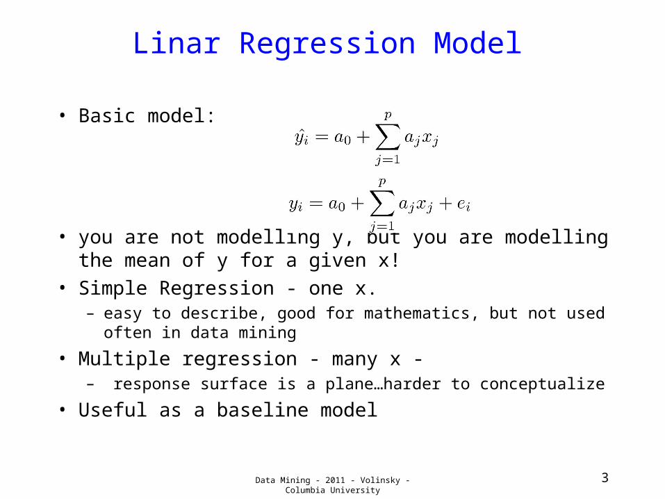
• Basic model:
• you are not modelling y, but you are modelling the mean of y for a given x!
• Simple Regression - one x. – easy to describe, good for mathematics, but not used
often in data mining
• Multiple regression - many x -– response surface is a plane…harder to conceptualize
• Useful as a baseline model

Data Mining - 2011 - Volinsky - Columbia University 4
Linear Regression Model
• Assumptions:– linearity– constant variance– normality of errors
• residuals ~ Normal(mu,sigma^2)
• Assumptions must be checked,– but if inference is not the goal, you can
accept some deviation from assumptions (don’t’ tell the statisticians I said that!)
• Multicollinearity also an issue– creates unstable estimates

Data Mining - 2011 - Volinsky - Columbia University 5
Fitting the Model
• We can look at regression as a matrix problem
• We want a score function which minimizes “a”:
=
which is minimized by

Fitting models: in-sample
Minimize the sum of the squared errors:
• S = e2 = e’ e = (y – X a)’ (y – X a)
• = y’ y – a’ X’ y – y’ X a + a’ X’ X a
• = y’ y – 2 a’ X’ y + a’ X’ X a
Take derivative of S with respect to a:• dS/da = -2X’y + 2 X’ X a
Set this to 0 to find the (minimum) of S as a function of a…
- 2X’y + 2 X’ X a = 0 X’Xa = X’ y
a = ( X’ X )-1 X’ y
Prediction follows easily:
Data Mining - 2011 - Volinsky - Columbia University
€
ˆ y k =Xka
6
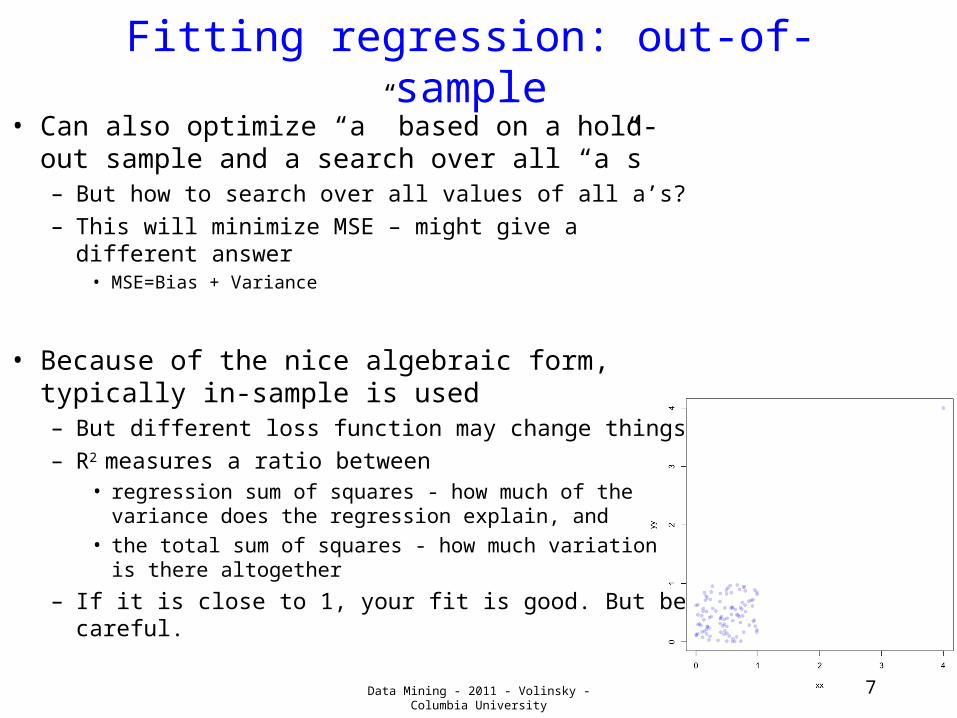
Fitting regression: out-of-sample• Can also optimize “a” based on a hold-out
sample and a search over all “a”s– But how to search over all values of all a’s?– This will minimize MSE – might give a different
answer• MSE=Bias + Variance
• Because of the nice algebraic form, typically in-sample is used– But different loss function may change things– R2 measures a ratio between
• regression sum of squares - how much of the variance does the regression explain, and
• the total sum of squares - how much variation is there altogether
– If it is close to 1, your fit is good. But be careful.
Data Mining - 2011 - Volinsky - Columbia University 7
Data Mining - 2011 - Volinsky - Columbia University 8
Limitations of Linear Regression
• True relationship of X and Y might be non-linear– Suggests generalizations to non-linear models
• Correlation/Collinearity among the X variables– Can cause numerical instability – Problems in interpretability (identifiability)
• Includes all variables in the model…– But what if p=100 and only 3 variables are
related to Y?

Data Mining - 2011 - Volinsky - Columbia University 9
Checking assumptions
• linearity– look to see if transformations make
relationships ‘more’ linear
• normality of errors– Histograms and qqplots
• Non-constant variance– Beware of ‘fanning’ residuals
• Time effects– Can be revealed in an ordering plot
• Influence– Use hat matrix
0.120.100.080.060.040.020.00
0.03
0.02
0.01
0.00
-0.01
-0.02
-0.03
-0.04
Fitted Value
Residual
Residuals Versus the Fitted Values(response is alpha)
5 10 15 20 25 30 35 40 45 50
-10
-5
0
5
Observation Order
Residual
Residuals Versus the Order of the Data
(response is strength)
Data Mining - 2011 - Volinsky - Columbia University 10
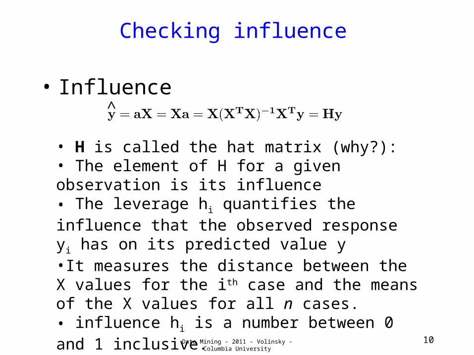
Checking influence
• Influence
• H is called the hat matrix (why?):• The element of H for a given observation is its influence• The leverage hi quantifies the influence that the observed response yi has on its predicted value y•It measures the distance between the X values for the ith case and the means of the X values for all n cases.• influence hi is a number between 0 and 1 inclusive.
^
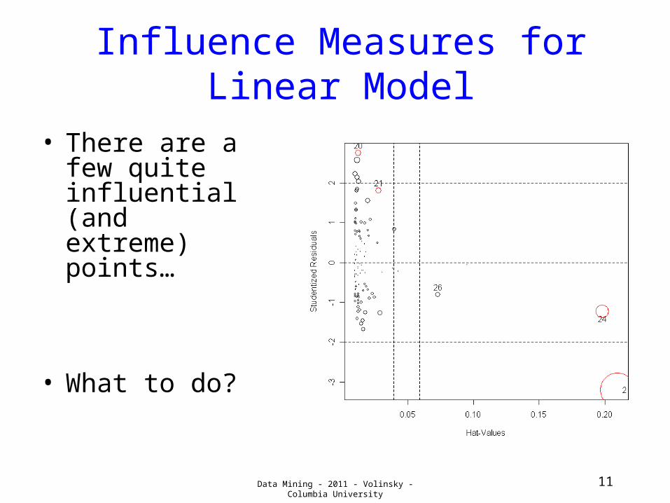
Influence Measures for Linear Model
• There are a few quite influential (and extreme) points…
• What to do?
11Data Mining - 2011 - Volinsky - Columbia University
Data Mining - 2011 - Volinsky - Columbia University 12
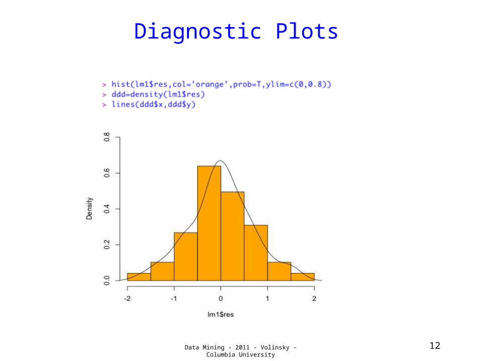
Diagnostic Plots

Data Mining - 2011 - Volinsky - Columbia University 13

Data Mining - 2011 - Volinsky - Columbia University 14
Model selection: finding the best k variables
• If noisy variables are included in the model, it can effect the overall performance.
• Best to remove an predictors which have no effect, lest random patterns look significant.
• Searching all possible models– How many are there?– Heuristic search is used to search over model space:
• Forward or backward stepwise search• Leaps and bound techniques do exhaustive search
– In-sample: penalize for complexity (AIC, BIC, Mallow’s Cp)
– Out-of-sample: use cross validation

Data Mining - 2011 - Volinsky - Columbia University 15
R ‘step’: uses AIC
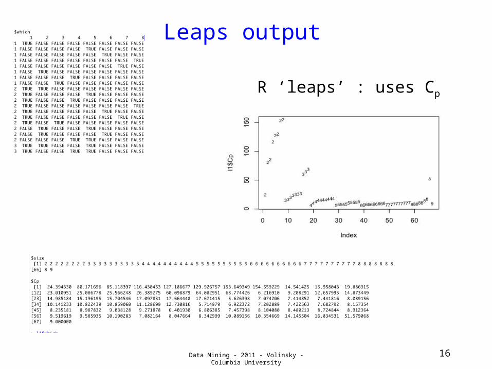
Leaps output
Data Mining - 2011 - Volinsky - Columbia University 16
R ‘leaps’ : uses Cp

Data Mining - 2011 - Volinsky - Columbia University 17
Generalizing Linear Regression

Data Mining - 2011 - Volinsky - Columbia University 18
Complexity versus Goodness of Fit
x
yTraining data

Data Mining - 2011 - Volinsky - Columbia University 19
Complexity versus Goodness of Fit
x
y
x
yToo simple?Training data
Data Mining - 2011 - Volinsky - Columbia University 20
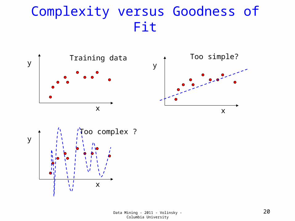
Complexity versus Goodness of Fit
x
y
x
y
x
y
Too simple?
Too complex ?
Training data
Data Mining - 2011 - Volinsky - Columbia University 21
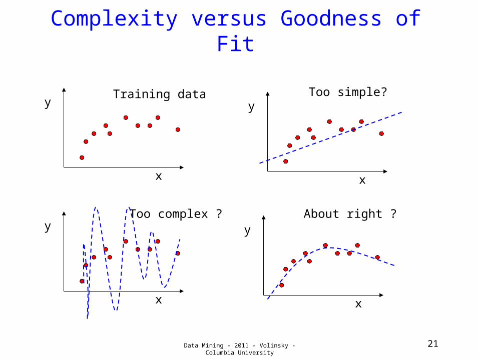
Complexity versus Goodness of Fit
x
y
x
y
x
y
x
y
Too simple?
Too complex ? About right ?
Training data

Data Mining - 2011 - Volinsky - Columbia University 22
Complexity and Generalization
Strain()
Stest()
Complexity = degreesof freedom in the model(e.g., number of variables)
Score Functione.g., squarederror
Optimal modelcomplexity

Data Mining - 2011 - Volinsky - Columbia University 23
Non-linear models, linear in parameters
• We can add additional polynomial terms in our equations,
• non-linear functional form, but linear in the parameters (so still referred to as “linear regression”)– We can just treat the xi xj terms as additional fixed inputs– In fact we can add in any non-linear input functions!, e.g.
Comments:- Number of parameters can explode => greater chance of
overfitting– Adding complexity: must use penalties!
Data Mining - 2011 - Volinsky - Columbia University
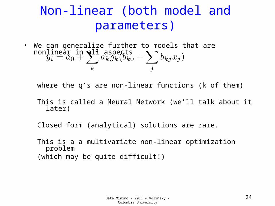
Non-linear (both model and parameters)
• We can generalize further to models that are nonlinear in all aspects
where the g’s are non-linear functions (k of them)
This is called a Neural Network (we’ll talk about it later)
Closed form (analytical) solutions are rare.
This is a a multivariate non-linear optimization problem(which may be quite difficult!)
24
Data Mining - 2011 - Volinsky - Columbia University 25
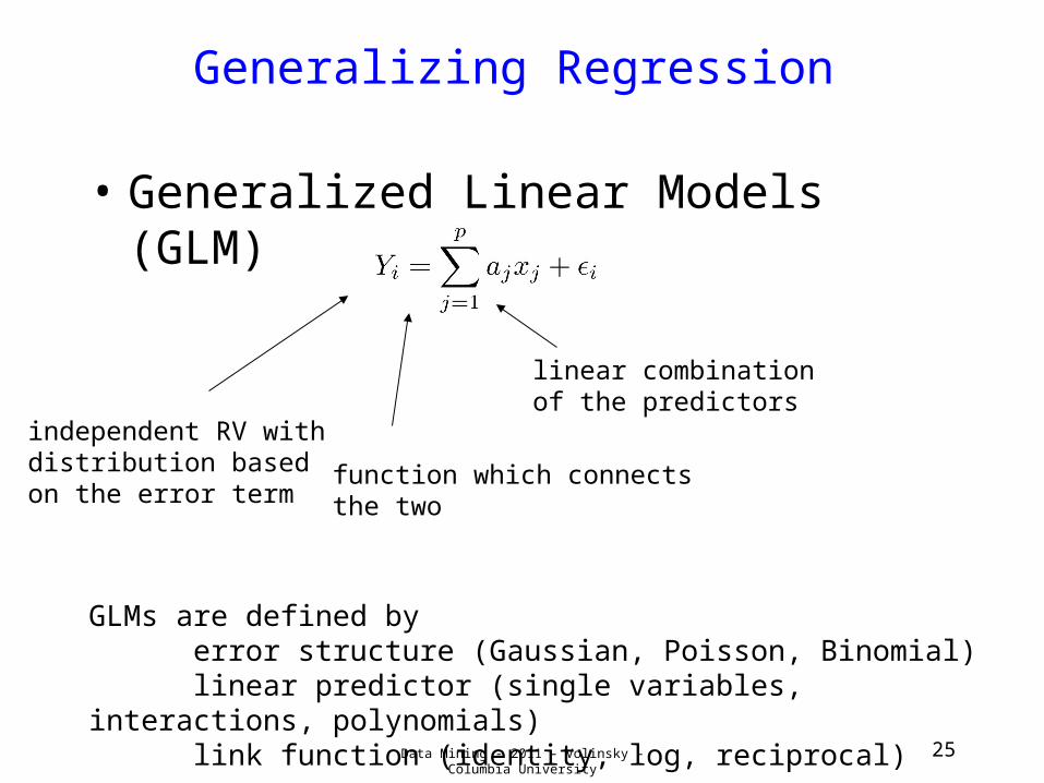
Generalizing Regression
• Generalized Linear Models (GLM)
independent RV with distribution based on the error term
linear combination of the predictors
function which connects the two
GLMs are defined byerror structure (Gaussian, Poisson, Binomial)linear predictor (single variables, interactions,
polynomials)link function (identity, log, reciprocal)

Data Mining - 2011 - Volinsky - Columbia University 26
Logistic Regression
• Logistic regression is the most common GLM. • response in this case is binary (0,1). (Y follows a
bernoulli or Binomial distribution)• we model the probability of a 1 (p) occurring. • for mathematical convenience, we model the odds:
– p/(1-p) – log odds are even better - logit function– scales on the real line, rather than [0,1]
• Deviance: -2 x (difference in log-likelihood from saturated model)

Logistic Regression
• Interpretation of coefficients changes!
Data Mining - 2011 - Volinsky - Columbia University 27
Data Mining - 2011 - Volinsky - Columbia University 28
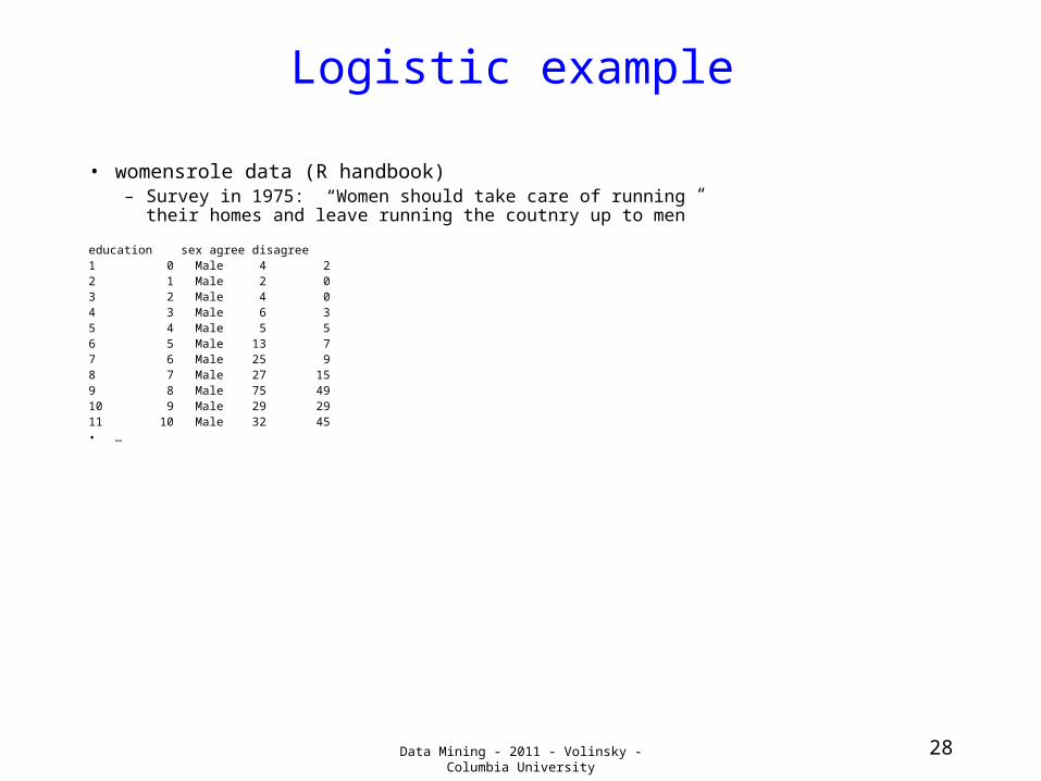
Logistic example
• womensrole data (R handbook)– Survey in 1975: “Women should take care of running their
homes and leave running the coutnry up to men”
education sex agree disagree1 0 Male 4 22 1 Male 2 03 2 Male 4 04 3 Male 6 35 4 Male 5 56 5 Male 13 77 6 Male 25 98 7 Male 27 159 8 Male 75 4910 9 Male 29 2911 10 Male 32 45• …

Data Mining - 2011 - Volinsky - Columbia University 29
Womensrole Logistic fit
Data Mining - 2011 - Volinsky - Columbia University 30
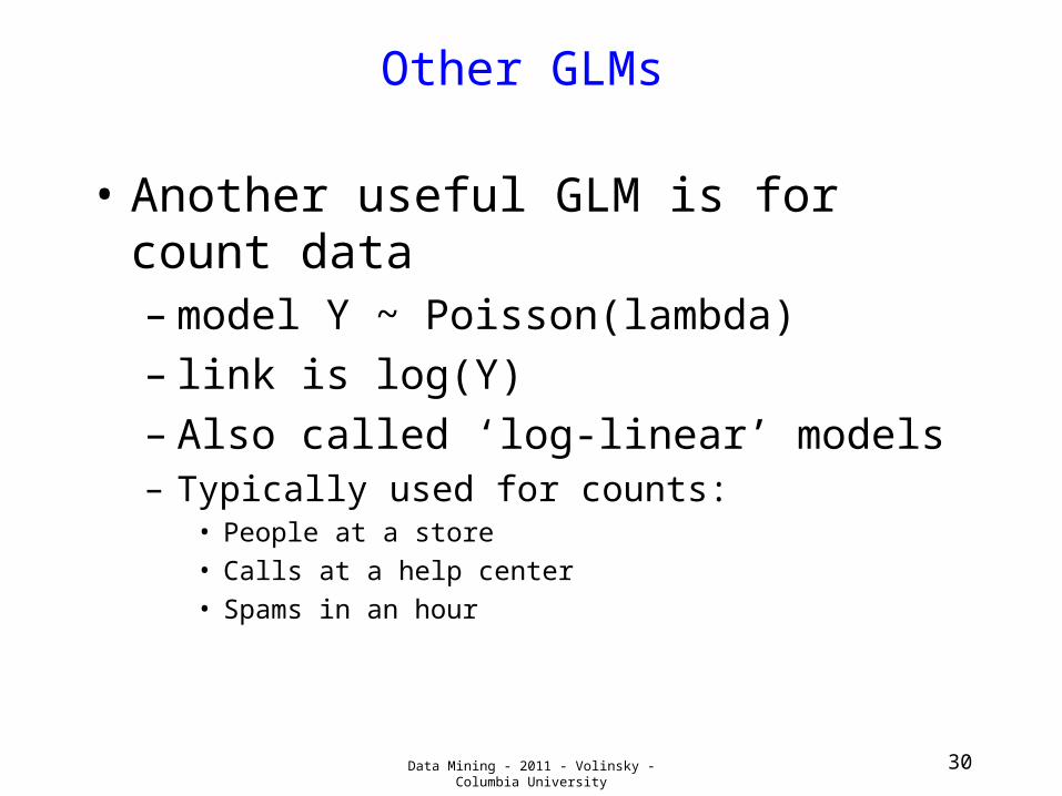
Other GLMs
• Another useful GLM is for count data– model Y ~ Poisson(lambda)– link is log(Y)– Also called ‘log-linear’ models– Typically used for counts:
• People at a store• Calls at a help center• Spams in an hour
Data Mining - 2011 - Volinsky - Columbia University 31
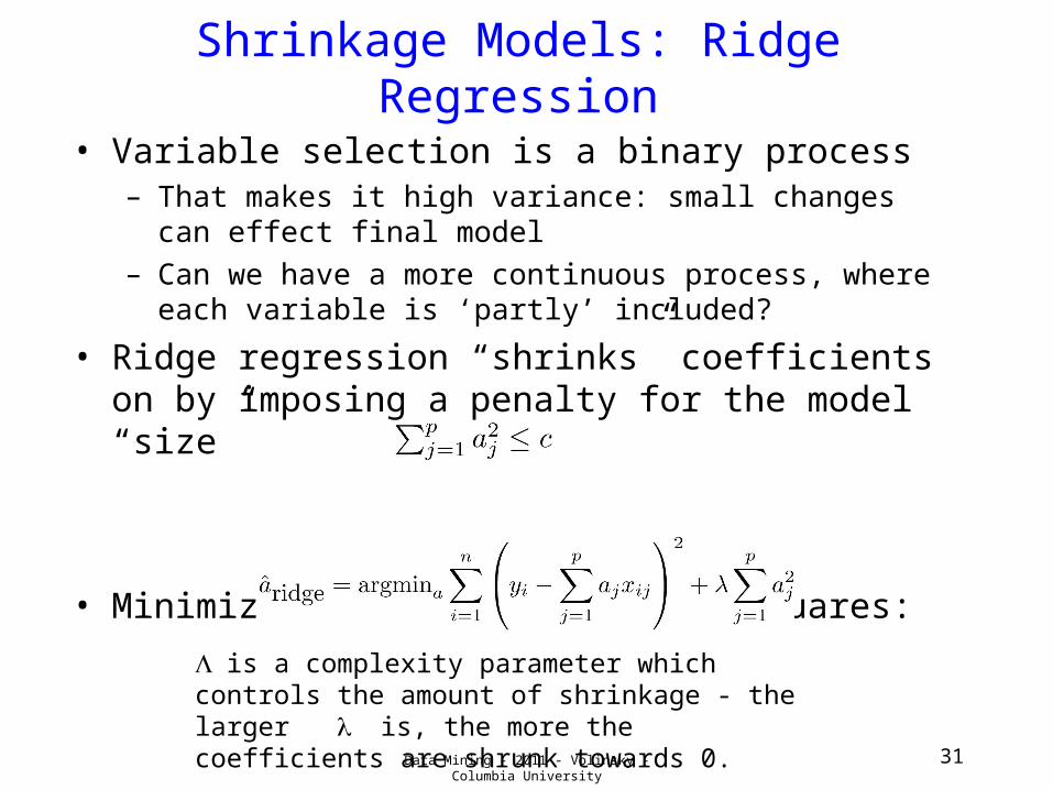
Shrinkage Models: Ridge Regression
• Variable selection is a binary process– That makes it high variance: small changes can
effect final model– Can we have a more continuous process, where
each variable is ‘partly’ included?
• Ridge regression “shrinks” coefficients on by imposing a penalty for the model “size”
• Minimize the penalized sum of squares:
is a complexity parameter which controls the amount of shrinkage - the larger is, the more the coefficients are shrunk towards 0.

Data Mining - 2011 - Volinsky - Columbia University 32
Ridge Regression
• Model is imposing a penalty on the coefficient size
• Since a’s depend on the units, care must be taken to standardize inputs.
• Also, you can show that the ridge estimates are a linear function of y:
• this adds a positive constant to the diagonal and allows inverision even if the matrix is not full rank– So, can be used in cases where p > n!
• In general: increasing bias, decreasing variance– Often decreases MSE

Data Mining - 2011 - Volinsky - Columbia University 33
Ridge coefficients
df() is a one-to-one monotone function of such that df() ranges from 0 to p.
= 0; s=p : least squares solution; p degrees of freedom
= inf; s=0; heaviest shrinkage; all parameter estimates = 0; zero degrees of freedom
Look at plot as a function of degrees of freedom
df()

Data Mining - 2011 - Volinsky - Columbia University 34
Lasso
• Very similar to ridge with one important difference:
• L2 penalty replaced by L1
• has an interesting effect on the profile plot:– if lambda is large then estimates go to zero– continuous variable selection– s=1 is least squares answer– s=0 all estimates are 0– s=0.5 was the value chosen by cross validation

lasso coefficients
Note how parameters shrink to zero!
This is the appeal of lasso (in addition to good performance)
Data Mining - 2011 - Volinsky - Columbia University
35s = df() / p
Principal Components Regression
• Create PC from the original data vectors and use them in any of the above regression schemes
• Removes the ‘less important’ parts of the data space, while creating a reduced data set
• Since each PC is a linear combination of the original variables, we can express the solution in terms of the initial coefficients.
Data Mining - 2011 - Volinsky - Columbia University 36
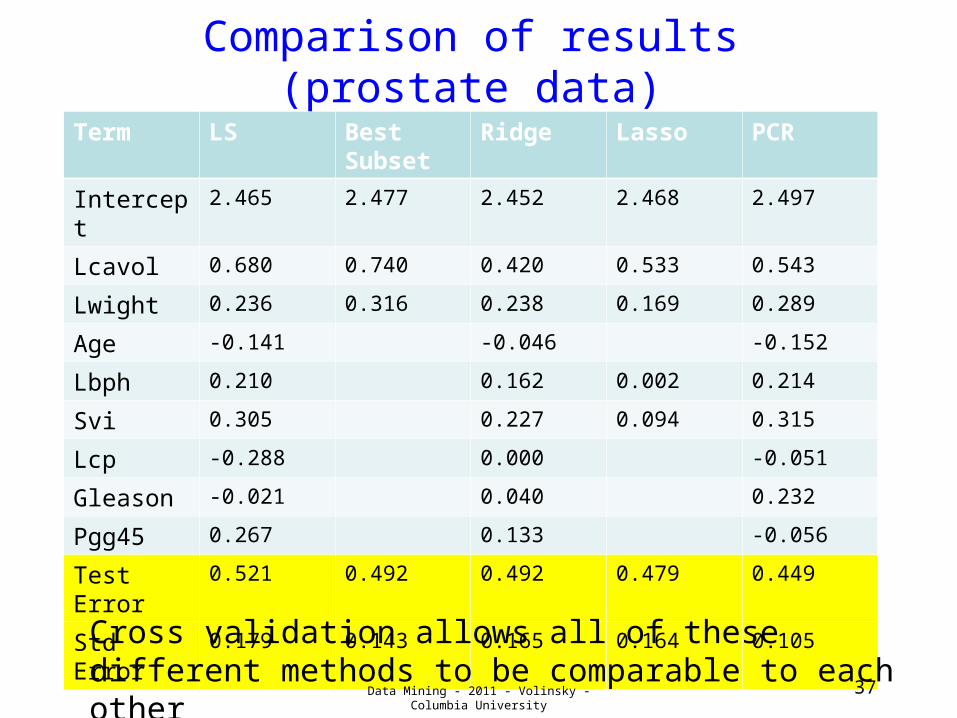
Comparison of results (prostate data)
Term LS Best Subset
Ridge Lasso PCR
Intercept 2.465 2.477 2.452 2.468 2.497
Lcavol 0.680 0.740 0.420 0.533 0.543
Lwight 0.236 0.316 0.238 0.169 0.289
Age -0.141 -0.046 -0.152
Lbph 0.210 0.162 0.002 0.214
Svi 0.305 0.227 0.094 0.315
Lcp -0.288 0.000 -0.051
Gleason -0.021 0.040 0.232
Pgg45 0.267 0.133 -0.056
Test Error
0.521 0.492 0.492 0.479 0.449
Std Error 0.179 0.143 0.165 0.164 0.105
Data Mining - 2011 - Volinsky - Columbia University 37
Cross validation allows all of these different methods to be comparable to each other
Nonparametric Modeling
• A nonparametric model does not assume any parameters to be estimated (thus the name nonparametric)– Its general form is Y = f(X) + ε– Typically, we only assume that f() is some
smooth, continuous function– Also, we typically assume independent and
identically distributed errors, ε~N(0,σ^2), but that’s not necessary.
– 1-D nonparametric regression = density estimation
38Data Mining - 2011 - Volinsky - Columbia University

Advantages & Disadvantages
• Advantage– More flexibility leads to better data-
fit, often also to better predictive capabilities
– Smoothness can also lead to entirely new concepts, such as dynamics (via derivatives) and thus to flexible differential equation models, etc
• Disadvantage– Much more complexity, hard to
explain
39Data Mining - 2011 - Volinsky - Columbia University

Fitting Nonparametric models
• How do we estimate the function f()?
– Restrictions on f: smoothness, continuity, existence of the first and second derivatives
– options for estimating f include scatterplot smoothers, regression splines, smoothing splines, B-splines, thin-plate splines, wavelets, and many, many more…
– one particularly popular option, the smoothing spline
40Data Mining - 2011 - Volinsky - Columbia University

Splines
• Splines are piecewise polynomials smoothly connected together. The joining points of the polynomial pieces are called knots.
• Smoothing splines are splines that are penalized against too much local variability (and thus appear smoother) – Must be differentiable at the knots– linear spline: 0-times differentiable– cubic spline: twice differentiable
41Data Mining - 2011 - Volinsky - Columbia University

Piecewise Polynomial cont.
• Piecewise constant and piecewise linear
“Knots”
42Data Mining - 2011 - Volinsky - Columbia University

Spline cont. (Linear Spline)
43Data Mining - 2011 - Volinsky - Columbia University

Spline cont. (Cubic Spline)
Cubic spline
44Data Mining - 2011 - Volinsky - Columbia University

Definition of Smoothing Splines
• Smoothing Splines arise as the solution to the following simple regression problem– Find a piecewise polynomial f(x) with smooth
breakpoints
– f(x) minimizes the penalized sum-of-squares
€
RSS( f ,λ ) = {y i − f (x)}2
i=1
n
∑ + λ { ′ ′ f (t)}2∫ dt
fit curvature
45Data Mining - 2011 - Volinsky - Columbia University
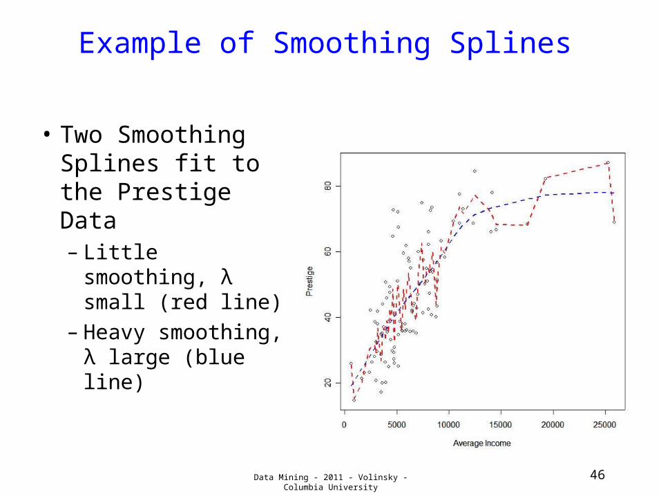
Example of Smoothing Splines
• Two Smoothing Splines fit to the Prestige Data– Little smoothing,
λ small (red line)– Heavy
smoothing, λ large (blue line)
46Data Mining - 2011 - Volinsky - Columbia University
The smoothing parameter
• The magnitude of λ affects the quality of the smoother; many ad-hoc approaches to find a “good” smoothing parameter– Visual trial and error– Minimize mean-squared error of the
fit– Cross-validation, optimization on
hold-out sample, etc
47Data Mining - 2011 - Volinsky - Columbia University
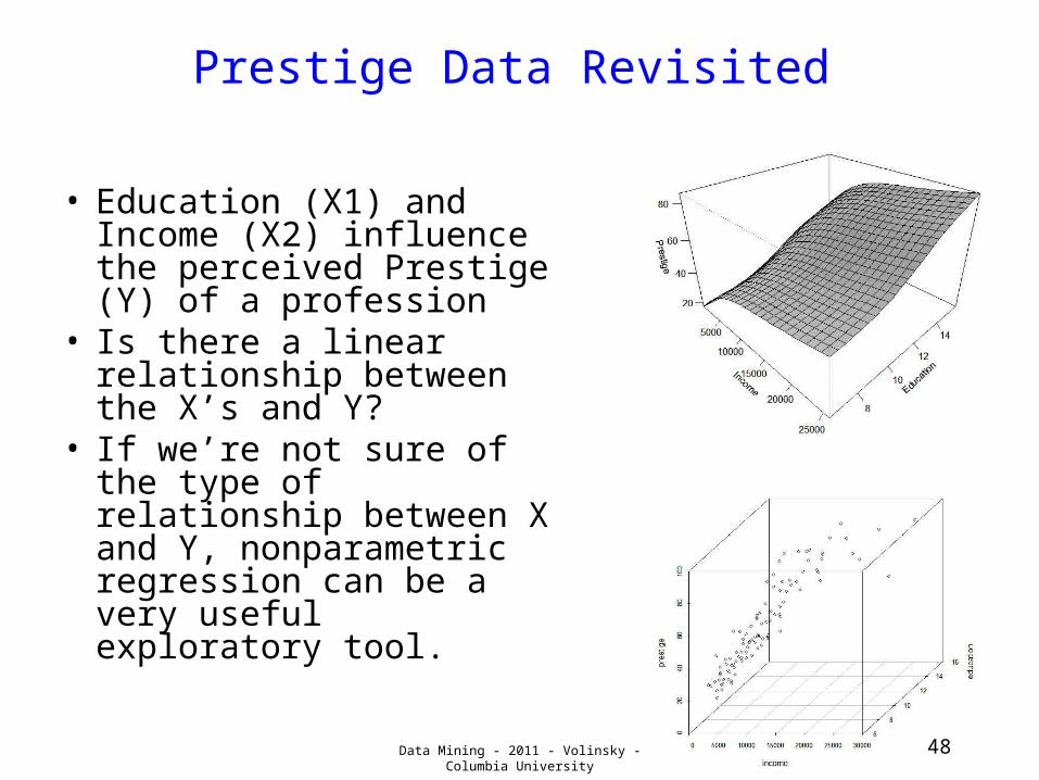
Prestige Data Revisited
• Education (X1) and Income (X2) influence the perceived Prestige (Y) of a profession
• Is there a linear relationship between the X’s and Y?
• If we’re not sure of the type of relationship between X and Y, nonparametric regression can be a very useful exploratory tool.
48Data Mining - 2011 - Volinsky - Columbia University
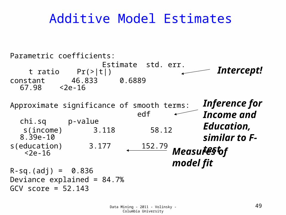
Additive Model Estimates
Parametric coefficients: Estimate std. err. t ratio
Pr(>|t|)constant 46.833 0.6889 67.98
<2e-16
Approximate significance of smooth terms: edf chi.sq p-value s(income) 3.118 58.12 8.39e-10s(education) 3.177 152.79 <2e-
16
R-sq.(adj) = 0.836 Deviance explained = 84.7%GCV score = 52.143
Intercept!
Inference for Income and Education, similar to F-testMeasures of
model fit
49Data Mining - 2011 - Volinsky - Columbia University

Compare to Classical Regression
Parametric coefficients: Estimate std. err. t ratio
Pr(>|t|)(Intercept) -6.8478 3.219 -2.127
0.0359 income 0.0013612 0.000224 6.071 2.36e-
08 education 4.1374 0.3489 11.86 <2e-
16
R-sq.(adj) = 0.794 Deviance explained = 79.8%GCV score = 62.847
Better model fit for the nonparametric model!!
50Data Mining - 2011 - Volinsky - Columbia University

Function Estimates from Additive Regression Model
• What is the nature of the relationship of the individual predictor variables and prestige?
51Data Mining - 2011 - Volinsky - Columbia University